© The Authors 2026

1 Introduction

The Planck space mission, launched by ESA in 2009, has provided the astronomical community with an unprecedented view of the microwave sky emission in nine frequency bands ranging from 30 GHz to 857 GHz. Seven of the Planck mission frequency channels, between 30 GHz and 353 GHz, were polarization-sensitive and have mapped a mixture of polarized emission from the cosmic microwave background (CMB) and from the interstellar medium (ISM) of our own Galaxy, the Milky Way (Planck Collaboration 2020a). The Planck space mission data products have been made available to the scientific community in the Planck Legacy Archive at ESA¹.

The next generation of ground-based CMB observations is now focusing on precisely measuring CMB polarization, which is expected to carry the tiny signature of primordial gravitational waves generated during a phase of cosmic inflation (Kamionkowski & Kovetz 2016). However, detecting polarized CMB is difficult because it is subdominant at all frequencies compared to polarized Galactic emission. The main Galactic contaminant above ~70 GHz is polarized dust emission from the Galactic ISM, which arises from the preferential alignment of elongated dust grains perpendicular to the Galactic magnetic field. Below ~70 GHz, polarized synchrotron emission from relativistic electrons dominates.

Traditionally, these different signals have been separated by exploiting their different emission laws as a function of frequency (Delabrouille & Cardoso 2009). This requires observations in frequency bands at least in the 30 to 300 GHz frequency range, and preferably more. However, observations above 220 GHz are challenging from ground-based observatories, because of strong fluctuating atmospheric emission and absorption. This motivates the use of external templates of polarized dust emission to help with the analysis of future ground-based observations. Such maps have been made available as part of the Planck mission data releases (Planck Collaboration 2020c), but the published maps are either strongly filtered or dominated by noise in the regions of the sky with the lowest polarized dust emission, which are of the greatest interest for current and future CMB observations. This paper aims to demonstrate how higher-quality polarized dust maps can be constructed from Planck data.

To do so, a promising new direction is to rely on recently developed scattering transforms (STs) (Bruna & Mallat 2013). These provide a mathematically grounded set of low-variance summary statistics that efficiently capture the non-Gaussian features of complex physical fields. Inspired by convolutional neural networks but defined analytically, they characterize interactions between oriented spatial scales through cascades of wavelet convolutions and nonlinear operations, as well as covariance estimates, producing compact and interpretable descriptors that go beyond traditional power-spectrum analyses. Because they require no training and can be estimated from limited data, STs have proven highly effective across a range of astrophysical and cosmological applications (Allys et al. 2019; Regaldo-Saint Blancard et al. 2020; Cheng & Ménard 2021; Valogiannis & Dvorkin 2022; Lei & Clark 2023; Hothi et al. 2024).

In addition to classification and parameter inference, ST have also been used to construct generative models of physical fields, in a maximum entropy framework. These quantitatively realistic models, constrained from the ST statistics themselves, can even be constructed from a single realization of the process under study (Allys et al. 2020; Cheng et al. 2024; Mousset et al. 2024). They enable the synthesis of new, statistically consistent realizations that preserve the multiscale, non-Gaussian texture of various data types without any prior knowledge of the underlying physics or the need for extensive training sets. In Jeffrey et al. (2022), it was shown in particular that a ST-based generative model constructed from a single polarized dust patch could be used to train a neural network capable of separating CMB B modes from Galactic dust emission, underscoring the potential of this framework for Galactic emission modeling.

The ability to sample new realizations, which is done using a pixel-based gradient descent under ST constraints (Bruna & Mallat 2019), has been extended to component separation tasks. In Regaldo-Saint Blancard et al. (2021), this approach was introduced to separate the Galactic dust emission from instrumental noise in Planck 353 GHz polarization maps. It was then extended in Delouis et al. (2022) to full-sky data, dust polarization maps that remain statistically reliable even at scales where the dust power is significantly below the noise level. More recently, Auclair et al. (2024) applied such a ST-based component separation to Herschel observations, showing that two distinct non-Gaussian processes – Galactic dust emission and the cosmic infrared background – could be statistically separated from observational data alone, within a single-frequency framework. These approaches were also complemented by machine learning when sufficient data was available. This allowed an unsupervised ST modeling of components from unlabeled mixtures to be performed using variational auto-encoders (VAEs), for both seismic data (Siahkoohi et al. 2023b,a) and radio observations of the different phases of the ISM (Lei et al. 2025). These results demonstrate the great promise of such approaches.

In this paper, we extend previous ST-based component separation approaches to construct maps of polarized dust emission at 353 GHz with significantly improved angular resolution and reduced noise contamination compared to current state-of-the-art methods. The key novelties of our approach include the use of the most recent state-of-the-art ST statistics, the incorporation of information from 857 GHz intensity maps to inform and constrain the separation of Q and U polarized components, making use of local polarization reference axes, and the extensive use of complementary constraints.

The paper is structured as follows. Section 2 presents the observational data used in this work, as well as their preliminary processing. Section 3 presents the mathematical formulation of the problem and the optimization scheme used to recover the component-separated maps. Section 4 presents the results of our component separation algorithm on a sky patch and evaluates its performance using an independent validation patch. Finally, Section 5 presents our conclusions.

2 Data

2.1 Set of maps used and preprocessing

This paper focuses on producing a de-noised dust polarization map in the 353 GHz Planck frequency band. Polarized dust emission maps have been previously published by the Planck collaboration (Planck Collaboration 2020c). Maps obtained with the Commander (Eriksen et al. 2006), GNILC (Remazeilles et al. 2011), and SMICA (Delabrouille et al. 2003; Cardoso et al. 2008) methods have been made available on the Planck Legacy Archive. However, these maps, obtained in analyses for which the CMB was the primary objective, are either at degraded angular resolution (GNILC) or still significantly contaminated by residual noise (SMICA and Commander).

In this paper, we used the Planck NPIPE PR4 maps (Planck Collaboration 2020b), which offer the highest signal-to-noise ratio (S/N) for dust polarization among available Planck maps. These maps include a small CMB polarization contribution, which we reduced by subtracting a multivariate Wiener-filtered estimate derived from the Planck I, E, and B maps². The maps were convolved with a Gaussian beam with an effective full width at half maximum (FWHM) of 10 arcmin, assuming an FWHM of 4.76 arcmin for the original PR4 maps, and converted to megajanskys per steradian. The resulting Q and U maps are denoted d_Q and d_U.

To perform the component separation, we relied on a model of the signals other than dust at this frequency, the instrumental noise and the CMB residual, the sum of which we call the contamination. To do so, we constructed an ensemble of one hundred 353 GHz Q and U contamination maps, as described in Appendix B. These maps, which are also convolved to a resolution of 10 arcmin, are called {C_Q,I, c_U,i}, for i between 1 and 100.

In this paper, we also relied on the total intensity emission of dust, which is a good indicator of the location and shape of the dust structures that contribute to 353 GHz dust polarization maps. The Planck-HFI 353 GHz to 857 GHz maps are good tracers of this emission. Among those, we selected the Planck NPIPE PR4 857 GHz map, which has the best S/N and is the least contaminated by cosmic infrared background (CIB) and CMB intensity fluctuations relatively to dust emission (see Fig. 1). Minimal preprocessing was performed on this map to detect and subtract emission from external galaxies and from the dense regions in the ISM in the Milky Way. We also readjusted the zero-level of the map by fitting a cosecant law to map emission at Galactic latitudes of |b| > 10°. This last map, which is also at 10 arcmin, is called d_I.

We compare our results to representative state-of-the-art polarized foreground products from the Planck PR3 release: GNILC (Remazeilles et al. 2011), SMICA (Delabrouille et al. 2003; Cardoso et al. 2008), and Commander (Eriksen et al. 2006). GNILC is a multifrequency, scale-dependent component separation method operating in needlet space, using local covariance estimates to isolate the foreground subspace while suppressing noise and CMB contamination (Remazeilles et al. 2011). SMICA performs spectral matching of empirical covariance matrices across frequencies and scales, while Commander performs a parametric Bayesian fit of the sky components in pixel space. Together, these products provide benchmarks for the quality of current Planck polarized foreground maps, each with different trade-offs in angular resolution, residual noise, and modeling assumptions.

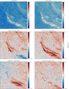Fig. 1 Signal maps of the patch of interest in our work centered at (l, b) = (315, 78.): Top left: I 353 GHz. Top right: I 857 GHz. Middle left: Q 353 GHz before polarization rotation. Middle right: Q 353 GHz after polarization rotation. Bottom left: U 353 GHz before polarization rotation. Bottom right: U 353 GHz after polarization rotation. In this paper, we only used the data from the right column.

2.2 Selection of square patches

In this paper, we only worked on square patches, whose extraction from HEALpix maps is discussed in Appendix A. We also discuss in this appendix the geometric convention used for the definition of Stokes parameters consistently for each map, which solves the coordinate dependence problem of the original Stokes Q and U maps, which creates artificial gradients along dust filaments as shown in Fig. 1. The size of the square patches is 384 × 384 pixels, and the linear scale of each pixel is ~3.4 arcmin.

We applied our component separation algorithm to two distinct regions. The first region is where we produced a dust map with an improved S/N and angular resolution. The second region, which already has a high S/N, is only used for validation. Specifically, we applied our component separation algorithm to this region after contaminating it such that the resulting map has a S/N similar to that of the first region we studied.

The first region corresponds to a patch centered at (l, b) = (315°, 78.3°), chosen because it is at a high Galactic latitude, and because it contains a significant dust filament located close to the center of the patch. Henceforth, we refer to this patch as the “north patch”. The I, Q, and U of this region can be seen in Fig. 1. The left column shows the I map at 353 GHz, and the original Q and U polarized map before the redefinition of the Stokes parameters. The right column corresponds to the fields that will be used below: d_I for the I field at 857 GHz, and d_Q, d_U, the rotated Q and U maps at 353 GHz.

Incidentally, one sees that this is a region where the original Q and U reference system rotates strongly across the patch. Indeed, by looking along the filament in the original Q and U maps, we see an anticorrelation along the filament in both cases, which underlines the dependence on the orientation of the local polarization basis. To solve that problem, we defined the coordinates properly by parallel transporting the reference axes from a chosen origin (the center of the patch, i.e., the center of a HEALPix superpixel at Nside = 4) to each pixel, thereby defining a common frame. This parallel transport provides the geometric foundation that makes the analysis of polarized dust foregrounds in terms of Q and U consistent and physically meaningful.

The validation patch is centered at (l, b) = (213.7°, −19.5°), where thermal dust emission clearly dominates over the nuisance. Henceforth, we refer to this as the “Orion patch”. To validate the method under conditions comparable to the northern patch, we artificially degraded the Orion patch before applying the algorithm: the original high-S/N Planck map was rescaled so that, after adding a nuisance realisation, its S/N matched that of the northern patch, creating a mock observation with a known ground truth. This rescaling was not required by the method itself; it was introduced only to make the validation representative of the lower-S/N regime in which the algorithm was ultimately applied. The initial rotated Q maps, as well as the surrogate d_Q map obtained after adding a nuisance realization, can be seen in Fig. 2.

3 Formalism and algorithm

3.1 Principle of the algorithm

For each polarization channel, the observed map for each Stokes parameter, a = Q, U, is taken to be the sum of the respective thermal-dust emission, s_a, and a contamination term, c_a, that includes both the CMB residuals and the instrumental noise: $$d_a=s_a+c_a.$$(1)

Our goal is to construct maps, ${\tilde{s}}_a$, that are statistically consistent with the data once the effect of the contamination is taken into account. To do so, we introduced an ensemble of constraints, estimated directly from the available data, that these maps have to fulfill. These constraints were written using an ensemble of auto- and cross-statistics, which we label Φ, and whose choice is discussed in the following.

Following recent developments (Regaldo-Saint Blancard et al. 2021; Delouis et al. 2022; Auclair et al. 2024), we proceeded by writing constraints in the statistics space that the prospective maps, ${\tilde{s}}_a$, must satisfy. The first of them are: $$\text{Φ}\left(d_a\right)\simeq {\langle \text{Φ}\left({\tilde{s}}_a+c_a\right)\rangle }_{c_a},$$(2) $${\langle \text{Φ}\left(c_a\right)\rangle }_{c_a}\simeq \text{Φ}\left(d_a-{\tilde{s}}_a\right),$$(3) $$\text{Φ}\left(d_Q,d_U\right)\simeq {\langle \text{Φ}\left(\begin{array}{cc}{\tilde{s}}_Q+c_Q,& {\tilde{s}}_U+c_U\end{array}\right)\rangle }_{c_Q}{}_{,c_U},$$(4)

where the average $\langle \cdot \rangle c_a$ is taken over the ensemble of contamination maps {c_Q,i, -, c_U,i} introduced in Sect. 2. Here, Eq. (2) imposes that ${\tilde{s}}_a+c_a$ is statistically compatible with the data, d_a, on average over {c_Q,i, c_U,i}. Similarly, Eq. (3) imposes that $d_a-{\tilde{c}}_a$ is statistically compatible with the contamination model. Finally, Eq. (4) extends Eq. (2) by imposing that the cross-statistics between ${\tilde{s}}_Q+c_Q$ and ${\tilde{s}}_U+c_U$ match those of the data.

While these constraints require statistical independence between the s_a maps and the contamination, an advantage is that they do not require any explicit knowledge of statistics involving only the s_a maps, as Φ(s_a) or cross-statistics between s_a and other maps. This framework thus allows us to efficiently use ancillary data, as long as they are independent, in the present case, of the contamination. In particular, we impose in this paper that ${\tilde{s}}_a$ must reproduce the observed cross-statistics with the 857 GHz intensity map d_I: $$\text{Φ}\left(d_a,d_I\right)\simeq {\langle \text{Φ}\left({\tilde{s}}_a+c_a,d_I\right)\rangle }_{c_a}.$$(5)

These constraints leverage the strong statistical dependency that is expected between these two signals, while not assuming a particular value for Φ(s_a, d_I). We note that such constraints could be used to leverage various types of ancillary data.

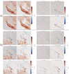Fig. 2 Top: results of our component separation algorithm for the Stokes Q component in the rotated polarization reference frame. The map labeled dQ is the CMB-subtracted Planck map, while ${\tilde{s}}_Q$ denotes the corresponding component-separated dust emission map. For comparison, the corresponding region of the GNILC map is shown. A random realization of the nuisance component, cQ,I, has been added to the ${\tilde{s}}_Q$ map to demonstrate statistical consistency with dQ. Similarly, the recovered nuisance $d_Q-{\tilde{s}}_Q$ is compared with a random realization of the noise. In addition, we plot dQ – GNILC in order to demonstrate the existence of dust residuals in the recovered nuisance map. Finally, the residual between ${\tilde{s}}_Q$ and the corresponding GNILC map is shown. Bottom: as above, but for the high-S/N region used for validation. Note that in this case the GNILC map is filtered to facilitate comparison with the results above. Finally, in the bottom row we compare the true signal, sQ, with the average $\langle {\tilde{s}}_Q\rangle$ of ensembles obtained by using different initial conditions, as well as the residual between the true signal, sQ, and the recovered, $\langle {\tilde{s}}_Q\rangle$, and with the recovered GNILC.

3.2 Choice of statistics and gradient descent optimization

Gradient descent objective functions. The recovery of ${\tilde{s}}_a$ was carried out through a gradient–descent optimization in pixel space, whose objective function takes the form of a sum of seven loss functions, one for each of the constraints of Eqs. (2)–(5) and each value of a. For example, the loss associated with the constraint given in Eq. (2) for the Stokes Q channel yields $${ℒ}_1\left(u_Q\right)=\frac{1}{M}{\displaystyle \sum _{i=1}^M{\left|\text{Φ}\left(u_Q+c_{Q,i}\right)-\text{Φ}\left(d_Q\right)\right|}^2}.$$(6)

These losses involve u_a (i.e., u_Q and u_U), the “running maps” on which optimization is performed, the final values of which correspond to ${\tilde{s}}_a$ (i.e., ${\tilde{s}}_Q$ and ${\tilde{s}}_U$) after convergence of the gradient descent. The explicit form of the other individual loss functions is given in Eqs. (C.3)–(C.6) in Appendix C, and their purpose is schematically summarized in Table 1. The total objective function to be minimized is formed as the sum of all seven individual losses.

In this paper, we performed this gradient descent starting from the data, d_a, which lead to a single point-estimate, ${\tilde{s}}_a$, for each Stokes parameter after convergence. These maps, which verify constraints given Eqs. (2)–(5), are expected to accurately reproduce the statistical properties of s_a, at least at scales where the relative amplitude of the contamination is not too high. However, it should be noted that they do not necessarily reproduce the deterministic structures in s_a at scales where the contamination is non-negligible (see Regaldo-Saint Blancard et al. (2021); Delouis et al. (2022) for a discussion on this point).

We also produced a set of two $\langle {\tilde{s}}_a\rangle$ maps that are close to Sa from a deterministic point of view (i.e., whose mean square error in pixel space is lower), which allows for a better comparison to GNILC. We did so by sampling additional maps close to the ${\tilde{s}}_a$ map, which verify constraints Eqs. (2)–(5), but whose structures differ at scales where the recovery is not deterministic anymore. These maps were obtained with the same algorithm as is described above, but using ${\tilde{s}}_a+c_{a,i}$ as initial conditions, where c_a,i are drawn from the nuisance ensemble. An ensemble average was then performed on these maps to produce $\langle {\tilde{s}}_a\rangle$, which is expected to be closer deterministically to the true map, as only the structures that are consistently reproduced along the different samples remain after averaging. It should be noted, however, that these maps no longer verify the constraints given Eqs. (2)–(5), since the structures at small scales are for instance smoothed.

While it seems clear from the results discussed below that the ${\tilde{s}}_a$ maps and $\langle {\tilde{s}}_a\rangle$ maps better reproduce the statistical and deterministic properties of s, respectively, a drawback of our approach is that we are currently unable to provide consistent uncertainty estimates for these maps. We note that the ensemble of maps obtained by using different initial conditions is not intended to provide a proper uncertainty quantification, since there is no reason to expect these samples to sufficiently explore the landscape in the neighborhood of the maximum-likelihood estimate. In this paper, the role of this variability is instead to average out as best as possible the statistical fluctuations present at the smallest scales. However, the task of uncertainty quantification has been tackled in parallel for a similar framework, but with a mono-frequency and single-constraint problem (Pierre et al. 2026). Extending such an approach to the present multi-constraint setting is left to future work.

Choice of statistics. Although, in principle, any choice of summary statistics, φ, is possible, in practice they are selected to guarantee the stability of the pixel–space gradient descent, as well as to efficiently characterize the non-Gaussian features of the polarized foreground emission. As is demonstrated in Cheng et al. (2024) and Mousset et al. (2024), scattering covariance statistics have shown great promise in both regards. These form a family of ST statistics that are computed by calculating the covariances between the scattering coefficients computed at different oriented scales. For their mathematical definition and the explicit definition of φ, see Appendix C.

Following these references, we adopted a normalization, estimated on the target side of the losses, that balances the relative contributions of large and small scales. Indeed, complex multiscale physical processes typically exhibit a falling power-law behavior in the power spectrum, leading to high-frequency modes being subdominant in the loss if the coefficients are left unnormalized. To compensate for this, we normalized φ so that all scales contribute with comparable weight. The specific normalization is shown in Appendix C. We note that for a single loss term, as was the case in Regaldo-Saint Blancard et al. (2021), the algorithm was found to perform better with a refined normalization putting more weight to the small scales. However, when multiple losses are combined simultaneously, it seems that the uniform normalization proposed in this paper gives very good results while being simple and stable.

3.3 Practical implementation

In order to work with 384 × 384 pixels maps, an ensemble of J_max = 7 absolute dyadic scales and L = 4 orientations was used for all scattering–covariance computations (see Appendix C for definitions). Here, J_max denotes the number of dyadic scales used in the scattering analysis, with the coarsest scale considered being $2^{J_{\text{max}}}$. This choice fixes the number of coefficients entering each loss term: for single–field statistics, Φ(x), the total number of coefficients is 5 011, while for cross–field statistics, Φ(x₁, x₂), it is 17 960. These values determine the dimensionality of the constraints appearing in each of the seven losses, and thus in the objective function.

The optimization was performed in PyTorch using a limited-memory Broyden–Fletcher–Goldfarb–Shanno (L-BFGS) optimizer (Nocedal 1980). At each iteration, every loss term was evaluated over a random batch of ten nuisance realizations, yielding a stochastic approximation of the expectation over contamination while maintaining the efficiency of a quasi-Newton update. The seven loss terms were combined with equal weight, i.e., no additional reweighting between constraints was introduced beyond the normalization of the scattering coefficients discussed above. Optimization was stopped after 35 steps for each iteration. The values of the batch size, number of optimization steps, and number of samples used to build the ensemble maps were chosen empirically as a compromise between convergence stability and computational cost. For 384 × 384 maps, the gradient–descent procedure converges in approximately 20 minutes on an NVIDIA A100 80 GB GPU. In order to compute the ensemble maps, ${\overline{s}}_a$, we used 33 samples for both the northern patch and Orion patch.

4 Results

4.1 North patch

In Fig. 2, we present the results of our component-separation method applied to the north patch. We clearly see in it that the recovered map, ${\tilde{s}}_Q$, reconstructs small-scale non-Gaussian structures beyond the noise level. In contrast, the GNILC map of this region appears to smooth out fine-scale fluctuations, illustrating the stronger filtering applied by that method. By visual inspection, one also observes that the composite maps ${\tilde{s}}_Q+c_{Q,i}$ closely resemble d_Q, and that the residuals $d_Q-{\tilde{s}}_Q$ similarly resemble the nuisance realizations, c_Q, indicating good statistical proximity in both comparisons. For each of these comparisons, we emphasize that while visual agreement is not a sufficient condition, achieving it is a very good indicator of similar non-Gaussian structures.

The power spectra corresponding to the previous comparisons are shown in Fig. 3. These spectra were computed on apodized maps and binned to reduce statistical variance at high-k modes. At the spectral level, we observe that the power spectrum of $\langle {\tilde{s}}_Q+c_Q\rangle$ agrees with that of d_Q within the one sigma level estimated from the nuisance variability. Further, the power spectrum of $d_Q-{\tilde{s}}_Q$ also agrees with that of the nuisance maps within one sigma of the nuisance. The power spectrum of ${\tilde{s}}_Q$ is also compared with that of the polarized dust emission inferred from the cross-correlation of two half-ring observations of the same sky patch. Within the apparent variance of the half-ring cross-spectrum, the recovered Q-component power spectrum shows good agreement. The power spectrum of the corresponding GNILC map is shown for reference. In Fig. 4, we show the original and decontaminated maps for the Q and U polarization channels, as well as for the polarized intensity, in the northern patch.

In Fig. D.1, we compare the reconstructed dust polarization map obtained from our method with three state-of-the-art simulated dust models from PySM 3 (Thorne et al. (2017); Zonca et al. (2021); The Pan Experiment Group (2025)) corresponding to increasing levels of physical complexity. Models d9, d10, and d12 represent, respectively, a single–modified black-body model with fixed parameters, a spatially varying modified blackbody model, and a six independent layers dust model that accounts for multiple dust populations along the line of sight (Martínez-Solaeche et al. 2018). From this comparison, it appears that our method is able to recover non-Gaussian structures that are more compatible with the data than the previous models.

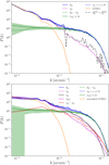Fig. 3 Top: power spectra of the maps shown in Fig. 2a. The solid blue line shows the initial Planck map dQ, while the dashed blue line (with 1σ margin) corresponds to the recovered map after adding the nuisance. The dashed purple line correspond to the recovered dust signal, ${\tilde{s}}_Q$. For comparison, the power spectrum of the true polarized dust emission is approximated by taking the cross-spectrum of the two half-ring maps (dash-dotted black line). The solid purple line corresponds to the average recovered signal $\langle {\tilde{s}}_Q\rangle$ (see Sect. 3.2). Finally, the solid and dashed green lines correspond to the nuisance (with 1σ margin) and recovered nuisance maps. For comparison, the power spectrum of the filtered GNILC map is also shown in orange. Bottom: as above, but for the maps of Fig. 2b. In this case, the power spectrum of the true polarized dust emission (solid black line) is known.

4.2 Validation on the Orion patch

To validate our method, we applied the algorithm to the rescaled Orion patch (see Sect. 2.2). Figure 2 shows the resulting output maps, similarly than for the north patch. The map ${\tilde{s}}_Q+c_{Q,i}$ seems to agree with the mock observation, d_Q, suggesting statistical consistency between the reconstructed and observed map. Similarly, the residual map, $d_Q-{\tilde{s}}_Q$, agrees well with the true nuisance, $c_Q^0$, confirming that the recovered nuisance component captures the expected statistical properties.

In addition, a visual comparison between the recovered map ${\tilde{s}}_Q$ and the ground truth s_Q indicates that the contamination has been effectively removed while preserving the non-Gaussian structure of the polarized dust emission, including at angular scales where the polarized 353 GHz signal is below the noise level. Comparing with the GNILC map also shows that many more structures appear to have been reconstructed. Note that, for this region, the GNILC map has been filtered to contain power at the same scales as the GNILC map for the north patch.

This type of recovery has previously been studied in Regaldo-Saint Blancard et al. (2021); Delouis et al. (2022), where it was demonstrated that a transition occurs between large (high-S/N) scales, which are recovered deterministically, and smaller (lower-S/N) scales, which have the correct statistical properties but do not match the true structure. This can be seen in the behavior of the power spectrum of $s_Q-{\tilde{s}}_Q$ in the bottom patch of Fig. 3, which is two orders of magnitude below the power spectrum s_Q at large scales, and crosses it only close to 0.7 arcmin⁻¹, where the algorithm breaks down. It should be noted that this recovery of the signal below the noise level is not related to any prior information on polarized emission, but rather to the strong constraints of recovering the same auto- and cross-statistics as those estimated from the data. Note that in this map, the GNILC map has been filtered so that it contains power in the same scales as in the GNILC map for the north patch.

Finally, the bottom row of Fig. 2 shows a comparison between the true s_q, $\langle {\tilde{s}}_Q\rangle$, and GNILC. Overall, $\langle {\tilde{s}}_Q\rangle$ provides a better small-scale deterministic reconstruction, as seen in the maps and their differences from the truth.

For this validation patch as for the north patch, Fig. 3 shows the power spectra of the different maps. We find that the power spectra of the recovered polarized dust emission, ${\tilde{s}}_Q$, and that of the true map, s_Q, are consistent across scales, demonstrating the success of our component-separation even at scales where the contamination dominates by between one and two orders of magnitude. As in the application to the north patch, the power spectrum of ${\tilde{s}}_Q+c_Q$ agrees with the data at all scales within one sigma due to the nuisance variability, as is the case with the spectra of $\tilde{c}=d-\tilde{s}$ and c. Figure B.1 in the appendix presents various cross-spectra comparing our recovered maps, after the addition of nuisance realizations, with those derived directly from the Planck data, illustrating the statistical consistency of the recovered maps across scales, at least at the two-point level.

Note that, in this validation, the true contamination is drawn from the same model used for component separation. This means that the Orion validation isolates the intrinsic performance of the algorithm in the matched-model case, but does not investigate the impact of misspecifying the nuisance model. When applied to real data, such as the north patch, deviations between the true contamination and the adopted ensemble of noise plus propagated CMB residuals may introduce additional bias, even if there is no clear indication of such bias in the obtained results.

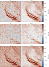Fig. 4 Results for the north patch. Top: observed dQ component (left), and reconstructed 〈SQ〉 (right). Middle and Bottom: as above but for the U and polarized intensity P components, respectively.

5 Conclusions

In this work, we have presented a multi-constrained component separation framework based on ST statistics for the recovery of polarized Galactic foregrounds from Planck data. The method reconstructs maps of polarized dust emission whose ST statistics are consistent with those expected from the Planck data, once a realization of the nuisance (noise and CMB) is added to it. These maps can be used to study the statistical properties of the dust polarized emission, or even to directly construct a ST model of this signal.

Two different sets of Q and U maps are produced: two ${\tilde{s}}_a$ maps that reproduce well the expected statistical properties, and two $\langle {\tilde{s}}_a\rangle$ maps that are a better estimate of deterministic structures, but which are slightly filtered at scales where the contamination is non-negligible. Beyond meeting the constraints of visual statistical consistency, our results show that the ${\tilde{s}}_a$ maps remain consistent across further power and cross spectra diagnostics, retaining small-scale information that is lost in the GNILC map. In the validation test, our recovered map seems to reproduce the statistical properties of the true map even at angular scales where the dust amplitude lies several orders of magnitude below the noise. We also observe that on a pixel-based comparison, the $\langle {\tilde{s}}_a\rangle$ maps seem to consistently improve on GNILC. These results demonstrate the significant potential of our approach compared to the current state of the art when applied to real data. While we are currently not able to provide uncertainties for the results produced, we note that this task has been undertaken in a parallel project (Pierre et al. 2026).

A major strength of this framework is that it is inherently flexible and can be generalized in several directions. In future work, one could extend the method to perform multifrequency component separation in polarization, thereby capturing the cross-frequency statistical dependency of Galactic dust emission. With accurate uncertainty estimates, this could enable the production of a distributions of high-quality multifrequency polarized microwave dust models. Beyond Planck, the approach could also be extended to other current and upcoming CMB datasets, such as ACT and SO. More broadly, the generality of the scattering-based formalism makes it applicable to a wide class of inverse and generative problems involving complex non-Gaussian physical fields.

Acknowledgements

We sincerely thank S. Clark, J.-M. Delouis, F. Levrier, S. Ghosh, I. Grenier, S. Mallat, and S. Pierre, for various insights and advice. The authors acknowledge Interstellar Institute’s program “II7” and the Paris-Saclay University’s Institut Pascal for hosting fruitful discussions behind this work. This work received government funding managed by the French National Research Agency under France 2030, reference numbers “ANR-23-IACL-0008” and “ANR-25-CE46-6634”. This work was granted access to the HPC resources of MesoPSL financed by the Region Ile de France and the project Equip@Meso (reference ANR-10-EQPX-29-01) of the programme Investissements d’Avenir supervised by the Agence Nationale pour la Recherche. This research used resources of the National Energy Research Scientific Computing Center (NERSC), a Department of Energy User Facility (project mp107d-2025).

References

Appendix A HEALPix pixel square patches

We extract from full sky HEALPix maps square patches centered on the centers of HEALPix pixels at resolution Nside = 4, directly as the set of healpix subpixels of each given superpixel. Although the output data are in the format of squares, there is no reprojection from the original HEALPix pixelization. The drawback is that the output square maps are “distorted”, as HEALPix pixels at Nside = 4 are not strictly-speaking “square” (even if they are in the format of a square grid). The main advantage of making “pseudo squares” that match HEALPix pixels is that we avoid any reprojection effects³.

The objective of extracting such patches is to use data processing tools designed for square images. In particular, we will make use of Fourier transforms, wavelet transforms, convolutions, and filtering on square maps. Eventually, these maps could be recombined later on into a full spherical map.

In order to avoid discontinuities, border effects, and aliasing, we add bordering pixels to each Nside = 4 superpixel (of size 512×512 for original maps at Nside = 2048). Here, we adopt 128-pixel wide borders. The dimensions of the final extracted maps is hence 768×768 pixels. The additional padding with 128-pixel wide borders allows for apodization outside of the area of interest for the patch, and taking care of border effects if when we recombine the patches into a full sky.

In contrast to the CMB, where the E and B mode decomposition is the natural language for cosmological inference, Galactic foregrounds such as thermal dust emission are best studied in terms of the Stokes parameters Q and U. Indeed, Q and U are the directly measured, local quantities that retain a simple physical interpretation: they encode the polarization amplitude and angle relative to a tangent-plane basis at each point on the sky, which are directly connected to the geometry of the Galactic magnetic field and dust grain alignment. In comparison, the E/B decomposition is intrinsically non-local, involving harmonic transforms that mix information across large regions of the sky. While this is optimal for characterizing CMB fluctuations, it obscures the local structure and non-Gaussian statistics that are crucial for understanding the physics of dust polarization. Note that for instance, the E and B fields for a single bright pixel vanish in that pixel, making IE and IB correlations equal to zero, while IQ, IU, and QU correlations are non-zero for a non-vanishing polarization fraction when none of I, Q and U vanishes.

There is, however, a practical difficulty. Working in Q and U introduces the geometric subtlety that their definition depends on the orientation of the local polarization basis, which varies across the sphere. To compare polarization measurements across pixels, it is therefore necessary to enforce a consistent choice of basis locally in the patch of interest. This is accomplished by parallel transporting the reference axes from a chosen origin (e.g. the center of a HEALPix superpixel at Nside = 4) to each pixel, thereby defining a common frame. The relative rotation angle ψ between the HEALPix convention at each pixel and the transported frame specifies how Q and U transform. Correcting for this angle reduces spurious mixing of the Stokes parameters and ensures that spatial correlations in Q and U reflect genuine astro-physical patterns rather than coordinate artifacts. In this way, parallel transport provides the geometric foundation that makes the analysis of polarized dust foregrounds in terms of Q and U both consistent and physically meaningful.

To consistently define polarization across a patch, we parallel transport a reference axis from the patch center to each pixel. Let $\widehat{\upsilon }$ be the transported reference axis and ${\widehat{e}}_{\theta }$, ${\widehat{e}}_{\text{Φ}}$ the local tangentplane basis at a pixel. The rotation angle ψ between the transported axis and the local basis is defined by projecting $\widehat{\upsilon }$ onto the local axes: $$\psi =\text{atan}\left({\widehat{e}}_{\text{Φ}}\cdot \widehat{\upsilon },{\widehat{e}}_{\theta }\cdot \widehat{\upsilon }\right)$$

This angle ψ is then used to rotate the Stokes parameters (Q, U) from the local HEALPix frame into the common, transported frame via the spin-2 transformation: $$\begin{array}{cc}{Q}^{\prime }=Q\text{\hspace{0.17em}cos}\left(2\psi \right)+U\text{\hspace{0.17em}sin}\left(2\psi \right),Q& U^{\prime }=-\end{array}Q\text{\hspace{0.17em}sin}\left(2\psi \right)+U\text{\hspace{0.17em}cos}\left(2\psi \right),$$

where Q′ and U′ represent the rotated Stokes parameters. After this rotation, all pixels in the patch share a consistent polarization frame, allowing the most meaningful comparison and analysis of Q and U across the patch.

Appendix B Input data and nuisance

We have chosen to work with the PR4 Planck NPIPE maps Akrami et al. (2020a), as they have higher signal-to-noise at intermediate scales in polarization. We process the 353 GHz frequency Q and U maps in the following way: we subtract a Wiener-filtered CMB map and convolve the maps to a common resolution of 10 arcmin. We assume that the input polarization maps have a Gaussian beam with a FWHM of 4.76 arcmin Akrami et al. (2020a). We convert the frequency maps to MJy/sr.

The nuisance maps for 353 GHz Q and U maps are the sum of noise and CMB residuals. We use the difference of simulated half-ring maps as the noise proxy, as they share the same systematics and have uncorrelated noise. We borrow 100 realizations of half-ring maps from the NPIPE simulations at NERSC⁴. CMB residual is estimated by propagating the Wiener filter coefficient to simulated CMB maps as: $$a_{{\ell }_{m_{{\text{res}}_i}}}=a_{{\ell }_{m_{{\text{CMB}}_i}}}-w{a}_{{\ell }_{m_{{\text{CMB}}_i}}}$$(B.1)

where i represents mode {T, E, B}, $a_{{\ell }_{m_{{\text{res}}_i}}}$. is the residual CMB harmonic coefficient, $a_{{\ell }_{m_{{\text{CMB}}_i}}}$ is the CMB harmonic coefficient, and w is the Wiener filter coefficient. As the 857 GHz intensity map is only used as a tracer of dust emission in cross-statistics with 353 GHz Q and U maps, and considering that its contamination by CIB and noise is expected to be independent of both signal and noise at 353 GHz, we simulate only nuisance maps for the 353 GHz Q and U maps.

Appendix C Scattering covariances

The set of summary statistics that we will use are scattering covariances. Suppose that j ∈ {0,…,J_max − 1} and $\theta \in \left\{\frac{\pi }{4},0,-\frac{\pi }{4},-\frac{\pi }{2}\right\}$ define, respectively, a dyadic scale and an orientation of a given map x, where J_max is the number of dyadic scales retained in the analysis. In this paper, we use J_max = 7. Then, λ ≡ (2^−j, θ) defines a specific oriented scale. If ψ^λ is a band-pass filter at oriented scale λ, then scattering covariances are defined as: $$\begin{array}{lll}{S}_1\left({\lambda }_1\right)\hfill & \equiv \hfill & \langle \left|x\star {\psi }^{{\lambda }_1}\right|\rangle \hfill \\ S_2\left({\lambda }_1\right)\hfill & \equiv \hfill & \langle {\left|x\star {\psi }^{{\lambda }_1}\right|}^2\rangle \hfill \\ S_3\left({\lambda }_1,{\lambda }_2\right)\hfill & \equiv \hfill & \frac{\text{Cov}\left[x\star {\psi }^{{\lambda }_2},\left|x\star {\psi }^{{\lambda }_1}\right|\star {\psi }^{{\lambda }_2}\right]}{\sqrt{\langle {\left|x\star {\psi }^{{\lambda }_1}\right|}^2\rangle }\sqrt{\langle {\left|x\star {\psi }^{{\lambda }_2}\right|}^2\rangle }}\hfill \\ S_4\left({\lambda }_1,{\lambda }_2,{\lambda }_3\right)\hfill & \equiv \hfill & \frac{\text{Cov}\left[\left|x\star {\psi }^{\lambda 1}\right|\star {\psi }^{{\lambda }_3},\left|x\star {\psi }^{{\lambda }_2}\right|\star {\psi }^{{\lambda }_3}\right]}{\sqrt{\langle {\left|x\star {\psi }^{{\lambda }_1}\right|}^2\rangle }\sqrt{\langle {\left|x\star {\psi }^{{\lambda }_2}\right|}^2\rangle }},\hfill \end{array}$$(C.1)

where ⋆ denotes a convolution, and the averages are taken over the pixel values. Therefore we can define the quantity $$\text{Φ}\left(x\right)\equiv \left\{\mu /\sigma ,\text{log}\left(S_1\right),\log \left(S_2\right),S_3,S_4\right\},$$(C.2)

where μ and σ denote the pixel-wise mean and standard deviation of x. Notice that the terms S₂, S₃, and S₄ can take two different maps x₁ and x₂ as input, for instance $S_2\left({\lambda }_1\right)=\langle \left(x_1\star {\psi }^{{\lambda }_1}\right)\left(x_2\star {\psi }^{{\lambda }_1}\right)*\rangle$ and vice versa. Therefore, we can in general write the cross-statistics maps Φ(x₁, x₂) for x₁ ≠ x₂ and define Φ(x, x) ≡ Φ(x).

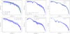Fig. B.1 Various cross spectra between the recovered maps and the expected spectra from the data. Top: Validation on the Orion region (true map indicated by sQ). Bottom: application to the North patch.

The normalization in equation is justified as follows; without the normalization, high frequency modes will be completely subdominant compared to low-frequency ones in the objective function, and so the gradient descent will be only driven by large scales. With the normalization included, a reweighting is performed such that small scales modes are not neglected.

Notice, finally, that since the logarithm is taken for the S₁ and S₂, as this definition was found to aid convergence, no normalization is required for these two terms.

The seven loss functions minimized in this work to recover the maps $\left\{{\tilde{s}}_Q,{\tilde{s}}_U\right\}$, which satisfy the constraints given in Eqs. 2–5, are defined as follows: $${ℒ}_{1,2}\left(u_a\right)=\frac{1}{M}{\displaystyle \sum _{i=1}^M{\left|\text{Φ}\left(u_a+c_{a,i}\right)-\text{Φ}\left(d_a\right)\right|}^2},$$(C.3) $${ℒ}_{3,4}\left(u_a\right)={\left|\text{Φ}\left(d_a-u_a\right)-\frac{1}{M}{\displaystyle \sum _{i=1}^M\text{Φ}\left(c_{a,i}\right)}\right|}^2,$$(C.4) $${ℒ}_5\left(u_Q,u_U\right)=\frac{1}{M}{\displaystyle \sum _{i=1}^M{\left|\text{Φ}\left(u_Q+c_{Q,i},u_U+c_{U,i}\right)-\text{Φ}\left(d_Q,d_U\right)\right|}^2},$$(C.5) $${ℒ}_{6,7}\left(u_a,d_I\right)=\frac{1}{M}{\displaystyle \sum _{i=1}^M{\left|\text{Φ}\left(u_a+c_{a,i},d_I\right)-\text{Φ}\left(d_a,d_I\right)\right|}^2},$$(C.6)

Here, a indexes the polarization channels (a ∈ {Q, U}), and M denotes the number of noise realizations used to estimate the expected scattering statistics.

Appendix D Additional figures

Figure B.1 shows the cross-spectra of the different maps for both the North patch and the Orion region. Figure D.1 compares our ${\tilde{s}}_Q$ map for the North patch with different PySM 3 models.

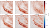Fig. D.1 Comparison of our recovered model with the corresponding PySM 3 maps for the same region. The maps ${\tilde{s}}_Q^{d9}$, ${\tilde{s}}_Q^{d10}$, and ${\tilde{s}}_Q^{d12}$ correspond to three different models provided by PySM 3: a single-modified blackbody model with fixed spectral parameters (d9), a spatially varying modified blackbody model (d10), and a six independent layers dust model, accounting for multiple dust populations (d12), respectively.

All Tables

All Figures

Fig. 1 Signal maps of the patch of interest in our work centered at (l, b) = (315, 78.): Top left: I 353 GHz. Top right: I 857 GHz. Middle left: Q 353 GHz before polarization rotation. Middle right: Q 353 GHz after polarization rotation. Bottom left: U 353 GHz before polarization rotation. Bottom right: U 353 GHz after polarization rotation. In this paper, we only used the data from the right column.

In the text

Fig. 2 Top: results of our component separation algorithm for the Stokes Q component in the rotated polarization reference frame. The map labeled dQ is the CMB-subtracted Planck map, while ${\tilde{s}}_Q$ denotes the corresponding component-separated dust emission map. For comparison, the corresponding region of the GNILC map is shown. A random realization of the nuisance component, cQ,I, has been added to the ${\tilde{s}}_Q$ map to demonstrate statistical consistency with dQ. Similarly, the recovered nuisance $d_Q-{\tilde{s}}_Q$ is compared with a random realization of the noise. In addition, we plot dQ – GNILC in order to demonstrate the existence of dust residuals in the recovered nuisance map. Finally, the residual between ${\tilde{s}}_Q$ and the corresponding GNILC map is shown. Bottom: as above, but for the high-S/N region used for validation. Note that in this case the GNILC map is filtered to facilitate comparison with the results above. Finally, in the bottom row we compare the true signal, sQ, with the average $\langle {\tilde{s}}_Q\rangle$ of ensembles obtained by using different initial conditions, as well as the residual between the true signal, sQ, and the recovered, $\langle {\tilde{s}}_Q\rangle$, and with the recovered GNILC.

In the text

Fig. 3 Top: power spectra of the maps shown in Fig. 2a. The solid blue line shows the initial Planck map dQ, while the dashed blue line (with 1σ margin) corresponds to the recovered map after adding the nuisance. The dashed purple line correspond to the recovered dust signal, ${\tilde{s}}_Q$. For comparison, the power spectrum of the true polarized dust emission is approximated by taking the cross-spectrum of the two half-ring maps (dash-dotted black line). The solid purple line corresponds to the average recovered signal $\langle {\tilde{s}}_Q\rangle$ (see Sect. 3.2). Finally, the solid and dashed green lines correspond to the nuisance (with 1σ margin) and recovered nuisance maps. For comparison, the power spectrum of the filtered GNILC map is also shown in orange. Bottom: as above, but for the maps of Fig. 2b. In this case, the power spectrum of the true polarized dust emission (solid black line) is known.

In the text

	Fig. 4 Results for the north patch. Top: observed dQ component (left), and reconstructed 〈SQ〉 (right). Middle and Bottom: as above but for the U and polarized intensity P components, respectively.
In the text

	Fig. B.1 Various cross spectra between the recovered maps and the expected spectra from the data. Top: Validation on the Orion region (true map indicated by sQ). Bottom: application to the North patch.
In the text

Fig. D.1 Comparison of our recovered model with the corresponding PySM 3 maps for the same region. The maps ${\tilde{s}}_Q^{d9}$, ${\tilde{s}}_Q^{d10}$, and ${\tilde{s}}_Q^{d12}$ correspond to three different models provided by PySM 3: a single-modified blackbody model with fixed spectral parameters (d9), a spatially varying modified blackbody model (d10), and a six independent layers dust model, accounting for multiple dust populations (d12), respectively.

In the text

References

- Akrami, Y., Andersen, K. J., Ashdown, M., et al. 2020a, A&A, 643, A42 [NASA ADS] [CrossRef] [EDP Sciences] [Google Scholar]
- Akrami, Y., Ashdown, M., Aumont, J., et al. 2020b, A&A, 641, A4 [NASA ADS] [CrossRef] [EDP Sciences] [Google Scholar]
- Allys, E., Levrier, F., Zhang, S., et al. 2019, A&A, 629, A115 [NASA ADS] [CrossRef] [EDP Sciences] [Google Scholar]
- Allys, E., Marchand, T., Cardoso, J.-F., et al. 2020, Phys. Rev. D, 102, 103506 [NASA ADS] [CrossRef] [Google Scholar]
- Auclair, C., Allys, E., Boulanger, F., et al. 2024, A&A, 681, A1 [NASA ADS] [CrossRef] [EDP Sciences] [Google Scholar]
- Bruna, J., & Mallat, S. 2013, IEEE Trans. Pattern Anal. Mach. Intell., 35, 1872 [CrossRef] [Google Scholar]
- Bruna, J., & Mallat, S. 2019, Math. Statist. Learn., 1, 257 [CrossRef] [Google Scholar]
- Cardoso, J.-F., Le Jeune, M., Delabrouille, J., Betoule, M., & Patanchon, G. 2008, IEEE J. Selected Top. Signal Process., 2, 735 [Google Scholar]
- Cheng, S., & Ménard, B. 2021, MNRAS, 507, 1012 [NASA ADS] [CrossRef] [Google Scholar]
- Cheng, S., Morel, R., Allys, E., Ménard, B., & Mallat, S. 2024, PNAS Nexus, 3, pgae103 [Google Scholar]
- Delabrouille, J., & Cardoso, J.-F. 2009, in Data Analysis in Cosmology, 665, eds. V. J. Martínez, E. Saar, E. Martínez-González, & M.-J. Pons-Bordería, 159 [NASA ADS] [CrossRef] [Google Scholar]
- Delabrouille, J., Cardoso, J.-F., & Patanchon, G. 2003, MNRAS, 346, 1089 [Google Scholar]
- Delouis, J.-M., Allys, E., Gauvrit, E., & Boulanger, F. 2022, A&A, 668, A122 [NASA ADS] [CrossRef] [EDP Sciences] [Google Scholar]
- Eriksen, H. K., Dickinson, C., Lawrence, C. R., et al. 2006, ApJ, 641, 665 [CrossRef] [Google Scholar]
- Górski, K. M., Hivon, E., Banday, A. J., et al. 2005, ApJ, 622, 759 [Google Scholar]
- Hothi, I., Allys, E., Semelin, B., & Boulanger, F. 2024, A&A, 686, A212 [NASA ADS] [CrossRef] [EDP Sciences] [Google Scholar]
- Jeffrey, N., Boulanger, F., Wandelt, B. D., et al. 2022, MNRAS, 510, L1 [Google Scholar]
- Kamionkowski, M., & Kovetz, E. D. 2016, ARA&A, 54, 227 [Google Scholar]
- Lei, M., & Clark, S. 2023, ApJ, 947, 74 [NASA ADS] [CrossRef] [Google Scholar]
- Lei, M., Clark, S. E., Morel, R., et al. 2025, Neutral gas phase distribution from HI morphology: phase separation with scattering spectra and variational autoencoders [Google Scholar]
- Martínez-Solaeche, G., Karakci, A., & Delabrouille, J. 2018, MNRAS, 476, 1310 [Google Scholar]
- Mousset, L., Allys, E., Price, M. A., et al. 2024, A&A, 691, A269 [NASA ADS] [CrossRef] [EDP Sciences] [Google Scholar]
- Nocedal, J. 1980, Math. Computat., 35, 773 [Google Scholar]
- Pierre, S., Allys, E., Richard, P., Soletskyi, R., & Tsouros, A. 2026, arXiv e-prints [arXiv:2602.05816] [Google Scholar]
- Planck Collaboration I. 2020a, A&A, 641, A1 [NASA ADS] [CrossRef] [EDP Sciences] [Google Scholar]
- Planck Collaboration XLII. 2020b, A&A, 643, A42 [NASA ADS] [CrossRef] [EDP Sciences] [Google Scholar]
- Planck Collaboration IV. 2020c, A&A, 641, A4 [NASA ADS] [CrossRef] [EDP Sciences] [Google Scholar]
- Regaldo-Saint Blancard, B., Levrier, F., Allys, E., Bellomi, E., & Boulanger, F. 2020, A&A, 642, A217 [EDP Sciences] [Google Scholar]
- Regaldo-Saint Blancard, B., Allys, E., Boulanger, F., Levrier, F., & Jeffrey, N. 2021, A&A, 649, L18 [NASA ADS] [CrossRef] [EDP Sciences] [Google Scholar]
- Remazeilles, M., Delabrouille, J., & Cardoso, J.-F. 2011, MNRAS, 418, 467 [Google Scholar]
- Siahkoohi, A., Morel, R., Balestriero, R., et al. 2023a, arXiv preprint [arXiv:2085.16189] [Google Scholar]
- Siahkoohi, A., Morel, R., Maarten, V., et al. 2023b, in International Conference on Machine Learning, PMLR, 31754 [Google Scholar]
- The Pan Experiment Group 2025, ApJ, 991, 23 [Google Scholar]
- Thorne, B., Dunkley, J., Alonso, D., & Nœss, S. 2017, MNRAS, 469, 2821 [NASA ADS] [CrossRef] [Google Scholar]
- Valogiannis, G., & Dvorkin, C. 2022, Phys. Rev. D, 105, 103534 [Google Scholar]
- Zonca, A., Thorne, B., Krachmalnicoff, N., & Borrill, J. 2021, J. Open Source Softw., 6, 3783 [NASA ADS] [CrossRef] [Google Scholar]
We used SMICA CMB maps from Planck PR3 (Akrami et al. 2020b) and the theoretical I, E, B auto- and cross-spectra to evaluate the Wiener-filtered CMB.
For more information on HEALPix, see Górski et al. (2005), or the HEALPix webpage.
The simulations can be found at NERSC:/global/cfs/cdirs/cmb/data/planck2020