


| Issue |
A&A
Volume 710, June 2026
|
|
|---|---|---|
| Article Number | A9 | |
| Number of page(s) | 20 | |
| Section | Extragalactic astronomy | |
| DOI | https://doi.org/10.1051/0004-6361/202558009 | |
| Published online | 28 May 2026 | |
BASS
LV. Connecting X-ray variability with physical properties of active galactic nuclei and a new path to cosmological distances
1
Dipartimento di Matematica e Fisica, Università degli Studi Roma Tre, via della Vasca Navale 84, I-00146 Roma, Italy
2
INAF – Osservatorio Astrofisico di Arcetri, Largo Enrico Fermi 5, I-50125 Firenze, Italy
3
INAF – Osservatorio Astronomico di Roma, Via Frascati 33, 00078 Monte Porzio Catone, Italy
4
INAF – Osservatorio di Astrofisica e Scienza dello Spazio di Bologna, Via Gobetti 93/3, I-40129 Bologna, Italy
5
Pontificia Universidad Católica de Chile, Instituto de Astrofísica, Casilla 306, Santiago 22, Chile
6
Instituto de Estudios Astrofísicos, Facultad de Ingeniería y Ciencias, Universidad Diego Portales, Av. Ejército Libertador 441 Santiago, Chile
7
Frontier Research Institute for Interdisciplinary Sciences, Tohoku University, Sendai 980-8578, Japan
8
Astronomical Institute, Tohoku University, Aramaki, Aoba-ku, Sendai, Miyagi 980-8578, Japan
9
Global Center for Science and Engineering, Faculty of Science and Engineering, Waseda University, 3-4-1 Okubo, Shinjuku, Tokyo 169-8555, Japan
10
Cahill Center for Astronomy and Astrophysics, California Institute of Technology, Pasadena, CA 91125, USA
11
Department of Physics, SRM University–AP, Amaravati 522240, India
12
Eureka Scientific, 2452 Delmer Street, Suite 100 Oakland, CA 94602-3017, USA
13
Department of Physics and Astronomy, Georgia State University, 25 Park Place, Suite 605 Atlanta, GA 30303, USA
14
Korea Astronomy and Space Science Institute, 776 Daedeokdae-ro, Yuseong-gu, Daejeon 34055, Republic of Korea
15
European Space Agency (ESA), European Space Research and Technology Centre (ESTEC), Keplerlaan 1, 2201 AZ, Noordwijk, The Netherlands
16
Department of Physics, Yale University, P.O. Box 208120 New Haven, CT 06520, USA
17
Leibniz-Institut für Astrophysik Potsdam (AIP), An der Sternwarte 16, 14482 Potsdam, Germany
18
Institute for Astronomy, University of Hawai’i, 2680 Woodlawn Drive, Honolulu, HI 96822, USA
19
Jet Propulsion Laboratory, California Institute of Technology, 4800 Oak Grove Drive, MS 169-224 Pasadena, CA 91109, USA
20
School of Physics and Astronomy, Tel Aviv University, Tel Aviv, 69978, Israel
21
Instituto de Alta Investigación, Universidad de Tarapacá, Casilla 7D, Arica, Chile
22
Yale Center for Astronomy & Astrophysics and Department of Physics, Yale University, P.O. Box 208120 New Haven, CT 06520-8120, USA
23
Department of Astronomy, University of Geneva, ch. d’Ecogia 16, 1290 Versoix, Switzerland
24
Instituto de Estudios Astrofísicos, Facultad de Ingeniería y Ciencias, Universidad Diego Portales, Av. Ejército Libertador 441 Santiago, Chile
25
Kavli Institute for Astronomy and Astrophysics, Peking University, Beijing 100871, PR China
★ Corresponding author: This email address is being protected from spambots. You need JavaScript enabled to view it.
Received:
6
November
2025
Accepted:
16
February
2026
Abstract
X-ray variability is a well-established characteristic of active galactic nuclei (AGNs) known to correlate inversely with both the supermassive black hole mass (MBH) and luminosity, although the degree of each remains a topic of debate. The potential of X-ray variability as a proxy for MBH or for intrinsic LX has led to proposals to use AGNs as standard candles to test cosmological models. However, the large intrinsic dispersion in these relations has limited their practical applications. In this work, we investigate the dependence of X-ray variability on physical properties of AGNs using a sample of 134 Seyfert 1 galaxies from the BAT AGN Spectroscopic Survey (BASS), which is the largest sample to date (it is more than three times larger than samples used in previous studies). Contrary to earlier findings, we observed that X-ray variability correlates with luminosity just as strongly as with MBH. Furthermore, we still find no evidence of the expected anti-correlation between variability and the Eddington ratio, even when using refined bolometric luminosities from Spectral Energy Distribution (SED) fitting to compute the Eddington ratio. From a cosmological perspective, the increased sample size reduces the scatter in the log L–log σNXS2 relation to ∼0.63 dex – a significant improvement over previous results, but still too large to serve as competitive standard candles, when compared to Supernovae Ia (uncertainties on distances of ∼5–10%) or the LX − LUV relation in quasars (uncertainties of 10–12%). We tested including the width of broad emission lines as additional parameters, but we found that this does not significantly lower the observed dispersion, contrary to previous studies on smaller samples. Finally, we discuss how future X-ray missions such as AXIS and NewAthena will improve this scenario by enabling precise variability measurements for thousands of AGNs up to redshift z ∼ 3.
Key words: galaxies: active / galaxies: Seyfert / distance scale
© The Authors 2026
 Open Access article, published by EDP Sciences, under the terms of the Creative Commons Attribution License (https://creativecommons.org/licenses/by/4.0), which permits unrestricted use, distribution, and reproduction in any medium, provided the original work is properly cited.
This article is published in open access under the Subscribe to Open model. This email address is being protected from spambots. You need JavaScript enabled to view it. to support open access publication.
1. Introduction
Active galactic nuclei (AGNs) are powered by accretion onto supermassive black holes (SMBHs) and are among the most luminous sources in the Universe. They are observed across the entire cosmic time, up to redshift ∼10 (Mortlock et al. 2011; Wang et al. 2021; Napolitano et al. 2025), and they play a key role in the formation and evolution of galaxies and black holes (Fabian 2012; Kormendy & Ho 2013). One of the defining features of AGNs is their variability, which is observed across the entire electromagnetic waveband, from radio to X-rays (e.g. Cristiani et al. 1996; Ulrich et al. 1997; McHardy et al. 2004). This variability occurs on a range of timescales, from hours to decades to even larger periods, and it provides a unique tool for probing the physical processes both close to and far from the central SMBH. In the X-ray band, variability is observed from very short (less than 103 s) to long (years) timescales (Uttley & McHardy 2005; McHardy et al. 2004; Peca et al. 2025; Sartori et al. 2018). It is thought to originate from processes within the innermost regions of the accretion disk and corona, making it a powerful diagnostic of the AGN structure and dynamics (Mushotzky et al. 1993; Ulrich et al. 1997; Uttley et al. 2014; Middei et al. 2017; Cackett et al. 2021; De Marco et al. 2022).
A well-established correlation exists between AGN X-ray variability amplitude and both the black hole mass (MBH) and the luminosity, with more massive, more luminous AGNs systematically showing lower variability at different wavelengths (Nandra et al. 1997; Turner et al. 1999; Lu & Yu 2001; O’Neill et al. 2005; McHardy et al. 2006; Gierliński et al. 2008; Zhou et al. 2010; Ponti et al. 2012; Kelly & Shen 2013; Tortosa et al. 2023). It has been suggested that the true physical driver of the variability is the MBH, with the relation with the luminosity emerging as a consequence, due to the dependence of luminosity on the black hole mass itself (e.g. O’Neill et al. 2005; Papadakis 2004; Ponti et al. 2012; Tortosa et al. 2023). Recent hard–X results have further shown that the amplitude of the variability, measured for example by the excess variance  , primarily anti-correlates with MBH, with no significant dependence on λEdd on ∼ 10 ks timescales (Serafinelli et al. 2024). At the same time, many studies of X-ray AGN variability have used small datasets, and the dependence of variability on MBH, luminosity, and accretion efficiency remains poorly understood.
Recent large-sample studies have further highlighted the importance of variability scaling relations at different wavelengths. Georgakakis et al. (2026) used SRG/eROSITA multi-epoch X-ray photometry to measure the ensemble excess variance for nearly ten thousand QSOs, extending the σNXS2–MBH anti-correlation to the highest black hole masses and finding non-monotonic (‘U-shaped’) dependence on the Eddington ratio. Hélias et al. (2026) analysed Gaia, Sloan Digital Sky Survery (SDSS), and Zwicky Transient Facility (ZTF) light curves for a large AGN sample and confirmed the strong link between variability timescales and black hole mass in the optical wavelengths. Dutra et al. (2025) found evidence of Evolving Dark Energy cosmological models using the relation of the variability amplitude and the characteristic timescale with the intrinsic luminosity in the optical for a sample of ∼7000 AGN from the SDSS Stripe 82 region.
The fact that AGNs are observed over the entire cosmic history makes them valuable not only for understanding SMBH growth and galaxy evolution but also as potential cosmological probes. Their brightness and ubiquity make them ideal candidates for tracing the expansion history of the Universe and testing cosmological models at both early and late epochs. Accurate distance measurements across a wide range of redshifts are essential for constraining the nature of dark energy and the geometry of the Universe (e.g. Riess et al. 1998; Perlmutter et al. 1999; Planck Collaboration V 2020). While Type Ia supernovae have been the primary standard candles up to z ∼ 2, their limited redshift reach motivates the search for complementary probes capable of extending distance measurements to the epoch of re-ionisation. In this context, AGNs offer a unique opportunity, as they are among the brightest persistent sources in the Universe. Various empirical correlations involving AGN luminosity have been explored to investigate the possible use of AGNs as standard candles. Examples include the Baldwin effect – linking the continuum luminosity to the equivalent width of broad emission lines (Baldwin 1977) – and the radius–luminosity (R–L) relation measured via reverberation mapping (RM) of the broad-line region (BLR; e.g. Watson et al. 2011; Khadka et al. 2022). While promising in concept, these correlations typically suffer from large intrinsic dispersions (up to ∼0.8 dex), which limit their utility for precise distance determinations, or they are applicable over restricted redshift ranges. Another proposed approach uses water megamaser emission to determine geometric distances (Pesce et al. 2020), but this method is constrained by the rarity of such sources and the high observational demands required for accurate measurements. A more recent and promising method exploits the tight empirical relation between the X-ray and UV luminosities in quasars (Lusso et al. 2020). Thanks to careful sample selection and correction for systematic biases, the observed dispersion has been reduced from initial values of ∼0.40 dex (Lusso & Risaliti 2016) to as low as ∼0.12 dex in the best samples (Sacchi et al. 2022), with an estimated intrinsic scatter below 0.1 dex (Signorini et al. 2024).
The anti-correlation between variability (specifically measured as the X-ray excess variance) and luminosity suggests that variability can also serve as a proxy for intrinsic luminosity (Ponti et al. 2012; La Franca et al. 2014). However, in this case, previous work has shown a high scatter in the relation, making the derived distances not particularly useful for cosmological applications. La Franca et al. (2014) studied a sample of 40 radio-quiet X-ray unobscured AGNs and found that including broad line information in the analysis significantly lowered the dispersion (see Sect. 5). In said work, including information from the full width at half maximum (FWHM) decreased the dispersion values from 1.32 dex to 0.93 dex when using Hβ and from 1.28 dex to 0.56 dex when using Paβ.
Overall, the study of X-ray variability in AGNs is key not only to understanding the physical mechanisms governing the X-ray corona and its connection with the accretion process but also to exploring its potential as a cosmological tool. For the work presented in this paper, we used the Burst Alert Telescope (BAT) AGN Spectroscopic Survey (BASS; Koss et al. 2022a) to systematically investigate X-ray variability in a sample of ∼150 objects with multi-wavelength information, significantly increasing statistics and completeness compared to previous studies. Our goals are the following:
-
To investigate the dependence of X-ray variability on physical AGN parameters such as MBH and the Eddington ratio (λEdd) while taking advantage of the recently published spectral energy distribution (SED) based estimates of λEdd (Gupta et al. 2024) and the extensive multi-wavelength characterisation of BASS.
-
To assess the reliability of using X-ray variability as a proxy for intrinsic luminosity and as a potential distance indicator, quantifying how the statistical power of the BASS sample affects the scatter in the excess variance–luminosity relation.
-
To test whether incorporating broad-line width information, following La Franca et al. (2014), can further reduce the observed dispersion.
-
To evaluate how future X-ray facilities will enhance the use of AGN variability for cosmological distance measurements.
The paper is structured as follows. In Sect. 2 we describe the sample and its properties. In Sect. 3 we describe how we performed the fits throughout the paper. In Sect. 4 we study the dependence of X-ray variability on the AGN properties, in particular the MBH, the monochromatic luminosities at different wavelengths, and the λEdd. In Sect. 5 we test the use of this sample as a calibrator for AGN distance measurement. In Sect. 6 we discuss future implementations of the method in light of upcoming new observatories, and in Sect. 7 we draw our conclusions. Throughout this paper, we consider a flat Lambda cold dark matter (ΛCDM) cosmology with H0 = 70 km s−1 Mpc−1, ΩΛ = 0.73, and Ωm = 0.27, as in Tortosa et al. (2023), from which we derived the luminosities used in this study. Correlations are considered significant when they yield p-values lower than 0.01, corresponding to ∼2.6σ under the null hypothesis of non-correlation, assuming a normal distribution. Errors are reported at the 68% confidence level or as the 16th and 84th percentiles, unless otherwise stated. Regarding the measurements of X-ray excess variance (see Sect. 2.1), we considered upper limits on the variability measurements that are consistent with zero at one sigma.
2. Sample selection and properties
The starting point of our work is the BASS sample1, constructed from X-ray–detected sources identified by the all-sky survey carried out with the Burst Alert Telescope (BAT; Barthelmy et al. 2005) aboard the Neil Gehrels Swift Observatory (Gehrels et al. 2004). BASS is a crucial survey for the local AGN census, as it probes AGNs up to Compton-thick obscuration levels (which is, with a column density of NH > 1024 cm−2; Ricci et al. 2015; Koss et al. 2016), providing a comprehensive view of accreting supermassive black holes in the nearby Universe. The Swift/BAT data (Baumgartner et al. 2013; Oh et al. 2018, 14–195 keV) is complemented with observations in the softer X-rays (0.5–10 keV) from Chandra, XMM-Newton, and NuSTAR (e.g. Ricci et al. 2017a; Peca et al. 2025). The survey also includes multi-wavelength follow-up data, from optical emission (Oh et al. 2022), to near-infrared (Ricci et al. 2022; den Brok et al. 2022, Gillette et al., in prep.), to mid- and far-IR emission observed by WISE, IRAS, Spitzer, AKARI, and Herschel (Ichikawa et al. 2017, 2019; Shimizu et al. 2017). Further insights are provided by mm/radio emission studies (Koss et al. 2021; Kawamuro et al. 2022; Ricci et al. 2023), covering the broadest possible spectral range.
The first BASS data release (DR1; Koss et al. 2017) reported MBH and X-ray properties for all 838 AGNs in the Swift/BAT 70-month catalogue (Ricci et al. 2017a). The second data release (DR2; Koss et al. 2022a) refined these results, providing more reliable and uniformly assessed MBH values for 780 unbeamed AGNs in the same catalogue. MBH were derived from broad Balmer lines and/or the RM technique for type 1 AGNs, and using maser, dynamical modelling, or velocity dispersion measurements for type 2 AGNs (Koss et al. 2022b; Mejía-Restrepo et al. 2022; Ricci et al. 2022). DR2 also calculated λEdd (Lbol/LEdd), using bolometric luminosities derived from intrinsic 14–150 keV luminosities, applying a bolometric correction factor of eight (Ricci et al. 2017a; Koss et al. 2022a).
In this work we started from the sample described in Tortosa et al. (2023), which consists of 151 radio-quiet unobscured (NH/cm−2 < 1022) type 1 AGNs from the BASS sample that had archival XMM-Newton observations and whose excess-variance has been measured by Tortosa et al. (2023, see Sect. 2.1). In addition to the X-ray variability data, we cross-matched the 151 objects with those that have optical and/or near-infrared broad-line spectral measurements from previous BASS collaboration works. This brings the sample to 144 objects with at least one measured Hydrogen broad line. For all these objects, single-epoch (SE) MBH measurements are available, with an average uncertainty of ∼0.5 dex (Koss et al. 2022a). Recent analysis of the BASS sample regards the presence of Double Peak Emission objects (Ward et al. 2025), which could be due to the emission of rotating gas in the accretion disk. The presence of these components means the broad-line widths are not directly tied to the rotational velocity of the BLR, introducing bias in virial SMBH mass estimates based on broad-line widths. Among the 144 objects with X-ray excess variance measurement and broad line measurements, ten show strong signs of being DPEs. Therefore, we removed them from the sample, as their SE MBH could be strongly affected. The final sample size is of 134 objects. Among those, 32 also have MBH estimates from RM campaigns (the ‘Reverberation mapping subsample’).
2.1. Excess variance
The excess variance is a measure of the variability amplitude in a light curve. It is calculated as the difference between the total variance of a light curve and the mean squared error, normalised by the square of the mean flux across N time bins (Nandra et al. 1997; Turner et al. 1999). Here, N represents the number of time bins within a given light curve, while xi and σi are the flux and its associated error in each interval, respectively. The excess variance is formally defined (Vaughan et al. 2003) as follows:
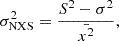 (1)
(1)
where S2 is the sample variance and σ2 is the mean squared error. The sample variance, S2, corresponds to the integral of the power spectral density (PSD) P(ν) over a given frequency range (ν1–ν2) representing the contribution to the variance from variations on timescales between 1/ν1 and 1/ν2:
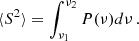 (2)
(2)
Although  is a reliable estimator of the intrinsic variance of a source, it is not free from biases. Its value depends on the integral of the PSD over specific frequencies and is influenced by several factors, including the duration of the monitoring interval, the red-noise nature of X-ray variability, and the effects of cosmological time dilation. The latter introduces dependencies on the source’s redshift (Lawrence & Papadakis 1993; Green et al. 1993; Papadakis et al. 2008; Vagnetti et al. 2011, 2016). In our sample of 134 type 1 AGNs, which consists of local AGNs (zmed = 0.035), the impact of redshift on excess variance is negligible. However, we must account for potential biases related to the varying exposure times of our observations and the red-noise character of the light curves to ensure the robustness of our results.
Tortosa et al. (2023) measured the excess variance for 153 unobscured AGNs from the BASS sample observed with XMM-Newton, using the EPIC-pn (Strüder et al. 2001) light curves, extracted using both 100 s and 1000 s binning in the 0.2–10 keV energy band, and 100 s in the 0.2–1 keV (soft), 1–3 keV (medium), and 3–10 keV (hard) energy bands (see Sect 2.2 of Tortosa et al. 2023, for more details). They selected observations that had cleaned exposure times larger than 10 ks and which had at least 10 counts in those 10 ks chunks and in each (rest frame) energy band used in the analysis, i.e. 0.2–1, 1–3, and 3–10 keV, and for each time bin of 100 s and 1000 s. This was done to avoid having too few counts in the 10 ks independent light curve to constrain the excess variance. A total of 151 sources (∼500 observations) fulfil these criteria. Of these 151 sources, 46 have upper limit measurements for the excess variance when using a 100 s bin. An object is considered an upper limit when the one-sigma uncertainty on the excess variance is equal or higher than the measured value. If an object had cleaned exposure longer than 10 ks, the light curve was split into as many 10 ks segments as possible; the excess variance was computed separately in each segment (with N time bins in each segment) and the per-segment values were then combined per source using the median. This uniform segmentation mitigates biases due to heterogeneous monitoring lengths across sources. Because the excess variance represents the integral of the PSD over the sampled frequency range, it provides a reliable proxy for variability amplitude only when that range lies entirely on one side of the PSD break. In other words, it must sample a region of the PSD with a single slope (either the low-frequency or the high-frequency part of the broken power law). Adopting the mass–accretion scaling of the PSD break (e.g. McHardy et al. 2006), the break timescale increases with black hole mass and decreases with the Eddington ratio ( , with α ≈ 1). For the BASS AGNs in our sample (MBH ≳ 106 M⊙) and moderate λEdd, the break typically occurs on timescales longer than ∼10–20 ks (see also Ludlam et al. 2015), so we are confident that we are always looking at the same PSD regime.
Regarding other possible source of biases, we note how using a fixed-length 10 ks segments for all objects ensures that the same PSD frequency range is sampled for each source, therefore mitigating the red-noise and exposure-time biases. Furthermore, Tortosa et al. (2023) find results that are consistent when using a 100 s and a 1000 s binning. Since changing the bin size by a factor of ten shifts the sampled frequency range by a factor of ten, analogous results indicate that neither high-frequency red-noise nor Poisson noise dominates the excess variance estimates.
The presence of upper limits makes it more difficult to constrain the dependence of variability on other physical properties. To start our work we looked for a way to possibly reduce the upper limits fraction with the already available data. As all of the 134 objects in our sample had at least 20 ks observations, we derived the excess variance values using extended chunks of 20 ks instead of 10 ks, as a longer light curve should be more capable to constrain variability, especially for objects with higher black hole masses, that are less variable. This choice resulted indeed in a significant decrease in the upper limit fraction with respect to the work presented in Tortosa et al. (2023). Among the 134 objects of our sample, the upper limits range from 46 to 22, which is, from 34% to 16% of the total samples. This shows how monitoring for longer times is essential for reliable variability estimates, at least for MBH > 106 M⊙. As in Tortosa et al. (2023) the excess variance values are calculated both using time bins of 100 s and 1000 s. The following results are all obtained with the 100 s binning values, but we also tested and confirmed that analogous results are obtained using time bins of 1000 s.
2.2. Emission line data
In our sample, all of the 134 objects have broad Hα and Hβ measurements from Mejía-Restrepo et al. (2022); 67 objects have Paschen lines measurements. For the broad lines Hα, Hβ, Paα, and Paβ, we have estimates of the flux and FWHM from spectral fitting. For the data coming from the previous BASS releases (Lamperti et al. 2017; den Brok et al. 2022; Mejía-Restrepo et al. 2022; Ricci et al. 2022), we refer the reader to those papers for details about the spectral fitting. Regarding the new DR3 objects, a fitting approach similar to those previous works has been adopted. More details will be available in the upcoming paper (Gillette et al., in prep.). Given the results from the spectral fitting, we only included in the analysis those objects for which the flux and FWHM could be fully constrained (i.e. we removed upper limits), and we considered only objects flagged as having a satisfactory fit. This leaves us with 115 objects with Hα, 88 objects with Hβ, 46 objects with Paα, and 50 objects with Paβ measurements.
2.3. Eddington ratio
It is our interest to study the relation between excess variance and Eddington ratio (see Sect. 4). In this work, we take advantage of the λEdd published by Gupta et al. (2024), where the SED fitting was used to derive the bolometric luminosity, instead of using a bolometric correction on monochromatic luminosity. Thanks to the extensive multi-wavelength data of the BASS sample, it was possible to obtain a bolometric luminosity from SED fitting for 115 out of the 134 objects in our sample. The missing objects are those for which the UVOT monitoring was insufficient, so the disk model could not be constrained (Gupta et al. 2024). As the SED fitting takes into account the multi-wavelength information, instead of the correction on a monochromatic luminosity, we argue that these values can be considered to be more reliable in the final estimate of the λEdd of our sources. The second ingredient to derive the λEdd is the MBH. For our sample, this estimate is obtained with SE measurements using the Hβ line for 102 objects, while 32 have MBH estimates coming from RM. In cases where RM values were available, we prioritised their use due to their higher reliability. Overall, the objects in our sample span in λEdd from ∼0.005 to ∼1.
3. Data fitting
Throughout this study, we aim to fit log-linear relations between the X-ray excess variance and other physical quantities of the AGNs in our sample. The fitting process is complicated by several challenges: (i) the presence of upper limits, (ii) significant uncertainties on both the dependent and independent variables, and (iii) asymmetric uncertainties. Importantly, our measurement uncertainties are first estimated in linear units; when transformed to logarithmic space, the upper and lower errors become asymmetric. Consequently, simply averaging upper and lower errors to define the weights would bias the fit; instead, we adopt an iterative scheme that assigns the appropriate upper or lower uncertainty to each point relative to a provisional best-fit line, and we validate this approach with mock datasets (Appendix A). To ensure the reliability of our fitting method, we validated it extensively using mock datasets specifically designed to mimic the statistical properties of our sample (see Appendix A for details). These mock tests allowed us to evaluate the method’s ability to recover the true underlying relations, meaning the values of the slope and the intercept, under varying fractions of upper limits and uncertainty configurations. Our final fitting approach is iterative. Initially, we perform a simple fit using the lmfit Python library (Newville et al. 2014) with a linear model y = a ⋅ x + b, considering as weight for each point the average uncertainty on both x and y, calculated as the mean of the upper and lower uncertainties. This preliminary fit provides a temporary best-fit line. Next, we classify each data point as lying above or below this line and, based on this classification, assign the upper or lower uncertainties to both the x and y axes. This process is repeated iteratively, with the fit recalculated at each step, until the best-fit parameters converge to a stable solution. Uncertainties are then derived on the best-fit values of the slope and the intercept with a bootstrap procedure. We validated this iterative method using mock datasets and found it to be robust for cases where the fraction of upper limits is below 30%. Given that our sample includes only 16% upper limits, we are confident on the reliability of our results. We also always performed the fit, centring the data, which is subtracting the mean values on x and y to minimise the covariance between the obtained slope and intercept of the linear fit. The mean values are then added to the best fit value of the intercept b to recover the true value.
4. Dependence on AGN physical properties
4.1. Black hole mass
We first investigated the relationship between the X-ray excess variance and the black hole mass:
 (3)
(3)
where –2.99 and 7.54 are the mean values for log(σ100 s, 20 ks2) and log(MBH), respectively. The best-fit parameters are a slope of a = −0.79 ± 0.11 and an intercept of b′= − 0.18 ± 0.07 (see Table 1). The relation is statistically significant, with 1 − p-value > 0.99. The total observed scatter around the best-fit relation is δ = 0.77 dex, which we calculated using only the detections (i.e. excluding upper limits). Figure 1 shows the best-fit relation, along with the median values of σNXS2 in five MBH bins, added to guide the eye. Some of the total scatter is due to the uncertainties on the excess variance and black hole mass values. To estimate how much of the observed scatter can be attributed to measurement uncertainties, we computed the expected uncertainty contribution as  , where δlog σ2 and δlog MBH are the mean uncertainties on the excess variance and black hole mass, respectively. The remaining scatter can be interpreted as an intrinsic component of the relation
  . However, the black hole masses used in this work were obtained using the virial equation, with most of the sample having SE mass measurements, and 32 objects having RM measurements. In both SE and RM cases, black hole masses are derived using the virial relation,
 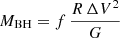 , where R is the radius of the BLR, ΔV is the velocity width of the broad emission line, and f is the virial factor, a dimensionless scaling coefficient that accounts for the geometry, kinematics, and inclination of the BLR. The velocity ΔV is usually estimated from the FWHM or the line dispersion of broad permitted lines observed in the rest-frame ultraviolet (e.g. Mg II and C IV), optical (e.g. Hβ and Hα), or near-infrared (e.g. Paβ and Paα) spectral regions (see e.g. Greene & Ho 2005; Trakhtenbrot & Netzer 2012; Shen 2013; Ricci et al. 2017b). In RM-based mass measurements, R is measured directly as the light-travel time delay (lag) between variability in the AGN continuum and the response in the broad emission lines (e.g. Bentz et al. 2009). In SE estimates, R is inferred from the AGN monochromatic luminosity using the empirical radius–luminosity (R–L) relation (e.g. Kaspi et al. 2000; Bentz et al. 2013), which is calibrated using RM samples. A major source of systematic uncertainty in both SE and RM mass estimates is the virial factor f, which reflects assumptions about the BLR structure and its orientation relative to the observer. For example, Ricci et al. (2022) reports an anticorrelation of the virial factor f with the virial mass (likely tracing an underlying anticorrelation with the observed FWHM), as expected if line widths broaden with increasing inclination in a disk-like BLR. The value of f cannot be measured directly for individual objects and is instead calibrated statistically by matching RM-based AGN black hole masses to the MBH–σ∗ relation observed in quiescent galaxies (e.g. Onken et al. 2004; Bennert et al. 2011; Woo et al. 2015). However, the true value of f may vary substantially across the AGN population due to differences in BLR inclination, turbulence, radiation pressure, and the presence of outflows or inflows (Collin et al. 2006; Mejía-Restrepo et al. 2018; Pancoast et al. 2014). This introduces an intrinsic uncertainty in mass estimates, typically not captured by the quoted measurement errors. In the case of SE estimators, additional scatter arises from the use of the R–L relation, which carries its own intrinsic dispersion of ∼ 0.13 dex (Bentz et al. 2013). Since this relation is empirically derived from RM samples, it assumes that the BLR structure and ionising continuum shape of the SE objects are similar to those in the RM sample – an assumption that may break down for sources with significantly different accretion properties, luminosities, or BLR conditions. These effects contribute to a total population-level uncertainty in virial masses of up to 0.4–0.5 dex (Wandel et al. 1999; Vestergaard & Peterson 2006; Marziani & Sulentic 2012; Landt et al. 2013; Shen 2013; Shen & Ho 2014), which is significantly larger than formal statistical uncertainties, which typically only account for errors in luminosity and line width. These systematic uncertainties in the black hole mass estimates inevitably contribute to the observed scatter in the excess variance–mass relation, and should be taken into account when interpreting its parameters. This means that part of the observed δint is still due to this intrinsic mass uncertainty. If we take a value of 0.50 dex for this additional scatter and propagate it through the slope of the best-fit relation, the intrinsic dispersion in the excess variance not attributable to black hole mass uncertainties becomes

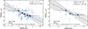 |
Fig. 1. Left: Relation between the 2–10 keV excess variance (σNXS2) (obtained with time bins of 100 s) and the black hole mass (MBH) for the sample of 134 objects. Filled cyan circles show full detections; red down-pointing triangles show upper limits; the grey shaded area shows the confidence interval at 1σ for the best-fit log-linear relation. Blue stars represent the median value of the MBH and the excess variance in six MBH bins, chosen so that in each bin there are at least 20 objects. Blue error bars indicate the bin width. Blue stars are placed solely to guide the eye, as the fit is performed on the entire sample. The p-value of the relation and the total scatter δtot are displayed, together with the best fit result. The best fit is reported on the plot as |




Fitting results for different relations.
If we consider 0.40 dex instead, we obtain δtrue ∼ 0.68 dex. We note that this 0.65–0.68 dex range is only an order of magnitude estimate, as the 0.40–0.50 dex scatter is an average value across AGN populations. The derived best-fit parameters for the σ − MBH relation are consistent with the results of Tortosa et al. (2023), as expected given the similarity between the samples, with the present work including fewer upper limits.
Our findings are also consistent with recent ensemble-variability results at longer (∼years) timescales. Georgakakis et al. (2026) reported, for a sample of ∼10 000 objects with eROSITA multi-epoch light curves, a clear decrease of the ensemble normalised excess variance with increasing MBH on rest-frame timescales of months to years. Although their methodology and timescale regime differ from the short-timescale excess variance probed in this work, the persistence of the σNXS2–MBH anti-correlation across different regimes reinforces the robustness of the physical connection between black hole mass and X-ray variability amplitude.
In Sect. 2 we described the removal of 10 objects from the sample due to strong evidence of DPE features in their Hβ lines as discussed in Ward et al. (2025), which could bias MBH estimates. To verify whether these objects are genuine outliers, we repeated the fit with the full sample, including the DPE-flagged objects. The scatter of the subsample was found to be δ = 0.89 dex. This corroborates their removal, as likely their masses are unreliable.
We also tested the relation between the excess variance and the MBH restricting it to the RM sample, which is shown on the right panel of Fig. 1. The slope we obtain is steeper than for the whole sample, but still consistent within uncertainties. Similar results were found by Tortosa et al. (2023, see their Sect. 3.2). Although RM masses are more reliable, the sample size is less than one-third when compared to the whole sample, which contributes to the overall higher uncertainties in the relation parameters estimates, although uncertainties on MBH are smaller. Future more homogeneous RM datasets will allow for more robust comparison. For the purposes of this work, the RM-only and full-sample relations are statistically consistent, and the inclusion of the RM-only result does not alter our conclusions.
4.2. Luminosity
We explored the relationship between the X-ray excess variance and intrinsic luminosity, testing the 2–10 keV X-ray luminosity and the monochromatic optical luminosities at 5100 Å and 6200 Å. The 2–10 keV X-ray luminosities are from the Ricci et al. (2017a) catalogue, where they are derived from X-ray spectral fitting. The results are summarised in Table 1 and illustrated in Fig. 2. The best-fit parameters for the 2–10 keV luminosity are consistent with the findings of Tortosa et al. (2023), as expected. Interestingly, the slopes derived for the optical luminosities are flatter compared to those for the X-ray luminosity, although they are consistent within 1σ. This is indeed expected given the well-known nonlinear relation between the X-ray and the UV luminosities in AGNs (e.g. Tananbaum et al. 1979; Vignali et al. 2003; Lusso et al. 2010). The total dispersion values range from δ = 0.73 dex to δ = 0.78 dex, with intrinsic scatter values similar to those obtained for the MBH relation, approximately δint ∼ 0.70 dex.
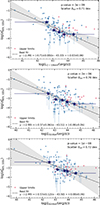 |
Fig. 2. Relation between the 2–10 keV excess variance (obtained with time bins of 100 s) and different monochromatic luminosities. The legend is the same as in Fig. 1. Top: Relation obtained using the 2–10 keV monochromatic luminosity. Middle: Relation obtained using the 5100 Å monochromatic luminosity. Bottom: Relation obtained using the 6200 Å monochromatic luminosity. Sample size N = 134. |
We compare our results with those of La Franca et al. (2014), who investigated the relationship between the excess variance and luminosity in both the X-ray (2–10 keV) and optical (5100 Å) bands. Their work employed a sample of 40 objects from Ponti et al. (2012), with no upper limits, and with distribution in redshift (0< z < 0.3) and 2–10 keV luminosities (log(L2−10 keV/erg s−1) ∼ 40 − 45) analogous to those of the BASS sample. They fitted the relation log(L) = a′⋅log(σ2)+b′, obtaining slopes of a′2 − 10 keV = −1.67 and  . These results are consistent with ours, as the slope in our formulation (a) is the reciprocal of their slope (a′). Specifically, 1/( − 1.67)∼ − 0.60 and 1/( − 1.98)∼ − 0.51. So, the increased statistics of the BASS samples still provide results consistent with the previous ones in the literature. Regarding the dispersion of the relation, we focus on this topic in Sect. 5.
4.3. The main driver of X-ray variability
Identifying the primary driver of AGN X-ray variability is key to understanding the underlying physical mechanisms. Both black hole mass and luminosity are known to correlate with the X-ray excess variance, but determining which of the two plays a more fundamental role remains an open question. One possible approach is to compare the intrinsic scatter of the two relations: a lower scatter can indicate a tighter, possibly more physically rooted correlation. This is indeed how previous works have suggested that the main driver of X-ray variability is the MBH, with the relation with the luminosity being a consequence of it (e.g. Ponti et al. 2012). In our sample, we find that the total observed scatter in the σ2–MBH relation (δ = 0.77 dex) is consistent with that in the σ2–L relation (ranging from δ = 0.73 to 0.76 dex). However, this comparison is complicated by the nature of the black hole mass estimates, which are primarily based on single-epoch virial methods. As discussed in the previous section, when we account for this additional scatter, we find that the intrinsic scatter in the σ2–MBH relation drops to ∼0.65–0.68 dex, thus becoming comparable to or even smaller than that of the luminosity-based relation. This gives hint that, despite the larger observed dispersion, black hole mass may still be more fundamentally linked to variability, and the higher scatter is, at least in part, an artefact of mass measurement uncertainties. Additional information can come from the value of the slopes, as the steepness of the relation can indicate how rapidly the variability amplitude responds to changes in each predictor. In our sample, the best-fit slopes in the log σ2–log MBH and log σ2–log L2 − 10 keV relations are comparable within 1σ (Table 1), suggesting similar response strengths. In the RM-only subset, the log σ2–log MBH slope is steeper, yet still consistent within uncertainties. In the RM-only subset, the log σ2–log MBH slope is steeper, yet still consistent, within uncertainties, with the whole sample. To further disentangle the contributions of MBH and L, we performed a residual analysis. This method tests whether one parameter adds predictive power beyond what is already explained by the other. Specifically, if the residuals of the log(σ2)–log(L2 − 10 keV) relation correlate with log(MBH), it would imply that MBH captures additional variability-related information not encoded in luminosity alone.
We first computed the residuals from the log(σ2)–log(L2 − 10 keV) best-fit relation and regressed them against log(MBH), obtaining a p-value of 0.88 and slope of α = −0.10 ± 0.06. The trend is consistent with zero at a 2σ level, while the high p-value tells us that there is no significant trend. The residuals from the log(σ2)–log(MBH) relation show no dependence on log(L2 − 10 keV), with a p-value 0.75 and a slope of α = −0.06 ± 0.08. Again, the high p-value obtained here can be considered as proof against the presence of a significant trend in the residuals. These results are shown in the upper panels of Fig. 3. We also performed the same analysis but restricted to the RM-only sample, as shown in the lower panels of Fig. 3. The analysis shows weak trends (∼2σ) in opposite directions depending on which variable is held fixed. The trend with MBH residuals is slightly more significant, at a 2.3σ level. This would suggest the MBH as the more relevant driver, but the result is only marginal.
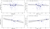 |
Fig. 3. Residual analysis to assess whether black hole mass or luminosity more fundamentally drives X-ray excess variance. Upper left: Residuals from the best fit of the log(σ2)–log(L2 − 10 keV) relation plotted against log(MBH). A weak trend can be observed (α = −0.10 ± 0.06), but the obtained p-value is 0.88, against the significance of the trend. Upper right: Residuals from the log(σ2)–log(MBH) relation plotted against log(L2 − 10 keV). There is no significant trend (α = −0.06 ± 0.08), and the p-value is 0.75. These findings suggest that for this dataset, neither MBH nor L can be considered the ‘main driver’ of the variability against the other. Lower left: Same as in the upper-left panel but restricted to the RM-only sample. A 2.3σ significant negative dependence on MBH is observed. Lower right: Same as in the upper-right panel but restricted to the RM-only sample. A 2σ positive dependence on luminosity is observed. This marginally suggests that MBH is more predictive than the luminosity. |
Taken together, the results on the scatter and the slight trend in log(σ2)–log(L2 − 10 keV) residuals may suggest that MBH is more closely related to the physical mechanism driving X-ray variability than luminosity. However, the statistical evidence remains very tentative. Ultimately, these findings highlight the importance of improving black hole mass measurements in large AGN samples. Future studies based on RM or improved calibrations of virial estimators, especially those accounting for systematic dependencies of the virial factor, will be critical for resolving the relative contributions of mass and luminosity in determining AGN variability (e.g. Villafaña et al. 2023, 2024).
4.4. Eddington ratio
The relationship between the X-ray excess variance and the λEdd is of significant interest, as it can provide insight into the variability properties of AGNs. According to McHardy et al. (2006), the break timescale in the PSD increases with MBH and decreases with increasing λEdd. If AGNs follow a universal PSD characterised by a single break frequency dependent on MBH, combined with a constant normalisation on long timescales, one would expect the strength of the relations σ2 versus MBH and σ2 versus λEdd to be comparable (Sartori et al. 2018). This would predict higher short-timescale variability for AGNs with lower MBH and higher λEdd. However, many studies have not identified a significant correlation between variability and the λEdd. For example, O’Neill et al. (2005), Gierliński et al. (2008), Zhou et al. (2010), Ponti et al. (2012), and Lanzuisi et al. (2014) reported no robust evidence of such a relationship. Similarly, for the BASS sample, Tortosa et al. (2023) found no statistically significant correlation. In this work, we aim to re-examine this relationship under updated conditions that differ from Tortosa et al. (2023). First, our sample includes fewer upper limits, which should increase the sensitivity to any underlying relation. Second, we removed objects exhibiting signs of DPE in the Hβ lines, as these objects likely have biased MBH estimates, which would propagate to their λEdd estimates. Finally, we now use λEdd values derived from bolometric luminosities obtained through SED fitting (Gupta et al. 2024). We tested the relation
 (4)
(4)
where –2.99 and –1.27 are the mean values of log(σ100 s, 2 − 10 keV2) and log(λEdd), respectively, and performed the fit as discussed in Sect. 3. The results are shown in the left panel of Fig. 4. For visualisation purposes, we added blue stars representing the median λEdd values in four bins, spaced to ensure that each bin contains at least 20 objects. The p-value of the correlation is 0.16, and the best-fit slope is a = −0.14 ± 0.15, consistent with zero, indicating that the relationship is not significant. Therefore, even with this improved sample, including fewer upper limits and updated λEdd values, we still find no evidence of a significant correlation between excess variance and the λEdd.
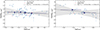 |
Fig. 4. Relation between the X-ray excess variance σNXS and the λEdd. Blue stars represent averaged bins in the Eddington ratio and are shown to guide the eye. Left: Fit performed for the whole sample, where 102 objects out of 134 have black hole masses estimated using the virial equation and 32 have RM estimates. Despite the reduced fraction of upper limits and increased precision of the λEdd estimates compared with other studies, there is still no significant relation between X-ray variability and the λEdd. Right: Same analysis for the subsample of objects with black hole masses derived from RM (N = 32). There is an anti-correlation, but it is only slightly significant. |
It is still possible that the relationship is weak but exists, hidden by large uncertainties, again mainly due to black hole mass estimates. To mitigate this, we restricted our analysis to a subset of 32 objects with MBH obtained via RM, which are considered more accurate than single-epoch mass measurements. For this subset, we fit the same relation as above, and the results are shown in the right panel of Fig. 4. The slope in this case is a = −0.53 ± 0.36, with a p-value of 0.003, indicating a statistically significant, though weak, correlation. Despite the statistical significance, this result should be interpreted with caution. The subsample of RM objects is small and may not be fully representative of the broader AGN population. Objects targeted for RM campaigns are often less massive and exhibit greater variability, as this increases the likelihood of detecting time lags and enabling MBH measurements during the monitoring campaign. For our sample, the difference in mean MBH is modest, with ⟨log(MBH/M⊙)⟩ = 7.6 ± 0.8 for non-RM objects and ⟨log(MBH/M⊙)⟩ = 7.4 ± 0.8 for RM objects. Nevertheless, this difference could still contribute to the observed discrepancy. Further studies with larger, unbiased samples with robust MBH and λEdd are required to clarify the nature of the relationship between excess variance and λEdd. As an additional test, we also explored the relation between the excess variance and the ‘X-ray Eddington ratio’, LX/LEdd, as shown in Appendix C. This quantity can in principle offer further insight into how variability depends on the relative strength of the X-ray emission. However, the correlation is only marginally significant, and strong degeneracies with black hole mass and luminosity are likely at play. For these reasons, and to avoid over-interpreting the result, we present the full discussion in the appendix.
5. Cosmological implementation
Motivated by the established link between X-ray excess variance and luminosity, we tested whether AGN variability can serve as a distance indicator. Because log(σ100 s, 20 ks2) can, in principle, provide a cosmology-independent estimate of intrinsic luminosity, this approach could extend standard-candle work beyond the redshift reach of Type Ia supernovae. In this section we evaluate this idea using the BASS sample, inverting the perspective adopted above: rather than treating log(σ100 s, 20 ks2) as the dependent variable, we use it as the predictor of intrinsic luminosity. Therefore, we treated luminosity as the dependent variable in the relation
 (5)
(5)
We attempted to fit the different luminosities in Eq. (5): the 2–10 keV luminosity, the monochromatic 5100 Å luminosity and the 4400 Å luminosity. We found that using X-ray luminosities gave the best proxy for the excess variance, with the 2–10 keV luminosity showing the lowest scatter (0.63 dex), compared to 0.70 dex and 0.72 dex for the 4400 Å and 5100 Å luminosities. This difference can be explained by the fact that the X-ray and optical observations of the sample were not simultaneous. As AGN emission can vary on short timescales, it could be that the X-ray corona state was different when optical observations were performed. The 2–10 keV luminosity is more directly tied to the X-ray excess variance as it is measured from the same observation. Note that the dispersion in this inverse relation is not directly comparable to the scatter discussed earlier and presented in Table 1. For cosmological purposes, we focus on the relation with X-ray luminosity, which has the lowest scatter. The found total scatter of 0.63 dex in the log(L2 − 10 keV)−log(σ100 s, 20 ks2) relation, which is substantially lower than the 1.33 dex reported by La Franca et al. (2014). We note that the sample in La Franca et al. (2014) has analogous distribution in redshift, MBH and luminosity as the BASS sample of this work. The reduced scatter is likely due to both the larger sample size (134 vs 40 sources) and improved completeness. This reduction is crucial, as the dispersion directly limits the precision of distance estimates derived from this relation.
Given an estimate of the intrinsic luminosity from Eq. (5), we computed the luminosity distance using
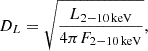 (6)
(6)
where F2 − 10 keV is the observed flux. Propagating the uncertainty on L through this relation gives the uncertainty on the luminosity distance:  .
.
In linear terms, this corresponds to a fractional uncertainty:
 (7)
(7)
This is a substantial improvement over previous results, but it is still larger than the uncertainties achievable with other cosmological probes. For reference, Type Ia supernovae typically yield 5–10% uncertainties, while quasar-based LX–LUV relations can achieve 12–20% (Lusso et al. 2020; Signorini et al. 2023).
La Franca et al. (2014) proposed a strategy to reduce the scatter in variability-based luminosity estimates by including the FWHM of broad emission lines. The idea is based on the virial relation: 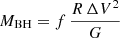 , and on the assumption that black hole mass is a fundamental driver of variability. If true, including line width could help recover this deeper physical link and reduce dispersion. In their work, La Franca et al. (2014) found that the relation
 (8)
(8)
yielded a smaller dispersion than Eq. (5) alone. In our sample, however, the variability–mass and variability–luminosity relations show comparable observed scatters, as discussed in Sect. 4. This suggests that the variability is not more fundamentally linked to mass than to luminosity, at least within our sample. Consequently, we do not expect significant improvements by including FWHM in the luminosity prediction.
For completeness, and to enable direct comparison with La Franca et al. (2014), we repeated their analysis on our larger sample. The results are presented in Appendix B. We find no reduction in scatter when using the line widths of Hα or Hβ. A moderate decrease is observed when using Paα and Paβ, but the sample sizes remain limited (N = 40 for Paα, N = 51 for Paβ). The inclusion of FWHM may be effective only when the initial dispersion is large; in our case, the already reduced scatter from sample improvements may leave little room for further improvement. As a proof of concept, we show the Hubble diagram of the BASS sample in Fig. 5. Objects are shown in light grey; dark orange points are the mean values of the luminosity distances when dividing the sample into nine bins of equal size. For a comparison, the distance values for SNIa from the Pantheon+ sample (Scolnic et al. 2022) are shown in cyan, and the shape of the Hubble diagram predicted by a flat ΛCDM model is shown in solid black. Clearly, the limited redshift range and statistics of the BASS sample make it a worse probe than SNIa for measuring cosmological distances. However, AGNs can be observed at much higher redshifts than SNIa, and future X-ray observatories could be of great importance for measuring distance using X-ray variability, as discussed in the next section.
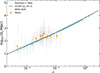 |
Fig. 5. Proof-of-concept Hubble diagram for the BASS sample (grey points) using the relation between X-ray excess variance and the 2–10 keV luminosity. The dark orange points show the mean values obtained by binning the sample into nine equal-sized bins. Cyan points represent the Pantheon+ Supernovae Ia sample (Scolnic et al. 2018), while the black line represents the prediction from a standard flat ΛCDM model. The redshift range and limited statistics of the BASS sample currently undermine the cosmological implementation of the method, but future probes might open new possibilities (see Sect. 6). |
6. Future observatories
The current results on the relation between X-ray excess variance and luminosity still exhibit significant dispersion, limiting their immediate use as a cosmological distance indicator (and therefore as a means to distinguish between cosmological models). However, future X-ray observatories will dramatically increase the number of AGNs with precise excess variance measurements, enabling tighter calibrations of this relation and its cosmological implementation.
The Advanced X-ray Imaging Satellite (AXIS)2 (Reynolds et al. 2023), a NASA concept currently in Phase A, will provide sub-arcsecond imaging with a large effective area and field of view, ideal for serendipitous AGN variability studies. NewAthena (Cruise et al. 2025), ESA next-generation X-ray observatory expected to be adopted by 2027, will host the Wide Field Imager featuring a 40′×40′ field of view and an energy resolution of < 170 eV at 7 keV, and will offer a resolving power comparable to XMM-Newton but with a considerably larger collecting area3. Both missions will therefore open a new regime for precision AGN variability measurements.
To estimate how many AGNs could be used as cosmological probes with these missions, we start from the 100 deg2 mock AGN population of Gilli et al. (2007), which represents a realistic census of sources over a wide redshift and luminosity range and also accounts for the expected fraction of AGNs that would be obscured. We then apply our selection criteria to identify objects that could be observed either by AXIS or NewAthena, and that would yield reliable X-ray excess variance measurements. For AXIS, we consider the entire 100 deg2 mock field as a realistic proxy for all serendipitous AGNs that will accumulate over the mission lifetime. For NewAthena, the current observational strategy includes 70 pointings of 200 ks and 30 pointings of 300 ks each (private communication, NewAthena team). It has not been decided yet exactly which fields will be covered by these surveys, but the total would amount to a sky area of 44 deg2. We therefore consider the numbers from the 100 deg2 catalogue multiplied by 0.44.
As shown in our BASS sample, at least 40 counts in the rest-frame 2–10 keV band over a 20 ks observation are required to obtain a robust measurement of the excess variance. Because of cosmological time dilation, a rest-frame 20 ks observation corresponds to 20 ks × (1 + z) in the observed frame, and we therefore require each object to have a total exposure of 20 ks (1 + z) and at least 40 (1 + z) counts. For NewAthena, the long planned exposures easily satisfy this condition even at the highest redshifts. For AXIS, although some serendipitous fields may have shorter exposures, the mission’s expected lifetime and cumulative coverage make it plausible that more than 100 deg2 will eventually be observed to sufficient depth. Given AXIS and NewAthena energy ranges, that are of 0.3–10 keV and 0.2–15 keV respectively, the rest-frame 2–10 keV band will be directly observed for all objects in the redshift range 0 < z < 5.7 for AXIS and 0 < z < 9 for NewAthena.
We then use the latest response matrices for both telescopes through WEBPIMMS4 to convert the 2–10 keV flux into count rate for an unobscured AGN with a photon index Γ = 1.8. We apply these conversions to the 100 deg2 mock catalogue, selecting only sources that are unobscured, which means with a column density of log(NH/cm−2) < 21, and bright enough to give a reliable X-ray excess variance measurement. We performed simulations over a photon index range of ∼1.7 − 2.0, which is reasonable for unobscured AGNs, and obtained results similar to those obtained. For simplicity, we discuss the results for the Γ = 1.8 prescription.
We also needed these objects to have a reliable spectroscopic redshift measurement. This step is crucial for the cosmological application, as reliable distances can only be derived when both variability and redshift are measured. For the sake of this exercise, we considered how many will have a detectable emission line with Euclid, the ESA space mission designed to map the geometry of the dark Universe using weak lensing and galaxy clustering (Laureijs et al. 2011). Euclid is equipped with two instruments, VIS (Euclid Collaboration: Cropper et al. 2025) and the Near-Infrared Spectrometer and Photometer (NISP-S and NISP-P; Euclid Collaboration: Jahnke et al. 2025). Over its 6-year survey duration, it will map about one-third of the extragalactic sky in the Euclid Wide Survey (EWS; Euclid Collaboration: Scaramella et al. 2022). During the EWS, slitless spectroscopic data will be acquired by NISP-S using the red grism RGE, covering 1206–1892 nm. This wavelength range enables the detection of Hα at redshifts between ∼0.84 and ∼1.9, and Hβ between ∼1.9 and ∼2.9. From the Euclid Collaboration: Lusso et al. (2024) catalogue, the flux limit for detecting Hα with Euclid is approximately 5 × 10⁻¹⁶ erg cm−2 s−1. Using the correlation from Panessa et al. (2006), we estimate that this corresponds to a 2–10 keV flux limit of ∼5 × 10⁻¹⁵ erg cm−2 s−1. The expected Hβ/Hα flux ratio for AGNs has a wide range; as discussed in Mejía-Restrepo et al. (2022), it can vary between 0.3 to 0.9, with an average of ∼0.5 for Seyfert 1 galaxies. Considering a worst-case scenario, we require objects in the redshift range 1.9–2.9 to have at least 3 times the required flux for the Hα measurement. We apply these criteria to the objects in the Gilli et al. (2007) 100 deg2 catalogue.
To sum up, we required our object to be (i) bright enough to provide a reliable X-ray excess variance measurement in the 2–10 keV range, (ii) unobscured, (iii) bright enough to obtain a reliable redshift measurement using Euclid, and (iv) in the redshift range 0.88 < z < 2.9 so that the redshift could be provided using Hα or Hβ. We find a total of ∼4500 AGNs that would satisfy the requirements for AXIS (considering serendipitous sources over the mission lifetime, for 100 deg2), and ∼3000 for the planned surveys of NewAthena (for a total of 44 deg2).
This sample size allows for binning in redshift while maintaining adequate statistics per bin. Within a narrow redshift bin, the spread in luminosity distance is small, allowing us to average over the bin to reduce the scatter. Dividing the redshift range 0.84 < z < 2.9 into 9 bins evenly spaced in log z, we find that each bin contains between 80 and 700 sources for the AXIS sample, and between 40 and 500 sources for the NewAthena one. For reference, based on the fit presented in Sect. 5, we have δlog(DL)∼0.5 dex. Assuming the uncertainty in flux is negligible, the uncertainty in the average log DL for a bin with N AGNs is reduced by a factor of  . This reduces the uncertainty on log(DL) in each bin down to between 0.02 and 0.08 dex.
In Fig. 6 we present the resulting Hubble diagrams for AXIS (left) and NewAthena (right). The AGN data points, colour-coded by whether Euclid would observe Hα or Hβ, are compared with Type Ia supernovae from the Pantheon+ compilation. We also show predictions for the ΛCDM model and two alternative cosmologies, namely a ΛCDM with a different mass parameter (Ωm = 0.1), and a w0wa model where dark matter is assumed to be varying with w = w0 = wa(1 + z). The divergence among models becomes significant only at z ≳ 2, highlighting the importance of high-redshift standard candles. While Type Ia supernovae are scarce beyond z ∼ 1.5, AGNs are more abundant in this regime, making them promising tools for future cosmological studies. As shown, a sample of thousands of objects would allow us to distinguish between cosmological models at high redshift. While the uncertainties increase at the highest redshifts, combining AGNs with other cosmological probes in this range would allow for discrimination among cosmological models.
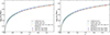 |
Fig. 6. Left: Simulated Hubble diagram obtained using the relation between X-ray excess variance and 2–10 keV luminosity to derive the luminosity distance, DL, for sources expected to be observed by AXIS (to measure variability) and Euclid (to provide spectroscopic redshifts). Right: Same simulation but for NewAthena, considering its planned deep survey coverage. The light cyan points represent the luminosity distances obtained from SNe Ia in the Pantheon+ sample. The solid, dashed, and dot–dashed black curves correspond to different cosmological models, which overlap at low redshift but diverge at z ≳ 2, where AGNs become valuable standardisable candles. |
Such increased statistics obtained by combining Euclid with AXIS and/or NewAthena allow us to perform multiple additional tests. First, we can test if there are redshift variations in the relation. This is relevant for understanding the physics of variability, but also for validating the cosmological implementation. We can also further test the relation by dividing the sample into groups based on other quantities, such as luminosity or λEdd, and examine whether the relation changes. Though encouraging, the results in Fig. 6 have some caveats. As we do not have a systematic study of the relation at higher redshift, it might be that the relation changes, the dispersion changes, or both. Furthermore, we assume that the intrinsic systematic scatter in the correlation is small and that the statistical scatter is dominant. This might not be the case, or might evolve with redshift as well. Hence, the presented results are a possible scenario only. More work is needed to better understand the relation, and be able to derive robust cosmological implications of such a promising Hubble diagram. The redshift for these objects might be provided by other surveys and/or telescopes in the future. In Appendix E we provide the Hubble diagrams for the best case scenario in which all objects with an AXIS or NewAthena measurement would have a redshift estimate. In that case, NewAthena in particular would allow us to analyse the Hubble diagram up to redshift ∼5.
Another important possible future synergy of the X-ray excess variance method is with the LX − LUV relation in quasars (e.g. Risaliti & Lusso 2019; Trefoloni et al. 2024; Lusso et al. 2025). This well-studied non-linear relation allows quasars to be used to measure cosmological distances over a wide redshift range (z ∼ 0.7 − 4). Careful sample selection (e.g. removing quasars with dust reddening, X-ray absorption) reduces the observed dispersion of the LX − LUV relation to ∼0.2 dex, and recent analyses indicate an intrinsic scatter of only ≤0.1 dex (e.g. Lusso et al. 2020; Sacchi et al. 2022; Signorini et al. 2024). In the future, these two methods may be combined, each dominating in different redshift regimes. The LX − LUV technique is most reliable at z ≥ 0.7 but becomes problematic at lower redshifts because rest-frame UV luminosity must be extrapolated and host-galaxy light can significantly contaminate the optical/UV flux. In contrast, X-ray excess variance is way less affected by host contamination, so the method can be applied to lower-z AGNs. Consequently, the two methodologies have the potential to operate synergistically, and the common redshift range could be used to double-check the calibration with SNIa. Notably, one contributor to the remaining ∼0.2 dex scatter in the LX − LUV relation is the non-simultaneity of the measurements – X-ray variability means that a given UV state can correspond to a range of X-ray luminosities. This effect is especially pronounced in lower-luminosity quasars. Indeed, Signorini et al. (2024) estimates that stochastic X-ray variability contributes on the order of δ ∼ 0.08 dex to the dispersion of the LX − LUV relation. By directly quantifying AGN X-ray variability (via excess variance) in individual sources, one could correct for or mitigate this variability-induced scatter in the LX − LUV relation method, potentially tightening that relation further. In general, a deeper understanding of X-ray variability coming from future X-ray observatories will benefit both approaches: It can improve the precision of the LX − LUV relation and refine the X-ray excess variance method. The combined use of these techniques would extend AGN ‘standard candle’ coverage over a broad redshift range and allow for critical cross-checks (through their overlap) to ensure consistent distance calibrations.
Finally, a possible extension of this work with future data regards the AGN monitoring that will be performed by the Vera C. Rubin Observatory Legacy Survey of Space and Time (LSST; Ivezić et al. 2019). Optical variability happens on longer time scales and is harder to characterise in terms of its excess variance, compared to X-ray variability. At the same time, the statistics that LSST will provide are unprecedented, with tens of millions of objects monitored over time (De Cicco et al. 2021), so that the high statistics can still offer a promising path to use AGN variability to measure cosmological distances.
7. Conclusions
In this work we have investigated the relation between X-ray variability and key AGN physical properties using a sample of 134 Seyfert 1 galaxies from the BASS survey. By measuring excess variance on 20 ks light curves, we reduced the fraction of upper limits from 30% to 16%, thereby improving the reliability of statistical analyses. Our main findings are summarised as follows:
-
We confirmed a strong anti-correlation between X-ray excess variance and both MBH and different monochromatic luminosities. In contrast to earlier results, we find that the σNXS2 − MBH and σNXS2 − L relations have comparable scatter, and the residuals do not show significant trends with either parameter. However, when accounting for the intrinsic scatter associated with virial MBH estimates, the data remain consistent with MBH being the primary physical driver of the observed variability.
-
We explored the dependence of variability on λEdd using refined values based on a recent SED fitting (Gupta et al. 2024). We found no significant correlation, contrary to predictions from the universal PSD scenario. A possible explanation is that the large uncertainties in virial mass estimates obscure the trend. When considering only the subset of AGNs with RM masses, we found an anti-correlation with λEdd, but with low significance.
-
We tested the application of the log(L2 − 10 keV)−log(σNXS2) relation to estimate AGN intrinsic luminosities and hence distances. The increased sample size allowed us to reduce the scatter in the log L2 − 10 keV − log σNXS2 relation to 0.63 dex, significantly lower than the 1.33 dex found by La Franca et al. (2014). This translates to a dispersion of ∼0.32 dex in log DL.
-
We also tested whether including broad-line FWHM measurements, as proposed by La Franca et al. (2014), could further reduce the dispersion. Contrary to their results, we found no significant improvement when using Hα or Hβ. A moderate reduction in scatter was observed when using Paα and Paβ, but the sample size for these lines remains small.
-
We simulated how future X-ray observatories such as AXIS and NewAthena could improve this methodology. These telescopes will enable precise measurements of excess variance for thousands of AGNs. Considering the redshift values provided by Euclid, we could extend the Hubble diagram out to z ∼ 3, potentially making X-ray variability a viable tool for cosmology.
Further progress in this field will benefit from dedicated follow-up studies designed to refine both the physical calibration and the cosmological applicability of the X-ray variability–luminosity relation. Targeted reverberation-mapping campaigns of a representative subset of AGNs in the BASS sample could provide more accurate black hole mass estimates, reducing one of the major sources of scatter and allowing for a clearer assessment of the intrinsic dependence of variability on accretion rate. Improved constraints on λEdd could, in turn, reveal trends that might help standardise the relation further and better elucidate the underlying physics. Another possible future path is long-term X-ray monitoring for a statistically significant AGN sample. By extending the monitoring over months to years, we could measure the full PSD and determine its break timescale. As we know the break timescale correlates with the luminosity (e.g. McHardy et al. 2006), doing so could provide a more constrained quantity to derive luminosities and therefore distances. Together, these efforts will be key to advancing AGN variability towards a precision cosmological tool.
Acknowledgments
We thank the referee for the useful comments and suggestions. MS, FR, SB acknowledge financial support from the Italian Ministry for University and Research, through the grant PNRR-M4C2-I1.1-PRIN 2022-PE9-SEAWIND: Super-Eddington Accretion: Wind, INflow and Disk-F53D23001250006-NextGenerationEU. AT acknowledges financial support from the Bando Ricerca Fondamentale INAF 2022 Large Grant “Toward an holistic view of the Titans: multi-band observations of z > 6 QSOs powered by greedy supermassive black holes”. MS also acknowledges support through the European Space Agency (ESA) Research Fellowship Programme in Space Science. DBS gratefully acknowledges support from NSF Grant 2407752. AJ acknowledges FONDECYT postdoctoral grant 323003. KO acknowledges support from the Korea Astronomy and Space Science Institute under the R&D program (Project No. 2025-1-831-01), supervised by the Korea AeroSpace Administration, and the National Research Foundation of Korea (NRF) grant funded by the Korea government (MSIT) (RS-2025-00553982). BT acknowledges support from the European Research Council (ERC) under the European Union’s Horizon 2020 research and innovation program (grant agreement number 950533). RS acknowledges funding from the CAS-ANID grant number CAS220016. ET and FEB acknowledge support from ANID CATA-BASAL program FB210003, and FONDECYT Regular 1241005 and 1250821. CR acknowledges support from SNSF Consolidator grant F01−13252, Fondecyt Regular grant 1230345, ANID BASAL project FB210003 and the China-Chile joint research fund. Softwares: TOPCAT (Taylor 2005), SCIPY (Virtanen et al. 2020), PANDAS (McKinney 2010), MATPLOTLIB (Hunter 2007).
References
- Baldwin, J. A. 1977, ApJ, 214, 679 [NASA ADS] [CrossRef] [Google Scholar]
- Barthelmy, S. D., Barbier, L. M., Cummings, J. R., et al. 2005, Space Sci. Rev., 120, 143 [Google Scholar]
- Baumgartner, W. H., Tueller, J., Markwardt, C. B., et al. 2013, ApJS, 207, 19 [Google Scholar]
- Bennert, V. N., Auger, M. W., Treu, T., et al. 2011, ApJ, 726, 59 [NASA ADS] [CrossRef] [Google Scholar]
- Bentz, M. C., Walsh, J. L., Barth, A. J., et al. 2009, ApJ, 705, 199 [NASA ADS] [CrossRef] [Google Scholar]
- Bentz, M. C., Denney, K. D., Grier, C. J., et al. 2013, ApJ, 767, 149 [Google Scholar]
- Cackett, E. M., Bentz, M. C., & Kara, E. 2021, iScience, 24, 102557 [NASA ADS] [CrossRef] [Google Scholar]
- Collin, S., Kawaguchi, T., Peterson, B. M., & Vestergaard, M. 2006, A&A, 456, 75 [NASA ADS] [CrossRef] [EDP Sciences] [Google Scholar]
- Cristiani, S., Trentini, S., La Franca, F., et al. 1996, A&A, 306, 395 [NASA ADS] [Google Scholar]
- Cruise, M., Guainazzi, M., Aird, J., et al. 2025, Nat. Astron., 9, 36 [Google Scholar]
- De Cicco, D., Bauer, F. E., Paolillo, M., et al. 2021, A&A, 645, A103 [NASA ADS] [CrossRef] [EDP Sciences] [Google Scholar]
- De Marco, B., Motta, S. E., & Belloni, T. M. 2022, Probing Black-Hole Accretion Through Time Variability [Google Scholar]
- den Brok, J. S., Koss, M. J., Trakhtenbrot, B., et al. 2022, ApJS, 261, 7 [NASA ADS] [CrossRef] [Google Scholar]
- Dutra, I., Burke, C.vJ., Natarajan, P., & Yu, W. 2025, arXiv e-prints [arXiv:2512.07931] [Google Scholar]
- Euclid Collaboration (Cropper, M. S., et al.) 2025, A&A, 697, A2 [Google Scholar]
- Euclid Collaboration (Jahnke, K., et al.) 2025, A&A, 697, A3 [Google Scholar]
- Euclid Collaboration (Lusso, E., et al.) 2024, VizieR On-line Data Catalog: J/A+A/685/A108 [Google Scholar]
- Euclid Collaboration (Scaramella, R., et al.) 2022, A&A, 662, A112 [NASA ADS] [CrossRef] [EDP Sciences] [Google Scholar]
- Fabian, A. C. 2012, ARA&A, 50, 455 [Google Scholar]
- Gehrels, N., Chincarini, G., Giommi, P., et al. 2004, ApJ, 611, 1005 [Google Scholar]
- Georgakakis, A., Ruiz, A., Buchner, J., et al. 2026, MNRAS, 545, 17 [Google Scholar]
- Gierliński, M., Nikołajuk, M., & Czerny, B. 2008, MNRAS, 383, 741 [Google Scholar]
- Gilli, R., Comastri, A., & Hasinger, G. 2007, A&A, 463, 79 [NASA ADS] [CrossRef] [EDP Sciences] [Google Scholar]
- Green, A. R., McHardy, I. M., & Lehto, H. J. 1993, MNRAS, 265, 664 [NASA ADS] [Google Scholar]
- Greene, J. E., & Ho, L. C. 2005, ApJ, 630, 122 [NASA ADS] [CrossRef] [Google Scholar]
- Gupta, K. K., Ricci, C., Temple, M. J., et al. 2024, A&A, 691, A203 [NASA ADS] [CrossRef] [EDP Sciences] [Google Scholar]
- Hélias, A., Gallagher, S. C., Barmby, P., et al. 2026, ApJ, 997, 300 [Google Scholar]
- Hunter, J. D. 2007, Comput. Sci. Eng., 9, 90 [NASA ADS] [CrossRef] [Google Scholar]
- Ichikawa, K., Ricci, C., Ueda, Y., et al. 2017, ApJ, 835, 74 [NASA ADS] [CrossRef] [Google Scholar]
- Ichikawa, K., Ricci, C., Ueda, Y., et al. 2019, ApJ, 870, 31 [NASA ADS] [CrossRef] [Google Scholar]
- Ivezić, Ž., Kahn, S. M., Tyson, J. A., et al. 2019, ApJ, 873, 111 [Google Scholar]
- Kaspi, S., Smith, P. S., Netzer, H., et al. 2000, ApJ, 533, 631 [Google Scholar]
- Kawamuro, T., Ricci, C., Imanishi, M., et al. 2022, ApJ, 938, 87 [NASA ADS] [CrossRef] [Google Scholar]
- Kelly, B. C., & Shen, Y. 2013, ApJ, 764, 45 [NASA ADS] [CrossRef] [Google Scholar]
- Khadka, N., Martínez-Aldama, M. L., Zajaček, M., Czerny, B., & Ratra, B. 2022, MNRAS, 513, 1985 [NASA ADS] [CrossRef] [Google Scholar]
- Kormendy, J., & Ho, L. C. 2013, ARA&A, 51, 511 [Google Scholar]
- Koss, M. J., Assef, R., Baloković, M., et al. 2016, ApJ, 825, 85 [Google Scholar]
- Koss, M., Trakhtenbrot, B., Ricci, C., et al. 2017, ApJ, 850, 74 [Google Scholar]
- Koss, M. J., Strittmatter, B., Lamperti, I., et al. 2021, ApJS, 252, 29 [CrossRef] [Google Scholar]
- Koss, M. J., Trakhtenbrot, B., Ricci, C., et al. 2022a, ApJS, 261, 1 [NASA ADS] [CrossRef] [Google Scholar]
- Koss, M. J., Trakhtenbrot, B., Ricci, C., et al. 2022b, ApJS, 261, 6 [NASA ADS] [CrossRef] [Google Scholar]
- La Franca, F., Bianchi, S., Ponti, G., et al. 2014, ApJ, 787, L12 [NASA ADS] [CrossRef] [Google Scholar]
- Lamperti, I., Koss, M., Trakhtenbrot, B., et al. 2017, MNRAS, 467, 540 [Google Scholar]
- Landt, H., Ward, M. J., Peterson, B. M., et al. 2013, MNRAS, 432, 113 [NASA ADS] [CrossRef] [Google Scholar]
- Lanzuisi, G., Ponti, G., Salvato, M., et al. 2014, ApJ, 781, 105 [NASA ADS] [CrossRef] [Google Scholar]
- Laureijs, R., Amiaux, J., Arduini, S., et al. 2011, arXiv e-prints [arXiv:1110.3193] [Google Scholar]
- Lawrence, A., & Papadakis, I. 1993, ApJ, 414, L85 [NASA ADS] [CrossRef] [Google Scholar]
- Lu, Y., & Yu, Q. 2001, ApJ, 561, 660 [Google Scholar]
- Ludlam, R. M., Cackett, E. M., Gültekin, K., et al. 2015, MNRAS, 447, 2112 [NASA ADS] [CrossRef] [Google Scholar]
- Lusso, E., & Risaliti, G. 2016, ApJ, 819, 154 [Google Scholar]
- Lusso, E., Comastri, A., Vignali, C., et al. 2010, A&A, 512, A34 [NASA ADS] [CrossRef] [EDP Sciences] [Google Scholar]
- Lusso, E., Risaliti, G., Nardini, E., et al. 2020, A&A, 642, A150 [NASA ADS] [CrossRef] [EDP Sciences] [Google Scholar]
- Lusso, E., Risaliti, G., & Nardini, E. 2025, A&A, 697, A108 [NASA ADS] [CrossRef] [EDP Sciences] [Google Scholar]
- Marziani, P., & Sulentic, J. W. 2012, New Astron. Rev., 56, 49 [Google Scholar]
- McHardy, I. M., Papadakis, I. E., Uttley, P., Page, M. J., & Mason, K. O. 2004, MNRAS, 348, 783 [NASA ADS] [CrossRef] [Google Scholar]
- McHardy, I. M., Koerding, E., Knigge, C., Uttley, P., & Fender, R. P. 2006, Nature, 444, 730 [NASA ADS] [CrossRef] [Google Scholar]
- McKinney, W. 2010, in Proceedings of the 9th Python in Science Conference, eds. S. van der Walt, & J. Millman, 51 [Google Scholar]
- Mejía-Restrepo, J. E., Lira, P., Netzer, H., Trakhtenbrot, B., & Capellupo, D. M. 2018, Nat. Astron., 2, 63 [CrossRef] [Google Scholar]
- Mejía-Restrepo, J. E., Trakhtenbrot, B., Koss, M. J., et al. 2022, ApJS, 261, 5 [CrossRef] [Google Scholar]
- Middei, R., Vagnetti, F., Bianchi, S., et al. 2017, A&A, 599, A82 [NASA ADS] [CrossRef] [EDP Sciences] [Google Scholar]
- Mortlock, D. J., Warren, S. J., Venemans, B. P., et al. 2011, Nature, 474, 616 [Google Scholar]
- Mushotzky, R. F., Done, C., & Pounds, K. A. 1993, ARA&A, 31, 717 [NASA ADS] [CrossRef] [Google Scholar]
- Nandra, K., Mushotzky, R. F., Yaqoob, T., George, I. M., & Turner, T. J. 1997, MNRAS, 284, L7 [Google Scholar]
- Napolitano, L., Castellano, M., Pentericci, L., et al. 2025, A&A, 693, A50 [NASA ADS] [CrossRef] [EDP Sciences] [Google Scholar]
- Newville, M., Stensitzki, T., Allen, D. B., & Ingargiola, A. 2014, https://doi.org/10.5281/zenodo.11813 [Google Scholar]
- Oh, K., Koss, M., Markwardt, C. B., et al. 2018, ApJS, 235, 4 [Google Scholar]
- Oh, K., Koss, M. J., Ueda, Y., et al. 2022, ApJS, 261, 4 [NASA ADS] [CrossRef] [Google Scholar]
- O’Neill, P. M., Nandra, K., Papadakis, I. E., & Turner, T. J. 2005, MNRAS, 358, 1405 [CrossRef] [Google Scholar]
- Onken, C. A., Ferrarese, L., Merritt, D., et al. 2004, ApJ, 615, 645 [Google Scholar]
- Pancoast, A., Brewer, B. J., & Treu, T. 2014, MNRAS, 445, 3055 [Google Scholar]
- Panessa, F., Bassani, L., Cappi, M., et al. 2006, A&A, 455, 173 [NASA ADS] [CrossRef] [EDP Sciences] [Google Scholar]
- Papadakis, I. E. 2004, MNRAS, 348, 207 [NASA ADS] [CrossRef] [Google Scholar]
- Papadakis, I. E., Ioannou, Z., Brinkmann, W., & Xilouris, E. M. 2008, A&A, 490, 995 [NASA ADS] [CrossRef] [EDP Sciences] [Google Scholar]
- Peca, A., Koss, M. J., Oh, K., et al. 2025, ApJ, 990, 3 [Google Scholar]
- Perlmutter, S., Aldering, G., Goldhaber, G., et al. 1999, ApJ, 517, 565 [Google Scholar]
- Pesce, D. W., Braatz, J. A., Reid, M. J., et al. 2020, ApJ, 891, L1 [Google Scholar]
- Planck Collaboration V. 2020, A&A, 641, A5 [NASA ADS] [CrossRef] [EDP Sciences] [Google Scholar]
- Ponti, G., Papadakis, I., Bianchi, S., et al. 2012, A&A, 542, A83 [NASA ADS] [CrossRef] [EDP Sciences] [Google Scholar]
- Reynolds, C. S., Kara, E. A., Mushotzky, R. F., et al. 2023, SPIE Conf. Ser., 12678, 126781E [Google Scholar]
- Ricci, C., Ueda, Y., Koss, M. J., et al. 2015, ApJ, 815, L13 [Google Scholar]
- Ricci, C., Trakhtenbrot, B., Koss, M. J., et al. 2017a, ApJS, 233, 17 [Google Scholar]
- Ricci, F., La Franca, F., Onori, F., & Bianchi, S. 2017b, A&A, 598, A51 [NASA ADS] [CrossRef] [EDP Sciences] [Google Scholar]
- Ricci, F., Treister, E., Bauer, F. E., et al. 2022, ApJS, 261, 8 [NASA ADS] [CrossRef] [Google Scholar]
- Ricci, C., Ichikawa, K., Stalevski, M., et al. 2023, ApJ, 959, 27 [NASA ADS] [CrossRef] [Google Scholar]
- Riess, A. G., Filippenko, A. V., Challis, P., et al. 1998, AJ, 116, 1009 [Google Scholar]
- Risaliti, G., & Lusso, E. 2019, Nat. Astron., 3, 272 [Google Scholar]
- Sacchi, A., Risaliti, G., Signorini, M., et al. 2022, A&A, 663, L7 [NASA ADS] [CrossRef] [EDP Sciences] [Google Scholar]
- Sartori, L. F., Schawinski, K., Trakhtenbrot, B., et al. 2018, MNRAS, 476, L34 [NASA ADS] [CrossRef] [Google Scholar]
- Scolnic, D. M., Jones, D. O., Rest, A., et al. 2018, ApJ, 859, 101 [NASA ADS] [CrossRef] [Google Scholar]
- Scolnic, D., Brout, D., Carr, A., et al. 2022, ApJ, 938, 113 [NASA ADS] [CrossRef] [Google Scholar]
- Serafinelli, R., De Rosa, A., Tortosa, A., et al. 2024, A&A, 690, A145 [NASA ADS] [CrossRef] [EDP Sciences] [Google Scholar]
- Shen, Y. 2013, Bull. Astron. Soc. India, 41, 61 [NASA ADS] [Google Scholar]
- Shen, Y., & Ho, L. C. 2014, Nature, 513, 210 [NASA ADS] [CrossRef] [Google Scholar]
- Shimizu, T. T., Mushotzky, R. F., Meléndez, M., et al. 2017, MNRAS, 466, 3161 [NASA ADS] [CrossRef] [Google Scholar]
- Signorini, M., Risaliti, G., Lusso, E., et al. 2023, A&A, 676, A143 [NASA ADS] [CrossRef] [EDP Sciences] [Google Scholar]
- Signorini, M., Risaliti, G., Lusso, E., et al. 2024, A&A, 687, A32 [NASA ADS] [CrossRef] [EDP Sciences] [Google Scholar]
- Strüder, L., Briel, U., Dennerl, K., et al. 2001, A&A, 365, L18 [Google Scholar]
- Tananbaum, H., Avni, Y., Branduardi, G., et al. 1979, ApJ, 234, L9 [Google Scholar]
- Taylor, M. B. 2005, Astronomical Data Analysis Software and Systems XIV, 347, 29 [NASA ADS] [Google Scholar]
- Tortosa, A., Ricci, C., Arévalo, P., et al. 2023, MNRAS, 526, 1687 [NASA ADS] [CrossRef] [Google Scholar]
- Trakhtenbrot, B., & Netzer, H. 2012, MNRAS, 427, 3081 [NASA ADS] [CrossRef] [Google Scholar]
- Trefoloni, B., Lusso, E., Nardini, E., et al. 2024, A&A, 689, A109 [NASA ADS] [CrossRef] [EDP Sciences] [Google Scholar]
- Turner, T. J., George, I. M., Nandra, K., & Turcan, D. 1999, ApJ, 524, 667 [NASA ADS] [CrossRef] [Google Scholar]
- Ulrich, M.-H., Maraschi, L., & Urry, C. M. 1997, ARA&A, 35, 445 [NASA ADS] [CrossRef] [Google Scholar]
- Uttley, P., & McHardy, I. M. 2005, MNRAS, 363, 586 [NASA ADS] [CrossRef] [Google Scholar]
- Uttley, P., Cackett, E. M., Fabian, A. C., Kara, E., & Wilkins, D. R. 2014, A&ARv, 22, 72 [NASA ADS] [CrossRef] [Google Scholar]
- Vagnetti, F., Turriziani, S., & Trevese, D. 2011, A&A, 536, A84 [NASA ADS] [CrossRef] [EDP Sciences] [Google Scholar]
- Vagnetti, F., Middei, R., Antonucci, M., Paolillo, M., & Serafinelli, R. 2016, A&A, 593, A55 [NASA ADS] [CrossRef] [EDP Sciences] [Google Scholar]
- Vaughan, S., Edelson, R., Warwick, R. S., & Uttley, P. 2003, MNRAS, 345, 1271 [Google Scholar]
- Vestergaard, M., & Peterson, B. M. 2006, ApJ, 641, 689 [Google Scholar]
- Vignali, C., Brandt, W. N., & Schneider, D. P. 2003, AJ, 125, 433 [Google Scholar]
- Villafaña, L., Williams, P. R., Treu, T., et al. 2023, ApJ, 948, 95 [CrossRef] [Google Scholar]
- Villafaña, L., Treu, T., Colleyn, L., et al. 2024, ApJ, 966, 106 [Google Scholar]
- Virtanen, P., Gommers, R., Oliphant, T. E., et al. 2020, Nat. Methods, 17, 261 [Google Scholar]
- Wandel, A., Peterson, B. M., & Malkan, M. A. 1999, ApJ, 526, 579 [NASA ADS] [CrossRef] [Google Scholar]
- Wang, F., Yang, J., Fan, X., et al. 2021, ApJ, 907, L1 [Google Scholar]
- Ward, C., Koss, M. J., Eracleous, M., et al. 2025, ApJ, 991, 116 [Google Scholar]
- Watson, D., Denney, K. D., Vestergaard, M., & Davis, T. M. 2011, ApJ, 740, L49 [CrossRef] [Google Scholar]
- Woo, J.-H., Yoon, Y., Park, S., Park, D., & Kim, S. C. 2015, ApJ, 801, 38 [NASA ADS] [CrossRef] [Google Scholar]
- Yu, L.-M., Bian, W.-H., Wang, C., Zhao, B.-X., & Ge, X. 2019, MNRAS, 488, 1519 [Google Scholar]
- Zhou, X.-L., Zhang, S.-N., Wang, D.-X., & Zhu, L. 2010, ApJ, 710, 16 [NASA ADS] [CrossRef] [Google Scholar]
Appendix A: Validation of the fitting method
Our goal in this work is to fit linear relations in the logarithmic space, whether it be the excess variance versus black hole mass, luminosity, or luminosity combined with FWHM. Our analysis faces two main challenges: handling asymmetric uncertainties and incorporating upper limits.
First, both the dependent and independent variables have non-negligible uncertainties. To account for errors on both axes, we use the lmfit Python package, which accepts weights in both x and y. However, our uncertainties are initially estimated in linear units. When converting to logarithmic space, the upper and lower uncertainties become asymmetric. For small uncertainties, averaging these errors to determine the weights might be acceptable; yet in our case—where the uncertainties in both excess variance and black hole masses (or a combination of luminosity and FWHM) are considerable—averaging introduces a bias that affects the final fit.
To overcome this, we proceed iteratively. We first average the upper and lower uncertainties and perform an initial fit. Using the best-fit line as a reference, we then determine for each data point whether it lies above or below the line and assign the corresponding upper or lower uncertainty. We repeat the fitting process with these adjusted uncertainties until the slope and intercept converge. Finally, we estimate the uncertainties on the fitted parameters via bootstrapping: for N = 500 iterations, we sample each (x, y) value from its uncertainty distribution, perform the fit, and then derive the distributions of the slope and intercept. Tests with mock samples—constructed with the same uncertainty distribution as our real data—confirm that this method reliably recovers the input slope and intercept.
Another issue is the presence of upper limits in the excess variance measurements, for which there is no overall consensus on the proper treatment. In our case, excess variance values are measured in linear units and then converted to logarithmic units for the fit. In linear space, we define an upper limit when the uncertainty equals the measured excess variance (i.e. when the value is consistent with zero). However, since the logarithm of zero is undefined, we set the minimal value to 10−9 and derive the corresponding lower uncertainty in logarithmic space. This approach is not perfect; if the fraction of upper limits increases significantly, the fit may become biased. In particular, since the upper limits affect the y variable predominantly at high x values, they tend to bias the slope. We tested this by producing mock samples with an increasing fraction of upper limits, starting with an input slope of s = −0.75. For each fraction, we generate 250 mock samples and calculate the mean and standard deviation of the resulting slopes. We found that as long as the upper limit fraction remains below ∼20%, the recovered slope is fully consistent with the assumed value. Between 20% and 30%, the value is still consistent with the input within 1σ, although systematically lower, and then becomes no more consistent when the upper limit ratio goes above 30% (see Fig. A.1). Since our sample has an upper limit fraction of 16%, we are confident that our method remains robust. We also tested whether the difference between the true slope and the fitted slope depends on the slope itself. In the case of a 15% fraction of upper limits, we see that this is not the case, as shown in Fig. A.2. We tested on the range of slopes that we find in this work, between ∼-0.9 and ∼0.3. We see a small systematic shift of the fitted slope value for values above 0.10, but it is always consistent with the true value in a 1.2σ level.
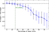 |
Fig. A.1. Difference between the true slope chosen to build the mock sample and the one recovered with the fit procedure. Each point shows the mean and standard deviation obtained from 250 mock samples created with a given percentage of upper limits. The upper limit percentage in the BASS sample is 16%, and we expect our fitting method to still be able to determine the correct slope. |
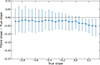 |
Fig. A.2. Difference between the true slope chosen to build the mock sample and the one recovered with the fit procedure, assuming 15% fraction of upper limits, and varying the value of the true slope. Each point shows the mean and standard deviation obtained from 250 mock samples created with a given slope. |
Appendix B: Adding FWHM
In La Franca et al. (2014), the authors reduced the dispersion in the relation between the excess variance and the luminosity by including the measurements of the FWHM of broad lines. The reasoning starts from the assumption that the primary driver of the observed relation is the MBH, with the luminosity following as a secondary effect, given its dependence on the mass itself. If this is indeed the case, it is possible to combine the variance-mass and mass-luminosity relations to derive
![Mathematical equation: $$ \begin{aligned} \log (\sigma ^2) = \alpha [\log (L) + 4 \log (\mathrm{FWHM} )] + \gamma . \end{aligned} $$](/articles/aa/full_html/2026/06/aa58009-25/aa58009-25-eq25.gif) (B.1)
(B.1)
By calibrating this relation, one can estimate an AGN’s intrinsic luminosity from its X-ray excess variance and broad-line FWHM. This, in turn, allows its distance to be determined. La Franca et al. (2014) incorporated FWHM from Hβ and Paβ into their analysis, observing significant reductions in the observed dispersion with respect to the case of luminosity alone versus luminosity and FWHM together. In particular, they found: from 1.78 to 1.12 dex for the L5100 Å-Hβ combination, from 1.36 to 1.06 dex for the L2 − 10 keV-Hβ combination, and from 1.33 to 0.71 dex for the L2 − 20 keV-Paβ combination. However, their sample sizes were relatively small, comprising 31, 38, and 18 objects, respectively, for the three combinations.
In the present work, we do not observe a smaller dispersion when fitting the excess variance against black hole mass than against luminosity. Therefore, we do not expect the inclusion of the FWHM to change the observed dispersion. Still, for completeness and to compare with the results in La Franca et al. (2014), we performed the analysis presented here. Our dataset includes 88 objects with Hβ measurements, more than double the sample size used by La Franca et al. (2014), and 49 objects with Paβ measurements, nearly triple their sample size. Additionally, we test this method with Hα and Paα, for which we have 115 and 39 objects, respectively. To test Eq. 8, we analysed different combinations of monochromatic luminosities and FWHM. For each of the four broad emission lines tested, we used the X-ray luminosity in the 2–10 keV band as the luminosity variable. Additionally, for Hβ, we tested the monochromatic luminosity at 5100 Å, while for Hα, we tested the luminosity at 6200 Å. Our goal was to test these optical/UV luminosities close to the broad lines as they may correlate more tightly with MBH in the context of the virial equation. Results are shown in Table B.1 and in Figs. C.1-C.5.
Fitting results for the relation log(σ2) vs luminosities and the FWHM with the slope β set to four
We compared our results for the 2–10 keV luminosity with the baseline total dispersion (δtot = 0.73 dex) and intrinsic dispersion (δint = 0.70 dex) obtained previously. Using Hα or Hβ as the FWHM indicator, we observed a slight improvement, with δtot reducing to 0.72 dex and δint remaining the same (for Hα) or decreasing slightly (for Hβ). Thus, the inclusion of Hα or Hβ has a limited impact. We also tested whether replacing the X-ray luminosity with the optical monochromatic luminosities at 5100 Å (Hβ) and 6200 Å (Hα) could further reduce the dispersion. However, as shown in Table B.1, this approach resulted in higher dispersion values (see also the figures in Appendix D). While monochromatic luminosities near the emission line should, theoretically, better trace the MBH in the virial equation, the stronger correlation between X-ray luminosity and excess variance may be more significant in practice. This could be attributed to the fact that X-ray and optical/UV observations are not simultaneous. Indeed, La Franca et al. (2014) also found smaller dispersion values when using X-ray luminosities rather than optical ones. When analysing the Paschen lines, we observed a more substantial reduction in dispersion. For Paα and Paβ, the total dispersion was reduced to δtot = 0.69 and 0.70 dex, respectively, with intrinsic dispersions of δint = 0.63 and 0.64 dex. These tighter relations are notable, despite the smaller sample sizes for the Paschen lines. Compared to La Franca et al. (2014), we observed lower dispersion values for all combinations of luminosities and lines common to that study. Doubling or tripling the sample size in our analysis appears to significantly improve the results, suggesting that further increases could yield even tighter correlations. However, contrary to La Franca et al. (2014), we do not observe a significant reduction in dispersion when using Hβ or Hα.
Our analysis assumes that the virial factor f in the virial equation is constant. However, this is a simplification, as the virial factor likely varies across objects due to differences in the geometry and kinematics of the BLR. Recently, the direct modelling of the BLR emission in RM campaigns has been proposed as a way to directly measure the virial factor f for single sources. However, such analyses are time-consuming and require a very high S/N to be performed (Villafaña et al. 2024). Indeed, only ∼40 AGNs have undergone such modelling (Villafaña et al. 2023). Still, even if we cannot directly measure f for all the objects in our sample, we can explore the effect of the dependence of the virial factor on other observable quantities. We tested whether the virial factor f depends on the FWHM of broad lines, as suggested by previous studies. A dependence of f ∝ FWHM−1 has been suggested (e.g. Mejía-Restrepo et al. 2018; Yu et al. 2019), based on the inclination dependence of the BLR. If this dependence holds, the slope associated with the FWHM term in Eq. B.1 would change from four to two. Using this relation, we repeated our analysis, with the results presented in Table B.2. For the Hβ and Hα lines combined with L2 − 10 keV, we observed reduced dispersions compared to not including the FWHM term. The improvement was even more pronounced for the Paschen lines, with the combination of Paα and L2 − 10 keV achieving the lowest intrinsic dispersion, δint = 0.58 dex. We also tested different values for the dependence of f on the FWHM, with f∼FWHM−η with η in the range from 0 to 2, and we still found that values around η∼1 provide the smallest observed dispersion. These results suggest that the virial factor may indeed depend on the FWHM, potentially due to inclination effects. Incorporating BLR modelling and objects with RM data could provide a more robust sample for calibration. However, RM samples may still be biased, as they often include AGNs with smaller MBH, which exhibit stronger variability, making monitoring campaigns more feasible. Addressing these biases and incorporating inclination effects into the analysis represent directions for future work.
Fitting results for the relation log(σ2) vs luminosities and the FWHM with the slope β set to two.
Appendix C: Excess variance versus X-ray Eddington ratio
We tested whether the short-timescale X-ray excess variance correlates with the X-ray Eddington ratio, 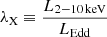 ,
,  . We fit a log-linear relation of the form log(σNXS2) = a log(λX)+b, using the iterative procedure described in Sect. 3, and we report results for both the full sample and the RM-only subsample. For the full sample we find a weak positive slope aall = +0.31 ± 0.15, which differs from zero at the ∼2.1σ level. For the RM-only subsample the slope is aRM = +0.35 ± 0.41, fully consistent with no correlation. The corresponding fits and 1σ confidence bands are shown in Fig. C.1 left and right panels. Interpreting σNXS2 versus λX is non-trivial because log LEdd is effectively proportional to log MBH, and LX and MBH are themselves strongly correlated in our sample. Consequently, λX introduces covariance between variables already entering the σ2–MBH and σ2–LX relations, making the slope sensitive to that. Given these caveats and the marginal significance, we refrain from drawing a physical conclusion from the weak positive trend. In the main text (Sect. 4.4), we therefore adopt the analysis based on bolometric Eddington ratios derived from SED fitting.
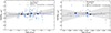 |
Fig. C.1. Relation between the X-ray excess variance and the X-ray Eddington ratio, λX ≡ L2 − 10 keV/LEdd. Left: Full sample. Right: RM-only subsample. Cyan points show detections; red triangles show upper limits. Dark-blue stars indicate medians in λX bins (shown for visualisation only). The dashed black lines show the best-fit relations; the grey shaded areas show the 1σ confidence intervals. Slopes and intercepts are indicated in each panel. |
Appendix D: Additional figures
Here we provide the plots for the fit of log σNXS2 = αlog(L)+βFWHM + γ, when using the monochromatic luminosity at 5100Å and 6200Å when fitting using the FWHM of the Hβ and Hα lines, respectively. On one hand, using a monochromatic continuum closer to the emitted line should be a more accurate choice for the virial equation for the BH mass measurement. However, we observe a worse overall performance in terms of observed dispersion when using optical monochromatic continuum luminosities compared to 2-10 keV monochromatic luminosities. This could be because, as the X-ray and optical observations are not simultaneous, the X-ray luminosity is a better proxy as it more strongly correlates with the X-ray excess variance.
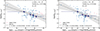 |
Fig. D.1. Relation between the X-ray excess variance and the combination of monochromatic luminosity and broad line FWHM for the Hβ line, σNXS2 = α(log(L)+βFWHM)+γ. N = 87; the legend is the same as the previous figures. Left: L is the 2-10 keV luminosity, b = 4, as predicted from the virial equation. Right: L is the 2-10 keV luminosity, b = 2. When b = 2, we observed a lower value of the dispersion. |
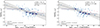 |
Fig. D.2. Same as Fig. D.1 but for the Hα broad line. N = 114. Again, we see that the dispersion slightly lowers going from b = 4 to b = 2. |
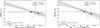 |
Fig. D.3. Same as Fig. D.1 but using the Paα broad line FWHM. N = 40. We observe a reduction in dispersion when going from b = 4 to b = 2. |
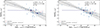 |
Fig. D.4. Same as Fig. D.1 but using the Paβ broad line FWHM. N = 56. We observe a reduction in dispersion when going from b = 4 to b = 2. |
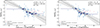 |
Fig. D.5. Same as Fig. D.1 but for the Hα broad line, using the 6200 Å monochromatic luminosity. N = 114. |
Appendix E: Additional cosmological plots
In Sect. 6 we performed the simulation considering the objects that would have X-ray observations with AXIS and/or NewAthena, and a spectroscopic redshift value obtained using Euclid. It could be that a redshift estimate would be obtained with other probes. In this appendix we show the Hubble diagram for the ’best case scenario’ in which all objects with an X-ray excess variance measurement obtained by AXIS and/or NewAthena would have a spectroscopic redshift. In particular, the right panel in Fig. D.1 shows how with the deep surveys planned for NewAthena we would be able to reach up to redshift ∼5, testing the expansion rate of the Universe when it was less than a billion years old.
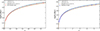 |
Fig. E.1. Left: Simulated Hubble diagrams obtained by using the relation between X-ray excess variance and 2-10 keV luminosity to derive the luminosity distance DL. The diagram is generated for a sample of objects expected to be observed by AXIS, assuming they will all have a spectroscopic redshift measurement. Right: Same simulation but for the NewAthena telescope. |
All Tables
Fitting results for the relation log(σ2) vs luminosities and the FWHM with the slope β set to four
Fitting results for the relation log(σ2) vs luminosities and the FWHM with the slope β set to two.
All Figures
|
Fig. 1. Left: Relation between the 2–10 keV excess variance (σNXS2) (obtained with time bins of 100 s) and the black hole mass (MBH) for the sample of 134 objects. Filled cyan circles show full detections; red down-pointing triangles show upper limits; the grey shaded area shows the confidence interval at 1σ for the best-fit log-linear relation. Blue stars represent the median value of the MBH and the excess variance in six MBH bins, chosen so that in each bin there are at least 20 objects. Blue error bars indicate the bin width. Blue stars are placed solely to guide the eye, as the fit is performed on the entire sample. The p-value of the relation and the total scatter δtot are displayed, together with the best fit result. The best fit is reported on the plot as |
| In the text | |
|
Fig. 2. Relation between the 2–10 keV excess variance (obtained with time bins of 100 s) and different monochromatic luminosities. The legend is the same as in Fig. 1. Top: Relation obtained using the 2–10 keV monochromatic luminosity. Middle: Relation obtained using the 5100 Å monochromatic luminosity. Bottom: Relation obtained using the 6200 Å monochromatic luminosity. Sample size N = 134. |
| In the text | |
|
Fig. 3. Residual analysis to assess whether black hole mass or luminosity more fundamentally drives X-ray excess variance. Upper left: Residuals from the best fit of the log(σ2)–log(L2 − 10 keV) relation plotted against log(MBH). A weak trend can be observed (α = −0.10 ± 0.06), but the obtained p-value is 0.88, against the significance of the trend. Upper right: Residuals from the log(σ2)–log(MBH) relation plotted against log(L2 − 10 keV). There is no significant trend (α = −0.06 ± 0.08), and the p-value is 0.75. These findings suggest that for this dataset, neither MBH nor L can be considered the ‘main driver’ of the variability against the other. Lower left: Same as in the upper-left panel but restricted to the RM-only sample. A 2.3σ significant negative dependence on MBH is observed. Lower right: Same as in the upper-right panel but restricted to the RM-only sample. A 2σ positive dependence on luminosity is observed. This marginally suggests that MBH is more predictive than the luminosity. |
| In the text | |
|
Fig. 4. Relation between the X-ray excess variance σNXS and the λEdd. Blue stars represent averaged bins in the Eddington ratio and are shown to guide the eye. Left: Fit performed for the whole sample, where 102 objects out of 134 have black hole masses estimated using the virial equation and 32 have RM estimates. Despite the reduced fraction of upper limits and increased precision of the λEdd estimates compared with other studies, there is still no significant relation between X-ray variability and the λEdd. Right: Same analysis for the subsample of objects with black hole masses derived from RM (N = 32). There is an anti-correlation, but it is only slightly significant. |
| In the text | |
|
Fig. 5. Proof-of-concept Hubble diagram for the BASS sample (grey points) using the relation between X-ray excess variance and the 2–10 keV luminosity. The dark orange points show the mean values obtained by binning the sample into nine equal-sized bins. Cyan points represent the Pantheon+ Supernovae Ia sample (Scolnic et al. 2018), while the black line represents the prediction from a standard flat ΛCDM model. The redshift range and limited statistics of the BASS sample currently undermine the cosmological implementation of the method, but future probes might open new possibilities (see Sect. 6). |
| In the text | |
|
Fig. 6. Left: Simulated Hubble diagram obtained using the relation between X-ray excess variance and 2–10 keV luminosity to derive the luminosity distance, DL, for sources expected to be observed by AXIS (to measure variability) and Euclid (to provide spectroscopic redshifts). Right: Same simulation but for NewAthena, considering its planned deep survey coverage. The light cyan points represent the luminosity distances obtained from SNe Ia in the Pantheon+ sample. The solid, dashed, and dot–dashed black curves correspond to different cosmological models, which overlap at low redshift but diverge at z ≳ 2, where AGNs become valuable standardisable candles. |
| In the text | |
|
Fig. A.1. Difference between the true slope chosen to build the mock sample and the one recovered with the fit procedure. Each point shows the mean and standard deviation obtained from 250 mock samples created with a given percentage of upper limits. The upper limit percentage in the BASS sample is 16%, and we expect our fitting method to still be able to determine the correct slope. |
| In the text | |
|
Fig. A.2. Difference between the true slope chosen to build the mock sample and the one recovered with the fit procedure, assuming 15% fraction of upper limits, and varying the value of the true slope. Each point shows the mean and standard deviation obtained from 250 mock samples created with a given slope. |
| In the text | |
|
Fig. C.1. Relation between the X-ray excess variance and the X-ray Eddington ratio, λX ≡ L2 − 10 keV/LEdd. Left: Full sample. Right: RM-only subsample. Cyan points show detections; red triangles show upper limits. Dark-blue stars indicate medians in λX bins (shown for visualisation only). The dashed black lines show the best-fit relations; the grey shaded areas show the 1σ confidence intervals. Slopes and intercepts are indicated in each panel. |
| In the text | |
|
Fig. D.1. Relation between the X-ray excess variance and the combination of monochromatic luminosity and broad line FWHM for the Hβ line, σNXS2 = α(log(L)+βFWHM)+γ. N = 87; the legend is the same as the previous figures. Left: L is the 2-10 keV luminosity, b = 4, as predicted from the virial equation. Right: L is the 2-10 keV luminosity, b = 2. When b = 2, we observed a lower value of the dispersion. |
| In the text | |
|
Fig. D.2. Same as Fig. D.1 but for the Hα broad line. N = 114. Again, we see that the dispersion slightly lowers going from b = 4 to b = 2. |
| In the text | |
|
Fig. D.3. Same as Fig. D.1 but using the Paα broad line FWHM. N = 40. We observe a reduction in dispersion when going from b = 4 to b = 2. |
| In the text | |
|
Fig. D.4. Same as Fig. D.1 but using the Paβ broad line FWHM. N = 56. We observe a reduction in dispersion when going from b = 4 to b = 2. |
| In the text | |
|
Fig. D.5. Same as Fig. D.1 but for the Hα broad line, using the 6200 Å monochromatic luminosity. N = 114. |
| In the text | |
|
Fig. E.1. Left: Simulated Hubble diagrams obtained by using the relation between X-ray excess variance and 2-10 keV luminosity to derive the luminosity distance DL. The diagram is generated for a sample of objects expected to be observed by AXIS, assuming they will all have a spectroscopic redshift measurement. Right: Same simulation but for the NewAthena telescope. |
| In the text | |
Current usage metrics show cumulative count of Article Views (full-text article views including HTML views, PDF and ePub downloads, according to the available data) and Abstracts Views on Vision4Press platform.
Data correspond to usage on the plateform after 2015. The current usage metrics is available 48-96 hours after online publication and is updated daily on week days.
Initial download of the metrics may take a while.