


| Issue |
A&A
Volume 710, June 2026
|
|
|---|---|---|
| Article Number | A40 | |
| Number of page(s) | 21 | |
| Section | Cosmology (including clusters of galaxies) | |
| DOI | https://doi.org/10.1051/0004-6361/202556431 | |
| Published online | 29 May 2026 | |
CHEX-MATE: Cluster multi-probes in three dimensions (CLUMP-3D)
II. Combined gas and dark matter analysis from X-ray, SZE, and WL
1
California Institute of Technology, 1200 E. California Blvd., MC 367-17 Pasadena, CA 91125, USA
2
Korea Advanced Institute of Science and Technology (KAIST), 291 Daehak-ro, Yuseong-gu, Daejeon 34141, Republic of Korea
3
INAF – Osservatorio di Astrofisica e Scienza dello Spazio di Bologna, Via Piero Gobetti 93/3, I-40129 Bologna, Italy
4
INFN, Sezione di Bologna, viale Berti Pichat 6/2, I-40127 Bologna, Italy
5
Université Paris Saclay, IRFU/CEA, 91191 Gif-sur-Yvette, France
6
Department of Astronomy, University of Geneva, Ch. d’Ecogia 16, CH-1290 Versoix, Switzerland
7
Academia Sinica Institute of Astronomy and Astrophysics (ASIAA), No. 1, Section 4, Roosevelt Road, Taipei 106216, Taiwan
8
Dipartimento di Fisica, Università degli studi di Roma Tor Vergata, Via della Ricerca Scientifica 1, I-00133 Roma, Italy
9
INFN, Sezione di Roma ‘Tor Vergata’, Via della Ricerca Scientifica, 1, 00133 Roma, Italy
10
Department of Physics, Informatics and Mathematics, University of Modena and Reggio Emilia, 41125 Modena, Italy
11
Laboratoire d’Astrophysique de Marseille, Aix-Marseille Univ., CNRS, CNES, 13013 Marseille, France
12
Institut d’Astrophysique de Paris, UMR7095 CNRS & Sorbonne Université, 98bis Bd Arago, 75014 Paris, France
13
Jodrell Bank Centre for Astrophysics, Department of Physics and Astronomy, The University of Manchester, Manchester, M13 9PL, UK
14
INAF, Istituto di Astrofisica Spaziale e Fisica Cosmica di Milano, Via A. Corti 12, 20133 Milano, Italy
15
Center for Astrophysics | Harvard & Smithsonian, 60 Garden Street, Cambridge, MA 02138, USA
16
INAF – Osservatorio Astronomico di Trieste, Via Tiepolo 11, I-34131 Trieste, Italy
17
Department of Physics; University of Michigan, Ann Arbor, MI 48109, USA
★ Corresponding author: This email address is being protected from spambots. You need JavaScript enabled to view it.
Received:
15
July
2025
Accepted:
16
March
2026
Abstract
Under the standard model of hierarchical structure formation, the overall geometry of galaxy clusters is better described by a triaxial ellipse than by a sphere. As a result, the application of spherically symmetric models can result in significant biases, with masses derived from weak-lensing observations being particularly sensitive. These biases can be mitigated by fitting a triaxial model, but this requires deep multi-probe data along with a set of physically motivated models to describe them. We present a multi-probe triaxial analysis method based on the data available for galaxy clusters in the Cluster Heritage project with XMM-Newton – Mass Assembly and Thermodynamics at Endpoint of structure formation (CHEX-MATE), which includes X-ray data from XMM-Newton, Sunyaev-Zel’dovich effect maps from Planck and ACT, and weak-lensing data from Subaru. This work builds upon our previous development of a gas-only X-ray and Sunyaev-Zel’dovich triaxial fitting formalism in Paper I. After verifying our approach using mock observations of model clusters with known properties, we applied it to the CHEX-MATE galaxy cluster PSZ2 G313.33+61.13 (Abell 1689). We found that the cluster is elongated along the line of sight relative to the plane of sky by a factor of ℛLP = 1.20 ± 0.04. As a result, the weak-lensing mass obtained from our triaxial fit, M200c = (13.88+1.73−1.43) × 1014 M⊙, is significantly lower than the value of (17.77+2.00−1.75) × 1014 M⊙ obtained from a spherically symmetric fit that otherwise employed the same method. Our triaxial fit finds a concentration of c200c = 8.66+2.08−1.70, consistent with the spherically symmetric value of 9.99+2.26−1.8, which suggests that the unexpectedly high concentration in Abell 1689 is not due to triaxiality and orientation. We also measured the nonthermal pressure fraction at radii between 0.18–1.37 Mpc and found a minimum of approximately 20% at intermediate radii, increasing to near 30% at the smallest and largest radii, and with a typical measurement precision of ±5%.
Key words: gravitational lensing: weak / galaxies: clusters: general / galaxies: clusters: intracluster medium / galaxies: clusters: individual: Abell 1689 / cosmology: observations / X-rays: galaxies: clusters
© The Authors 2026
 Open Access article, published by EDP Sciences, under the terms of the Creative Commons Attribution License (https://creativecommons.org/licenses/by/4.0), which permits unrestricted use, distribution, and reproduction in any medium, provided the original work is properly cited.
This article is published in open access under the Subscribe to Open model. This email address is being protected from spambots. You need JavaScript enabled to view it. to support open access publication.
1. Introduction
Within the current standard cosmological framework, structure formation proceeds as a hierarchical merging process (Davis et al. 1985; Kravtsov & Borgani 2012), with galaxy clusters forming from the gravitational collapse of the most dense peaks in the initial primordial density field (Kaiser 1986, 1991). Anisotropic collapse results in a web of filaments that connect galaxy clusters and other large objects and continue to feed their growth (Bond et al. 1996). Within this geometry, the primary nodes of the web (i.e., clusters) are better described by triaxial ellipses than by spheres (Limousin et al. 2013; Despali et al. 2014; Bonamigo et al. 2015), with numerical simulations predicting preferential alignment between the elongated axes and the large-scale connected filaments (Frenk et al. 1988; Dubinski & Carlberg 1991; Warren et al. 1992; Cole & Lacey 1996; Jing & Suto 2002; Hopkins et al. 2005; Bailin & Steinmetz 2005; Kasun & Evrard 2005; Paz et al. 2006; Allgood et al. 2006; Bett et al. 2007; Muñoz-Cuartas et al. 2011; Gao et al. 2012).
A range of observational evidence demonstrated that clusters are elliptical in the two-dimensional plane of sky (POS). In particular, the projected signals from various probes, such as the X-ray surface brightness (SB, Lau et al. 2012), the Sunyaev-Zel’dovich (SZ) effect scattering of cosmic microwave background photons (Sayers et al. 2011), and strong and weak gravitational lensing (SL and WL, Oguri et al. 2010) generally both display some degree of elongation in the POS. While clusters have long been known to deviate from spherical symmetry, limitations in data quality and availability have often resulted in modeling them as spherical objects, particularly for SZ (e.g., Bleem et al. 2024) and WL (e.g., Chiu et al. 2025) observations. Even with exquisite data, critical three-dimensional geometric information is lost because the observed signals are a two-dimensional projection, and this generally prevents analyses employing a single observational probe from fitting nonspherical models. To accurately recover the triaxial cluster morphology, deep multi-probe observational data must be combined (e.g., Limousin et al. 2013).
For example, the three-dimensional properties of a cluster can be inferred from the combination of X-ray and SZ data by using their respective dependences on the gas density and temperature of the intracluster medium (ICM). These data redundantly probe ICM thermodynamics, but with different weighting for the line-of-sight (LOS) projection of the observed signals. The X-ray emission primarily stems from thermal Bremsstrahlung (Sarazin 1986), with
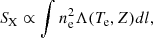
where ne is the electron density, and Λ(Te, Z) is the cooling function, which depends on temperature (Te) and metallicity (Z). For typical ICM temperatures and metallicities, Λ(Te, Z) is approximately constant for soft-band measurements of SX at ≲2 keV (Ettori 2000). In contrast, the SZ signal brightness (Sunyaev & Zeldovich 1972) is given by
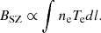
Spectroscopic fits to X-ray observations can also measure the ICM temperature, Tsp, and in the limit of an isothermal and isodensity gas distribution along the LOS, the extent of the cluster along the LOS, Δl, can therefore be obtained by combining these three measurements as
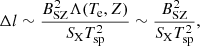
where the right-hand expression is approximately valid for SX measured in the soft band. In practice, deviations from isothermality and isodensity prevent such a simplistic calculation, but information on the LOS extent of the cluster can still be obtained from jointly modeling the X-ray and SZ data by using elliptically symmetric parametric models to describe the spatial variations in these thermodynamic quantities. An early analysis based on this approach was performed by De Filippis et al. (2005), who found that the spherical hypothesis was strongly rejected for the majority of objects in a sample of 25 clusters. In a later study considering the same data, Sereno et al. (2006) found a mixed population of prolate and oblate morphologies, with prolate shapes preferred among 60–76% of the sample. Subsequent triaxial analyses based on this general technique all found measurable deviations from spherical symmetry (e.g., Morandi et al. 2011; Morandi & Limousin 2012; Morandi et al. 2012; Sereno et al. 2017, 2018; Kim et al. 2024)
Alternatively, SL and WL datasets can be combined to make deprojected surface density maps and to then determine the triaxial structure of the cluster from them. This method typically assumes a Navarro-Frenk and White (NFW, Navarro et al. 1997) density profile in an elliptical coordinate basis. The projected NFW profile can be described in terms of the strength of the lens and the projected length scale, which is a function of cluster shape and orientation, and is fit to the observed lensing signals (i.e., shear, convergence, and magnification). This approach was applied to single clusters (e.g., Sereno & Umetsu 2011; Umetsu et al. 2012, who find mildly triaxial halos) and to an analysis of 20 clusters from the Custer Lensing And Supernovae survey with Hubble (CLASH, Postman et al. 2012) sample, with Chiu et al. (2018) finding a preference for prolate geometry that agrees well with the results from the joint X-ray and SZ analyses detailed above.
This work builds upon the triaxial fitting pipeline described in Kim et al. (2024, hereafter K24), which is based on the combination of SZ and X-ray data to obtain triaxial geometry by adding a WL analysis to their gas-only approach while additionally building on the WL fitting method described in Sereno et al. (2017). This expansion of the pipeline allows for a measurement of the total cluster mass. In more detail, K24 performed a joint X-ray and SZ analysis to constrain the geometrical properties of a cluster, which included two axial ratios that gave the relative lengths of the three orthogonal primary axes of a triaxial ellipse, along with their orientation relative to the LOS and POS. Sereno et al. (2017) included a total mass profile in their model that was constrained by the combination of SL and WL. They assumed constant axial ratios for this profile, which are different from the gas axial ratios, but are coaligned. As detailed below in Section 2.2, we instead only used WL data and assumed constant axial ratios for the gravitational potential, which are equal to the axis ratios of the gas distribution. This decision was motivated by the potential being smoother than the total mass profile (Stapelberg et al. 2022).
As a particular motivation to add WL to the model of K24, we note that the three-dimensional ellipticity of clusters, combined with orientation, is the primary cause of bias in single-cluster mass measurements from WL (e.g., Meneghetti et al. 2010b; Euclid Collaboration: Giocoli et al. 2024). This is due to the especially strong degeneracy between the total mass and elongation along the LOS, and fitting a three-dimensional elliptical model allowed us to eliminate most of this bias. In addition, cluster orientation can affect the inferred shape of the radial profile of mass density, which is often quantified by a mass-dependent concentration in the context of the NFW model. Previous studies have shown that exceptionally high concentrations found for individual clusters were a result of elongation (Broadhurst et al. 2008; Oguri et al. 2009; Sereno et al. 2010; Meneghetti et al. 2014). Thus, a WL analysis that includes three-dimensional shape information provided by the gas observables offers the promise of minimally biased individual cluster mass and concentration measurements.
These relatively unbiased mass reconstructions also open the possibility to probe the level of support against gravitational collapse due to motions outside of hydrostatic equilibrium (HSE) in the ICM, often referred to as nonthermal pressure (Pnt). There are various contributions to Pnt in the central and outer regions of the cluster. In the cluster core, feedback from a centrally located active galactic nucleus (AGN) is likely the primary heating source (McNamara et al. 2005). This heating is dynamic, as AGN jets inflate bubbles in the gas and transfer energy via multiple mechanisms, such as shocks, cavity heating, and convective mixing. Additionally, turbulence is driven on smaller scales by core sloshing from cluster merger events, dynamical friction, and galaxy motions (Khatri & Gaspari 2016; Gaspari et al. 2020; Romero et al. 2025). Direct measurements of the velocity structure in this region are enabled by X-ray spectroscopy from instruments such as the X-Ray Imaging and Spectroscopy Mission (XRISM, Tashiro et al. 2025). To date, XRISM has mainly focused on probing the region within the central ∼100 kpc in radius, extending beyond this region in one case. It typically found very low nonthermal pressure fractions (Pnt/Ptot ∼ 2 − 3%, XRISM Collaboration 2025a,b,c,d). These results are lower in general than those found from hydrodynamical simulations of clusters. However, accurately simulating the centrally located AGN is an active research area, and it is therefore unclear whether these XRISM measurements contradict the predicted values near 10% found in these simulations (Nelson et al. 2014; Angelinelli et al. 2020).
We focus on accurately reconstructing the distribution of gas and total mass, along with the thermodynamic properties of the gas, to obtain a measurement of Pnt in the outer cluster regions beyond 1 Mpc in radius. Numerical simulations suggest that clusters progressively deviate more from HSE with increasing radius well beyond R200c (∼2–3 Mpc) because of the newly accreted material that has not fully thermalized (Piffaretti & Valdarnini 2008; Lau et al. 2009; Nelson et al. 2014; Angelinelli et al. 2020). The in-falling material in this region is brought into thermal equilibrium with the ICM primarily through a series of radial shocks (Miniati et al. 2000), and the overall thermalization efficiency of these shocks can be quantified by the ratio of Pnt to the total pressure (Ptot). We note that Pnt includes turbulent and coherent motions. Modeling Pnt in simulations of cluster outskirts can be challenging due to resolution effects related to the low particle density in these regions, and it is therefore currently unclear whether they fully trace the relevant physics. Simulations generally agree that Pnt/Ptot are expected to increase with radius, but the predicted values of Pnt/Ptot near R200c span a wide range from approximately 15–40% (Nelson et al. 2014; Shi & Komatsu 2014; Shi et al. 2015; Vazza et al. 2018; Eckert et al. 2019; Pearce et al. 2020; Angelinelli et al. 2020; Sayers et al. 2021). Observational studies of the ensemble average value of Pnt/Ptot from modest samples of ≃10 clusters also span a wide range, but have generally found lower values, with Pnt/Ptot ≃ 10 − 25% near R200c (Siegel et al. 2018; Eckert et al. 2019; Sarkar et al. 2025), potentially suggesting more efficient thermalization than typically found in the simulations.
We demonstrate our triaxial modeling pipeline with a multi-probe dataset assembled as part of the Cluster HEritage project with XMM-Newton: Mass Assembly and Thermodynamics at the Endpoint of Structure Formation collaboration1 (CHEXMATE; CHEX-MATE Collaboration 2021), including SZ, X-ray SB, and temperature, and WL shear measurements of the galaxy cluster PSZ2 G313.33+61.13 (hereafter Abell 1689). The SZ and X-ray portion of the analysis largely follows that detailed in K24. We mainly focus on the integration of a WL analysis into the established gas-only analysis and on the subsequent mass profile and nonthermal pressure measurements obtained from this updated pipeline. In Section 2 we summarize the triaxial analysis method, including our modeling formalism. In Section 3 we describe the calculation performed to obtain a radial profile of the nonthermal pressure support from our triaxial fits. Section 4 reviews the results from running the fitting pipeline on a set of mock observations of known cluster models. This provides an understanding of potential biases introduced by the fit and demonstrates that we can accurately recover the known input parameters. We describe the observed dataset for Abell 1689 in Section 5 and the results of the fit to these data in Section 6. A comparison to other results in the literature is detailed in Section 7, including those obtained by Chappuis et al. (2025) using the same CHEX-MATE data, but a much different modeling formalism. Throughout this study, we adopt a ΛCDM cosmology characterized by H0 = 70 km s−1 Mpc−1, ΩM = 0.3, and ΩΛ = 0.7.
2. Triaxial analysis formalism
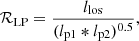
Our cluster model assumes a triaxial shape, and we followed the mathematical description of a triaxial cluster geometry developed in K24, of which we provide a brief description here. The intrinsic cluster geometry is connected to the properties observed in the POS by writing the thermodynamic profiles of the ICM and the gravitational potential as functions of ζ, the three-dimensional ellipsoidal radius, which is defined in the intrinsic coordinate system of the ellipsoid. Because the axes of these intrinsic coordinates may not align with those of the observer, we related the two using three Euler angles: θ, ϕ, and ψ. K24 defines the elongation of the ellipsoid, e∥, as the ratio of the llos, which is the half size along the observer LOS of the ellipse (i.e., its LOS extent) corresponding to the projection of the ellipsoid onto the plane that is perpendicular to the sky plane, and lp1, the semimajor axis of the ellipse corresponding to the projection of the ellipsoid on the POS. We used a different definition from K24, which we denote as ℛLP, and is given by
 (1)
(1)
where lp2 is the semiminor axis of the ellipse corresponding to the projection of the ellipsoid on the POS, so (lp1 * lp2)0.5 is then the effective spherical radius of the projected ellipse.
The three-dimensional distributions of the ICM and gravitational potential were projected and expressed as functions of ξ, the two-dimensional projected elliptical radius, via
 (2)
(2)
where xζ = ζ/ls, with ls being the major axis of the ellipsoid, xξ = ξ/lp1, and pi are the parameters describing the intrinsic three-dimensional (elliptical) radial profile. The projection integration for each of the observables can be computationally expensive, so to expedite the calculation, we created a linearly spaced sample of the (normalized) elliptical radius xξ and interpolated the integration results while generating a model. All the projections were performed numerically with sufficient sampling to ensure a fractional precision of approximately 10−3 (or better), far below measurement uncertainties of the observables.
For our application to Abell 1689 in this analysis, the observational data included two-dimensional images of the SZ Compton-y, X-ray SB, and the two-components of the WL reduced shear signal, as well as one-dimensional projected radial profiles of X-ray SB and temperature data. The triaxial model detailed in this section allows us to generate analogous images and radial profiles based on the model parameters in Table 1. The observed and model-generated data can be directly compared within our fitting pipeline to constrain the parameter values.
Model parameters and assumed priors.
2.1. ICM model
We obtained constraints on the thermodynamic quantities of the ICM through jointly modeling the SZ signal with the X-ray SB and temperature. To do this, we assumed three-dimensional profiles for the electron density ne(ζ), for which we used a Vikhlinin profile (Vikhlinin et al. 2006; Ettori et al. 2009), and electron pressure Pe(ζ), for which we use a generalized Navarro-Frenk-White (gNFW) profile (Navarro et al. 1997; Nagai et al. 2007; Arnaud et al. 2010). The free parameters of these profiles are listed in Table 1. A discussion regarding parameter degeneracies in Pe(ζ) is presented in Appendix B. These were connected to our two-dimensional observables via projection of the three-dimensional functions along the line of sight within a triaxial basis (Eq. (2)). The SZ Compton-y parameter is given by
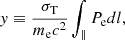 (3)
(3)
and the X-ray surface brightness of the ICM due to thermal Bremsstrahlung and line emission is given by
 (4)
(4)
where the electron temperature for the cooling function is calculated as
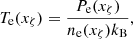 (5)
(5)
and we used a constant metallicity of 0.3 times the solar abundance. A grid of values for Λ(Te, Z) was precalculated using using the Python package pyproffit (Eckert et al. 2020), and this table is then interpolated over Te and Z when evaluating the model. The emissivity calculation takes into account the instrument response within the energy band [0.7–1.2] keV and the primordial helium fraction (He/H), equal to nH = 7.72 × 10⁻² for Abell 1689 (Bartalucci et al. 2023). Projected maps of ICM temperature were obtained via spectroscopic fits to the X-ray data. The spectroscopic temperature (Tsp) was approximated within our model based on the formalism of Mazzotta et al. (2004).
2.2. Gravitational potential model
The addition of a WL analysis enabled the modeling of the gravitational potential, and therefore, the cluster density profile. In general, the effect of WL by a matter distribution on a background source is characterized by convergence, κ, and shear, γ. The shear introduces a quadrupole anisotropy in the background images, which can be observed from ellipticities of background galaxies. The observable quantity for quadrupole WL is generally not γ, but the reduced gravitational shear (Umetsu 2020), defined as
 (6)
(6)
The reduced shear is connected to the underlying gravitational potential through the lensing potential, which is the rescaled projection of the three-dimensional Newtonian potential on the lens plane,
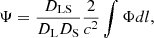 (7)
(7)
where DL, DS, and DLS are the angular diameter distances from the observer to the lens, which is the galaxy cluster in this case, the observer to the source, and the lens to the source, respectively. The shear is defined as a complex vector with spin-2 rotational symmetry γ = (γ1,iγ2), on the lens plane, and its components are calculated from the lensing potential as
 (8)
(8)
using the shorthand notation  . The convergence is
 (9)
(9)
The two components of the reduced shear can then be constructed from Eqs. (8) and (9), as defined in Eq. (6) through the projection of the gravitational potential in our triaxial model (Eq. (2)).
Rather than assuming the total density profile is elliptically symmetric within our triaxial basis, we assumed that the gravitational potential follows such a geometry. This decision is motivated in part by simulations, which suggest it is better to fit the potential because it is rounder and smoother than the total density (Stapelberg et al. 2022). In addition, it also allowed us to make the assumption that the isopotential surfaces follow the ICM isodensity surfaces, which is strictly true in the case of an idealized pressure distribution (Fox & Pen 2002) and found to be approximately true in numerical simulations of galaxy clusters (Lau et al. 2011). Thus, the triaxial ellipse describing the gravitational potential has an identical shape to the ICM (qpot = qICM), including co-alignment of the principal axes.
The gravitational potential can be determined from the total density by inverting Poisson’s equation,
 (10)
(10)
where ρ is the total density. This calculation was performed numerically, so any functional form for ρ is allowed. Because we assumed that the isopotential surfaces are elliptically symmetric with axial ratios that are constant with radius, surfaces of constant density will in general have axial ratios that vary with radius. Thus, it is not possible to describe ρ using an analytic form within this elliptical basis. So, we initially inverted Eq. (10) assuming a spherically symmetric ρ(r) based on
 (11)
(11)
We then evaluated this numerically tabulated function for Φ(r) on a three-dimensional elliptical grid, with the radial coordinate being ζ. This ensured that we obtain an elliptical gravitational potential Φ(ζ) that has identical axial ratios to those of the ICM. For this work, we assumed the initial spherically symmetric ρ(r) follows the NFW form with
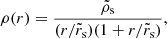 (12)
(12)
where  and
and  are the characteristic density and scale radius. We emphasize that Φ(ζ) is the quantity that is projected along the line of sight in Eq. (2) to obtain our WL observables.
It is common to quantify the total density distribution by M200c, which is the total mass within a sphere of radius R200c, and a concentration c200c = R200c/rs where rs denotes the radius where the logarithmic slope of the density profile is equal to −2. To obtain these quantities from our elliptical potential Φ(ζ) we proceeded as follows. The underlying density distribution in three-dimensions corresponding to Φ(ζ) was found by solving Poisson’s equation numerically in Cartesian coordinates as
 (13)
(13)
As noted above, the axial ratios corresponding to constant values of ρ(ζ) will in general vary with radius. To obtain M200c, we spherically integrated ρ(ζ) in three-dimensions. To determine c200c, we spherically averaged ρ(ζ) to calculate the scale radius rs as defined above. We note that  and
and  are distinct from the ρs and rs associated with this spherically averaged profile of ρ(ζ), from which we find M200c and c200c. Therefore,
  and
and  are not physically meaningful in this context, but are used here to connect M200c and c200c back to Eq. 10. For a given set of input parameters (qICM, 1, qICM, 2,
  and
and  ), we thus obtained unique values of the physical quantities of interest, M200c and c200c. Spanning the full set of allowed input parameter values, we then tabulated the relation between them and M200c and c200c. By interpolating this table, we could then connect any combination of M200c and c200c to the underlying values
  and
and  for a given qICM, 1 and qICM, 2. It is important to note that, although our formalism includes an NFW ρ(r) as a starting point, and we quantify the mass distribution via M200c and c200c, the underlying density distribution obtained from Eq. (13) does not strictly follow an NFW distribution.
2.3. Fitting formalism
The χ2 statistic was used to define the likelihood of the model. We used emcee (Foreman-Mackey et al. 2013), a Python-based affine-invariant ensemble Markov chain Monte Carlo (MCMC; Goodman & Weare 2010) package, for the model fitting process. The posterior distribution of the parameter values describing the triaxial model was constructed through MCMC sampling (Hogg & Foreman-Mackey 2018). We used the same definitions of χ2 for the SZ, X-ray SB and X-ray temperature data as in K24. We note that we updated the SZ covariance matrix calculation relative to K24 and detail this change in Appendix A. Additionally, we fit a radial profile of the X-ray temperature, rather than a two-dimensional map, as done in K24. This change is also detailed in Appendix A.
A dual approach employing two-dimensional and one-dimensional fits for the X-ray SB was used. We used two-dimensional data within the circular region that encloses 80% of the emission and a one-dimensional projected profile for the radial region outside of this, where the background and the source emission is comparable and signal-to-noise ratio is relatively low. A one-dimensional analysis in the exterior region is further motivated by a desire to mitigate biases in measuring X-ray SB caused by gas clumping, which can be achieved by taking the azimuthal median, rather than mean, of the observed data as suggested by Eckert et al. (2015). To generate one-dimensional X-ray SB profiles from the model, an azimuthal mean in annular bins was obtained from the two-dimensional projected model image in the exterior region. For the model, a mean averaging is approximately equivalent to median averaging, since the model is smooth and does not contain any clumps. We then used the combined likelihood from the two radial regions.
The χ2 function for the two-dimensional reduced shear is
![Mathematical equation: $$ \begin{aligned} \chi _{\mathrm{WL}}^2 = \sum _{i,j = 1}^{N_g} \sum _{\alpha ,\beta = 1}^2 \left[g_{\alpha ,i} - \hat{g}_{\alpha ,i}\right] \left(C_{\mathrm{WL}}^{-1}\right)_{\alpha \beta ,ij} \left[g_{\beta ,j} - \hat{g}_{\beta ,j}\right] , \end{aligned} $$](/articles/aa/full_html/2026/06/aa56431-25/aa56431-25-eq34.gif) (14)
(14)
where  is the model reduced shear map within a pixel, gi is the observed value, and CWL is the covariance matrix. In our error analysis we accounted for statistical noise (shape noise) and cosmic variance in the noise covariance matrix as CWL = Cstat + Clss. The shape noise was calculated according to Eq. 21 and Clss is the noise covariance due to uncorrelated large-scale structure (LSS) along the line of sight (Hoekstra 2003). The contribution from Cstat dominates over Clss, with the LSS noise amplitude being ∼1/100 of the shape noise amplitude, but the effect of cosmic noise is most important to include when the cluster signal itself is weak (Hoekstra 2003). This is the case for the large cluster radii we are interested in probing. The components of the Clss matrix were calculated following the prescription outlined in Kaiser (1992), Hu & White (2001), and Schneider et al. (2002). We used a lensing power spectrum Cϵϵ(l) calculated for a source population at zs = 1, using the cosmological parameters from the Wilkinson Microwave Anisotropy Probe (WMAP) Nine-Year results (Hinshaw et al. 2013).
The MCMC samples the total χ2, which is the sum of the χ2 of all three observational probes, within the parameter space near the best fit. To good approximation the three ICM observables constrain the parameters associated with the three-dimensional geometry. Given this geometry, the parameters of the total matter density are constrained entirely by the WL data and the parameters of the ICM density are primarily constrained by the X-ray SB. The combination of the SZ and X-ray temperature data then constrain the parameters of the ICM pressure.
2.4. Priors
For all the free model parameters except c200c, we applied uniform priors that are uninformative other than with regard to physical boundaries (e.g., qICM, 1 must take values between 0–1, see Table 1). It has been demonstrated that with WL alone, it is very difficult to simultaneously constrain M200c and c200c (e.g., Meneghetti et al. 2010a; Postman et al. 2012), and so it is common to place an informative prior on c200c, generally in the form of a δ-function or based on c − M relations obtained from simulations (e.g., Applegate et al. 2014; Euclid Collaboration: Giocoli et al. 2024; Hoekstra et al. 2015). We adopted the latter approach, employing a log-normal prior on c200c, with central value set by the average c − M relation given by the model of Diemer & Joyce (2019) and an assumed width based on the intrinsic scatter of this relation, corresponding to log(c200c)±0.16. This prior captures the expected intrinsic cluster-to-cluster scatter in c − M values in the Universe. To compute the central values of the c − M relation, we used the Python package colossus (Diemer 2018). For the span of the uniform prior we used for M200c, this c − M relation returns values for c200c between ∼4 − 6.5. This matches simulated concentrations from scale-free models and ΛCDM to an accuracy of 5% (Diemer & Joyce 2019).
3. Nonthermal pressure calculation
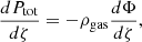
The addition of a WL analysis enables indirect measurement of the motions outside of thermal equilibrium that contribute to the total pressure of the cluster. From the constraints on the total mass density and the gas density profiles we can calculate the total pressure needed to offset gravitational collapse, Ptot, and the thermal component of pressure, Pth, in a three-dimensional triaxial basis. Because clusters are not in a state of perfect HSE, Ptot is in general greater than Pth and so the nonthermal component of pressure can be measured as the difference between Ptot and Pth under the assumption that the system is fully virialized. Within this formalism we are not sensitive to the underlying source of the nonthermal pressure support, which could be due to the combination of bulk motions, turbulence, magnetic fields, cosmic rays, or any other relevant terms. Assuming a state of generalized HSE, the total pressure is given by
 (15)
(15)
where Ptot = Pth + Pnt and ρgas is the gas density. Following the formalism of Fox & Pen (2002), for an elliptically symmetric system this reduces to
 (16)
(16)
and Ptot can be found by numerically integrating over the elliptical radius. We calculated ρgas from our assumed electron density profile (Section 2) through the relation
 (17)
(17)
where μe is mean molecular weight per free electron, taken to be equal to 1.14 as in Nagai et al. (2007), and mp is the mass of the proton. The Newtonian gravitational potential on a triaxial ellipsoid is calculated numerically as described in Section 2.2. The thermal pressure was calculated from the electron pressure through the relation
 (18)
(18)
where μ is mean molecular weight, taken to be equal to 0.59 as in Nagai et al. (2007). All of the above calculations were performed within a triaxial basis, and so we obtained a spherically averaged radial profile of Pnt by azimuthally averaging Ptot and Pth in three dimensions prior to computing their difference.
Because the above calculation is computationally expensive, it is not feasible to perform it within the fit at every step in the MCMC. So, the calculation was evaluated outside the fit, using the set of accepted samples from the MCMC. Because of this, it was not possible to apply a prior on Pnt to ensure its value remains in the physically allowed region ∈[0, Ptot]. For this analysis, we do not obtain values outside of this range, and so this lack of a prior does not present a problem for our fits. However, we note that techniques have been established for this exact scenario, as described in Sayers et al. (2021).
4. Demonstration with mock data
To validate the accuracy of our model fitting algorithm, we performed a full analysis using mock observations of galaxy clusters generated from our triaxial model using known input parameter values. The mock clusters have the same cluster redshift and source redshift as as Abell 1689, which are zcluster = 0.18 and zsource = 0.83. An extensive validation of the geometric and gas parameters was performed in K24, and so here we focus on validating our ability to constrain M200c, c200c, and the shape of the Pnt/Ptot profile. We ran three categories of tests: (A) Varying M200c and c200c with a common set of geometrical, electron density and gas pressure parameters (B) Varying the elongation with a common set of electron density, gas pressure, and total matter density parameters (C) Varying the shape of Pnt using unique sets of geometrical, electron density, gas pressure and total matter density parameters.
For a given set of parameters, we generated model SZ, X-ray SB and temperature maps, and WL shear maps following the modeling prescription outlined in Section 2. The SZ and X-ray model maps were convolved with the relevant instrument point spread functions (PSF) (See Section 5). Gaussian sampled noise from the error maps of the observational data for Abell 1689 was applied to each model map. An example set of mock observations that we used to test the pipeline is shown in Figure 1. We note that for this mock analysis we use two-dimensional data at all radii for each observable, since the model data are not prone to the same biases as the observed clusters. A corner plot with the recovered posteriors from a fit to the mock observations show in Figure 1, along with the input parameters used to generate the mocks, is given in Appendix C.
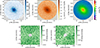 |
Fig. 1. Sample mock dataset generated from the smooth models outlined in Section 2. The SZ and X-ray observations were convolved with the Planck/ACT and XMM-Newton beams, respectively, and Gaussian sampled noise was applied to each map. The gray areas on the maps were excluded from the fits (see Section 5). |
Summary tables of the relevant recovered parameters from the fits to all the mock observations in each dataset are given in Appendix C. As expected, many of the input parameters fall within the 68% confidence intervals obtained from our fits, and are otherwise contained within the 90% confidence intervals. We show summary plots of the values of M200c and c200c obtained from fits to mock dataset A in Figure 2. In all cases, we found that the recovered values for M200c and c200c are consistent with the input values given the expected noise fluctuations and that there is no noticeable bias in the recovered c200c values due to the informative prior we apply.
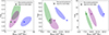 |
Fig. 2. Posterior distribution of M200c and c200c obtained from fits to mock observations. The shaded region for each posterior represents the 68% credible region. The cross indicate the input M200c and c200c used to generate the mock data. The shaded region that matches each cross in color corresponds to the posterior recovered from the mock data generated with that parameter pair. |
We calculated the corresponding radial profiles of Pnt/Ptot using the accepted samples from the fits to each dataset following the approach outlined in Section 3. A sample of results from each mock dataset is shown in Figure 3, with the first column corresponding the mock dataset A, the second column to mock dataset B, and the third column to mock dataset C. In most cases, the input profile of Pnt/Ptot fell within the 68% credible region of the recovered posterior over the full radial range, otherwise, it was contained within the 90% credible region. These results demonstrate that our pipeline can successfully recover mass, concentration, elongation, and Pnt for a variety of input parameter combinations and we infer that any potential bias in our fitting method is minimal compared to the measurement uncertainties.
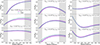 |
Fig. 3. Radial plots of the nonthermal pressure fraction (Pnt/Ptot) recovered from fits to mock observational data, generated with a range of M200cc200c and ℛLP values. The solid purple line represents the best fit model, and the shaded purple region is the corresponding 68% credible region calculated from the accepted MCMC samples. The dashed blue line is the nonthermal pressure fraction calculated from the input parameters used to generate the corresponding mock data. Shaded gray denotes regions where the mass distribution may not be fully constrained from the observed WL shear signal (see Section 5.2). |
5. Observational data
In this section, we summarize the SZ, X-ray, and WL data available for our analysis, which differ slightly from those used in K24, except for the two-dimensional X-ray SB map which is identical. These data were assembled as part of the CHEX-MATE project (CHEX-MATE Collaboration 2021). In particular for this analysis, we consider the CHEX-MATE galaxy cluster Abell 1689, which is at a redshift of z = 0.183. Abell 1689 is an extremely massive cluster, so it acts as a powerful gravitational lens and provides high quality lensing data. This makes it an ideal candidate for making precise mass measurements within our triaxial framework. Additionally, this cluster is well studied in the literature, allowing for detailed comparisons of these prior results with our primary measurements (mass, concentration, elongation, and nonthermal pressure content).
5.1. SZ and X-ray data
The two-dimensional X-ray SB map was produced from XMM-Newton observations using the Voronoi tessellation method (Cappellari & Copin 2003; Diehl & Statler 2006). The details of the image production are reported in Bartalucci et al. (2023) and Lovisari et al. (2024). Bright point sources in the X-ray SB map were masked and excluded from the analysis. This procedure was performed in a manner to ensure an approximately uniform residual cosmic X-ray background over the entire field of view, sufficiently low to not impact the fit (Ghirardini et al. 2019; Bartalucci et al. 2023). The two-dimensional X-ray SB used in this analysis is shown in the top middle of Figure 4.
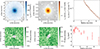 |
Fig. 4. SZ, X-ray, and WL data for the CHEX-MATE galaxy cluster PSZ2 G313.33+61.13 (Abell 1689). The ACT DR6 Compton-y map (top left), the X-ray SB map (top middle), X-ray SB radial profile (top right), two-component WL shear maps (bottom left and middle), and radial profile of X-ray temperature are shown. The grayed-out portions of the maps are data that were excluded from the fit. Bright point-like sources in the X-ray map are indicated by white circles. For the SZ and X-ray portion of the analysis, the data is limited to within the value of R500c obtained by Planck Collaboration XXVII (2016), equal to 7.42′ (1.37 Mpc). The X-ray SB employs a one-dimensional and two-dimensional approach. We use the two-dimensional data within the circular region that encloses 80% of the emission and one-dimensional data is used in the radial region outside of this. For the WL shear maps, we excluded data within 300 h−1 kpc comoving (∼360 kpc physical) to avoid regions containing SL features and significant contamination from cluster member galaxies. |
The one-dimensional projected radial profile of the X-ray SB used in this analysis was computed in a different manner than in K24. In brief, K24 calculated the azimuthal mean from the two-dimensional map, while we instead used the azimuthal median profile generated from the analysis of Bartalucci et al. (2023), which we summarize here. First, particle background subtracted Voronoi-binned X-ray SB maps with point sources masked were produced, ensuring 20 counts per bin on average. Concentric annuli centered on the X-ray peak were defined and the SB median profile was extracted by considering in each radial bin the median count rate of the Voronoi cells whose center lies within the annulus. In this way, the use of median profiles limits the bias caused by the emission of subclumps and substructures too faint to be identified and masked (e.g., Roncarelli et al. 2013; Zhuravleva et al. 2013). The sky background was estimated also using the median count rate. Then, the sky background subtracted profiles were re-binned to have at least nine counts per bin after background subtraction was performed on the particle background subtracted profiles. The portion of this radial profile used in this analysis is shown in the top right of Figure 4. More details regarding this change are given in Appendix A.
In this work, we chose to use the one-dimensional projected X-ray temperature profile, which differs from the approach of K24, who used a two-dimensional temperature map in their analysis. More details regarding this change are outlined in Appendix A. The technique to generate the projected temperature profiles is detailed in Rossetti et al. (2024), and we summarize it here. First, spectra in 15 concentric annuli around the X-ray peak were extracted, using the mos-spectra tool within the XMM-Newton Science Analysis System (SAS) and the Extended Source Analysis Software (ESAS, Snowden et al. 2008; Kuntz & Snowden 2008) embedded within SAS, which ensured a roughly constant signal-to-noise ratio in each radial bin. For each region, the corresponding redistribution matrix files (RMF) and ancillary response files (ARF) were extracted using the ESAS tool pn-spectra. A spectrum for the cosmic-ray induced particle background (CRPB) was then produced using the mos-back and pn-back tools. To calibrate the model of the sky background components, the spectrum obtained from an external annulus between 10.6′ and the edge of the field of view was used. The models of all the background components (quiescent particle background, cosmic X-ray background, Galactic halo, local hot bubble, and residual soft protons) are described in detail in Rossetti et al. (2024). For each region the spectra of the three detectors are jointly fit using XSPEC (Arnaud 1996), where the parameters of the background model are used as priors to derive the temperature, metal abundance and normalization of the ICM. The resulting temperature profile for Abell 1689 is shown in the bottom right panel in Figure 4, where the individual points in each radial bin are the mean of the posterior distribution of temperature values and the error bars are the corresponding 68% credible region.
We made use of a single SZ Compton-y map obtained from the combination of observations from the ground-based Atacama Cosmology Telescope (ACT) and Planck, which was generated by the ACT collaboration and is shown in the top left of Figure 4. In particular, we used the most recent version of this map, from ACT data release 6 (DR6, Coulton et al. 2024; Naess et al. 2025), which is deeper than the ACT-DR4 map used in by K24. The noise rms for the DR4 y-map is approximately 9 × 10⁻⁶, while for the DR6 y-map it is approximately 5 × 10⁻⁶ (for more details see Appendix A). We did not find any point-like sources, corresponding to either radio or dusty star-forming galaxies, within the region of the map used for our analysis, and thus no masking or subtraction of such sources was applied.
The X-ray and SZ data were restricted to within R500c obtained by Planck Collaboration XXVII (2016), equal to 7.42′ (1.37 Mpc), to mask out potential spurious signals at large radii that do not originate from Abell 1689. All the following results discussed in Section 6 are truncated at a radius of R500c for this reason.
5.2. Weak-lensing data
We performed a weak-lensing analysis of Abell 1689 using archival observations from the Subaru Suprime-Cam instrument. Full details of image reduction, photometry, and shape analysis for a sample comprising 40 CHEX-MATE clusters will be presented in forthcoming publications (Gavazzi et al.; Umetsu et al., in prep.). Our study is based on wide-field imaging in the B, V, RC, i+, and z+ bands, obtained with Suprime-Cam on the 8.2 m Subaru Telescope. Further details on the image processing and photometric redshift estimation for individual galaxies are given in Appendix F.
The reduced shear signal was measured from a background galaxy sample selected based on a color–color (CC) cut method. This method has been calibrated against evolutionary color tracks of galaxies and photo-z catalogs from deep multiwavelength surveys such as COSMOS (for details, see Medezinski et al. 2010, 2018). In our analysis, CC cuts were performed using BRCz+ photometry from Subaru/Suprime-Cam, which offers broad coverage across the optical wavelength range and is well-suited for cluster weak-lensing studies (e.g., Umetsu et al. 2014, 2022). These CC cuts yield a background sample of 16 428 galaxies, corresponding to a mean surface number density of ng ≈ 15 galaxies arcmin−2. For the selected background sample, we find a weighted mean of  Mpc−2 and
  .
.
Using the CC-selected sample of background galaxies, we computed the source-averaged reduced shear components, (g1(θn),g2(θn)), on a uniform grid of 48 × 48 pixels with Δθ = 0.5′ spacing, covering a 24′×24′ field centered on the X-ray cluster peak as
![Mathematical equation: $$ \begin{aligned} g(\boldsymbol{\theta }_n) = g_1(\boldsymbol{\theta }_n) + ig_2(\boldsymbol{\theta }_n) = \left[ \displaystyle \sum _{s\in n} { w}_{g (s)}g_{(s)} \right] \left[ \displaystyle \sum _{s\in n} { w}_{g(s)} \right]^{-1}, \end{aligned} $$](/articles/aa/full_html/2026/06/aa56431-25/aa56431-25-eq42.gif) (19)
(19)
where g(k) is an estimate of g(θ) for the sth galaxy at θ(s), and wg(s) is its statistical weight, wg(s) = 1/(σg(s)2 + σrms2). Here, σg(s) represents the measurement uncertainty for g(s), and σrms is the rms ellipticity for the background sample, which we take as σrms = 0.4 or equivalently,  per component (e.g., Umetsu et al. 2014). The resulting maps for g1 and g2 are shown in the bottom right and middle of Figure 4.
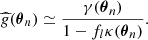
The source-averaged expectation (denoted by a hat symbol) for the observed g(θn) is given by (Seitz & Schneider 1997; Umetsu 2020)
 (20)
(20)
The error variance σg, n2 for gn is expressed as
![Mathematical equation: $$ \begin{aligned} \begin{aligned} \sigma ^2_{g,n}= \frac{ \sum _{s\in n} { w}_{g(s)}^2 \sigma ^2_{g(s)} }{ \left[ {\sum _{s\in n} { w}_{g(s)}} \right]^{2}}. \end{aligned} \end{aligned} $$](/articles/aa/full_html/2026/06/aa56431-25/aa56431-25-eq45.gif) (21)
(21)
We excised the center of the shear maps up to a radius of 300 h−1 kpc comoving (∼360 kpc physical) to avoid regions that contain SL features and significant contamination from cluster member galaxies. Because shear is a nonlocal measurement, we assumed that the data are sensitive to the underlying mass distribution outside of approximately half this radius, or 180 kpc. Specifically, with minimal sensitivity to profile shape, approximately half of the shear signal measured at a given radius is sourced from the mass distribution external to half of that radius. Applying the same threshold to the extent of the Suprime-Cam field of view, equal to 2.1 Mpc, we assumed that the data do not fully constrain the mass distribution beyond approximately 1.05 Mpc.
6. Results
The triaxial analysis technique was applied using the datasets described above for Abell 1689. For this fit, we aligned the model center with the X-ray peak (Bartalucci et al. 2023), which is consistent with the position of the BCG (Sereno et al. 2013). We note that for a morphologically regular cluster, such as Abell 1689, a co-alignment of the different probes like this is expected, and thus, our exact choice of center is not expected to affect the overall model fit. Furthermore, since this cluster is elongated toward the observer, any offset will be preferentially oriented in that direction, thus resulting in a relatively small POS offset. Figure E.1 shows the posterior distributions of the model parameters that describe the triaxial fit of Abell 1689. These distributions were constructed from 45 Markov chains of length 20 000 steps using a lower limit on the acceptance rate of 15%. The first 10 000 steps of each chain were discarded. We found that the priors are informative for two parameters: cos θ is limited by the physically allowed limit that its value is ≤1, and c200c is influenced by our prior based on the simulations of Diemer & Joyce (2019). Overall, we can conclude that our parameter constraints are not prior-limited.
We refrain from directly comparing the individual parameters of the electron density and pressure profiles with K24, as strong degeneracies between many of these parameters make such comparison difficult. However, we did compare radial profiles of the electron density and pressure from the two fits, and, as shown in Figure G.1, they are in good agreement. In aggregate, this implies that the geometric and gas properties of Abell 1689 are not strongly impacted by our changes to fitting algorithms and observational datasets. In Appendix A we list the specific updates to the fitting algorithms and observational datasets relative to K24, along with the relative impact of each of these updates on the above fitted values.
Figure 5 shows the fitted radial profiles reconstructed from the parameter posteriors. For the two-dimensional data, these were calculated via azimuthal averaging of the two-dimensional model and observed maps. We see that for the Compton-y and X-ray SB profiles, the model follows the data closely, although there is some indication of the model over-estimating the X-ray SB signal at the smallest radii. The recovered X-ray temperature profile differs from the observed data at the ∼1σ level at small and intermediate radii, and at the ∼3σ level at the largest radii. It generally falls above the observed data at small radii and below the observed data at large radii. This is likely due to the available degrees of freedom in our model. Two independent thermodynamic profile shapes (density and pressure) must simultaneously describe three observed quantities (X-ray SB and temperature, along with SZ brightness), with ℛLP solely impacting the relative normalization. As a result, the higher signal-to-noise SZ data primarily constrained the shape of the pressure profile, which is slightly discrepant with the observed X-ray temperature profile shape. However, the fitted value of ℛLP ensured that the overall normalization of the fitted temperature profile is in good agreement with the observed data. Additionally, we show the tangential shear (g+) obtained from our fit compared to the observed values of g+ derived directly from a two-dimensional azimuthal averaging of the shear catalog. These values were obtained from Chappuis et al. (2025) and were not calculated directly from the observed two-dimensional component reduced shear maps shown in Figure 4. The calculation of the model g+ from the fit is described in Appendix D. We see good agreement between our best fit model g+ and the observed data at all radii.
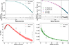 |
Fig. 5. Radial profiles of the model SZ (top left), X-ray SB (top right), X-ray temperature (bottom left), and tangential shear (bottom right) obtained from the accepted samples from the MCMC fit to Abell 1689. The dashed vertical black line on the X-ray SB profile indicates the radius at which the two-dimensional analysis (left) transitioned to a one-dimensional analysis (right). The radial profiles of the corresponding observational data are plotted alongside the models. The SZ and X-ray SB model profiles show close agreement to the observational data, so a ratio of the model to the observed data points is shown in the bottom portion of these plots. The profiles of the ICM observables are truncated at the value of R500c obtained by Planck Collaboration XXVII (2016), while the tangential shear extends past this. |
6.1. Geometry
We found axial ratios of  and qICM, 2 = 0.86 ± 0.03. The two axial ratios found in this work are higher than those found in K24. Our fit indicates that the major axis of Abell 1689 is almost perfectly aligned with the line of sight, with cos
 , in agreement with the K24 result. We found an elongation of ℛLP = 1.20 ± 0.04, which, when converted to the definition for elongation in K24, gives e∥ = 1.14 ± 0.04, which is ∼2σ lower than the value found in that work. We attribute these changes in geometry to the updates to the pipeline described in Appendix A.
6.2. Mass and concentration
For the total matter density profile, we recovered  [1014 M⊙] and
  . To gauge any potential bias introduced by projection effects, we also performed a spherical fit (qICM, 1 = qICM, 2 = 1) to the WL data within our pipeline to obtain
  [1014 M⊙] and
  . We show the posterior distributions of these triaxial and spherical values in Figure 6. Prior fits of spherical models have suggested a surprisingly high concentration for this system, consistent with our value of c200c, sph, and triaxiality and projection have been proposed as a possible explanation for such values (Broadhurst et al. 2008; Oguri et al. 2009; Sereno et al. 2010; Meneghetti et al. 2014). However, the high value of c200c is retained in our triaxial fit, suggesting that it may be intrinsic to the system rather than a result of projection. We also note that the informative log-normal prior influences the shape of our recovered posterior. In Figure 6, the right edge of the posterior distribution for c200c is set by the shape of the right edge of the prior. Performing the fit with flat prior (𝒰(0, 20)) on c200c returns a posterior distribution for this value that hits the upper end of the prior. Additionally, the exceptionally high concentration obtained in our fits aligns with known selection effects. That is, strong-lensing clusters tend to be biased toward compact, LOS-aligned configurations, such as Abell 1689. The much higher mass obtained in the spherical fit is in agreement with our expectations from the fitted geometry, given the recovered LOS elongation.
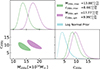 |
Fig. 6. Posterior distributions of the mass and concentration obtained for a fit to Abell 1689 using SZ, X-ray SB, and temperature, and WL data assuming a triaxial geometry (in green, labeled M200c, triax and c200c, triax) and using only WL data, assuming a spherical geometry (in purple, labeled M200c, sph and c200c, sph). The 68% credible regions for the two results are color-filled in the bottom left subplot. The log normal prior we applied to c200c, which depends on mass, is marginalized over the 68% credible bounds of M200c, triax and plotted in blue in the lower right subplot. Note that the prior is strongly informative and the upper edges of the posterior distributions for c200c are largely set by it. |
6.3. Nonthermal pressure
As discussed in Section 3, the calculation of the nonthermal pressure fraction was performed using the chains of accepted samples from the MCMC for the individual parameters. Figure 7 shows a radial plot of the recovered nonthermal pressure fraction Pnt/Ptot with the 68% credible region in purple. The radial range of this profile was set on the lower end by the WL data (∼180 kpc, see Section 5.2) and on the upper end by the maximum radius considered for the gas observables, (1.37 Mpc, see Section 5.1). We found that Pnt/Ptot has a value of ∼26% at the minimum considered radius, decreases to a minimum value of ∼18%t near 600 kpc, and then gradually increases to ∼30% at the maximal considered radius. Included in the plot is the nonthermal pressure fraction and 68% credible region obtained by Chappuis et al. (2025), found from their analysis of this same cluster. Additionally, we plot the nonthermal pressure fraction profiles from two independent analyses of an ensemble of simulated galaxy clusters in yellow (Sayers et al. 2021; Cui et al. 2018, The300) and green (Nelson et al. 2014, Omega500), along with their respective intrinsic cluster-to-cluster scatter.
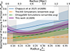 |
Fig. 7. Nonthermal pressure fraction (Pnt/Ptot) from our fit to Abell 1689, along with the corresponding 68% credible region (shaded purple), calculated from the accepted MCMC samples as outlined in Section 3. For comparison, the Pnt/Ptot result obtained for the same cluster by Chappuis et al. (2025) is shown in blue, also plotted with the corresponding 68% credible region. The results in yellow and green show the ensemble-average Pnt/Ptot result from independent analyses of simulated clusters from The300 (Sayers et al. 2021) and Omega500 (Nelson et al. 2014) simulations. The shaded hashed regions for these correspond to the 68% intrinsic cluster-to-cluster scatter within those simulations. Shaded gray denotes regions where the mass distribution may not be fully constrained from the observed WL shear signal (see Section 5.2). |
6.4. Gas-mass fraction
We show in Figure 8 the gas-mass fraction calculated from our fit to the electron density, converted into a gas density using Eq. (17), and the total density that we modeled as an NFW profile. From these, we obtained the three-dimensional integrated gas mass and total mass as functions of radius, and their ratio provides the gas-mass fraction. We compare our profile to that obtained from the ensemble average profile of simulated clusters from The300 (Cui et al. 2018) used in the analysis of Rasia et al. (2025) and we find good agreement at all radii. The shaded hashed region of the pink curve is the 68% intrinsic cluster-to-cluster scatter on the ensemble average. We also show the gas-mass fraction of five simulated clusters from the sample used in Rasia et al. (2025) that have similar mass-concentration relations (dashed purple lines) as what we find for Abell 1689. We note that our measured gas-mass fraction is also consistent with that found in a recent observational study from Eckert et al. (2019).
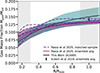 |
Fig. 8. Gas-mass fraction computed from our fits to the gas and total mass density (in blue) compared to the ensemble average profile obtained from simulated galaxy clusters from The300 (in pink) used in the analysis of Rasia et al. (2025). The 68% credible region and intrinsic scatter are shown in the shaded region of the respective profiles. We also show a matched sample of five simulated galaxy clusters used in the analysis of Rasia et al. (2025) that have a similar mass and concentration relation to Abell 1689 as dashed purple lines. Additionally, we compared to the result from Eckert et al. (2019), who provide the median value of the gas-mass fraction obtained from a sample of 12 observed galaxy clusters at R500c. Shaded gray denotes regions where the mass distribution may not be fully constrained from the observed WL shear signal (see Section 5.2). |
7. Discussion
K24 provides a detailed comparison of the axial ratios and inclination angle obtained from their triaxial fit to those found in other studies of Abell 1689 (Sereno et al. 2012; Umetsu et al. 2015). Because our results on the triaxial geometry are broadly in agreement with K24, we instead focus our discussion on comparing our total mass and nonthermal pressure results with those in the literature. In particular, we note that results from Chappuis et al. (2025) are especially relevant. They used identical one-dimensional observational datasets for the X-ray temperature and X-ray SB as used in this work, though their X-ray SB analysis employs this one-dimensional data at all radii. Additionally, we have confirmed that the azimuthally averaged SZ and X-ray SB data shown in Figure 5 are consistent with the corresponding one-dimensional projected profiles for those data used in Chappuis et al. (2025), which were derived using identical datasets from XMM-Newton and ACT DR6. We further note that the same underlying shape catalogs from Subaru were used in our WL analyses. Although, as noted above, Chappuis et al. (2025) considered the one-dimensional tangential shear profile while we fit the two-dimensional, two-component shear maps. With regard to overall three-dimensional geometry, Chappuis et al. (2025) find a LOS elongation of 1.30 ± 0.03, which is within ∼1.5σ of our value, ℛLP = 1.20 ± 0.04.
7.1. Mass and concentration
Similar analyses have been performed on Abell 1689 to obtain constraints on M200c and c200c on a spherical and triaxial basis. Our spherical mass and concentration results are consistent with the previous WL analysis of Abell 1689 by Umetsu & Broadhurst (2008), which found  and
and  , using WL shear and magnification data. Our results are also in agreement with the mass and concentration values found from a spherical WL-only analysis by Chappuis et al. (2025).
A summary of the results from previous analyses employing triaxial mass models are shown in Table 2 and described in detail below. In aggregate, we generally find excellent agreement with these prior studies.
-
Oguri et al. (2005) fit a triaxial NFW profile to a combined SL and WL dataset from HST and Subaru. They produced a model lensing convergence field for a triaxial halo that is specified by 7 parameters, which are the virial radius of the triaxial halo, the concentration, two axial ratios and three Euler angles. Flat priors are applied to all parameters. The virial mass is not a free parameter in the fit, but is derived from the model parameters. From their results, we calculated NFW-equivalent triaxial model parameters of M200c
 M⊙ and
  (Umetsu et al. 2015). Their M200c value is fully consistent with ours and our c200c values differ at a significance of 2σ.
 -
Sereno & Umetsu (2011) fit a triaxial NFW profile to a combined set of SL and WL data. The WL maps included shear plus magnification based on Subaru images and SL multiple image systems were derived from HST. Their model parameters and priors were identical to those fit by Oguri et al. (2005), and they found M200c =(13 ± 2)×1014 M⊙ and c200c = 7.3 ± 0.8. These values are fully consistent with our results. They also performed a WL-only triaxial fit that used priors on geometry from N-body simulations to find (13 ± 4)×1014 M⊙ and c200c = 10 ± 3, again, fully consistent with our results.
-
Morandi et al. (2011) performed a joint fit to X-ray (Chandra), WL (Subaru), and SL (HST) measurements. They assumed a gNFW triaxial model of the DM, with free parameters being the concentration, scale radius, the inner slope of the total matter profile, and two axial ratios. From their fit to this profile they found M200c =(25.9 ± 0.9)×1014 M⊙ and c200c = 5.71 ± 0.47. There is significant discrepancy between these values, our results, and other results found in the literature. However, we note that the deviation is closely aligned with the strong degeneracy direction between concentration and mass, suggesting that the true discrepancy is much lower than what is implied by the marginalized one-dimensional parameter values.
-
Sereno et al. (2013) used a multi-probe dataset comprised of a two-dimensional WL convergence map from Subaru, along with SL observations from HST, one-dimensional X-ray SB measured by Chandra, and one-dimensional X-ray temperature data obtained from spectroscopic fits to XMM-Newton data. Additionally, they considered the total integrated SZ signal obtained from combining data from 7 different facilities. They assumed an ellipsoidal NFW profile to describe the density distribution of total matter and fit for the mass, concentration, the two axial ratios of the matter distribution, the minor to major axial ratio of the ICM, and elongation and found M200c = (13.3 ± 1.7)×1014 M⊙ and c200c = 7.8 ± 0.7. These values are again consistent with our results.
-
Umetsu et al. (2015) combined WL data from Subaru with SL from HST, X-ray observations from Chandra and interferometric ground-based SZ data. Note that the WL data used in this work is deeper than that used in Sereno et al. (2013). They constructed the projected matter distribution from a joint WL analysis of two-dimensional shear and azimuthally integrated magnification constraints, assuming an elliptical NFW profile. Uniform priors were applied to the free parameters, which are the same as the above analysis. For their full multi-probe analysis, they found M200c =(17.8 ± 2.3)×1014 M⊙ and c200c = 8.36 ± 1.27, consistent with our findings.
While they did not perform a full three-dimensional triaxial analysis, we also compare with the findings of Chappuis et al. (2025), who, as noted earlier, used SZ, X-ray, and WL data products derived from the same pipeline as our work (CHEX-MATE Collaboration 2021). They found  M⊙ and
  , which are ∼1.5σ higher and within 1σ, respectively, relative to our results. Their model assumed a generalized HSE relation within the fit, allowing the ICM gas model to be connected to the total matter density model. This means that at small radii, the X-ray and SZ data provide a constraint on the total mass profile, and thus, on c200c. Compared to our results, along with those based on combining WL and SL, their result suggests that the gas probes favor a shallower inner mass profile than gravitational lensing. Prior results also imply that including SL data yields lower values of c200c. Furthermore, as with Morandi et al. (2011), our mass and concentration values differ along the primary degeneracy direction, suggesting that the true discrepancy in our results is smaller than what is implied by the one-dimensional marginalized parameter values. Finally, we note that their pipeline is able to obtain more precise constraints on the mass profile, primarily for c200c, as it was developed and optimized for such measurements with the inclusion of constraints from the gas data.
Published mass and concentration measurements of A1689.
7.2. Nonthermal pressure fraction
The level of nonthermal pressure support in Abell 1689 was addressed in two previous studies, both of which employed the same generalized HSE equation as we did to describe the thermal state of the cluster (i.e., Eq. (15)). These studies also assumed a triaxial basis. Specifically, Sereno et al. (2013) found the contribution of nonthermal pressure in Abell 1689 is ∼20–50% in the inner regions (≲300 kpc) and ∼25 ± 5% at ∼1.5 Mpc. Morandi et al. (2011) assumed a model of the nonthermal pressure of the gas that is a constant fraction of the total pressure and found a contribution on the order of ∼20%. Our derived nonthermal pressure support is consistent with these results, with a higher level of precision corresponding to a 68% credible region with a total spread of approximately 10% across the full radial range.
Chappuis et al. (2025) found a nonthermal pressure fraction equal to ∼20% at small radii and increasing steadily to ∼40% near the maximum radius considered in our analysis (see Figure 7). This result is consistent with ours at the 1σ level over the full radial range. The modest differences in radial shape between the profiles are a result of modeling differences. Chappuis et al. (2025) uses a parametric form of Pnt within their fit, constraining the overall shape of the profile (i.e., it must monotonically increase with radius). In our analysis the Pnt/Ptot profile was derived from a combination of the gas density, gas pressure, and total density profiles, and it can thus obtain a wide range of possible radial shapes. We obtained tighter constraints on our radial profile of the nonthermal pressure fraction than Chappuis et al. (2025), which we again attribute to modeling differences.
In Figure 7, we also display the nonthermal pressure fraction obtained from large samples of simulated clusters, in particular, The300 and the Omega500 simulations (Nelson et al. 2014). The analysis described in Sayers et al. (2021) was applied to 315 simulated clusters from The300 to obtain the ensemble average profile shown in yellow. The intrinsic cluster-to-cluster scatter for this sample is shown as the hashed yellow region. Over most of the radial range, the 68% credible region from our fit lies above the upper bound of the yellow hashed region, indicating that Abell 1689 has a somewhat higher than typical nonthermal pressure fraction relative to The300 clusters. The nonthermal pressure fraction plotted in green is from an analysis applied to 65 simulated clusters is presented in Nelson et al. (2014) from the Omega500 simulations. The intrinsic cluster-to-cluster scatter for this sample is shown as the hashed green region. For the full radial range considered, the value of Pnt/Ptot that we obtain for Abell 1689 is consistent with the ensemble average from the Omega500 clusters.
Additionally, we observe a minimum in the Pnt/Ptot profile at an intermediate radius near 600 kpc. This feature is not observed in the profile from Chappuis et al. (2025), but their parameterization does not allow for such a profile. In Section 4, we demonstrated that profiles of this shape can be recovered by our pipeline. To determine the statistical preference for such a minimum relative to a flat or monotonically increasing profile, we determined the fraction of Pnt/Ptot profiles calculated from the accepted samples of the MCMC chain that show a decrease between the minimum radius and 600 kpc. Approximately 77% of these profiles demonstrated this behavior, suggesting that the data have a mild preference for decreasing Pnt/Ptot between the central cluster region and intermediate radial values.
8. Conclusion
We presented an expansion of the triaxial modeling pipeline developed in K24, now including a WL analysis alongside the established SZ and X-ray analyses. The addition of WL enabled us to reconstruct the total matter density profile of a galaxy cluster and to measure its nonthermal pressure profile, all within a triaxial framework. The pipeline was validated on a range of mock observations generated from smooth models to verify our ability to constrain mass, concentration, elongation, and the underlying Pnt/Ptot profile. We plan to apply this pipeline to a large sample of mock observations taken from The300 simulations (Cui et al. 2018) to further assess any bias in the modeling assumptions and fitting mechanism when applied to more realistic data.
We demonstrated this multi-probe analysis on the CHEX-MATE galaxy cluster Abell 1689 and obtained measurements of its intrinsic three-dimensional shape, mass, and nonthermal pressure fraction. This cluster is elongated along the LOS, with an elongation of ℛLP = 1.20 ± 0.04, in agreement with K24 and Chappuis et al. (2025). We measured a mass in our triaxial framework of  [1014 M⊙] and a corresponding concentration of
  . The value obtained for c200c is unusually high for a cluster of this mass, but we found that this high value was retained when a fit assuming a spherical model using WL data alone was performed. We therefore conclude that this high concentration is not due to projection effects and is intrinsic to the cluster. On the other hand, the spherical model returned a higher mass value, higher by ∼2σ, demonstrating the bias introduced by the spherical model due to the strong degeneracy between total mass and elongation along the LOS (e.g., Meneghetti et al. 2010b; Euclid Collaboration: Giocoli et al. 2024). This is a strong motivation for the future application of our method to the full CHEX-MATE sample because to date, the WL mass bias due to the assumption of spherical symmetry has yet to be quantified from an observational analysis of a large sample of clusters. For the profile of Pnt/Ptot, we obtained results that agree with Chappuis et al. (2025) at all radii, with an uncertainty level of 10%. We also found agreement with the ensemble average profile from the Omega500 simulations Nelson et al. (2014), but an analysis of the full CHEX-MATE sample is necessary for a true comparison.
Acknowledgments
This research was supported by the International Space Science Institute (ISSI) in Bern, through ISSI International Team project #565 (Multi-Wavelength Studies of the Culmination of Structure Formation in the Universe). AG, JS, HS and JK were supported by NASA Astrophysics Data Analysis Program (ADAP) Grant 80NSSC21K1571. S.E., M.S., M.R., HB, FDL, PM, ... acknowledge the financial contribution from the contracts Prin-MUR 2022 supported by Next Generation EU (M4.C2.1.1, n.20227RNLY3 The concordance cosmological model: stress-tests with galaxy clusters), and from the European Union’s Horizon 2020 Programme under the AHEAD2020 project (grant agreement n. 871158). LL acknowledges the financial contribution from the INAF grant 1.05.12.04.01. M.G. acknowledges support from the ERC Consolidator Grant BlackHoleWeather (101086804). MS acknowledges the financial contributions from contract INAF mainstream project 1.05.01.86.10 and INAF Theory Grant 2023: Gravitational lensing detection of matter distribution at galaxy cluster boundaries and beyond (1.05.23.06.17). HB, FDL, and PM acknowledge support by the Fondazione ICSC, Spoke 3 Astrophysics and Cosmos Observations. National Recovery and Resilience Plan (Piano Nazionale di Ripresa e Resilienza, PNRR) Project ID CN_00000013 “Italian Research Center on High-Performance Computing, Big Data and Quantum Computing” funded by MUR Missione 4 Componente 2 Investimento 1.4: Potenziamento strutture di ricerca e creazione di “campioni nazionali di R&S (M4C2-19 )” – Next Generation EU (NGEU), by INFN through the InDark initiative. DE acknowledges support from the Swiss National Science Foundation (SNSF) under grant agreement 200021_212576. K.U. acknowledges support from the National Science and Technology Council of Taiwan (grant NSTC 112-2112-M-001-027-MY3) and the Academia Sinica Investigator Award (grant AS-IA-112-M04). This research was supported by Basic Science Research Program through the National Research Foundation of Korea (NRF) funded by the Ministry of Education (2019R1A6A1A10073887). This research was funded by the 2025 KAIST-U.S. Joint Research Collaboration Open Track Project for Early-Career Researchers, supported by the International Office at the Korea Advanced Institute of Science and Technology (KAIST).
References
- Aguena, M., Aiola, S., Allam, S., et al. 2026, Open J. Astrophys., 9, 55863 [Google Scholar]
- Allgood, B., Flores, R. A., Primack, J. R., et al. 2006, MNRAS, 367, 1781 [NASA ADS] [CrossRef] [Google Scholar]
- Angelinelli, M., Vazza, F., Giocoli, C., et al. 2020, MNRAS, 495, 864 [NASA ADS] [CrossRef] [Google Scholar]
- Applegate, D. E., von der Linden, A., Kelly, P. L., et al. 2014, MNRAS, 439, 48 [Google Scholar]
- Arnaud, K. A. 1996, ASP Conf. Ser., 101, 17 [Google Scholar]
- Arnaud, M., Pratt, G. W., Piffaretti, R., et al. 2010, A&A, 517, A92 [CrossRef] [EDP Sciences] [Google Scholar]
- Bailin, J., & Steinmetz, M. 2005, ApJ, 627, 647 [Google Scholar]
- Bartalucci, I., Molendi, S., Rasia, E., et al. 2023, A&A, 674, A179 [NASA ADS] [CrossRef] [EDP Sciences] [Google Scholar]
- Bertin, E. 2006, ASP Conf. Ser., 351, 112 [NASA ADS] [Google Scholar]
- Bertin, E. 2010, Astrophysics Source Code Library [record ascl:1010.063] [Google Scholar]
- Bertin, E. 2011, ASP Conf. Ser., 442, 435 [Google Scholar]
- Bertin, E., Mellier, Y., Radovich, M., et al. 2002, ASP Conf. Ser., 281, 228 [Google Scholar]
- Bett, P., Eke, V., Frenk, C. S., et al. 2007, MNRAS, 376, 215 [NASA ADS] [CrossRef] [Google Scholar]
- Bleem, L. E., Klein, M., Abbot, T. M. C., et al. 2024, Open J. Astrophys., 7, 13 [CrossRef] [Google Scholar]
- Bonamigo, M., Despali, G., Limousin, M., et al. 2015, MNRAS, 449, 3171 [NASA ADS] [CrossRef] [Google Scholar]
- Bond, J. R., Kofman, L., & Pogosyan, D. 1996, Nature, 380, 603 [NASA ADS] [CrossRef] [Google Scholar]
- Broadhurst, T., Umetsu, K., Medezinski, E., Oguri, M., & Rephaeli, Y. 2008, ApJ, 685, L9 [Google Scholar]
- Cappellari, M., & Copin, Y. 2003, MNRAS, 342, 345 [Google Scholar]
- Chappuis, L., Eckert, D., Sereno, M., et al. 2025, A&A, 699, A141 [NASA ADS] [CrossRef] [EDP Sciences] [Google Scholar]
- CHEX-MATE Collaboration (Arnaud, M., et al.) 2021, A&A, 650, A104 [NASA ADS] [CrossRef] [EDP Sciences] [Google Scholar]
- Chiu, I. N., Umetsu, K., Sereno, M., et al. 2018, ApJ, 860, 126 [NASA ADS] [CrossRef] [Google Scholar]
- Chiu, I.-N., Ghirardini, V., Grandis, S., et al. 2025, A&A, 704, A110 [NASA ADS] [CrossRef] [EDP Sciences] [Google Scholar]
- Cole, S., & Lacey, C. 1996, MNRAS, 281, 716 [NASA ADS] [CrossRef] [Google Scholar]
- Coulton, W., Madhavacheril, M. S., Duivenvoorden, A. J., et al. 2024, Phys. Rev. D, 109, 063530 [NASA ADS] [CrossRef] [Google Scholar]
- Cui, W., Knebe, A., Yepes, G., et al. 2018, MNRAS, 480, 2898 [Google Scholar]
- Davis, M., Efstathiou, G., Frenk, C. S., & White, S. D. M. 1985, ApJ, 292, 371 [Google Scholar]
- De Filippis, E., Sereno, M., Bautz, M. W., & Longo, G. 2005, ApJ, 625, 108 [NASA ADS] [CrossRef] [Google Scholar]
- Despali, G., Giocoli, C., & Tormen, G. 2014, MNRAS, 443, 3208 [Google Scholar]
- Diehl, S., & Statler, T. S. 2006, MNRAS, 368, 497 [NASA ADS] [CrossRef] [Google Scholar]
- Diemer, B. 2018, ApJS, 239, 35 [NASA ADS] [CrossRef] [Google Scholar]
- Diemer, B., & Joyce, M. 2019, ApJ, 871, 168 [NASA ADS] [CrossRef] [Google Scholar]
- Dubinski, J., & Carlberg, R. G. 1991, ApJ, 378, 496 [Google Scholar]
- Eckert, D., Roncarelli, M., Ettori, S., et al. 2015, MNRAS, 447, 2198 [Google Scholar]
- Eckert, D., Ghirardini, V., Ettori, S., et al. 2019, A&A, 621, A40 [NASA ADS] [CrossRef] [EDP Sciences] [Google Scholar]
- Eckert, D., Finoguenov, A., Ghirardini, V., et al. 2020, Open J. Astrophys., 3, 12 [NASA ADS] [CrossRef] [Google Scholar]
- Ettori, S. 2000, MNRAS, 311, 313 [NASA ADS] [CrossRef] [Google Scholar]
- Ettori, S., Morandi, A., Tozzi, P., et al. 2009, A&A, 501, 61 [NASA ADS] [CrossRef] [EDP Sciences] [Google Scholar]
- Euclid Collaboration (Giocoli, C., et al.) 2024, A&A, 681, A67 [NASA ADS] [CrossRef] [EDP Sciences] [Google Scholar]
- Euclid Collaboration (Martinet, N., et al.) 2019, A&A, 627, A59 [NASA ADS] [CrossRef] [EDP Sciences] [Google Scholar]
- Foreman-Mackey, D., Hogg, D. W., Lang, D., & Goodman, J. 2013, PASP, 125, 306 [Google Scholar]
- Fox, D. C., & Pen, U.-L. 2002, ApJ, 574, 38 [NASA ADS] [CrossRef] [Google Scholar]
- Frenk, C. S., White, S. D. M., Davis, M., & Efstathiou, G. 1988, ApJ, 327, 507 [NASA ADS] [CrossRef] [Google Scholar]
- Gao, L., Navarro, J. F., Frenk, C. S., et al. 2012, MNRAS, 425, 2169 [NASA ADS] [CrossRef] [Google Scholar]
- Gaspari, M., Tombesi, F., & Cappi, M. 2020, Nat. Astron., 4, 10 [Google Scholar]
- Ghirardini, V., Eckert, D., Ettori, S., et al. 2019, A&A, 621, A41 [NASA ADS] [CrossRef] [EDP Sciences] [Google Scholar]
- Goodman, J., & Weare, J. 2010, Commun. Appl. Math. Comput. Sci., 5, 65 [Google Scholar]
- Hilton, M., Sifón, C., Naess, S., et al. 2021, ApJS, 253, 3 [Google Scholar]
- Hinshaw, G., Larson, D., Komatsu, E., et al. 2013, ApJS, 208, 19 [Google Scholar]
- Hoekstra, H. 2003, MNRAS, 339, 1155 [NASA ADS] [CrossRef] [Google Scholar]
- Hoekstra, H., Herbonnet, R., Muzzin, A., et al. 2015, MNRAS, 449, 685 [NASA ADS] [CrossRef] [Google Scholar]
- Hogg, D. W., & Foreman-Mackey, D. 2018, ApJS, 236, 11 [NASA ADS] [CrossRef] [Google Scholar]
- Hopkins, P. F., Bahcall, N. A., & Bode, P. 2005, ApJ, 618, 1 [NASA ADS] [CrossRef] [Google Scholar]
- Hu, W., & White, M. 2001, ApJ, 554, 67 [Google Scholar]
- Jing, Y. P., & Suto, Y. 2002, ApJ, 574, 538 [Google Scholar]
- Kaiser, N. 1986, MNRAS, 222, 323 [Google Scholar]
- Kaiser, N. 1991, ApJ, 383, 104 [NASA ADS] [CrossRef] [Google Scholar]
- Kaiser, N. 1992, ApJ, 388, 272 [Google Scholar]
- Kasun, S. F., & Evrard, A. E. 2005, ApJ, 629, 781 [NASA ADS] [CrossRef] [Google Scholar]
- Kennel, M. B. 2004, arXiv e-prints [arXiv:physics/0408067] [Google Scholar]
- Khatri, R., & Gaspari, M. 2016, MNRAS, 463, 655 [Google Scholar]
- Kim, J., Sayers, J., Sereno, M., et al. 2024, A&A, 686, A97 [NASA ADS] [CrossRef] [EDP Sciences] [Google Scholar]
- Kravtsov, A. V., & Borgani, S. 2012, ARA&A, 50, 353 [Google Scholar]
- Kuntz, K. D., & Snowden, S. L. 2008, A&A, 478, 575 [NASA ADS] [CrossRef] [EDP Sciences] [Google Scholar]
- Laigle, C., McCracken, H. J., Ilbert, O., et al. 2016, ApJS, 224, 24 [Google Scholar]
- Lau, E. T., Kravtsov, A. V., & Nagai, D. 2009, ApJ, 705, 1129 [NASA ADS] [CrossRef] [Google Scholar]
- Lau, E. T., Nagai, D., Kravtsov, A. V., & Zentner, A. R. 2011, ApJ, 734, 93 [CrossRef] [Google Scholar]
- Lau, E. T., Nagai, D., Kravtsov, A. V., Vikhlinin, A., & Zentner, A. R. 2012, ApJ, 755, 116 [NASA ADS] [CrossRef] [Google Scholar]
- Limousin, M., Morandi, A., Sereno, M., et al. 2013, Space Sci. Rev., 177, 155 [Google Scholar]
- Lovisari, L., Ettori, S., Rasia, E., et al. 2024, A&A, 682, A45 [NASA ADS] [CrossRef] [EDP Sciences] [Google Scholar]
- Mandelbaum, R., Rowe, B., Armstrong, R., et al. 2015, MNRAS, 450, 2963 [Google Scholar]
- Mazzotta, P., Rasia, E., Moscardini, L., & Tormen, G. 2004, MNRAS, 354, 10 [NASA ADS] [CrossRef] [Google Scholar]
- McNamara, B. R., Nulsen, P. E. J., Wise, M. W., et al. 2005, Nature, 433, 45 [NASA ADS] [CrossRef] [PubMed] [Google Scholar]
- Medezinski, E., Broadhurst, T., Umetsu, K., et al. 2010, MNRAS, 405, 257 [NASA ADS] [Google Scholar]
- Medezinski, E., Oguri, M., Nishizawa, A. J., et al. 2018, PASJ, 70, 30 [NASA ADS] [Google Scholar]
- Meneghetti, M., Fedeli, C., Pace, F., Gottlöber, S., & Yepes, G. 2010a, A&A, 519, A90 [NASA ADS] [CrossRef] [EDP Sciences] [Google Scholar]
- Meneghetti, M., Rasia, E., Merten, J., et al. 2010b, A&A, 514, A93 [NASA ADS] [CrossRef] [EDP Sciences] [Google Scholar]
- Meneghetti, M., Rasia, E., Vega, J., et al. 2014, ApJ, 797, 34 [Google Scholar]
- Miniati, F., Ryu, D., Kang, H., et al. 2000, ApJ, 542, 608 [NASA ADS] [CrossRef] [Google Scholar]
- Morandi, A., & Limousin, M. 2012, MNRAS, 421, 3147 [Google Scholar]
- Morandi, A., Limousin, M., Rephaeli, Y., et al. 2011, MNRAS, 416, 2567 [NASA ADS] [CrossRef] [Google Scholar]
- Morandi, A., Limousin, M., Sayers, J., et al. 2012, MNRAS, 425, 2069 [NASA ADS] [CrossRef] [Google Scholar]
- Muñoz-Cuartas, J. C., Macciò, A. V., Gottlöber, S., & Dutton, A. A. 2011, MNRAS, 411, 584 [Google Scholar]
- Naess, S., Guan, Y., Duivenvoorden, A. J., et al. 2025, JCAP, 2025, 061 [Google Scholar]
- Nagai, D., Kravtsov, A. V., & Vikhlinin, A. 2007, ApJ, 668, 1 [Google Scholar]
- Navarro, J. F., Frenk, C. S., & White, S. D. M. 1997, ApJ, 490, 493 [Google Scholar]
- Nelson, K., Lau, E. T., & Nagai, D. 2014, ApJ, 792, 25 [NASA ADS] [CrossRef] [Google Scholar]
- Oguri, M., Takada, M., Umetsu, K., & Broadhurst, T. 2005, ApJ, 632, 841 [Google Scholar]
- Oguri, M., Hennawi, J. F., Gladders, M. D., et al. 2009, ApJ, 699, 1038 [NASA ADS] [CrossRef] [Google Scholar]
- Oguri, M., Takada, M., Okabe, N., & Smith, G. P. 2010, MNRAS, 405, 2215 [NASA ADS] [Google Scholar]
- Paz, D. J., Lambas, D. G., Padilla, N., & Merchán, M. 2006, MNRAS, 366, 1503 [Google Scholar]
- Pearce, F. A., Kay, S. T., Barnes, D. J., Bower, R. G., & Schaller, M. 2020, MNRAS, 491, 1622 [NASA ADS] [CrossRef] [Google Scholar]
- Piffaretti, R., & Valdarnini, R. 2008, A&A, 491, 71 [NASA ADS] [CrossRef] [EDP Sciences] [Google Scholar]
- Planck Collaboration XXVII. 2016, A&A, 594, A27 [NASA ADS] [CrossRef] [EDP Sciences] [Google Scholar]
- Pointecouteau, E., Santiago-Bautista, I., Douspis, M., et al. 2021, A&A, 651, A73 [NASA ADS] [CrossRef] [EDP Sciences] [Google Scholar]
- Postman, M., Coe, D., Benítez, N., et al. 2012, ApJS, 199, 25 [Google Scholar]
- Rasia, E., Tripodi, R., Borgani, S., et al. 2025, A&A, 702, A182 [NASA ADS] [CrossRef] [EDP Sciences] [Google Scholar]
- Romero, C. E., Gaspari, M., Schellenberger, G., et al. 2025, ApJ, 985, 248 [Google Scholar]
- Roncarelli, M., Ettori, S., Borgani, S., et al. 2013, MNRAS, 432, 3030 [NASA ADS] [CrossRef] [Google Scholar]
- Rossetti, M., Eckert, D., Gastaldello, F., et al. 2024, A&A, 686, A68 [NASA ADS] [CrossRef] [EDP Sciences] [Google Scholar]
- Sarazin, C. L. 1986, Rev. Mod. Phys., 58, 1 [Google Scholar]
- Sarkar, A., McDonald, M., Bleem, L., et al. 2025, ApJ, 984, L63 [Google Scholar]
- Sayers, J., Golwala, S. R., Ameglio, S., & Pierpaoli, E. 2011, ApJ, 728, 39 [NASA ADS] [CrossRef] [Google Scholar]
- Sayers, J., Sereno, M., Ettori, S., et al. 2021, MNRAS, 505, 4338 [NASA ADS] [CrossRef] [Google Scholar]
- Sayers, J., Mantz, A. B., Rasia, E., et al. 2023, ApJ, 944, 221 [NASA ADS] [CrossRef] [Google Scholar]
- Schneider, P., van Waerbeke, L., Kilbinger, M., & Mellier, Y. 2002, A&A, 396, 1 [NASA ADS] [CrossRef] [EDP Sciences] [Google Scholar]
- Seitz, C., & Schneider, P. 1997, A&A, 318, 687 [NASA ADS] [Google Scholar]
- Sereno, M., & Umetsu, K. 2011, MNRAS, 416, 3187 [NASA ADS] [CrossRef] [Google Scholar]
- Sereno, M., De Filippis, E., Longo, G., & Bautz, M. W. 2006, ApJ, 645, 170 [NASA ADS] [CrossRef] [Google Scholar]
- Sereno, M., Jetzer, P., & Lubini, M. 2010, MNRAS, 403, 2077 [Google Scholar]
- Sereno, M., Ettori, S., & Baldi, A. 2012, MNRAS, 419, 2646 [NASA ADS] [CrossRef] [Google Scholar]
- Sereno, M., Ettori, S., Umetsu, K., & Baldi, A. 2013, MNRAS, 428, 2241 [NASA ADS] [CrossRef] [Google Scholar]
- Sereno, M., Ettori, S., Meneghetti, M., et al. 2017, MNRAS, 467, 3801 [NASA ADS] [CrossRef] [Google Scholar]
- Sereno, M., Umetsu, K., Ettori, S., et al. 2018, ApJ, 860, L4 [NASA ADS] [CrossRef] [Google Scholar]
- Shi, X., & Komatsu, E. 2014, MNRAS, 442, 521 [NASA ADS] [CrossRef] [Google Scholar]
- Shi, X., Komatsu, E., Nelson, K., & Nagai, D. 2015, MNRAS, 448, 1020 [NASA ADS] [CrossRef] [Google Scholar]
- Siegel, S. R., Sayers, J., Mahdavi, A., et al. 2018, ApJ, 861, 71 [Google Scholar]
- Skrutskie, M. F., Cutri, R. M., Stiening, R., et al. 2006, AJ, 131, 1163 [NASA ADS] [CrossRef] [Google Scholar]
- Snowden, S. L., Mushotzky, R. F., Kuntz, K. D., & Davis, D. S. 2008, A&A, 478, 615 [NASA ADS] [CrossRef] [EDP Sciences] [Google Scholar]
- Stapelberg, S., Tchernin, C., Hug, D., Lau, E. T., & Bartelmann, M. 2022, A&A, 663, A17 [NASA ADS] [CrossRef] [EDP Sciences] [Google Scholar]
- Sunyaev, R. A., & Zeldovich, Y. B. 1972, Comm. Astrophys. Space Phys., 4, 173 [Google Scholar]
- Tashiro, M., Kelley, R., Watanabe, S., et al. 2025, PASJ, 77, S1 [Google Scholar]
- Umetsu, K. 2020, A&ARv, 28, 7 [Google Scholar]
- Umetsu, K., & Broadhurst, T. 2008, ApJ, 684, 177 [Google Scholar]
- Umetsu, K., Medezinski, E., Nonino, M., et al. 2012, ApJ, 755, 56 [NASA ADS] [CrossRef] [Google Scholar]
- Umetsu, K., Medezinski, E., Nonino, M., et al. 2014, ApJ, 795, 163 [NASA ADS] [CrossRef] [Google Scholar]
- Umetsu, K., Sereno, M., Medezinski, E., et al. 2015, ApJ, 806, 207 [NASA ADS] [CrossRef] [Google Scholar]
- Umetsu, K., Ueda, S., Hsieh, B.-C., et al. 2022, ApJ, 934, 169 [NASA ADS] [CrossRef] [Google Scholar]
- Vazza, F., Angelinelli, M., Jones, T. W., et al. 2018, MNRAS, 481, L120 [NASA ADS] [CrossRef] [Google Scholar]
- Vikhlinin, A., Kravtsov, A., Forman, W., et al. 2006, ApJ, 640, 691 [Google Scholar]
- Warren, M. S., Quinn, P. J., Salmon, J. K., & Zurek, W. H. 1992, ApJ, 399, 405 [NASA ADS] [CrossRef] [Google Scholar]
- XRISM Collaboration (Audard, M., et al.) 2025a, PASJ, 77, S242 [Google Scholar]
- XRISM Collaboration (Audard, M., et al.) 2025b, ApJ, 982, L5 [Google Scholar]
- XRISM Collaboration (Audard, M., et al.) 2025c, ApJ, 985, L20 [Google Scholar]
- XRISM Collaboration(Audard, M., et al.) 2025d, Nature, 638, 365 [Google Scholar]
- Zhuravleva, I., Churazov, E., Kravtsov, A., et al. 2013, MNRAS, 428, 3274 [NASA ADS] [CrossRef] [Google Scholar]
Appendix A: Updates relative to K24
The fitting pipeline used in this analysis expands upon the one initially created by K24. During the process of integrating the WL analysis into the established pipeline and performing cross checks of our results with similar analyses, namely the one by Chappuis et al. (2025), several updates were made to the algorithms described in K24. In addition, we have also used different observational data for some of the probes. Here we address each of the changes and discuss how they impact the fit. In several cases, we use the value of ℛLP to quantify the overall impact of the update on our analysis relative to that of K24. When considering all of the updates, the result is that ℛLP is approximately unchanged, and so we obtain overall consistent results with K24 as detailed in Section 6.
ACT DR6 data release Subsequent to the analysis of K24, the ACT DR6 maps were made publicly available (Coulton et al. 2024; Naess et al. 2025). The ACT DR6 maps are deeper than the DR4 maps used by K24, which results in more precise constraints on the electron pressure profile in our analysis. Consequently, as noted in Section 6, the SZ data dominate over the X-ray temperature data in constraining the shape of the pressure profile. With this new data release, we also updated the method used to calculate the covariance matrix, with the primary change being a masking of map regions that contain ACT cluster detections from Hilton et al. (2021). This results in a more accurate estimate of the (now lower) noise in the SZ Compton-y map.
Projected one-dimensional X-ray SB While we adopted an identical approach to K24 in using a projected one-dimensional X-ray SB profile at large radii, we obtained this profile in a different manner. Specifically, we used the azimuthal-median profiles calculated by Bartalucci et al. (2023). In contrast, K24 computed the projected profile from the azimuthal mean of the two-dimensional SB map. In addition, we discovered that the calculation of the associated uncertainties on this profile in K24 was incorrect, and had been inflated by an amount that approximately corresponds to the square root of the number of map pixels within each radial bin. As a result, the large-radius X-ray SB data were effectively down-weighted in the fit of K24, due to error estimates that were inflated by 1–2 orders of magnitude, and this resulted in a fit that was systematically lower than the observed data at those radii. The difference occurs at radii ≳3.5′, increasing to a factor of 2 at 5′and a factor of 10 at the maximum radius 7.4′. In aggregate, we found that the higher electron density recovered in our fit compared to that of K24 results in the value of ℛLP decreasing by approximately 0.05.
Projected one-dimensional X-ray temperature In their fit, K24 used the two-dimensional X-ray temperature map produced by Lovisari et al. (2024). As part of our testing, we compared the results obtained from this approach to those obtained from the projected one-dimensional temperature profiles from Rossetti et al. (2024), finding fitted temperature values approximately 10% higher from the one-dimensional profiles. As a result, this change reduced the value of ℛLP found in our analysis relative to that of K24 by approximately 0.20. We attribute this to the different weighting employed in the POS. In the case of the two-dimensional maps, the POS weighting is performed by the χ2 statistic used in the fit, and so it is an inverse-variance weighting. In contrast, the one-dimensional projected profiles are obtained from X-ray spectral fits to all the photons within a given annulus, which implies a weighting more similar to that suggested by Mazzotta et al. (2004). As shown by the comparisons in Lovisari et al. (2024), per-cluster differences comparable to the 10% value we obtained for Abell 1689 are expected for these different weighting choices. Lacking a definitive test to establish which approach is least biased, we chose to use the projected one-dimensional profiles for this analysis, since those are the default temperature products produced within the CHEX-MATE collaboration. This multiplicative difference in temperature primarily impacted the fitted LOS elongation, as quantified below when describing the change in APEC normalization.
Logarithmically spaced LOS projection integral In the development of the WL analysis, we found that the central values of the shear maps were unphysical when using a linear spacing for the numerical LOS integration of the three-dimensional elliptical coordinate. This was a result of the projection integration in Eq. (2), which was not sufficiently sampled at small radii. To remedy this, we updated the numerical integration to use log-spaced steps, with Eq. (2) becoming
 (A.1)
(A.1)
This change was also propagated to the SZ and X-ray SB projection integrals. The X-ray temperature calculation does not employ the log-spaced integral, since its value is far more uniform as a function of radius. Cross-checks were performed to ensure the log-spaced numerical integrals produce results consistent with the original linear-spaced numerical integrals for the gas quantities. Using a logarithmic basis decreased the integration time by three orders of magnitude for the SZ projection and by an order of magnitude for the X-ray SB projection relative to the linear basis. The fitted parameter values are not noticeably impacted by this update.
Tolerance of the numerical LOS projection integral To perform the numerical integration in Eq. 2, we use scipy.integrate.quad. This function allows for adjustment of the absolute and relative error tolerances. We found that when using the DR6 SZ map, to produce stable model maps the absolute and relative error tolerances needed to be adjusted from their default values of 1.49 × 10⁻⁸ to 10−12. Stability was defined as model maps that vary by less than 0.01% when the tolerances were lowered by an order of magnitude. We tested the model maps corresponding to the other observables and found the default tolerances were sufficient for them, so, to conserve computation time, the tolerance adjustment was only applied to the numerical projection integral corresponding to the SZ signal. This adjustment resulted in an overall decrease in the value of ℛLP by 0.03.
XMM-Newton vignetting correction When constructing the projected X-ray SB maps and profiles from the triaxial model, K24 inadvertently applied a vignetting to mimic the XMM-Newton response prior to comparing with the observed data. However, since the observed X-ray SB data have already been corrected for vignetting, this should not have been done, and it has now been removed from the analysis. In addition, the radial scaling of the vignetting correction was not correctly applied in K24. In aggregate, our updates to the vignetting correction resulted in the value of ℛLP increasing by 0.02.
APEC normalization In K24, an additional factor of (1 + z)−1 was mistakenly included when using the Python package pyproffit to calculate the emissivity. This error occurred because the package expects an input X-ray SB in units of the APEC normalization, which scales as (1 + z)−2, rather than the scaling of (1 + z)−3 from Eq. 4. Thus, the normalization in K24 was mis-estimated by a factor of 1.18. Correcting for this resulted in the value of ℛLP increasing by 0.18 in our analysis relative to K24.
XMM response file As described in Section 2.1, to calculate the emissivity, the XMM-Newton instrument response within the chosen energy band must be accounted for. K24 inadvertently used the incorrect ARF for these data. For the analysis in this paper, we instead used an approximately universal XMM-Newton ARF that is expected to be accurate for the observations of the CHEX-MATE clusters at the percent level. These two ARFs differ by approximately 7%, which resulted in our fitted value of ℛLP being larger by 0.07 relative to K24.
Beam convolution In order to convolve the two-dimensional model SZ and X-ray maps with their respective instrument beam PSFs, padding must be added to the maps so that they extend beyond R500c. K24 implemented zero-value padding, which we found introduced edge effects when the convolution was performed. To remedy this, we extended the overall size of the model maps prior to the convolution, so the padding was instead dictated by the ICM profiles. This change has increased the elongation by 0.08 relative to K24.
ACT covariance In K24 a fully diagonal ACT covariance matrix was unintentionally used for the χ2 calculation for the SZ portion of the analysis. In general, we calculated the ACT pixel covariance matrix from 10,000 randomly selected, independent patches in the ACT observing field the cluster is located in Pointecouteau et al. (2021), while avoiding areas that contain signal from clusters and point sources using the masks provided by Aguena et al. (2026). The patches used in this calculation match the size of the cluster’s SZ map. K24 inadvertently populated the patches with randomly selected ACT map pixels, rather than (N × N) ACT map cut-outs, thus losing off diagonal covariance terms. We found, through testing on fits to mock observations, that the diagonal covariance matrix does not adequately cover the expected fluctuations in recovered parameter values. So, we updated our analysis to use the full ACT covariance matrix in our model. However, we found when using the method described above to compute this, the inversion of the covariance matrix was numerically unstable and caused the fit to fail. To obtain a numerically stable version, we conditioned the covariance matrix by fitting a smooth model to the average covariance calculated from the 10,000 patches as a function of pixel separation. This is shown in Figure A.1. The inner points were fit by a decaying exponential and the outer points by a Gaussian. We used the sum of the two fit functions to reconstruct the covariance matrix. The inverse of this conditioned covariance matrix is numerically stable and was tested to ensure it captures the expected fluctuations in recovered parameter values. The results presented in this analysis employ this conditioned covariance matrix and this change resulted in the elongation decreasing by 0.04 relative to K24.
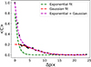 |
Fig. A.1. The function used to reconstruct a smooth, conditioned SZ ACT DR6 covariance matrix is shown in purple. It is constructed from an exponential fit (green dashed line) to the inner most black data points and a gaussian fit (red dashed line) to the outer black data points. The black data points were obtained by taking the average of the two-dimensional (unconditioned) covariance matrix in annular bins. |
Appendix B: Parameter degeneracies in the ICM model
Nagai et al. (2007) note that there are strong degeneracies between the pressure profile parameters, which generally prevent meaningful constraints when all are varied, so we fixed the value c500 to 1.4 and γp to 0.3, following Sayers et al. (2023). Additionally, for the demonstration in this paper, described in Section 5, the X-ray and SZ data are only fitted within the value of R500c derived by Planck, equal to 7.4′ (1.37 Mpc, Planck Collaboration XXVII 2016). The parameter βp primarily influences the shape of the pressure profile beyond this radius, and it is thus not well constrained by this analysis. We therefore used the parameterization for βp from Sayers et al. (2023), and so consequently our model has only two free parameters, P0 and αp. To better assess if the resulting parametrization of the pressure profile adequately describes the observed data, we performed a series of tests to determine if an additional third free parameter is justified based on the F-statistic. In brief, we found that none of the considered permutations of three free parameters in Pe(ζ) resulted in a statistically significant improvement in fit quality compared to the baseline fit with two free parameters, quantified by p-values ≥0.2 in all cases.
Appendix C: Recovered parameters to mock datasets
Here we summarize the results from all the fits to the mock datasets in Tables C.1, C.2 and C.3. The relevant best fit parameters from each fit are listed in the tables below. We also show the corner plot for the fit to the mock data shown in Figure C.1.
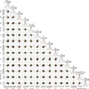 |
Fig. C.1. Posterior distributions estimated from our MCMC for a mock observation generated from a smooth model. The green vertical lines in each plot indicate the input parameters used to generate the mock observation maps and the red vertical lines represent the median value from the accepted MCMC samples. The value displayed above each histogram shows the median of the distribution, along with the 1σ (68%) credible region, which is indicated by the dashed vertical lines in every plot. The black line in the two-dimensional distributions encloses the 68% credible region. |
Recovered parameters from fits to mock dataset A
Recovered parameters from fits to mock dataset B
Recovered parameters from fits to mock dataset C
Appendix D: Tangential shear calculation
While our fit is based on the two-dimensional projected two-component shear (γ1 and γ2), we also constructed one-dimensional radial profiles of the tangential shear to better enable visual comparisons between the observed data and model (see Section 6). We briefly summarize here our calculation of the tangential shear. For more details, see Umetsu (2020). In a polar coordinate basis (θ, ϕ) centered on the lens, the shear signal can be deconstructed into two components, the tangential shear γ+, and the 45° rotated cross shear γ×:
 (D.1)
(D.1)
For an arbritary choice of the coordinate center, the azimuthally averaged components of the tangential and cross shear are expressed as (e.g., Umetsu 2020)
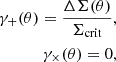 (D.2)
(D.2)
where 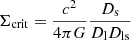 , and we have introduced the excess surface mass density ΔΣ(θ), defined as the difference between the average surface mass density
  within a circle of radius θ and the local surface mass density:
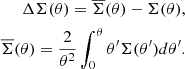 (D.3)
(D.3)
The tangential reduced shear is then defined as
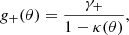 (D.4)
(D.4)
where we calculate the convergence as κ = Σ/Σcrit. Because triaxial halos have elliptical isodensity contours in projection on the sky, Eq. D.4 gives a good approximation to the WL signal for regular clusters (Umetsu 2020). To compare our model to the observed tangential shear data, we calculated the mean tangential shear in the nonlinear regime using the formulation of Seitz & Schneider (1997):
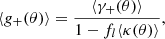 (D.5)
(D.5)
with
 (D.6)
(D.6)
We again emphasize that our model fits two-dimensional component reduced shear maps g1 and g2 and that we perform this calculation of ⟨g+⟩ as a consistency check.
Appendix E: Posteriors for the model fit of the observed data
The full set of posteriors for the model fit to the observed data are shown in Figure E.1.
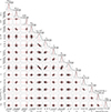 |
Fig. E.1. Posterior distributions of the model fit parameters for Abell 1689. The convention is identical to Fig. C.1. |
Appendix F: Subaru data processing
The image processing for the wide-field imaging in the B, V, RC, i+, and z+ bands, obtained with Suprime-Cam on the 8.2 m Subaru Telescope builds on the AstrOmati software suite2. In particular, the astrometric solution is based on scamp (Bertin 2006, 2010) using Abell 1689 exposures but also archival images taken during the same observing run, with a sliding window of several days around the exposures of interest so that at least 3 exposures constitute the same astrometric instrument. The typical internal accuracy is of order 0.015″ based on using the Two Micron All Sky Survey as reference (2MASS, Skrutskie et al. 2006). SWarp is used for image coaddition (Bertin et al. 2002) after the exclusion of nonphotometric exposures and those collected in poor seeing conditions. We build a model of the PSF and its spatial variations with PSFEx (Bertin 2011) for all the exposures in all the bands. A PSF model is also built on the coadded frames. The recovered PSF Full Width at Half Maximum (FWHM) is found to be  ,
,  ,
,  ,
,  ,
,  , in the B, V, RC, i+, and z+ bands, respectively. Galaxy shapes were measured from the RC-band data, which provide the highest image quality within the dataset in terms of depth and seeing. Source ellipticities were measured using the model-fitting capabilities of SExtractor, assuming the surface brightness distribution of galaxies can be well approximated by a single Sersic profile. The accuracy of this shape measurement technique was extensively assessed in the GREAT3 challenge as part of the Amalgam team (Mandelbaum et al. 2015) and further explored in the context of the preparation of the Euclid mission (Euclid Collaboration: Martinet et al. 2019). Residual multiplicative and additive biases are expected to be well below the statistical uncertainties for the WL signal expected from this cluster.
Photometric redshifts (photo-z) for individual galaxies were estimated by matching the Subaru BVRCi+z+ photometry to the 30-band photometric redshift (photo-z) catalog of the 2 square degree COSMOS field (Laigle et al. 2016). We first degrade the COSMOS2015 photometry when necessary to match the depth of our Abell 1689 data by adding extra noise in the COSMOS2015 catalogue. Then, nearest neighbors in the matched BVRCi+z+ magnitude space are used for each source in order to build a photometric redshift distribution based on 100 nearest neighbors using a fast kd-tree structure (Kennel 2004). The resulting mean, median and dispersion redshift are obtained along with a marginalized mean and standard deviation of the distance ratio β ≡ DLS/DS.
Appendix G: Comparison with ICM thermodynamic profiles from K24
A comparison of the thermodynamic profiles from our analysis with those from K24 is shown in Figure G.1.
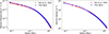 |
Fig. G.1. Electron density (left) and electron pressure (right) profiles generated from the accepted MCMC samples for the fit performed in this work (blue) and K24 (red). |
All Tables
All Figures
|
Fig. 1. Sample mock dataset generated from the smooth models outlined in Section 2. The SZ and X-ray observations were convolved with the Planck/ACT and XMM-Newton beams, respectively, and Gaussian sampled noise was applied to each map. The gray areas on the maps were excluded from the fits (see Section 5). |
| In the text | |
|
Fig. 2. Posterior distribution of M200c and c200c obtained from fits to mock observations. The shaded region for each posterior represents the 68% credible region. The cross indicate the input M200c and c200c used to generate the mock data. The shaded region that matches each cross in color corresponds to the posterior recovered from the mock data generated with that parameter pair. |
| In the text | |
|
Fig. 3. Radial plots of the nonthermal pressure fraction (Pnt/Ptot) recovered from fits to mock observational data, generated with a range of M200cc200c and ℛLP values. The solid purple line represents the best fit model, and the shaded purple region is the corresponding 68% credible region calculated from the accepted MCMC samples. The dashed blue line is the nonthermal pressure fraction calculated from the input parameters used to generate the corresponding mock data. Shaded gray denotes regions where the mass distribution may not be fully constrained from the observed WL shear signal (see Section 5.2). |
| In the text | |
|
Fig. 4. SZ, X-ray, and WL data for the CHEX-MATE galaxy cluster PSZ2 G313.33+61.13 (Abell 1689). The ACT DR6 Compton-y map (top left), the X-ray SB map (top middle), X-ray SB radial profile (top right), two-component WL shear maps (bottom left and middle), and radial profile of X-ray temperature are shown. The grayed-out portions of the maps are data that were excluded from the fit. Bright point-like sources in the X-ray map are indicated by white circles. For the SZ and X-ray portion of the analysis, the data is limited to within the value of R500c obtained by Planck Collaboration XXVII (2016), equal to 7.42′ (1.37 Mpc). The X-ray SB employs a one-dimensional and two-dimensional approach. We use the two-dimensional data within the circular region that encloses 80% of the emission and one-dimensional data is used in the radial region outside of this. For the WL shear maps, we excluded data within 300 h−1 kpc comoving (∼360 kpc physical) to avoid regions containing SL features and significant contamination from cluster member galaxies. |
| In the text | |
|
Fig. 5. Radial profiles of the model SZ (top left), X-ray SB (top right), X-ray temperature (bottom left), and tangential shear (bottom right) obtained from the accepted samples from the MCMC fit to Abell 1689. The dashed vertical black line on the X-ray SB profile indicates the radius at which the two-dimensional analysis (left) transitioned to a one-dimensional analysis (right). The radial profiles of the corresponding observational data are plotted alongside the models. The SZ and X-ray SB model profiles show close agreement to the observational data, so a ratio of the model to the observed data points is shown in the bottom portion of these plots. The profiles of the ICM observables are truncated at the value of R500c obtained by Planck Collaboration XXVII (2016), while the tangential shear extends past this. |
| In the text | |
|
Fig. 6. Posterior distributions of the mass and concentration obtained for a fit to Abell 1689 using SZ, X-ray SB, and temperature, and WL data assuming a triaxial geometry (in green, labeled M200c, triax and c200c, triax) and using only WL data, assuming a spherical geometry (in purple, labeled M200c, sph and c200c, sph). The 68% credible regions for the two results are color-filled in the bottom left subplot. The log normal prior we applied to c200c, which depends on mass, is marginalized over the 68% credible bounds of M200c, triax and plotted in blue in the lower right subplot. Note that the prior is strongly informative and the upper edges of the posterior distributions for c200c are largely set by it. |
| In the text | |
|
Fig. 7. Nonthermal pressure fraction (Pnt/Ptot) from our fit to Abell 1689, along with the corresponding 68% credible region (shaded purple), calculated from the accepted MCMC samples as outlined in Section 3. For comparison, the Pnt/Ptot result obtained for the same cluster by Chappuis et al. (2025) is shown in blue, also plotted with the corresponding 68% credible region. The results in yellow and green show the ensemble-average Pnt/Ptot result from independent analyses of simulated clusters from The300 (Sayers et al. 2021) and Omega500 (Nelson et al. 2014) simulations. The shaded hashed regions for these correspond to the 68% intrinsic cluster-to-cluster scatter within those simulations. Shaded gray denotes regions where the mass distribution may not be fully constrained from the observed WL shear signal (see Section 5.2). |
| In the text | |
|
Fig. 8. Gas-mass fraction computed from our fits to the gas and total mass density (in blue) compared to the ensemble average profile obtained from simulated galaxy clusters from The300 (in pink) used in the analysis of Rasia et al. (2025). The 68% credible region and intrinsic scatter are shown in the shaded region of the respective profiles. We also show a matched sample of five simulated galaxy clusters used in the analysis of Rasia et al. (2025) that have a similar mass and concentration relation to Abell 1689 as dashed purple lines. Additionally, we compared to the result from Eckert et al. (2019), who provide the median value of the gas-mass fraction obtained from a sample of 12 observed galaxy clusters at R500c. Shaded gray denotes regions where the mass distribution may not be fully constrained from the observed WL shear signal (see Section 5.2). |
| In the text | |
|
Fig. A.1. The function used to reconstruct a smooth, conditioned SZ ACT DR6 covariance matrix is shown in purple. It is constructed from an exponential fit (green dashed line) to the inner most black data points and a gaussian fit (red dashed line) to the outer black data points. The black data points were obtained by taking the average of the two-dimensional (unconditioned) covariance matrix in annular bins. |
| In the text | |
|
Fig. C.1. Posterior distributions estimated from our MCMC for a mock observation generated from a smooth model. The green vertical lines in each plot indicate the input parameters used to generate the mock observation maps and the red vertical lines represent the median value from the accepted MCMC samples. The value displayed above each histogram shows the median of the distribution, along with the 1σ (68%) credible region, which is indicated by the dashed vertical lines in every plot. The black line in the two-dimensional distributions encloses the 68% credible region. |
| In the text | |
|
Fig. E.1. Posterior distributions of the model fit parameters for Abell 1689. The convention is identical to Fig. C.1. |
| In the text | |
|
Fig. G.1. Electron density (left) and electron pressure (right) profiles generated from the accepted MCMC samples for the fit performed in this work (blue) and K24 (red). |
| In the text | |
Current usage metrics show cumulative count of Article Views (full-text article views including HTML views, PDF and ePub downloads, according to the available data) and Abstracts Views on Vision4Press platform.
Data correspond to usage on the plateform after 2015. The current usage metrics is available 48-96 hours after online publication and is updated daily on week days.
Initial download of the metrics may take a while.