


| Issue |
A&A
Volume 709, May 2026
|
|
|---|---|---|
| Article Number | A281 | |
| Number of page(s) | 16 | |
| Section | Astrophysical processes | |
| DOI | https://doi.org/10.1051/0004-6361/202659120 | |
| Published online | 27 May 2026 | |
Unveiling hidden millihertz quasi-periodic oscillations in 1A 0535+262
1
Key Laboratory for Particle Astrophysics, Institute of High Energy Physics, Chinese Academy of Sciences, 19B Yuquan Road, Beijing 100049, China
2
School of Physics and Astronomy, University of Southampton, Highfield, Southampton SO17 1BJ, UK
3
Kapteyn Astronomical Institute, University of Groningen, PO BOX 800, NL-9700 AV, Groningen, the Netherlands
★ Corresponding authors: This email address is being protected from spambots. You need JavaScript enabled to view it.
; This email address is being protected from spambots. You need JavaScript enabled to view it.
Received:
25
January
2026
Accepted:
16
April
2026
Abstract
Context. Be/X-ray binary pulsars exhibit transient outbursts and complex timing behaviour, including millihertz quasi-periodic oscillations (QPOs), whose physical origin and energy dependence remain poorly understood. The bright outbursts of 1A 0535+262 in November 2020 provide an ideal laboratory to investigate these properties.
Aims. We aim to characterise the temporal evolution and energy-dependent properties of the millihertz QPO during its 2020 giant outburst, with a focus on trying to detect this feature at lower energies.
Methods. We used the multi-Lorentzian fitting framework that was recently introduced to jointly model the power spectra and the real and imaginary parts of the cross-spectrum. Our analysis incorporates simultaneous broadband X-ray observations from the Neutron Star Interior Composition Explorer (NICER) and Insight-HXMT, spanning the 0.2–120 keV energy range.
Results. We report the first detection of weak, but significant, millihertz QPOs at low X-ray energies (< 27 keV), extending their detection to a new energy regime. The centroid frequency evolves from 41 to 93 mHz, with the peak root-mean-square amplitude detected in the 50–65 keV range. Throughout the outburst, the QPOs generally exhibit a hard lag between 0.12π rad and 0.9π rad. However, at the outburst peak, the higher-energy bands (> 35 keV) display a soft lag of up to ∼ − 0.93π rad. We propose that interactions between soft seed photons and an extended outflow located outside the magnetosphere can account for the observed hard lags, although the physical origin of the transient soft lags remains uncertain. Furthermore, we detect a double-peaked millihertz QPO only at high energies (E > 35 keV) near peak luminosity. The two peaks maintain an approximately constant separation of 2νspin and exhibit anti-correlated phase evolution. The combination of this constant frequency separation and opposite phase trends is difficult to reconcile within existing theoretical models.
Conclusions. Our results indicate that the millihertz QPOs in the Be/X-ray binary 1A 0535+262 are closely linked to the coupled evolution of a soft-photon source and a Comptonising outflow or corona. The joint cross-spectral framework provides a complementary probe of millihertz QPOs beyond traditional power-spectral analyses.
Key words: stars: neutron / X-rays: binaries / X-rays: individuals: 1A 0535+262
© The Authors 2026
 Open Access article, published by EDP Sciences, under the terms of the Creative Commons Attribution License (https://creativecommons.org/licenses/by/4.0), which permits unrestricted use, distribution, and reproduction in any medium, provided the original work is properly cited.
This article is published in open access under the Subscribe to Open model. This email address is being protected from spambots. You need JavaScript enabled to view it. to support open access publication.
1. Introduction
Be/X-ray binaries (BeXRBs) are a subclass of high-mass X-ray binaries (XRBs); they consist of a neutron star (NS) and a Be-type stellar companion. The Be star is typically a rapidly rotating main-sequence or giant star (Reig 2011; Rivinius et al. 2013) surrounded by a quasi-Keplerian circumstellar disc, which forms through episodic mass ejections from the stellar equator. This disc plays a key role in enabling mass transfer onto the NS and strongly influences the system’s X-ray variability (Okazaki et al. 2013; Reig 2007).
Most BeXRBs are transient systems that undergo episodic X-ray outbursts, classified into two types: type I (normal) and type II (giant; Finger et al. 1996a; Bildsten et al. 1997; Negueruela et al. 2001). Type I outbursts are typically periodic, occurring near the periastron passage, and last for a small fraction of the orbital cycle (∼0.2–0.3), with peak luminosities ≲1037 erg s−1. Type II outbursts are more luminous (≳1038 erg s−1), significantly longer in duration, and do not correlate with a specific orbital phase (Frank et al. 2002; Wilson et al. 2008). These giant outbursts are often associated with the temporary formation of an accretion disc around the NS.
During type II outbursts, BeXRBs frequently exhibit strong aperiodic flux variability. Millihertz quasi-periodic oscillations (QPOs) in the ∼1–400 mHz range have drawn particular attention (Bozzo et al. 2009; Boroson et al. 2000). These QPOs are believed to originate from the inner regions of the accretion flow and serve as important diagnostics of accretion dynamics in strongly magnetised NS systems (Dugair et al. 2013; Nandi et al. 2012). Millihertz QPOs have been observed in a variety of sources (e.g. Mukerjee et al. 2001; Revnivtsev et al. 2001; Devasia et al. 2011; Lyu et al. 2016; Bult 2017), and several models have been proposed, such as the beat-frequency (BF) model (Alpar & Shaham 1985), the Keplerian-frequency (KF) model (van der Klis et al. 1987), and NS and disc-precession models (Stella & Vietri 1998). The physical origin of these QPOs, however, remains poorly understood.
Variability in XRBs can be analysed through the power spectrum (PS), which reveals QPOs as narrow features in the Fourier domain (van der Klis 1989; Nowak 2000). However, weak or blended QPO components can remain undetected in the PS, particularly when they coexist with strong broadband noise or overlap with other variability components in the same frequency range (e.g. Zhang et al. 2017, 2020). The cross-spectrum (CS) is another widely used tool in timing analysis, providing a quantitative measure of the correlation between light curves in two different energy bands (Vaughan & Nowak 1997; Nowak et al. 1999; Uttley et al. 2014). The CS encodes phase lags at each Fourier frequency and, together with the PS, enables the computation of the coherence function, a frequency-dependent measure of the linear correlation between concurrent light curves. When extracting phase lags from the CS it is typically assumed that the variability component of interest dominates both the PS and the CS within the selected frequency range (Belloni et al. 2002; Ingram & Motta 2019; Alabarta et al. 2022). This assumption frequently fails in practice when multiple overlapping components contribute to the variability, leading to ambiguous or inaccurate lag estimates (Wang et al. 2021, 2022).
To overcome these limitations, Méndez et al. (2024) introduced a new method that simultaneously fits the PS and the real and imaginary parts of the CS using a multi-Lorentzian model. In this framework, each variability component is described by a Lorentzian profile modulated by a phase lag, under the assumption of coherence within each energy band and incoherence among different variability components (Nowak et al. 1999). By jointly modelling all variability components in both the PS and CS, this approach enables the detection of QPO features that would otherwise remain undetectable using the PS alone. This method also yields reliable estimates of phase lag and coherence, even in the presence of strong contamination from other components. This capability is crucial for uncovering weak or complex QPO signals, as reported in black hole XRBs such as MAXI J1820+070 (Méndez et al. 2024), Cyg X-1 (Fogantini et al. 2025), and Swift J1727.8–1613 (Jin et al. 2025).
We extended this method to investigate the NS XRB 1A 0535+262, a transient X-ray pulsar discovered in 1975 using Ariel V (Rosenberg et al. 1975; Coe et al. 1975). This system consists of a NS in a moderately eccentric orbit (e ∼ 0.47) with an orbital period of approximately 111 days and a spin period of ∼103 s (Finger et al. 1996b). Located at a distance of 2.13 kpc (Bailer-Jones et al. 2018), 1A 0535+262 exhibits cyclotron resonance scattering features at 45 keV and 120 keV, which indicate a surface magnetic field strength (B) of ∼4 × 10¹² G (Kendziorra et al. 1994).
Since its discovery, 1A 0535+262 has exhibited numerous outbursts. According to the disc truncation model proposed by Okazaki & Negueruela (2001), the nature of these outbursts depends on the system’s orbital eccentricity and disc dynamics (Haigh et al. 2004; Coe et al. 2006). At least ten have been classified as type II (Camero-Arranz et al. 2012), during which broad QPOs in the 27–95 mHz range were observed, notably in 1994, 2009, and 2020 (Finger et al. 1996b; Camero-Arranz et al. 2012; Ma et al. 2022).
Interestingly, these millihertz QPOs have consistently been detected only at relatively high energies. Camero-Arranz et al. (2012) found that the QPO amplitude increases with photon energy and becomes undetectable below 25 keV, challenging the explanation of classical BF and KF models. Ma et al. (2022) used broadband observations from Insight-Hard X-ray Modulation Telescope (Insight-HXMT) and detected QPOs up to 80 keV, with the strongest significance in the 50–65 keV range. However, no QPOs were detected below 27 keV, and the observed energy dependence of the root-mean-square (rms) amplitude appeared inconsistent with current theoretical models.
The absence of low-energy X-ray detections leaves the origin of millihertz QPOs unclear, highlighting the need to reassess their behaviour in low-energy bands using the new methodology. In this study, we focused on the 2020 giant outburst of 1A 0535+262, the brightest recorded to date; it reached a peak flux of approximately 11 Crab in the Swift/Burst Alert Telescope (BAT) band (Mandal et al. 2020; Pal & Mandal 2020). The 2020 outburst presents a unique opportunity to explore the characteristics of millihertz QPOs across a broad energy band, as it was observed with high statistical quality by both Insight-HXMT (1–250 keV, 1910 ks) and the Neutron Star Interior Composition Explorer (NICER; 0.2–12 keV, 1900 ks).
We applied the new timing analysis method developed by Méndez et al. (2024) to joint Insight-HXMT and NICER observations of the 2020 outburst of 1A 0535+262, aiming to investigate the broadband (0.2–120 keV) characteristics of the detected millihertz QPO, with particular emphasis on its low-energy behaviour. Section 2 describes the joint fitting model we used. Section 3 outlines the observations and data reduction procedures, and Sect. 4 presents the main results. In Sect. 5 we discuss the implications of our findings, and Sect. 6 summarises our conclusions.
2. Mathematical formalism
We investigated the variability properties of 1A 0535+262 using the new timing method proposed by Méndez et al. (2024), which fits the PS and both the real and imaginary parts of the CS simultaneously. This method enhances the detection of weak or hidden variability components that may not appear significantly in the PS alone but can be recovered through their coherence or phase-lag signatures.
Let x(t) and y(t) denote two simultaneous light curves extracted from different energy bands. Their Fourier transforms are given by X(ν) and Y(ν), and the corresponding PSs are defined as
 (1)
(1)
where ⟨ ⋅ ⟩ indicates averaging over data segments. The complex CS is
 (2)
(2)
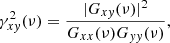
where Δϕxy(ν) is the phase lag between x(t) and y(t) at frequency ν. The intrinsic coherence function is defined as
 (3)
(3)
which quantifies the degree of linear correlation between the signals in different energy bands at each frequency (Vaughan & Nowak 1997; Uttley et al. 2014).
Our joint-fitting approach relies on four assumptions:
-
(i) The variability can be described as a linear combination of Lorentzian components, as commonly adopted in X-ray timing studies (e.g. Nowak 2000; Belloni et al. 2002).
-
(ii) For each Lorentzian component, the centroid frequency ν0, i and width Δi are assumed to be identical in all energy bands, such that the profile of the i-th component is energy-independent (Méndez et al. 2024).
-
(iii) Each Lorentzian component is assumed to be perfectly coherent between any two energy bands.
-
(iv) Any two Lorentzian components that partially overlap in frequency are assumed to be mutually incoherent. This is a widely adopted assumption in modelling NS PSs using multiple (approximately) independent Lorentzian components (e.g. van Straaten et al. 2002).
Following assumption (i), we modelled both PSs as a sum of n Lorentzian functions:
 (4)
(4)
where Ai and Bi are the integrated powers in each band, and L(ν; ν0, i, Δi) denotes the normalised Lorentzian profile; per assumption (ii), the same ν0, i and Δi are used for a given Lorentzian in all energy bands. Following assumption (iii), each Lorentzian is fully coherent between bands x and y (i.e. γxy, i2 = 1), so the variability in bands x and y is related by a deterministic linear transfer, and the CS of the i-th component satisfies
 (5)
(5)
From the above, and using assumption (iv), the total CS is expressed as
 (6)
(6)
where  and Δϕxy, i is the phase lag of the i-th component. In this work, we adopted the constant phase-lag model (see Méndez et al. 2024 for details), where
 (7)
(7)
The real and imaginary parts of the CS are then given as
![Mathematical equation: $$ \begin{aligned} \text{ Re}[G_{xy}(\nu )] = \sum _{i = 1}^n C_i L(\nu ; \nu _{0,i}, \Delta _i) \cos (2{\pi } k_i) \end{aligned} $$](/articles/aa/full_html/2026/05/aa59120-26/aa59120-26-eq9.gif) (8)
(8)
![Mathematical equation: $$ \begin{aligned} \text{ Im}[G_{xy}(\nu )] = \sum _{i = 1}^n C_i L(\nu ; \nu _{0,i}, \Delta _i) \sin (2{\pi } k_i). \end{aligned} $$](/articles/aa/full_html/2026/05/aa59120-26/aa59120-26-eq10.gif) (9)
(9)
The total, frequency-dependent phase lag is reconstructed as
 (10)
(10)
For clarity, we use Δϕxy(ν) to refer to the total observed phase-lag, while ΔϕQPO denotes the intrinsic phase lag of an individual QPO component.
The statistical uncertainty of the squared coherence function is given by (Bendat & Piersol 2011; Vaughan & Nowak 1997):
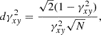 (11)
(11)
where N is the number of averaged segments. This relation shows that the coherence function is substantially more robust to statistical noise than either the PS or CS, especially when γxy2 ≈ 1. Consequently, components with high intrinsic coherence achieve a higher effective signal-to-noise ratio in the coherence spectrum than in the PS or CS, making coherence-based diagnostics particularly powerful for detecting weak but correlated variability (Fogantini et al. 2025; Rout et al. 2025). This effect is especially important in broadband-dominated or high-energy regimes, where background noise often suppresses individual spectral features. The joint modelling of PS and CS not only improves the sensitivity to such weak components but also enables a more comprehensive characterisation of their spectral–timing properties, including their energy-dependent coherence and phase-lag behaviour.
3. Observations and data analysis
3.1. Data reduction
3.1.1. Insight-HXMT
Insight-HXMT (hereafter HXMT) provides broadband X-ray coverage from 1 to 250 keV through three onboard instruments: the Low-Energy X-ray Telescope (LE; 1–10 keV, with an effective area of 384 cm2; Chen et al. 2020), the Medium-Energy X-ray Telescope (ME; 8–35 keV, 952 cm2; Cao et al. 2020), and the High-Energy X-ray Telescope (HE; 27–250 keV, 5100 cm2; Liu et al. 2020).
HXMT monitored 1A 0535+262 with high cadence and high statistics for nearly 50 days during its 2020 giant outburst, collecting a total exposure of over 2.09 Ms. In this work, we focused on data obtained through the HXMT Core Science Program, spanning the period from 14 November to 24 December 2020 (MJD = modified Julian date: 59167.33–59207.72; ObsID P0314316001–P0314316015). Each exposure ID (ExpID) typically provides a long integration time, ranging from 90 to 190 ks.
Furthermore, to improve the signal-to-noise ratio, data products from all ExpIDs observed on the same day, typically 5 to 8 per day, were merged into a single daily dataset. The reorganised datasets used in this analysis are summarised in Table C.1. HXMT data reduction was carried out using HXMTDAS v2.04. Background estimation for the HE, ME, and LE instruments was performed using the corresponding tools–HEBKGMAP, MEBKGMAP, and LEBKGMAP–based on the HXMT background models (Guo et al. 2020; Liao et al. 2020a,b).
3.1.2. NICER
To explore data in the lower energy band, we incorporated observations from NICER (Gendreau et al. 2016), mounted on the International Space Station. NICER is well suited for this purpose due to its lower energy coverage (0.2–12 keV) and large effective area (≥2000 cm2). The NICER observations of 1A 0535+262 span from 11 November 2020 (MJD 59160.23) to 25 February 2021 (MJD 59263.01).
Data reduction was carried out using HEASoft v6.31.1 and the NICERDAS pipeline (version 2022-12-16 V010a), along with the latest calibration files (CALDB vxti20221001). Cleaned event files were produced with nicerl2. Since we focused on the bright phase of the outburst, the background contribution was negligible compared to the source count rate and was therefore not taken into account in our analysis.
The NICER and HXMT light curves of the 2020 outburst of 1A 0535+262 are presented in Fig. 1. The shaded regions indicate the observation periods analysed in this study; detailed information corresponding to these intervals is provided in Table C.1.
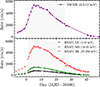 |
Fig. 1. Long-term X-ray light curves of the 2020 outburst of 1A 0535+262. Top panel: NICER count rate in the 0.2–12 keV band. Each observation is represented by a purple square. Bottom panel: HXMT light curves from the Core Science Program (P0314316). The LE (1–10 keV), ME (10–35 keV), and HE (27–250 keV) count rates are represented by the black (bottom), green (middle), and red (top) triangles, respectively. Additional observations from proposal P0304099 (PI: P. Reig) are marked with circles. Each data point represents a single observational epoch. The shaded grey region denotes the interval during which the millihertz QPO was most significantly detected at energies above 27 keV (Ma et al. 2022) and selected for cross-spectral analysis. |
3.2. Computation of PS, CS, coherence, and phase lag
To compute the PS, we employed the GHATS1 software to perform fast Fourier transform using a segment length of 393.216 seconds and a time resolution of 6 ms. The adopted Δt places the HXMT/LE, ME, and HE light curves on a common time grid for the cross-correlation analysis, while the chosen segment length of 393.216 s (i.e. 216 time bins at 6 ms resolution) preserves the low-frequency resolution required for the millihertz-QPO analysis. This configuration yields a minimum frequency (and frequency resolution) of 0.002543 Hz, and a Nyquist frequency of 83 Hz. The light curves were not background-subtracted prior to the Fourier analysis; instead, we accounted for the background statistically in the fractional-rms normalisation of the PSs, which mitigates the dilution of intrinsic variability by background counts, particularly at high HXMT energies (Belloni & Hasinger 1990). To account for the Poisson noise, we subtracted its level from the 60–80 Hz band. We then logarithmically re-binned the PS, increasing the bin width by a factor of ≈1.047 (101/50) for each successive bin. To study the energy dependence of the variability, we divided the NICER data into four energy sub-bands: 0.2–2, 2–5, 5–8, and 8–12 keV. For the HXMT data, we adopted ten sub-bands (see also Ma et al. 2022): 1–3, 3–5, and 5–10 keV for LE, 10–35 keV for ME, and 27–35, 35–40, 40–50, 50–65, 65–80, and 80–120 keV for HE.
The CS was computed using the same segment length and time resolution as the PS. We selected the 0.2–2 keV band as the reference band for NICER, and the 1–3 keV energy band for HXMT data. The corresponding reference and subject bands are listed in Table 1. To correct for the partial correlation of photons present simultaneously in narrow and broad energy bands, we subtracted the average real part of the CS over the same 60–80 Hz range used for noise correction in the PS (Méndez et al. 2024; Bellavita et al. 2025). Phase lags and coherence were derived from the PS and CS (see Sect. 2 and Méndez et al. 2024 for further details). We found that in most observations, the phase lags remain close to zero across a broad frequency range, implying that the imaginary part of the CS is substantially smaller than the real part. To improve the robustness of the model fitting, we applied a 45° rotation to the cross vectors of the two energy bands in the Fourier plane. This transformation equalises the contributions of the real and imaginary components without altering the best-fitting parameters (see Méndez et al. 2024).
Energy bands for cross-spectral analysis.
3.3. Joint fitting model
To independently measure each variability component, we fitted the PS in two bands, Gxx(ν) and Gyy(ν), as well as the real and imaginary parts of the CS, Re[Gxy(ν)] and Im[Gxy(ν)] (for more details, see Sect. 2 and Méndez et al. 2024). Since both the phase lag, Δϕ(ν), and coherence γxy(ν) can be derived from the above four independent spectra, we have flexibility in selecting a subset of four out of the six available spectra for joint modelling (Fogantini et al. 2025; Rout et al. 2025). In our analysis, we chose to fit Gyy(ν) (subject band PS), Re[Gxy(ν)], Im[Gxy(ν)], and γxy(ν). This selection was motivated by the observation that γxy(ν) exhibits prominent structure in our dataset, and it serves as a sensitive diagnostic, especially for identifying variability components that exhibit weaker PS and/or CS. For the MJD 59167 observation, we utilised the phase-lag spectra instead of the coherence spectra, as the latter were of insufficient quality for this dataset; the same choice was adopted for all subject bands with E > 80 keV.
We performed the joint fit using XSPEC v12.14.0h over the 0.02–10 Hz frequency range. During the fitting process, the centroid frequencies (ν0) and full width at half maximum (Δ) of the Lorentzians were linked across the spectra but allowed to vary freely, while the normalisations in the PS and CS were allowed to vary independently. Parameter uncertainties were estimated in XSPEC using the error command with Δχ2 = 2.706, corresponding to the 90% confidence interval for one parameter of interest. Following Méndez et al. (2024), a Lorentzian is considered significant if the normalisation of that component in any of the PS, or the corresponding quantity in the CS, divided by its negative 1σ error, exceeds 3. A component is retained in the joint-fitting model if it is significant in at least one PS or in the CS. From the best-fit model, both the PS of the reference band and the phase lags were derived2.
4. Results
4.1. Hidden millihertz QPOs in the low-energy band
We first analysed the coherence and phase lags across all HXMT observations, with emphasis on the low-energy band (< 27 keV). In 1A 0535+262, during the outburst peak (MJD 59167–59194, Days 1–28; ObsID P0314316001–P0314316011), the coherence shows a marked decrease and the phase lags exhibit a pronounced feature at the QPO frequencies identified in the high-energy PS (Fig. B.1), spanning the full energy range. As noted in Appendix A, similar features appear in some HXMT/LE data but at lower significance than in HXMT/ME and HE data; during the rise and decay phases of the outburst, limited statistics preclude a firm confirmation of such structures. Similar behaviour has been reported in several black hole XRBs (e.g. MAXI J1820+070, Bellavita et al. 2025; Cyg X-1, Fogantini et al. 2025; and Swift J1727.8–1613, Jin et al. 2025), and has been attributed to the presence of a hidden QPO-like component.
To verify the characteristics of the coherence and phase lags, particularly in the low-energy band, we analysed the set of NICER data, taking advantage of its larger effective area compared with HXMT/LE. The NICER observations reproduce the main features seen in the HXMT data, especially during the outburst peak (MJD 59167–59191, Days 1–25; ObsID 3200360130–3200360152).
Given NICER’s higher statistical quality (clearer structure in coherence and phase lags) and better low-energy coverage, we used NICER data (0.2–12 keV) in place of the HXMT/LE data (1–10 keV); for the high-energy band, we continued to use HXMT/ME and HE data (10–120 keV). To quantitatively characterise the structures in the coherence and phase-lag spectra and explore the low-energy properties of 1A 0535+262, we applied the joint fitting method proposed by Méndez et al. (2024, see also Sect. 3.3 in this work).
We present representative low-energy fitting results using NICER data in Fig. 2, including the PS of the reference (0.2–2 keV) and subject (8–12 keV) bands, the real and imaginary parts of the CS (after a 45° rotation), the coherence, and the phase-lag spectra. The data are described well by a model with five Lorentzian components, yielding χ2 = 403.92 for 399 degrees of freedom (d.o.f.) One of these Lorentzians, centred at 61.9 ± 4 mHz (vertical dash-dot line), represents an additional feature not identifiable from the PS alone. To check its robustness, we repeated the fitting without this extra component. In the coherence and phase-lag panels, the model derived from this reduced fit (dashed curves) leaves systematic residuals: it fails to reproduce the observed coherence dip at ∼62 mHz and the associated bump in the phase-lag spectrum. This demonstrates that the additional Lorentzian is required by the data, with a detection significance of 3.2σ in the joint-fit model. The centroid frequency of this feature is consistent with the QPO frequency measured in the high-energy PS (see below). At the same frequency, the coherence drops sharply from ∼0.9 to ∼0.2, accompanied by a bump-like feature in the phase-lag spectrum peaking at ∼0.4 rad. Although this variable component does not produce a distinct peak in the PS at low energies, the corresponding structure in the coherence and phase lag provides strong evidence of an underlying variability component analogous to the millihertz QPOs observed at higher energies. We therefore suggest this feature is the ‘hidden’ millihertz QPO: a component not directly visible in the PS, but required to reproduce the observed coherence and phase-lag behaviour.
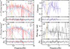 |
Fig. 2. Joint fit to the NICER data of 1A 0535+262 from Day 1. (a) PS of the reference (0.2–2 keV; blue) and subject (8–12 keV; red) bands. (b) 45°-rotated CS: Rerot (blue) and Imrot (red; QPO Rerot sign-flipped; see Fig. A.2a). In (a) and (b), solid and dashed curves show the total five-Lorentzian model and individual components. (c) Coherence and (d) phase lags, with models including (solid) and excluding (dashed) the QPO. Dash-dotted yellow line marks the QPO centroid frequency, which coincides with a coherence dip and phase-lag rise. Data above ∼1 Hz are logarithmically re-binned with a factor of exp(1/10). Bottom sub-panels: Residuals, Δχ = (data − model)/error. |
When the subject band is HXMT/HE (50–65 keV), the PS of the hard band exhibits a prominent and narrow QPO peak, as reported in Ma et al. (2022). An illustrative fit is shown in Fig. 3. At the QPO centroid frequency, the phase-lag spectrum displays a steep rise (the ‘phase-lag cliff’), while the coherence function shows a localised dip, consistent with the behaviour observed in the lower-energy bands. For comparison, we also computed model predictions after removing the QPO component from the fit. In this case, the model failed to reproduce the PS in the 50–65 keV, confirming the 12.4σ detection significance of the QPO component. The corresponding coherence and lag curves are shown as dashed lines in Fig. 3. At low frequencies (f ≲ 0.2 Hz), the coherence remains low (≲0.4) and is only weakly affected. In contrast, the phase-lag spectrum becomes nearly flat, failing to reproduce the upturn observed at the QPO frequency. These results further indicate that the QPO properties hidden in the lower-energy bands are essentially the same as those observed in the high-energy bands.
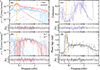 |
Fig. 3. Same layout as Fig. 2 but for HXMT data. The reference and subject bands are 1–3 and 50–65 keV, respectively. Negative Lorentzian contributions to Rerot or Imrot are plotted with reversed signs; see Fig. A.2b. |
4.2. Energy dependence of millihertz QPOs
Figure 4 presents the energy-dependent evolution of the QPO properties, including fractional rms amplitude and phase lag (ΔϕQPO), across three representative epochs corresponding to the rise, peak, and decay phases of the outburst. The rms amplitude exhibits a pronounced energy dependence. In the low-energy band (< 12 keV), the fractional rms remains below ∼5%. Above this energy, the amplitude rises with energy, peaking at ∼15–18% around 60 keV, and subsequently decreases to ∼6% at higher energies.
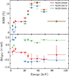 |
Fig. 4. Energy dependence of the millihertz QPO properties in 1A 0535+262 for three epochs (MJD 59169, 59172, and 59181; corresponding to Days 3, 6, and 15). Top panel: Fractional rms amplitude as a function of energy. Bottom panel: Energy-resolved phase lag, ΔϕQPO, measured with respect to the reference band. Triangles and squares denote HXMT and NICER measurements, respectively. Colours indicate the outburst phase: red (rise), blue (peak), and green (decay). In each energy band, the QPO was modelled with a single Lorentzian component. |
The phase lag, ΔϕQPO (Fig. 4, right panel), shows a pronounced and phase-dependent evolution with energy. At soft X-ray energies (≲12 keV), the lag differs markedly between epochs: it is close to zero on Day 3 (MJD 59169; ∼0.03π rad–0.22π rad), remains around ∼0.4π rad on Day 13 (MJD 59181), and reaches the largest values on Day 6 (MJD 59172; ∼0.84π rad–0.98π rad). With increasing energy, Day 3 stays near zero up to ∼31 keV, then turns negative and reaches a minimum of ∼ − 0.46π rad at ∼72.5 keV, followed by a partial recovery to ∼ − 0.17π rad at ∼100 keV (with larger uncertainties at the highest energies). On Day 6, the lag drops rapidly from ∼π rad at ≲12 keV to negative values, reaching ∼ − 0.64π rad at ∼35–40 keV and remaining at ∼ − 0.5π rad above ∼70 keV. In contrast, Day 13 stays positive across the full band, peaking at ∼0.78π rad–0.86π rad around ∼27–40 keV, showing a shallow dip to ∼0.65π rad near ∼60 keV, and stabilising at ∼0.84π rad at higher energies.
4.3. Time evolution of the millihertz QPO
To explore the time-dependent behaviour of the millihertz QPO, we divide the analysis into two energy regimes: soft bands (< 12 keV; shown in bluish tones) and hard bands (> 12 keV; shown in violet hues) in Fig. 5. The left panels show the evolution of the QPO centroid frequency, half-width at half maximum (HWHM), and fractional rms amplitude, while the right panel presents the phase lag, ΔϕQPO, over the outburst.
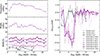 |
Fig. 5. Time evolution of millihertz QPO parameters in 1A 0535+262 during the 2020 outburst. Left three panels: Centroid frequency, HWHM, and rms amplitude of the QPOs as functions of MJD. Right panel: QPO phase lag (ΔϕQPO) for the energy bands listed in the legend, measured relative to 0.2–2 keV for NICER and 1–3 keV for HXMT. NICER data are shown in grey and HXMT data in violet. The QPO signal in each energy band was fitted with a single Lorentzian component. |
The QPO centroid frequency rises rapidly from ∼62 mHz to a maximum of ∼91 mHz during the early outburst (Days 1–7; MJD 59167–59173), and subsequently decreases gradually to ∼56 mHz in the late decay. This evolution broadly follows the luminosity profile inferred from the X-ray light curve (see also Ma et al. 2022). The HWHM shows moderate fluctuations (typically ∼23–50 mHz) without a clear systematic trend, although it tends to be narrower in the late decay (≲25 mHz). The fractional rms displays a strong energy dependence but only weak temporal variability: it stays at a few per cent in the NICER soft bands and increases to ∼(6–17)% in the HXMT hard bands, with no clear systematic trend with outburst phase.
The phase-lag evolution shows a clear contrast between soft and hard energies (right panel of Fig. 5). In the NICER soft bands (< 12 keV), ΔϕQPO is predominantly positive and is typically around ∼ 0.8π rad during most of the rise and the peak epoch, with a brief drop to values consistent with zero around Day ∼3 and a decrease towards the end of the NICER coverage (down to ≲ 0.5π rad). The HXMT/ME 10–35 keV lag is generally smaller (typically ≲ 0.4π rad) during the rise and peak, but becomes larger in the decay, reaching ∼(0.6–0.7)π rad at late times, albeit with sizeable uncertainties.
In contrast, the HXMT/HE bands exhibit a pronounced sign reversal during the peak epoch. The lags are positive at the onset (Days ∼1–2; ∼(0.6–0.9)π rad), then turn negative during Days ∼3–8, reaching the most negative values around Day ∼7–8 (ranging from ∼ − 0.56π rad to −0.93π rad, depending on energy). After Day ∼9, the lags flip back to positive and remain approximately stable at ∼(0.7–0.8)π rad through the decay, with only modest energy-to-energy scatter.
4.4. The double-peaked QPO profile
During the peak of the outburst, a double-peaked structure appears near the QPO centroid frequency in the high-energy (> 27 keV) PSs. This feature is not significantly detected at lower energies, consistent with the findings of Ma et al. (2022). In this section we re-examine this double-peaked profile and extend the analysis to the associated phase-lag behaviour for two representative epochs, Day 5 and Day 8 (MJD 59171 and 59174).
Figure 6 presents the joint modelling of the PS and the corresponding phase-lag spectra in the HXMT/HE 50–65 keV band for both epochs, using HXMT/LE 1–3 keV as the reference band. We tested two alternative descriptions of the QPO feature: a single-QPO model composed of five Lorentzians (red) and a double-QPO model with six Lorentzians (green), where the additional component accounts for the resolved double peak. To ensure a direct comparison, the frequencies and widths of all non-QPO components were tied between the single- and double-QPO models.
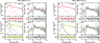 |
Fig. 6. Single- and double-QPO fits to the HXMT/HE 50–65 keV subject band on Day 5 (MJD 59171; panels a–d) and Day 8 (MJD 59174; panels e–h), shown for the PS νPν and the corresponding phase-lag spectrum relative to the HXMT/LE 1–3 keV reference band. Panels (a), (c), (e), and (g): Single-QPO model (five Lorentzians; solid red curves). Panels (b), (d), (f), and (h): Double-QPO model (six Lorentzians; solid green curves). Dashed curves denote individual Lorentzian components; in the double-QPO model, the LF and HF QPO peaks are highlighted with dashed red and blue curves, respectively, consistent with Fig. 7. Residuals (Δχ) are shown beneath each spectrum. |
On Day 5, the single-QPO fit gives νQPO = 86.7 ± 3.1 mHz. In the double-QPO model, this feature is resolved into two components, hereafter referred to as the lower-frequency (LF) and higher-frequency (HF) peaks. Their centroid frequencies are  mHz (QLF ≃ 1.7) and
  mHz (QHF ≃ 7.8), separated by ∼0.02 Hz, where Q ≡ ν/Δ. A similar decomposition is found on Day 8: the single-QPO centroid is
  mHz, whereas the two-component fit yields νLF = 78.0 ± 7.6 mHz (QLF ≃ 2.5) and
 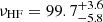 mHz (QHF ≃ 4.3). The implied frequency ratio, νHF/νLF ≈ 1.25, disfavours a harmonic origin (i.e. a 1:2 fundamental-harmonic relationship).
While the two models provide comparable representations of the overall PS, the double-QPO model more accurately reproduces the sharp phase-lag transition at the QPO frequencies, which appears as a narrow, structured feature in the lag spectrum. Importantly, such a two-component description is not required at lower energies for the same epochs. For example, the phase-lag spectra in HXMT/ME 10–35 keV (reference: 1–3 keV) and in NICER 5–8 keV (reference: 0.2–2 keV) are adequately described by a single broad QPO component.
The energy dependence of the two resolved components is summarised in Fig. 7. On Day 5, both LF and HF rms amplitudes show a convex trend with energy, peaking around 50–65 keV, with the HF component generally being stronger. The phase lags are clearly component-dependent: the LF peak remains positive (ranging from ∼ 0.35π rad to 0.71π rad) with only mild energy dependence, whereas the HF peak stays negative and becomes slightly less negative at higher energies (typically between ∼ − 0.76π rad and −0.09π rad). On Day 8, the overall rms level increases, and the LF component becomes dominant above ∼40 keV. Meanwhile, the lag signs reverse: the LF lags become negative (down to ∼ − 0.79π rad), while the HF lags remain mildly positive and nearly energy-independent (∼ 0.24π rad).
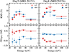 |
Fig. 7. Energy dependence of the double-peak QPO properties in 1A 0535+262 on MJD 59171 and 59174. Top panels: rms amplitude as a function of energy. Bottom panels: Phase lags (ΔϕQPO). The filled blue and open red triangles represent the HF and LF QPOs, respectively. The differences in both rms amplitude (∼4.5% on Day 5 and ∼6.6% on Day 8) and phase lag (∼0.9π rad) remain approximately constant across the 27–120 keV energy range. |
In summary, the double-peaked description is required to reproduce the high-energy lag structure but is not necessary for the contemporaneous lower-energy lag spectra. Moreover, the two resolved peaks exhibit distinct phase lags, yet maintain an approximately constant phase separation of ∼π rad across the hard X-ray band.
5. Discussion
Using high-statistics, broadband (0.2–120 keV) observations from NICER and HXMT, we applied the new analysis technique proposed by Méndez et al. (2024), originally developed for black-hole XRBs and here employed for the first time in a NS XRB. With this new method, we detect 47–98 millihertz QPOs in 1A 0535+262 during its 2020 outburst. While such QPOs had previously been reported only in the hard X-ray band (e.g. Finger et al. 1996b; Camero-Arranz et al. 2012; Ma et al. 2022), our analysis provides the first significant detection of these features in the soft X-ray band, at energies below 27 keV. We further extended the analysis of the double-peaked QPOs observed at the outburst peak (see also Ma et al. 2022) by investigating their phase lags using the same method of Méndez et al. (2024). Across the energy bands, the two QPO components exhibit an almost constant phase-lag offset of ∼1.1π rad. Temporally, their phase evolution is anti-correlated, with the relative offset transitioning from π rad to −π rad around Day 6, indicating a full 2π rad reversal. Finally, we combined the newly uncovered soft X-ray characteristics of the millihertz QPO with insights from the double-peaked structure to explore the possible physical origin of these oscillations.
5.1. Detection of low-energy millihertz QPOs and their physical implications
We find that the millihertz QPO is detected not only in the harder X-ray band (> 27 keV) but also, as a weaker yet significant feature, in the soft band (< 27 keV). This conclusion is supported by the joint PS+CS fitting analysis, in which the inclusion of a QPO component substantially improves the fit to both the coherence and phase-lag spectra, even though no distinct peak is visible in the soft-band PS (see Fig. 2). The coherence shows a localised dip and the phase lag exhibits a bump at the QPO frequency, confirming the presence of a correlated variability component. This demonstrates that the modulation is not confined to the hard X-ray emitting radiation but is also linked to soft-emission components, such as the magnetosphere–inner disc interface.
5.1.1. Review of BF and KF scenarios
Two models are commonly invoked to explain millihertz QPOs in NS XRBs. In the BF model, accretion material at the inner disc edge orbits at the KF and is accreted onto the NS under magnetic control; the stellar magnetic field, rotating at the NS spin frequency, modulates the both accretion rate and luminosity (Alpar & Shaham 1985; Shaham 1987; van der Klis 2006). In the KF model, QPOs arise from partial obscuration by disc inhomogeneities near the inner edge (van der Klis et al. 1987). Earlier non-detections of QPOs below ∼27 keV (e.g. Finger et al. 1996b; Camero-Arranz et al. 2012; Ma et al. 2022) were taken as evidence against both models (Ma et al. 2022). Here, we re-examine these scenarios in light of our new detections of the QPO in the softer X-ray band.
Assuming that the QPO frequency reflects the dynamical timescale at the truncated inner disc, rk(νK) = (GM/4π2νK2)1/3, adopting a canonical NS with M = 1.4 M⊙ and using the spin period of this system Ps ≃ 103 s (νs ≃ 9.7 mHz), the observed QPO centroid frequency νQPO ≃ 41–93 mHz implies, for the KF model (νK = νQPO), rk ≃ (1.41–0.82)×109 cm, and for the BF model (νK = νQPO + νs), rk ≃ (1.22–0.76)×109 cm. To compare with the magnetospheric radius, we computed the standard Alfvén radius,  and set rM = ξrA with ξ ≃ 0.5–1. For 1A 0535+262, using representative parameters, B12 ≃ 4.7, R6 = 1, L37 ≃ 1–12 (Kong et al. 2021), we obtain rM ≃ (0.19–0.78)×109 cm, comparable to the radii inferred from the QPO frequency, rk ≃ (0.76–1.41)×109 cm (KF and BF ranges combined). This is consistent with the interpretation that the millihertz QPO originates from variability at the magnetosphere–disc boundary. Moreover, the observed νQPO–LX relation broadly follows the νQPO ∝ LX3/7 scaling expected in standard BF and/or KF frameworks (Finger et al. 1996b; Ma et al. 2022, for HXMT results in 2020; see Fig. 6 in Ma et al. 2022).
The correlation of QPO frequencies with the inner disc radius, together with the detection of low-energy QPOs, is consistent with both the KF and BF models. However, the rms–energy dependence requires further consideration: the rms of the QPO peaks at intermediate energies (50–65 keV) and decreases towards both the soft (≲27 keV) and hard (≳65 keV) bands. As reported by Ma et al. (2022), this behaviour is not accounted for by either model. The KF model does not predict energy-dependent rms, with the variations arising solely from partial disc obscuration, while the bulk and thermal Comptonisation model of the accretion column (bwcycl; Becker & Wolff 2007; Ferrigno et al. 2009) likewise does not reproduce such an energy dependence (see Ma et al. 2022).
The suppression of rms variability at ≲2–3 keV can be attributed to dilution by stable disc emission (e.g. La Palombara & Mereghetti 2006; Uttley et al. 2014). However, this explanation alone cannot account for the gradual decline extending up to ∼50 keV in 1A 0535+262, where thermal Comptonisation is expected to dominate (e.g. Becker & Wolff 2007; Ferrigno et al. 2009). Moreover, the reduction of rms at higher energies (≳65 keV) cannot be simply explained by photon up-scattering, as this process can enhance the rms in some black-hole XRBs (e.g. Yu et al. 2024). This may indicate that, for the highest-energy photons, the scattering or transfer process becomes less effective at imprinting the QPO modulation, leading to reduced rms. In summary, the observed symmetric rms–energy profile – with a peak at 50–65 keV and a decline towards both lower and higher energies – suggests a more complex origin of the energy-dependent variability than previously thought.
5.1.2. Phase-lag evolution with luminosity and beam geometry
The QPO phase lags in 1A 0535+262 show a strong dependence on both photon energy and source luminosity. In the soft band (E < 27 keV), the lags remain hard, increasing from ∼0.1π rad during the rise to ∼0.9π rad close to the luminosity maximum, and then decreasing to ∼0.4π rad during the decay. Conversely, in the hard band (E ≳ 35 keV) the lag undergoes a transient reversal near the outburst peak, evolving from ∼0.8π rad in the rise to ∼ − (0.8–0.9)π rad at maximum luminosity, before returning to ∼0.7–0.8π rad in the decay. Similar lag reversals have been observed in black-hole binaries (e.g. XTE J1550−564 and GRS 1915+105) and are associated with structural changes in the Comptonising region (Wijnands et al. 1999; Cui et al. 2000; Pahari et al. 2013).
We defined the lag-reversal luminosity as Lrev ≃ (1.11–1.16)×1038 erg s−1 (vertical shaded region in Fig. 8). Below this threshold (L ≲ Lrev), the lags are hard across all bands, typically clustering around 0.6π–0.9π rad, with occasional excursions down to ∼0.1π rad and up to ∼1.1π rad. Within a narrow luminosity interval around the outburst peak, L ≃ (1.16–1.25)×1038 erg s−1, the high-energy lags (E ≳ 35 keV) become negative, reaching ΔϕQPO ≈ −(0.6–0.9)π rad, whereas the low-energy lags remain positive. As the luminosity falls below Lrev, the soft lags disappear and all bands revert to hard lags, demonstrating that the lag behaviour is tightly regulated by luminosity.
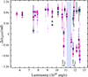 |
Fig. 8. Luminosity–phase–lag relation of the millihertz QPO in 1A 0535+262. ΔϕQPO in different energy bands (colours as in Fig. 5) versus bolometric luminosity. The light blue shaded region indicates the transition range, Lrev ∼ 1.11 − 1.16 × 1038. A transient soft lag appears only for L ≳ Lrev. All QPOs were fitted with a single-component model. |
We first evaluated whether the observed lags could arise from local geometric effects, such as energy-dependent beaming and/or multiple emission components (e.g. hotspots or accretion columns; Caballero et al. 2011; Mushtukov et al. 2018). If these lags were produced locally within the emission region, the intrinsic formation and scattering timescales for soft and hard photons near the surface or column – of the order of ∼10−5 s (Mushtukov et al. 2015) – would be far shorter than the observed seconds-scale time lags. In addition, hard-photon production via bulk Comptonisation within the magnetosphere is unlikely to be efficient given the limited scattering depth (e.g. Becker & Wolff 2007). Moreover, although local radiation patterns can be highly anisotropic (e.g. Poutanen & Gierliński 2003; Poutanen & Beloborodov 2006), viewing-angle effects are typically coupled to the NS spin frequency rather than producing a stable phase offset at the QPO frequency, unless the QPO itself is driven by a unique geometric modulation (e.g. warped jet precession in MAXI J1820+070; Ma et al. 2021). We therefore suggest that local mechanisms can contribute but that they are insufficient to account for the large-amplitude, luminosity-dependent lag evolution.
A stable phase lag at the QPO frequency is more naturally explained if it arises from delays introduced by scattering and/or irradiation and reprocessing between spatially distinct regions (e.g. Kotov et al. 2001; Arévalo & Uttley 2006; Karpouzas et al. 2020). We therefore considered a global scenario in which the lags arise from the coupled variability of the accretion column and an extended hot Comptonising medium outside the magnetosphere (hereafter, the outflow or corona). The measured QPO time lags span approximately −5 s to +8 s. A simple order-of-magnitude estimate based on the light-travel distance, c|Δt|, yields a characteristic scale of ∼(1.5–2.4)×1011 cm, which is orders of magnitude larger than the magnetospheric radius (Rm ∼ 108–109 cm), yet remains below the NS Roche-lobe radius (RL ∼ 1012 cm). Although c|Δt| should be interpreted as an upper limit, the large mismatch between c|Δt| and Rm suggests that the dominant lag-producing region cannot be confined within the magnetosphere. Instead, a more plausible interpretation is that the QPO originates at larger radii in the outer accretion disc, where scattering and irradiation and reprocessing can naturally generate energy-dependent QPO lags.
Within this framework, we propose that the lag evolution is linked to the interaction of soft photons with the outflow or corona. The coupling between the inner disc and the NS magnetic field may drive an extended outflow through magnetic and radiative forces, and dissipation of magnetic energy can maintain a hot, low-density Comptonising medium at large radii (Romanova et al. 2009; Lii et al. 2012). The presence of an outflow is also qualitatively consistent with radio detections (van den Eijnden et al. 2022), which may trace synchrotron emission associated with open field lines and/or out-flowing plasma in the transition region. At L ≲ Lrev, hard lags can be produced if soft seed photons from the inner disc and/or magnetospheric inflow are Compton up-scattered in the hot outflow or corona.
However, the transient soft lags at high luminosity are not straightforward to explain within this picture. One possibility is that near the outburst peak, the outflow becomes increasingly optically thick while remaining hot, shielding a substantial fraction of the soft seed photons. At the same time, hard X-rays from the Comptonising medium may irradiate the disc and/or dense material in the inner flow more efficiently and be reprocessed into softer emission. If this reprocessed component is viewed under a favourable geometry, it may dominate the soft band and thus produce the observed soft lag. The strength of this effect remains uncertain, and a quantitative explanation of the observed soft lags will require further theoretical constraints and more detailed modelling.
5.2. Insight from the double-peaked QPO profile at the outburst peak
During the outburst peak (MJD 59171–59177), we detect a double-peaked millihertz QPO exclusively in the hard energy band (E ≳ 35 keV). This feature is evident not only in the PS (see also Ma et al. 2022), but is further supported by the corresponding lag behaviour. The separation between the centroid frequencies of the two peaks is ≃0.02 Hz, which is consistent with being twice the spin frequency of 1A 0535+262. The double peak appears only at the outburst maximum and is temporally coincident with the soft-lag window, implying that its geometry is luminosity-dependent.
In Sect. 5.1.2 we discuss a scenario where soft seed photons originate near the NS, while hard photons are predominantly produced at larger radii within an extended, hot Comptonising medium created by a strong, magnetically dissipative outflow outside the magnetosphere. At high luminosities, numerical simulations suggest that accretion columns can inflate and transition towards a fan-beam dominated emission pattern (e.g. Zhang et al. 2022; Sheng et al. 2023), which would enhance the irradiation of the disc or outflow. In addition, the accretion flow may undergo a regime transition from radiation-inefficient to radiation-dominated state, further modifying the reprocessing or scattering environment. These structural changes allow a larger fraction of seed photons to be emitted at wider angles, facilitating more efficient illumination of the outflow or corona and boosting the hard-band flux. However, these geometric considerations alone do not account for the observed double-peaked QPO. Although vertically stratified (e.g. Basko & Sunyaev 1976; Becker & Wolff 2007; West et al. 2017) or hollow-column structures (e.g. Zhang et al. 2025) may account for multi-component variability at high luminosities, the fixed frequency separation ≃2νspin and the distinct phase-lag evolution of the two peaks impose strong constraints on such interpretations. Consequently, these localised models appear insufficient to fully reconcile the observed properties of the double-peaked QPO, suggesting that a more complex coupling between the pulsation geometry, the disc, and the global outflow dynamics is required.
6. Conclusions
Based on simultaneous NICER and HXMT observations of the BeXRB 1A 0535+262 in the 0.2–120 keV band during the 2020 giant outburst, we applied the recently proposed combined power and CS multi-Lorentzian fitting method (Méndez et al. 2024) to NS XRBs for the first time, enabling a systematic study and characterisation of the broadband timing properties of millihertz QPOs. Our main conclusions are as follows:
-
We detected 41–93 millihertz QPOs in 1A 0535+262 in the hard X-ray band, as previously reported (Finger et al. 1996b; Camero-Arranz et al. 2012; Ma et al. 2022). We also, for the first time, identified a hidden millihertz QPO in the soft X-ray band (< 27 keV) using the new timing analysis method proposed by Méndez et al. (2024).
-
The QPO centroid frequency correlates positively with luminosity. The QPO rms exhibits a convex dependence on energy, peaking at ∼50–65 keV (∼17%) and decreasing both at lower and higher energies, reaching values as low as ∼4% in the softest band.
-
For luminosities below the lag-reversal threshold (L ≲ Lrev), the QPO shows hard phase lags at all energies, ranging from 0.4π rad to 0.9π rad. Near or above Lrev, the phase lags in the hard band transition to soft lags, reaching ∼ − 0.93π rad, while the soft energies maintain hard lags. Interactions between soft seed photons and a strong, extended outflow can naturally introduce seconds-scale hard lags, whereas the origin of the transient soft lags remains uncertain.
-
In the hard band, we confirm double-peaked QPOs with a constant separation of Δν ≃ 0.02 Hz. The two components exhibit distinct phase lags with opposite signs, maintaining a nearly constant phase separation of ∼π rad. This anti-phase coupling is difficult to reconcile with existing models.
These results highlight the power of energy-resolved, coherence-based timing techniques in revealing weak or hidden variability in accreting X-ray pulsars. However, the origin of millihertz QPOs, especially the double-peaked QPOs, remains uncertain, warranting further theoretical investigation.
Acknowledgments
This work made use of data from the Insight-HXMT mission, a project funded by the China National Space Administration (CNSA) and the Chinese Academy of Sciences (CAS), and of observations from the NICER mission supported by NASA. We sincerely thank Sergey Tsygankov for useful discussions and suggestions. We also thank the referee for the constructive comments that improved the quality of this paper. This work was supported by the National Key R&D Program of China (Grant No. 2021YFA0718500). Additional support was provided by the National Natural Science Foundation of China (Grant Nos. 12122306, 12025301, 12333007, and 12103027), the Strategic Priority Research Program of the Chinese Academy of Sciences, and the China’s Space Origins Exploration Program.
References
- Alabarta, K., Méndez, M., García, F., et al. 2022, MNRAS, 514, 2839 [NASA ADS] [CrossRef] [Google Scholar]
- Alpar, M. A., & Shaham, J. 1985, Nature, 316, 239 [NASA ADS] [CrossRef] [Google Scholar]
- Arévalo, P., & Uttley, P. 2006, MNRAS, 367, 801 [Google Scholar]
- Bailer-Jones, C. A., Rybizki, J., Fouesneau, M., Mantelet, G., & Andrae, R. 2018, AJ, 156, 58 [NASA ADS] [CrossRef] [Google Scholar]
- Basko, M. M., & Sunyaev, R. A. 1976, MNRAS, 175, 395 [Google Scholar]
- Becker, P. A., & Wolff, M. T. 2007, ApJ, 654, 435 [NASA ADS] [CrossRef] [Google Scholar]
- Bellavita, C., Méndez, M., García, F., Ma, R., & König, O. 2025, A&A, 696, A128 [NASA ADS] [CrossRef] [EDP Sciences] [Google Scholar]
- Belloni, T., & Hasinger, G. 1990, A&A, 227, L33 [NASA ADS] [Google Scholar]
- Belloni, T., Psaltis, D., & van der Klis, M. 2002, ApJ, 572, 392 [NASA ADS] [CrossRef] [Google Scholar]
- Bendat, J. S., & Piersol, A. G. 2011, Random Data: Analysis and Measurement Procedures, 4th edn. (Wiley) [Google Scholar]
- Bildsten, L., Chakrabarty, D., Chiu, J., et al. 1997, ApJS, 113, 367 [CrossRef] [Google Scholar]
- Boroson, B., O’Brien, K., Horne, K., et al. 2000, ApJ, 545, 399 [Google Scholar]
- Bozzo, E., Stella, L., Vietri, M., & Ghosh, P. 2009, A&A, 493, 809 [NASA ADS] [CrossRef] [EDP Sciences] [Google Scholar]
- Bult, P. 2017, ApJ, 837, 61 [CrossRef] [Google Scholar]
- Caballero, I., Kraus, U., Santangelo, A., Sasaki, M., & Kretschmar, P. 2011, A&A, 526, A131 [NASA ADS] [CrossRef] [EDP Sciences] [Google Scholar]
- Camero-Arranz, A., Finger, M., Wilson-Hodge, C., et al. 2012, ApJ, 754, 20 [NASA ADS] [CrossRef] [Google Scholar]
- Cao, X., Jiang, W., Meng, B., et al. 2020, Sci. China Phys. Mech. Astron., 63, 249504 [NASA ADS] [CrossRef] [Google Scholar]
- Chen, Y., Cui, W., Li, W., et al. 2020, Sci. China Phys. Mech. Astron., 63, 249505 [NASA ADS] [CrossRef] [Google Scholar]
- Coe, M., Carpenter, G., Engel, A., & Quenby, J. 1975, Nature, 256, 630 [NASA ADS] [CrossRef] [Google Scholar]
- Coe, M. J., Reig, P., McBride, V. A., Galache, J. L., & Fabregat, J. 2006, MNRAS, 368, 447 [Google Scholar]
- Cui, W., Zhang, S. N., & Chen, W. 2000, ApJ, 531, L45 [Google Scholar]
- De Marco, B., Adhikari, T. P., Ponti, G., et al. 2020, A&A, 634, A65 [NASA ADS] [CrossRef] [EDP Sciences] [Google Scholar]
- Devasia, J., James, M., Paul, B., & Indulekha, K. 2011, MNRAS, 417, 348 [Google Scholar]
- Dugair, M. R., Jaisawal, G. K., Naik, S., & Jaaffrey, S. 2013, MNRAS, 434, 2458 [Google Scholar]
- Ferrigno, C., Becker, P. A., Segreto, A., Mineo, T., & Santangelo, A. 2009, A&A, 498, 825 [NASA ADS] [CrossRef] [EDP Sciences] [Google Scholar]
- Finger, M. H., Koh, D. T., Nelson, R. W., et al. 1996a, Nature, 381, 291 [Google Scholar]
- Finger, M. H., Wilson, R. B., & Harmon, B. A. 1996b, ApJ, 459, 288 [NASA ADS] [CrossRef] [Google Scholar]
- Fogantini, F. A., García, F., Méndez, M., König, O., & Wilms, J. 2025, A&A, 696, A237 [NASA ADS] [CrossRef] [EDP Sciences] [Google Scholar]
- Frank, J., King, A., & Raine, D. J. 2002, Accretion Power in Astrophysics, 3rd edn. (Cambridge, UK: Cambridge University Press) [Google Scholar]
- Gendreau, K. C., Arzoumanian, Z., Adkins, P. W., et al. 2016, in Space Telescopes and Instrumentation 2016: Ultraviolet to Gamma Ray, eds. J. W. A. den Herder, T. Takahashi, & M. Bautz, SPIE Conf. Ser., 9905, 99051H [NASA ADS] [CrossRef] [Google Scholar]
- Grinberg, V., Pottschmidt, K., Böck, M., et al. 2014, A&A, 565, A1 [NASA ADS] [CrossRef] [EDP Sciences] [Google Scholar]
- Guo, C.-C., Liao, J.-Y., Zhang, S., et al. 2020, J. High Energy Astrophys., 27, 44 [NASA ADS] [CrossRef] [Google Scholar]
- Haigh, N. J., Coe, M. J., & Fabregat, J. 2004, MNRAS, 350, 1457 [NASA ADS] [CrossRef] [Google Scholar]
- Ingram, A., & Done, C. 2009, MNRAS, 397, L101 [Google Scholar]
- Ingram, A. R., & Motta, S. E. 2019, New A Rev., 85, 101524 [NASA ADS] [CrossRef] [Google Scholar]
- Jin, P., Méndez, M., García, F., et al. 2025, A&A, 699, A9 [NASA ADS] [CrossRef] [EDP Sciences] [Google Scholar]
- Karpouzas, K., Méndez, M., Ribeiro, E. M., et al. 2020, MNRAS, 492, 1399 [CrossRef] [Google Scholar]
- Kendziorra, E., Kretschmar, P., Pan, H. C., et al. 1994, A&A, 291, L31 [NASA ADS] [Google Scholar]
- Kong, L. D., Zhang, S., Ji, L., et al. 2021, ApJ, 917, L38 [NASA ADS] [CrossRef] [Google Scholar]
- Kotov, O., Churazov, E., & Gilfanov, M. 2001, MNRAS, 327, 799 [Google Scholar]
- La Palombara, N., & Mereghetti, S. 2006, A&A, 455, 283 [NASA ADS] [CrossRef] [EDP Sciences] [Google Scholar]
- Liao, J.-Y., Zhang, S., Chen, Y., et al. 2020a, J. High Energy Astrophys., 27, 24 [NASA ADS] [CrossRef] [Google Scholar]
- Liao, J.-Y., Zhang, S., Lu, X.-F., et al. 2020b, J. High Energy Astrophys., 27, 14 [NASA ADS] [CrossRef] [Google Scholar]
- Lii, P., Romanova, M., & Lovelace, R. 2012, MNRAS, 420, 2020 [Google Scholar]
- Liu, C., Zhang, Y., Li, X., et al. 2020, Sci. China Phys. Mech. Astron., 63, 249503 [NASA ADS] [CrossRef] [Google Scholar]
- Lyu, M., Méndez, M., Altamirano, D., & Zhang, G. 2016, MNRAS, 463, 2358 [Google Scholar]
- Ma, X., Tao, L., Zhang, S.-N., et al. 2021, NatAs, 5, 94 [Google Scholar]
- Ma, R., Tao, L., Zhang, S.-N., et al. 2022, MNRAS, 517, 1988 [Google Scholar]
- Mandal, M., Pal, S., Hazra, M., et al. 2020, ATel, 14157, 1 [Google Scholar]
- Mastroserio, G., Ingram, A., Wang, J., et al. 2021, MNRAS, 507, 55 [NASA ADS] [CrossRef] [Google Scholar]
- Méndez, M., Peirano, V., García, F., et al. 2024, MNRAS, 527, 9405 [Google Scholar]
- Mukerjee, K., Agrawal, P. C., Paul, B., et al. 2001, ApJ, 548, 368 [NASA ADS] [CrossRef] [Google Scholar]
- Mushtukov, A. A., Suleimanov, V. F., Tsygankov, S. S., & Poutanen, J. 2015, MNRAS, 454, 2539 [Google Scholar]
- Mushtukov, A. A., Verhagen, P. A., Tsygankov, S. S., et al. 2018, MNRAS, 474, 5425 [NASA ADS] [CrossRef] [Google Scholar]
- Nandi, A., Debnath, D., Mandal, S., & Chakrabarti, S. K. 2012, A&A, 542, A56 [NASA ADS] [CrossRef] [EDP Sciences] [Google Scholar]
- Negueruela, I., Okazaki, A. T., Fabregat, J., et al. 2001, A&A, 369, 117 [NASA ADS] [CrossRef] [EDP Sciences] [Google Scholar]
- Nowak, M. A. 2000, MNRAS, 318, 361 [NASA ADS] [CrossRef] [Google Scholar]
- Nowak, M. A., Vaughan, B. A., Wilms, J., Dove, J. B., & Begelman, M. C. 1999, ApJ, 510, 874 [NASA ADS] [CrossRef] [Google Scholar]
- Okazaki, A. T., & Negueruela, I. 2001, A&A, 377, 161 [NASA ADS] [CrossRef] [EDP Sciences] [Google Scholar]
- Okazaki, A. T., Hayasaki, K., & Moritani, Y. 2013, PASJ, 65, 41 [NASA ADS] [Google Scholar]
- Pahari, M., Neilsen, J., Yadav, J. S., Misra, R., & Uttley, P. 2013, ApJ, 778, 136 [Google Scholar]
- Pal, S., & Mandal, M. 2020, ATel, 14170, 1 [Google Scholar]
- Poutanen, J., & Beloborodov, A. M. 2006, MNRAS, 373, 836 [NASA ADS] [CrossRef] [Google Scholar]
- Poutanen, J., & Gierliński, M. 2003, MNRAS, 343, 1301 [NASA ADS] [CrossRef] [Google Scholar]
- Reig, P. 2007, MNRAS, 377, 867 [Google Scholar]
- Reig, P. 2011, Ap&SS, 332, 1 [Google Scholar]
- Revnivtsev, M., Churazov, E., Gilfanov, M., & Sunyaev, R. 2001, A&A, 372, 138 [NASA ADS] [CrossRef] [EDP Sciences] [Google Scholar]
- Rivinius, T., Carciofi, A. C., & Martayan, C. 2013, A&A Rev., 21, 69 [NASA ADS] [CrossRef] [Google Scholar]
- Romanova, M. M., Ustyugova, G. V., Koldoba, A. V., & Lovelace, R. V. E. 2009, MNRAS, 399, 1802 [Google Scholar]
- Rosenberg, F., Eyles, C., Skinner, G., & Willmore, A. 1975, Nature, 256, 628 [NASA ADS] [CrossRef] [Google Scholar]
- Rout, S. K., García, F., Méndez, M., et al. 2025, ApJ, 990, 43 [Google Scholar]
- Shaham, J. 1987, in The Origin and Evolution of Neutron Stars, eds. D. J. Helfand, & J. H. Huang, IAU Symp., 125, 347 [Google Scholar]
- Sheng, X., Zhang, L., Blaes, O., & Jiang, Y.-F. 2023, MNRAS, 524, 2431 [NASA ADS] [CrossRef] [Google Scholar]
- Stella, L., & Vietri, M. 1998, ApJ, 492, L59 [NASA ADS] [CrossRef] [Google Scholar]
- Uttley, P., Cackett, E. M., Fabian, A. C., Kara, E., & Wilkins, D. R. 2014, A&A Rev., 22, 72 [NASA ADS] [CrossRef] [Google Scholar]
- van den Eijnden, J., Degenaar, N., Russell, T. D., et al. 2022, MNRAS, 516, 4844 [NASA ADS] [CrossRef] [Google Scholar]
- van der Klis, M. 1989, in Timing Neutron Stars, eds. H. Ögelman, & E. P. J. van den Heuvel (Dordrecht: Springer), NATO ASI Ser., 262, 27 [NASA ADS] [CrossRef] [Google Scholar]
- van der Klis, M. 2006, in Compact Stellar X-ray Sources, eds. W. Lewin, & M. van der Klis (Cambridge, UK: Cambridge University Press), 39 [Google Scholar]
- van der Klis, M., Stella, L., White, N., Jansen, F., & Parmar, A. N. 1987, ApJ, 316, 411 [Google Scholar]
- van Straaten, S., van der Klis, M., di Salvo, T., & Belloni, T. 2002, ApJ, 568, 912 [NASA ADS] [CrossRef] [Google Scholar]
- Vaughan, B. A., & Nowak, M. A. 1997, ApJ, 474, L43 [CrossRef] [Google Scholar]
- Wang, J., Mastroserio, G., Kara, E., et al. 2021, ApJ, 910, L3 [NASA ADS] [CrossRef] [Google Scholar]
- Wang, J., Kara, E., Lucchini, M., et al. 2022, ApJ, 930, 18 [NASA ADS] [CrossRef] [Google Scholar]
- West, B. F., Wolfram, K. D., & Becker, P. A. 2017, ApJ, 835, 129 [NASA ADS] [CrossRef] [Google Scholar]
- Wijnands, R., Homan, J., & van der Klis, M. 1999, ApJ, 526, L33 [NASA ADS] [CrossRef] [Google Scholar]
- Wilson, C. A., Finger, M. H., & Camero-Arranz, A. 2008, ApJ, 678, 1263 [NASA ADS] [CrossRef] [Google Scholar]
- Yu, W., Bu, Q.-C., Zhang, S.-N., et al. 2024, MNRAS, 529, 4624 [NASA ADS] [CrossRef] [Google Scholar]
- Zhang, L., Wang, Y., Méndez, M., et al. 2017, ApJ, 845, 143 [Google Scholar]
- Zhang, L., Méndez, M., Altamirano, D., et al. 2020, MNRAS, 494, 1375 [Google Scholar]
- Zhang, L., Blaes, O., & Jiang, Y.-F. 2022, MNRAS, 515, 4371 [NASA ADS] [CrossRef] [Google Scholar]
- Zhang, L., Blaes, O., & Jiang, Y.-F. 2025, MNRAS, 540, 3934 [Google Scholar]
To exclude the contribution of the pulse and its harmonics of 1A 0535+262, we excluded the corresponding contaminated frequency bins (up to five times the frequency), following the approach described in Ma et al. (2022).
Appendix A: Hidden millihertz QPOs in HXMT/LE data
To verify our results, we applied the same multi-Lorentzian fitting procedure described above to the HXMT/LE dataset. Since most LE data do not exhibit significant features in the coherence or lag (see also Sect. 4.1), Here, we selected the best-quality dataset (Day 1; see Fig. A.1) to demonstrate the presence of weak millihertz QPOs in the LE data.
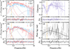 |
Fig. A.1. Same as Fig. 2 but using HXMT data. The selected energy bands are 1–3 keV for the reference band and 5–10 keV for the subject band. |
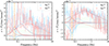 |
Fig. A.2. Linear-scale cross spectra from Fig. 2 (left) and Fig. 3 (right). Solid and dashed curves denote the QPO and individual non-QPO components, respectively. In both panels, data with absolute values ≤5 × 10⁻⁴ (light-blue region) are magnified by a factor of 3. |
We also present the CS of Figs. 2 and 3 on a linear y-axis, where the contributions of the Lorentzian components to the CS, or the data themselves, can be negative. Such details were not displayed in the main text (Sect. 4.1).
Appendix B: Energy dependence of lag and coherence across the full frequency range
Figure B.1 shows the energy evolution of the coherence and phase lags for four subject bands (NICER 5–8 keV, HXMT/LE 5–10 keV, HXMT/ME 27–35 keV, and HXMT/HE 50–65 keV; Day 7 at the outburst peak). In the softest band, the coherence remains near unity and exhibits only a shallow, symmetric dip at the QPO frequency. The corresponding phase lags display a mild, symmetric bump. Towards higher energies the dip broadens and deepens — approaching zero near the QPO frequency in the HXMT/HE band — while the phase lags evolve into a sharp, asymmetric shape, crossing from ≲ − 1 rad at low frequencies to positive values at the centroid frequency. Loss of coherence in XRBs can result from non-linear spectral responses (e.g. ionisation-dependent absorption and emission, thermal reverberation), spectral pivoting, and variability from spatially distinct or causally disconnected emission zones (e.g. Nowak et al. 1999; Ingram & Done 2009; Uttley et al. 2014; Grinberg et al. 2014; De Marco et al. 2020; Mastroserio et al. 2021).
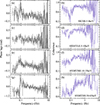 |
Fig. B.1. Frequency-resolved phase lags (left) and coherence (right) of 1A 0535+262 on Day 7. Reference bands are 0.2–2 keV (NICER) and 1–3 keV (HXMT/LE). Subject bands (top to bottom) are NICER 5–8 keV, HXMT/LE:5–10 keV, HXMT/ME:27–35 keV, and HXMT/HE:50–65 keV. A transition from symmetric, modest bumps to sharp ‘cliff’ structures is evident as energy increases, indicating the emergence of more pronounced QPO signatures in higher-energy bands. |
We attribute the observed behaviour to interference between multiple variability components present in the PS. As shown in the left panel of Fig. B.2, the broadband components display different energy-dependent phase lags. At low energies (red), these components exhibit similar phase lags and high coherence. At higher energies (brown and green), however, their phase offsets begin to diverge, which reduces coherence around the QPO and gives rise to the sharp, cliff-like lag features seen at higher energies.
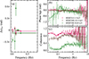 |
Fig. B.2. Panel (a): Phase lag of the fitted Lorentzian components (Δϕlor) versus frequency for three subject bands (HXMT/LE 3–5 keV, HXMT/ME 10–35 keV, and HXMT/HE 50–65 keV; colours as labelled), measured relative to the HXMT/LE 1–3 keV reference band. Panels (b) and (c): Frequency-resolved phase lags and coherence, respectively, for the same bands. Solid curves show the best-fit models. |
The above discussion can be formulated in the framework of Vaughan & Nowak (1997), in which the observed light curves are modelled as the sum of multiple variability components contributing simultaneously to both energy bands, x(t) = q1(t)+r1(t) and y(t) = q2(t)+r2(t), where q1(t) and q2(t) represent the contributions of the first component in the reference and subject bands, and r1(t) and r2(t) are those of the second component in the same bands. Let Q1 and Q2 denote the Fourier amplitudes of the first component in the two bands, and R1, R2 those of the second component. The phase lags of the two components between the bands are δθq and δθr, respectively.
The intrinsic coherence is given by
 (B.1)
(B.1)
When the two components are nearly out of phase (i.e. δθr − δθq ≈ π rad), the last term in the numerator becomes negative, leading to significant suppression of γxy2. In our case, this condition — corresponding to the largest phase lag difference — is most strongly satisfied by the high-energy bands, consistent with the observed spectral features. These findings suggest that, in 1A 0535+262, the energy dependence of both the lag and coherence spectra is primarily governed by interference between multiple quasi-periodic and broadband components, with phase coupling strongly modulated by energy.
Appendix C: Regrouped observations
NICER and HXMT observation log and QPO parameters for 1A 0535+262.
All Tables
All Figures
|
Fig. 1. Long-term X-ray light curves of the 2020 outburst of 1A 0535+262. Top panel: NICER count rate in the 0.2–12 keV band. Each observation is represented by a purple square. Bottom panel: HXMT light curves from the Core Science Program (P0314316). The LE (1–10 keV), ME (10–35 keV), and HE (27–250 keV) count rates are represented by the black (bottom), green (middle), and red (top) triangles, respectively. Additional observations from proposal P0304099 (PI: P. Reig) are marked with circles. Each data point represents a single observational epoch. The shaded grey region denotes the interval during which the millihertz QPO was most significantly detected at energies above 27 keV (Ma et al. 2022) and selected for cross-spectral analysis. |
| In the text | |
|
Fig. 2. Joint fit to the NICER data of 1A 0535+262 from Day 1. (a) PS of the reference (0.2–2 keV; blue) and subject (8–12 keV; red) bands. (b) 45°-rotated CS: Rerot (blue) and Imrot (red; QPO Rerot sign-flipped; see Fig. A.2a). In (a) and (b), solid and dashed curves show the total five-Lorentzian model and individual components. (c) Coherence and (d) phase lags, with models including (solid) and excluding (dashed) the QPO. Dash-dotted yellow line marks the QPO centroid frequency, which coincides with a coherence dip and phase-lag rise. Data above ∼1 Hz are logarithmically re-binned with a factor of exp(1/10). Bottom sub-panels: Residuals, Δχ = (data − model)/error. |
| In the text | |
|
Fig. 3. Same layout as Fig. 2 but for HXMT data. The reference and subject bands are 1–3 and 50–65 keV, respectively. Negative Lorentzian contributions to Rerot or Imrot are plotted with reversed signs; see Fig. A.2b. |
| In the text | |
|
Fig. 4. Energy dependence of the millihertz QPO properties in 1A 0535+262 for three epochs (MJD 59169, 59172, and 59181; corresponding to Days 3, 6, and 15). Top panel: Fractional rms amplitude as a function of energy. Bottom panel: Energy-resolved phase lag, ΔϕQPO, measured with respect to the reference band. Triangles and squares denote HXMT and NICER measurements, respectively. Colours indicate the outburst phase: red (rise), blue (peak), and green (decay). In each energy band, the QPO was modelled with a single Lorentzian component. |
| In the text | |
|
Fig. 5. Time evolution of millihertz QPO parameters in 1A 0535+262 during the 2020 outburst. Left three panels: Centroid frequency, HWHM, and rms amplitude of the QPOs as functions of MJD. Right panel: QPO phase lag (ΔϕQPO) for the energy bands listed in the legend, measured relative to 0.2–2 keV for NICER and 1–3 keV for HXMT. NICER data are shown in grey and HXMT data in violet. The QPO signal in each energy band was fitted with a single Lorentzian component. |
| In the text | |
|
Fig. 6. Single- and double-QPO fits to the HXMT/HE 50–65 keV subject band on Day 5 (MJD 59171; panels a–d) and Day 8 (MJD 59174; panels e–h), shown for the PS νPν and the corresponding phase-lag spectrum relative to the HXMT/LE 1–3 keV reference band. Panels (a), (c), (e), and (g): Single-QPO model (five Lorentzians; solid red curves). Panels (b), (d), (f), and (h): Double-QPO model (six Lorentzians; solid green curves). Dashed curves denote individual Lorentzian components; in the double-QPO model, the LF and HF QPO peaks are highlighted with dashed red and blue curves, respectively, consistent with Fig. 7. Residuals (Δχ) are shown beneath each spectrum. |
| In the text | |
|
Fig. 7. Energy dependence of the double-peak QPO properties in 1A 0535+262 on MJD 59171 and 59174. Top panels: rms amplitude as a function of energy. Bottom panels: Phase lags (ΔϕQPO). The filled blue and open red triangles represent the HF and LF QPOs, respectively. The differences in both rms amplitude (∼4.5% on Day 5 and ∼6.6% on Day 8) and phase lag (∼0.9π rad) remain approximately constant across the 27–120 keV energy range. |
| In the text | |
|
Fig. 8. Luminosity–phase–lag relation of the millihertz QPO in 1A 0535+262. ΔϕQPO in different energy bands (colours as in Fig. 5) versus bolometric luminosity. The light blue shaded region indicates the transition range, Lrev ∼ 1.11 − 1.16 × 1038. A transient soft lag appears only for L ≳ Lrev. All QPOs were fitted with a single-component model. |
| In the text | |
|
Fig. A.1. Same as Fig. 2 but using HXMT data. The selected energy bands are 1–3 keV for the reference band and 5–10 keV for the subject band. |
| In the text | |
|
Fig. A.2. Linear-scale cross spectra from Fig. 2 (left) and Fig. 3 (right). Solid and dashed curves denote the QPO and individual non-QPO components, respectively. In both panels, data with absolute values ≤5 × 10⁻⁴ (light-blue region) are magnified by a factor of 3. |
| In the text | |
|
Fig. B.1. Frequency-resolved phase lags (left) and coherence (right) of 1A 0535+262 on Day 7. Reference bands are 0.2–2 keV (NICER) and 1–3 keV (HXMT/LE). Subject bands (top to bottom) are NICER 5–8 keV, HXMT/LE:5–10 keV, HXMT/ME:27–35 keV, and HXMT/HE:50–65 keV. A transition from symmetric, modest bumps to sharp ‘cliff’ structures is evident as energy increases, indicating the emergence of more pronounced QPO signatures in higher-energy bands. |
| In the text | |
|
Fig. B.2. Panel (a): Phase lag of the fitted Lorentzian components (Δϕlor) versus frequency for three subject bands (HXMT/LE 3–5 keV, HXMT/ME 10–35 keV, and HXMT/HE 50–65 keV; colours as labelled), measured relative to the HXMT/LE 1–3 keV reference band. Panels (b) and (c): Frequency-resolved phase lags and coherence, respectively, for the same bands. Solid curves show the best-fit models. |
| In the text | |
Current usage metrics show cumulative count of Article Views (full-text article views including HTML views, PDF and ePub downloads, according to the available data) and Abstracts Views on Vision4Press platform.
Data correspond to usage on the plateform after 2015. The current usage metrics is available 48-96 hours after online publication and is updated daily on week days.
Initial download of the metrics may take a while.