| Issue |
A&A
Volume 696, April 2025
|
|
|---|---|---|
| Article Number | A128 | |
| Number of page(s) | 18 | |
| Section | Astrophysical processes | |
| DOI | https://doi.org/10.1051/0004-6361/202453092 | |
| Published online | 09 April 2025 | |
The nature of an imaginary quasi-periodic oscillation in the soft-to-hard transition of MAXI J1820+070
1
Instituto Argentino de Radioastronomía (CCT La Plata, CONICET; CICPBA; UNLP), C.C.5, 1894 Villa Elisa, Argentina
2
Facultad de Ciencias Astronómicas y Geofísicas, Universidad Nacional de La Plata, 1900 La Plata, Argentina
3
Kapteyn Astronomical Institute, University of Groningen, PO BOX 800 NL-9700 AV Groningen, The Netherlands
4
Key Laboratory of Particle Astrophysics, Institute of High Energy Physics, Chinese Academy of Sciences, Beijing, 100049
China
5
Dongguan Neutron Science Center, 1 Zhongziyuan Road, Dongguan, 523808
China
6
Center for Astrophysics | Harvard & Smithsonian, 60 Garden Street, Cambridge, MA, 02138
USA
7
Dr. Karl Remeis-Observatory and Erlangen Centre for Astroparticle Physics, Friedrich-Alexander-Universität Erlangen-Nürnberg, Sternwartstr. 7, 96049 Bamberg, Germany
⋆ Corresponding author.
Received:
20
November
2024
Accepted:
14
February
2025
A recent study shows that if the power spectra (PS) of accreting compact objects consist of a combination of Lorentzian functions that are coherent in different energy bands but incoherent with each other, the same is true for the real and imaginary parts of the cross spectrum (CS). Using this idea, we discovered imaginary quasi-periodic oscillations (QPOs) in NICER observations of the black hole candidate MAXI J1820+070. The imaginary QPOs appear as narrow features with a small real and large imaginary part in the CS but are not significantly detected in the PS when they overlap in frequency with other variability components. The coherence function drops and the phase lags increase abruptly at the frequency of the imaginary QPO. We show that the multi-Lorentzian model that fits the PS and CS of the source in two energy bands correctly reproduces the lags and the coherence, and that the narrow drop in the coherence is caused by the interaction of the imaginary QPO with other variability components. The imaginary QPO appears only in the decay of the outburst, during the transition from the high-soft to the low-hard state of MAXI J1820+070, and its frequency decreases from ∼5 Hz to ∼1 Hz as the source spectrum hardens. We also analysed the earlier observations of the transition, where no narrow features were seen, and we identified a QPO in the PS that appears to evolve into the imaginary QPO as the source hardens. As for the type-B and C QPOs in this source, the rms spectrum of the imaginary QPO increases with energy. The lags of the imaginary QPO are similar to those of the type-B and C QPOs above 2 keV but differ from the lags of those other QPOs below that energy. While the properties of this imaginary QPO resemble those of type-C QPOs, we cannot rule out that it is a new type of QPO.
Key words: accretion / accretion disks / stars: black holes / X-rays: binaries / X-rays: individuals: MAXI J1820+070
© The Authors 2025
 Open Access article, published by EDP Sciences, under the terms of the Creative Commons Attribution License (https://creativecommons.org/licenses/by/4.0), which permits unrestricted use, distribution, and reproduction in any medium, provided the original work is properly cited.
This article is published in open access under the Subscribe to Open model. Subscribe to A&A to support open access publication.
1. Introduction
Black hole X-ray binaries (BHXBs), consisting of a black hole and a secondary star, exhibit X-ray outbursts driven by mass accretion onto the black hole (Bahramian & Degenaar 2023). As they transition through different X-ray spectral states (Méndez & van der Klis 1997; Belloni et al. 2005), BHXBs describe a ‘q’ shape in the hardness intensity diagram (HID; Homan et al. 2001). In a typical outburst, a transient BHXB starts in the low hard state (LHS), with a relatively low X-ray intensity and a hard energy spectrum (Méndez & van der Klis 1997; Belloni et al. 2005). During this state, the source follows an almost vertical path in the diagram as the intensity increases and the hardness ratio decreases slightly (Belloni et al. 2011). Eventually, the source spectrum softens at an essentially constant intensity, and the BHXB transitions to the hard and soft intermediate states (HIMS and SIMS, respectively; Homan & Belloni 2005). As the outburst continues, the source then reaches the high soft state (HSS) where the energy spectrum is soft and the intensity decreases while its hardness remains more or less constant (Méndez & van der Klis 1997; Belloni et al. 2005, 2011). Finally, at the decay of the outburst, the BHXB returns to the LHS, completing the q shape in the diagram (Belloni 2010).
Black hole X-ray binaries exhibit fast X-ray variability throughout outbursts, offering crucial insights into the dynamics of the accretion processes around the compact object (van der Klis 1994, 2006; Belloni et al. 2011). The analysis of this variability is key to understanding the mechanisms of accretion and ejection involved in these systems (van der Klis 1994; Fender et al. 2004; Ingram et al. 2009; Kara et al. 2019; Mastroserio et al. 2019, see Motta 2016 for a review). The power spectrum (PS) of these sources presents relatively narrow peaks called quasi-periodic oscillations (QPOs), which are among the most notable features of the variability (van der Klis 1989; Nowak 2000; Belloni et al. 2002, see Ingram & Motta 2019 for a review). Low-frequency QPOs (LFQPOs) in BHXBs have frequencies ranging from a few milliHertz to ∼30 Hz (Belloni et al. 2002; Casella et al. 2004; Remillard & McClintock 2006; Motta et al. 2012). LFQPOs are classified into three types (Wijnands et al. 1999; Remillard et al. 2002; Casella et al. 2004, 2005, for reviews, see Motta 2016; Belloni & Motta 2016), A, B and C, based on their centroid frequency, ν0, quality factor Q = (ν0/FWHM), where FWHM is the full width half maximum of the QPO, fractional root mean square (rms) amplitude, phase lags, and the strength and shape of the broadband noise in the PS (Casella et al. 2004). Among these, type-C QPOs are the most common in BHXBs (Motta et al. 2012). These QPOs are strong, with rms amplitudes that can reach up to 20%, and they are generally observed in the LHS and the HIMS (Casella et al. 2004; Motta et al. 2011). Type-C QPOs have centroid frequencies in the range of 0.1 − 15 Hz and high quality factors, normally above ten (Casella et al. 2004; Belloni et al. 2005; Motta et al. 2011). On the other hand, type-B QPOs are weaker, with rms amplitudes lower than 5%, and centroid frequencies around 6 Hz (Casella et al. 2004, 2005). These QPOs appear only in the SIMS, distinguishing this state from the HIMS (Motta et al. 2011). Type-B QPOs usually have quality factors above six and are accompanied by weak red noise (Casella et al. 2004, 2005). Type-A QPOs are the weakest LFQPOs and they usually appear just after the source transitions into the HSS with frequencies around 6 − 8 Hz (Belloni & Stella 2014).
The Fourier CS between simultaneous light curves in two energy bands is employed to derive the frequency-dependent phase lags between those two energy bands (van der Klis et al. 1987; Vaughan et al. 1997; Nowak et al. 1999a; Uttley et al. 2014), which give the phase angle of the cross vector in the complex Fourier plane (Vaughan & Nowak 1997). Furthermore, the CS and the PS of the two time series can be used to obtain the coherence function. The coherence function is a measure of the degree of linear correlation between the two simultaneous time series as a function of the Fourier frequency (Bendat & Piersol 2011; Vaughan & Nowak 1997), and it allows us to identify a particular frequency or range of frequencies that are strongly correlated across energy bands (Nowak et al. 1999a). The coherence function is a valuable tool for studying processes characterised by features such as QPOs or abrupt changes in slope in the PS (Nowak et al. 1999a). Vaughan & Nowak (1997) showed that if there are multiple signal components contributing to the data in two energy bands, the coherence function may fall below unity, even if each individual component generates perfectly coherent variability.
Méndez et al. (2024) present a novel method to measure the lags of variability components in low-mass X-ray binaries (LMXBs). Employing a multi-Lorentzian model –a linear combination of Lorentzian functions– the authors fit the PS and the real and imaginary parts of the CS simultaneously. Méndez et al. (2024) assume that both the PS and the CS comprise several components that are coherent in different energy bands but incoherent with each other. In that case, the real and imaginary parts of the CS are linear combinations of the same Lorentzians but each of them is respectively multiplied by the cosine or sine of a function that represents the phase lag between the corresponding Lorentzian in each signal and it is, in principle, frequency-dependent. Once they found the best fit for the PS and the CS, they could derive the model that predicts the lags and coherence function.
The technique introduced by Méndez et al. (2024) allowed them to unveil variability components that were not significantly detected in the PS but were significant in the CS. Using this method, the authors found a narrow QPO in an observation of the BHXB MAXI J1820+070 that was very significant in the imaginary part of the CS but was not detected in the PS. They refer to this QPO as ‘imaginary QPO’ since it has a large imaginary but a small real part in the CS. This signal overlaps in frequency with other signals with large real parts, which leads to a narrow drop in the coherence function at the imaginary QPO frequency (first observed by König et al. 2024, see also Ji et al. 2003).
MAXI J1820+070 is an X-ray transient discovered with the Monitor of All-Sky X-ray Image (MAXI; Matsuoka et al. 2009) in 2018 (Kawamuro et al. 2018), when the source underwent an outburst. MAXI J1820+070 was closely monitored by the Neutron Star Interior Composition Explorer (NICER; Gendreau et al. 2016), almost daily from March 6 to November 21; within these dates, the source exhibited significant spectral changes, describing an overall q shape in the HID. During the transition from the LHS to the HSS, a type-C QPO present in the X-ray power of MAXI J1820+070 switched to a type-B QPO (Homan et al. 2020). Ma et al. (2023) studied the observation that covered the transition of the QPO types (obsID 1200120297) and obtained the rms and phase lag spectra of both types of QPOs. Ma et al. (2023) found that above 1.5 − 2.0 keV, the rms and lag spectra of the two types of QPOs are similar, but they are significantly different at lower energies: below 1.5 − 2.0 keV, the type-B QPOs show a smaller rms amplitude and softer phase lags than the type-C QPOs.
The purpose of this work is to expand the analysis carried out by Méndez et al. (2024), searching for other observations of MAXI J1820+070 that exhibit the drop in the coherence to study the properties of the imaginary QPO. In Sect. 2 we show why a variability component with a large imaginary part in the CS, when overlapping in frequency with a component with a large real part, can be undetectable in the PS but significantly detected in the CS. In Sect. 3 we describe the observations and data reduction of MAXI J1820+070. In Sect. 4 we present the results obtained from the analysis of the MAXI J1820+070 data that exhibit a drop in the coherence. We then fit those observations and we study the properties of the imaginary QPO. Finally, in Sect. 5 we discuss our findings.
2. Hidden variability
The novel method presented by Méndez et al. (2024) allows us to detect variability components that are not detected in the PS but are significant in the CS. As demonstrated in the following paragraphs, this happens when a signal that has a large imaginary part but a small real part in the CS overlaps in frequency with other signals that have a large real part.
Consider two correlated light curves of an LMXB measured in two energy bands, denoted as x(t) and y(t), with corresponding complex Fourier transforms X(ν) and Y(ν). Following the notation in Méndez et al. (2024), we define the PS of both series as Gxx(ν) and Gyy(ν), the CS as Gxy(ν) = ⟨|X(ν)||Y(ν)|eiΔϕxy(ν)⟩, where Δϕxy(ν) is the phase lag between the two series at frequency ν, and the angle brackets indicate averaging over an ensemble of measurements of X(ν) and Y(ν) (for details, see Bendat & Piersol 2011). We define the intrinsic coherence function as γxy2(ν) = |Gxy; i(ν)|2/Gxx(ν)Gyy(ν). We subsequently consider two variability components overlapping in frequency, one with a phase lag of π/2, such that its real part in the CS, Re1(ν), is zero, and the other one with a phase lag of 0, such that its imaginary part, Im2(ν), is zero. We describe each variability component with a Lorentzian function, coherent in both energy bands but incoherent with each other. We assume that the variability components are additive (Nowak 2000; Belloni et al. 2002; Méndez et al. 2024), but there are other possibilities (see for instance Ji et al. 2003; Uttley et al. 2005; Ingram & van der Klis 2013; Zhou et al. 2022). We can write the following:
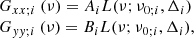
where i = 1, 2 refers to the ith variability component, Ai, Bi ∈ ℝ are the integrated power, from zero to infinity, of the Lorentzian components in each of the two energy bands and ν0; i and Δi are, respectively, the centroid frequency and the FWHM of the Lorentzians. These two Lorentzian parameters, ν0; i and Δi, are the same in both energy bands, assuming that each input process is perfectly coherent with the corresponding output process.
Under the assumption that for each Lorentzian function γxy; i2(ν) = 1, |Gxy; i(ν)|2 = AiBiL2(ν; ν0; i, Δi), and from the choice that the first component has a zero real part (Δϕxy; 1(ν) = π/2) and the second component a zero imaginary part (Δϕxy; 2(ν) = 0):
![$$ \begin{aligned} \begin{array}{ll}&\mathrm{Im}[G_{xy;1}]= \sqrt{A_1 B_1} \\&\mathrm{Re}[G_{xy;2}]= \sqrt{A_2 B_2}, \end{array} \end{aligned} $$](/articles/aa/full_html/2025/04/aa53092-24/aa53092-24-eq2.gif)
where Gxy; i = ∫0∞Gxy; i(ν)dν.
Let us posit two additional assumptions regarding the considered variability components:
-
(i)
Component 2 is stronger than Component 1: Re[Gxy; 2] ≫ Im[Gxy; 1] and therefore, A2B2 ≫ A1B1;
-
(ii)
The rms spectrum of both components is similar, such that B2/A2 = B1/A1 = :k.
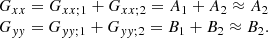
Combining these two hypotheses, we have that A2 ≫ A1 and B2 ≫ B1, and we can approximate the total PS as:
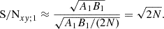
The error for the imaginary part of the CS (Bendat & Piersol 2011; Ingram 2019), is:
![$$ \begin{aligned} \mathrm{dIm} [G_{xy}] = \sqrt{\frac{G_{xx} G_{yy}-\mathrm{Re}^2[G_{xy;2}] + \mathrm{Im}^2[G_{xy;1}]}{2N}} \approx \sqrt{\frac{A_1B_1}{2N}}, \end{aligned} $$](/articles/aa/full_html/2025/04/aa53092-24/aa53092-24-eq4.gif)
where N is the product of the number of segments used to compute the CS and the number of frequency bins in the range in which we measure the CS. Hence, the signal-to-noise ratio (S/N) of the Component 1 in the CS is:
As a consequence, given a sufficient number of segments, Component 1 will attain significance in the imaginary part of the CS.
For the PS in each energy band, using (ii), we can write Eq. (2) as ![$ \mathrm{Im} [G_{xy;1}]= \sqrt{k}A_1 $](/articles/aa/full_html/2025/04/aa53092-24/aa53092-24-eq6.gif) and
and ![$ \mathrm{Re} [G_{xy;2}]= \sqrt{k}A_2 $](/articles/aa/full_html/2025/04/aa53092-24/aa53092-24-eq7.gif) , and it is easy to show that:
, and it is easy to show that:
![$$ \begin{aligned} \mathrm{d}G_{xx} \approx \frac{\mathrm{Re} [G_{xy;2}]}{\sqrt{kN}}= \frac{A_2}{\sqrt{N}};~~~~~~~~ \mathrm{d}G_{yy} \approx \frac{B_2}{\sqrt{N}}. \end{aligned} $$](/articles/aa/full_html/2025/04/aa53092-24/aa53092-24-eq8.gif)
Hence, the S/N of the Component 1 in each PS is:
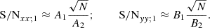
Subsequently, since A2 ≫ A1 and B2 ≫ B1, the S/N of the Component 1 increases with N much more slowly in the PS than in the CS.
We have demonstrated that a QPO characterised by a large imaginary part and a small real part in the CS can be hidden in the PS, while being significant in the CS. We emphasise Méndez et al. (2024) conclusion that searching for QPOs exclusively in the PS may lead to overlooking significant variability components. In the next sections, we use these considerations to study the variability of MAXI J1820+070.
As shown in Bendat & Piersol (2011), the error of the coherence function is 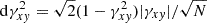 . Therefore, when the coherence function is close to unity, its estimates can be more accurate than those of the PS or CS. Consequently, variability components hidden in both PS and CS could have a large S/N in the coherence function. Given its greater sensitivity, the coherence function may allow us to uncover new signals that could be missed by looking only at the PS and CS.
3. Observations and data analysis
We used the tool nicerl2 to process the NICER data of MAXI J1820+070 and produce the clean event files. We computed the PS in two energy bands, 0.3 − 2.0 keV and 2.0 − 12.0 keV, and the CS between the same bands using GHATS1. We calculated the Fast Fourier transform (FFT) in each band, setting the length of the segment to 65.536 s and the time resolution to 0.4 ms, which results in a lowest frequency of 0.015 Hz and a Nyquist frequency of 1000 Hz. GHATS generates the Leahy normalised PS and CS for each segment, which are then averaged to produce the PS and CS of the observation. To correct for the Poisson level in the PS, we subtracted the average power in the frequency range 400 − 800 Hz. To increase the S/N at intermediate and high frequencies, we performed a logarithmic rebinning, increasing the size of each bin by a factor 101/100 compared to the previous bin. We finally normalised the PS and CS to fractional rms units, ignoring the background since its contribution to the total count rate is negligible. GHATS also computes the phase-lag and the coherence-function frequency spectra. We took the energy band 0.3 − 2.0 keV as the reference band when computing the CS and phase-lag frequency spectrum.
We note that the phase lags of MAXI J1820+070 during these observations are close to zero over a broad range of frequencies, meaning that the imaginary part of the CS is much smaller than the real part at all Fourier frequencies. We therefore rotated all cross vectors by 45 degrees to have approximately equal real and imaginary parts. As explained in Méndez et al. (2024), this rotation would make an eventual fit of the CS more stable without having any impact on the best-fitting parameters.
We processed the data of 131 NICER observations, from obsID 1200120101 to 1200120293, that correspond to MJD 58190 − 58443. We computed the light curve of MAXI J1820+070 for each observation in the 0.5 − 12.0 keV band. We used nicer3-lc to normalise the light curves by the number of active focal plane modules (FPMs) that, in some cases, had to be lowered to avoid data dropouts caused by saturation when the source was too bright. Defining the hardness ratio as the ratio of the count rates in the 2.0 − 12.0 keV to that in the 0.5 − 2.0 keV, we produced the hardness intensity diagram (HID).
We explored the phase lags and coherence function for all the observations, aiming to identify sharp features that could result from the overlapping in frequency of two or more variability components. For the observations in which this was the case, we repeated the procedure to generate the PS and CS but using two hard energy bands, 2.0 − 5.0 keV and 5.0 − 12.0 keV, and we examined if those features remained visible.
We used XSPEC v.12.13.0c to fit simultaneously the PS in the 0.3 − 2.0 keV and 2.0 − 12.0 keV bands and the real and imaginary parts of the CS in the same energy bands, considering the 0.01 − 50 Hz frequency range. We began by fitting simultaneously the PS in both bands with a single Lorentzian function and we added Lorentzians until the reduced χ2 was about unity and there were no systematic trends in the residuals. The multi-Lorentzian model obtained from this phenomenological approach serves as a starting point to fit simultaneously both PS and the real and imaginary parts of the CS assuming constant phase lags with Fourier frequency for each component (Méndez et al. 2024). We linked the centroid frequencies and FWHM of each Lorentzian in the two PS and in the CS but we left the normalisations of the PS free to vary independently. For each Lorentzian, its normalisation in the CS was tied to the square root of the product between the two PS normalisations. If necessary, we added more Lorentzians until we obtained a good fit, considering also the residuals of the CS.
From the best-fitting model, we derived the model for the phase lags and the coherence function. While we plotted the phase-lag spectrum and the coherence function with the derived model, it is important to note that we did not fit those data; rather those models are a prediction of the multi-Lorentzian model used to fit PS and CS.
To explore the energy dependence of the rms amplitude and phase lags of a QPO, we extracted the PS in six energy bands: 0.3 − 1.0, 1.0 − 1.5, 1.5 − 2.5, 2.5 − 4.0, 4.0 − 5.0, 5.0 − 12.0 keV. We also generated the CS of each band with respect to the total band 0.3 − 12 keV, which was therefore the reference band for the lags. As usual, we refer to hard lags when the high-energy photons lag the low-energy ones, and to soft lags when the opposite occurs. To correct for the partial correlation of the photons that are simultaneously in the narrow and the total energy bands, we subtracted the average of the real part of the CS calculated in a frequency range where the source does not contribute (Belloni et al. 2024; Méndez et al. 2024). Using the best-fitting model for each observation with the centroid frequencies and FWHMs of every Lorentzian fixed, we fitted simultaneously the PS in a small band of energy, the PS in the total band and the real and imaginary parts of the CS. We then constructed the amplitude and phase-lag spectra using the parameter values of the Lorentzian corresponding to the QPO in each small energy band: the rms amplitude at that energy band is the square root of the Lorentzian normalisation, and the phase lag is the argument of the cosine and the sine functions that multiply the Lorentzian in, respectively, the real and imaginary parts of the CS.
4. Results
The left panel of Fig. 1 shows the evolution of the NICER count rate of the source in the 0.5 − 12 keV band during the outburst. Each data point represents one obsID from 1200120101 to 1200120293, which corresponds to MJDs between 58189 and 58424. Throughout this period, the source traced an overall q shape in the HID, as shown in the right panel of Fig. 1. At the beginning of the outburst, MAXI J1820+070 is in the LHS and its count rate increases rapidly from ∼16 cts s−1 FPM−1 to ∼360 cts s−1 FPM−1 as the source transitions to the intermediate state. At that point, the count rate stays more or less constant, except for a small valley between MJD 58262 − 58305 that reaches a minimum of ∼106 cts s−1 FPM−1. The source then enters the HSS, where the count rate decreases slowly from ∼1200 cts s−1 FPM−1 to ∼550 cts s−1 FPM−1. Around MJD 58380, MAXI J1820+070 leaves the HSS and the count rate drops rapidly as the source returns to the LHS, reaching ∼1.2 cts s−1 FPM−1 by the last observation considered. Days after approaching quiescence (Russell et al. 2019), MAXI J1820+070 underwent three reflares (Ulowetz et al. 2019; Hambsch et al. 2019; Adachi et al. 2020), but we do not analyse them in this study.
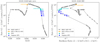 |
Fig. 1. NICER X-ray light curve (left panel) and hardness-intensity diagram (right panel) of MAXI J1820+070 during its 2018 outburst. The intensity in both panels is the count rate per detector in the 0.5 − 12 keV band, while the hardness ratio in the right panel is the ratio of the count rates in the 2 − 12 keV to that in 0.5 − 12 keV. Each point corresponds to one obsID within 1200120101 − 1200120293. Light blue diamonds (obsIDs 1200120263 − 1200120265) and blue dots (obsIDs 1200120266 − 1200120270) depict the observations considered in this paper, in particular, the second ones correspond to those presenting narrow features in the phase lags and the coherence function. The orange star represents the observation 1200120197 studied by Ma et al. (2023), which covered the transition of type-C to a type-B QPO. |
We examine the phase lags and coherence function of all 131 observations searching for significant features, such as sharp drops or abrupt changes, which may indicate overlapping variability components and potentially unveil a hidden component in the PS. We identify some observations in the HIMS at the upper part of the q where a shallow drop in the coherence coincides with a QPO in the PS. Furthermore, we note that, during five observations in the lower branch of the q, where the source is transitioning back to the LHS, the coherence exhibits a more pronounced and significant drop at a frequency at which, in principle, no QPO is visible in the PS. At the same frequency of this coherence feature, we observe an abrupt jump in the phase lags that resembles a ‘cliff’. These observations provide an excellent opportunity to apply the derived model presented in Méndez et al. (2024) and assess its predictive capability. Therefore, aiming to identify a variability component hidden in the PS that can explain these significant features, we focus on these five observations, which are highlighted in blue in Fig. 1 and correspond to ObsIDs from 1200120266 to 1200120270.
To encompass the complete HSS-to-LHS transition, we extend the analysis to include the obsIDs 1200120263, 1200120264 and 1200120265, depicted with light blue diamonds in Fig. 1. Before observation 1200120263, MAXI J1820+070 was in the HSS, where the rms amplitude of the variability is very low. After observation 1200120270, there was a nine-day gap in the data. In the following observation, the source was already in the LHS with a count rate almost an order of magnitude lower, and therefore much weaker.
In Fig. 2 we show the phase lags (left panels) and the coherence function (right panels) for each observation of the HSS-to-LHS transition. In the first three observations, no significant features are visible. For the following observations, in the left panels, we see that the phase lags increase more or less steeply at the frequency marked by the dashed red line, and then decrease more or less smoothly as the frequency increases, resembling a cliff; the cliff moves to lower frequencies as the spectrum of MAXI J1820+070 hardens. Concomitantly, in the right panels, we see a sharp drop in the coherence function that moves to lower frequencies as the source approaches the LHS.
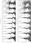 |
Fig. 2. Phase lags (left panels) and intrinsic coherence function (right panels) for NICER observations from 1200120263 to 120012070 of MAXI J1820+070 for the 0.3–2 keV and 2–12 keV energy bands. With a dashed red line, we depict the frequency of the imaginary QPO in each observation derived from the multi-Lorentzian fitting approach (see Sect. 4.1 for details). |
In particular, during observations 1200120264 and 1200120266, the source exhibited a significant change in the count rate. We examine the dynamical power spectra and observe notable differences in the power behaviour between the two periods. Therefore, for the subsequent analysis, we divide those observations into two segments, named p1 and p2. For observation 1200120264, the segments correspond to orbits 1 and 2-4, and for observation 1200120266, they correspond to orbits 1 and 2-5. For convenience, we hereafter refer to each of these segments as an ‘observation’.
4.1. Imaginary QPO
In this section, we present the results of fitting the NICER observations during the HSS-to-LHS transition of MAXI J1820+070. As explained in Sect. 3, for each observation we start by simultaneously fitting a multi-Lorentzian model to the PS in two energy bands, 0.3 − 2.0 keV and 2.0 − 12.0 keV, considering almost 4 frequency decades, from 0.01 Hz to 50 Hz. We then use this model as a starting point to fit both PS and the real and imaginary parts of the CS following the method introduced by Méndez et al. (2024) assuming constant phase lags. In every case, we add the number of Lorentzian functions needed to obtain a reduced χ2 near 1 and residuals without trends. In this phenomenological approach, all of the Lorentzian components have a significance of at least 3 − σ in either the PS, the CS or both, which we measure from the error (the negative one if the errors are asymmetric) of the normalisation of the Lorentzian. In the first observation, we fit a model with four Lorentzians; for the following two observations, a model with three; for the next six observations, a model with five; and for the last one, a model of six Lorentzians provides a good fit. In Appendix A, we present the best-fitting models for each observation (see Fig. A.1), as well as the best-fitting parameters with their 1 − σ uncertainties (see Table A.1). We use the derived model explained in Méndez et al. (2024) to predict the behaviour of the phase lags and the coherence function.
We use observation 1200120268 as an example to show our findings. The best fit of these data with a five-Lorentzian model gives a χ2 ≈ 992 for 823 d.o.f. In the top panels of Fig. 3 we present the best fit to the two PS (left) and the real and imaginary parts of the CS (right), with their corresponding residuals. In the bottom panels of Fig. 3 we show the prediction of the derived model for the phase lags (left) and the coherence function (right). We note that the behaviour of both of them is well-reproduced by the model. Around 2.06 Hz, the coherence drops significantly, while the phase lags become abruptly harder. We plot a dashed vertical line at 2.06 Hz in every panel, corresponding to the centroid frequency of one of the QPOs in the model. We refer to this QPO as the imaginary QPO, since it has a large imaginary part and a small real part in the CS. While this imaginary QPO is not significant in either of the PS, it is needed in the CS and it is responsible for the narrow drop in the coherence function.
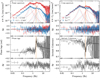 |
Fig. 3. Top left panel: PS of NICER observation 1200120268 of MAXI J1820+070 in two energy bands. The 0.3–2 keV data are shown in blue while the 2–12 keV one is in red, both with the best-fitting model (solid line) consisting of 5 Lorentzian functions (dotted lines). Top right panel: real and imaginary parts of the CS between the same two energy bands rotated by 45°. We plot Re cos(π/4)−Im sin(π/4) in blue and Re sin(π/4)+Im cos(π/4) in red, with the best-fitting model assuming constant phase lags. Bottom panels: Phase-lag spectrum (left) and intrinsic coherence function (right) with the derived model (solid line) obtained from the fit to the PS and CS. In all four panels, residuals with respect to the model, defined as Δχ = (data − model)/error, are also plotted. The dashed orange vertical line at 2.06 Hz in every panel corresponds to the centroid frequency of the imaginary QPO in the model. |
Previous studies have fitted the PS of MAXI J1820+070 with two or three broad components (e.g. Kawamura et al. 2023). This may appear to contradict the need to use up to five Lorentzians to fit the PS and the CS simultaneously. For instance, Veledina (2016) suggested that peaked noise observed in the PS of accreting BHXBs could be the result of the interference of two broad components, the disc Comptonisation and the synchrotron Comptonisation, both modulated by accretion rate fluctuations and separated by a time delay. To explore this idea, we attempt to fit the data with only two broad Lorentzians and assess whether such a model can explain the observed drop in the coherence. In doing this, we obtain structured residuals in the PS, CS, phase lags and coherence. In particular, the derived model for the coherence shows a broad and shallow drop, and at around 2 Hz the coherence shows narrow residuals at a ∼6σ level. In summary, a model with only two broad Lorentzians cannot fit the data. Specifically, this model does not reproduce the drop in the coherence at ∼2.1 Hz. The only way to recover the narrow and deep drop observed in the coherence data is to include the imaginary QPO.
Since König et al. (2024) remarked that the feature in the coherence function is only observed when an energy band below 2 keV is used, we also extract the PS in two hard energy bands, 2–5 keV and 5–12 keV, and the CS between these two energy bands for the observations considered in this work. We notice that the sharp features shown in Fig. 2, the narrow drop in the coherence and the cliff in the phase lags, are no longer detected in this case. Using the best-fitting model obtained for the energy bands 0.3–2 keV and 2–12 keV, we fit the data in these hard bands, fixing the centroid frequencies and FWHM of every Lorentzian, and we find that the imaginary QPO is not significant in any of the PS neither in the CS. The 95% confidence upper limit to the rms fractional amplitude of that Lorentzian in the PS corresponding to 5–12 keV is ∼4% and in the 2–5 keV and in the CS is ∼3%.
We use the same method described above to fit all the observations of the HSS-to-LHS transition of MAXI J1820+070. Moving backwards in time from observation 1200120268, we also identify the imaginary QPO that naturally explains the narrow features in the phase lags and coherence function. As in Méndez et al. (2024), we find that the peak of the cliff in the phase lags and the narrow drop in the coherence coincide with the centroid frequency of the imaginary QPO. These frequencies are marked with vertical dashed red lines in Fig. 2. As we move further back to earlier observations, the amplitude of the QPO decreases in the imaginary part of the CS, while it increases in the real part. Eventually, this variability component becomes significant in the power spectra and is no longer ‘imaginary’. We are able to track the evolution of not just the QPO but also other Lorentzian components by fitting a consistent multi-Lorentzian model to all observations of the HSS-to-LHS transition (see Fig. A.1). We note that these Lorentzian components jointly shift to higher frequencies for softer states of the source, preserving their relative order as they move in frequency. This consistency in the model allows us to identify the imaginary QPO as evolving from a ‘real’ QPO observed in the PS during the earlier stages of the HSS-to-LHS transition. In Fig. 4, we present the fit of the power spectra (left) and the real and imaginary parts of the CS (right) for observation 1200120265, with their corresponding residuals. In this case, the QPO, depicted by the vertical orange line, is needed to fit the PS. The derived models for the phase lags and coherence function (not shown) do not predict any narrow features, consistently with the observed behaviour in the earlier observations in Fig. 2. Henceforth, when describing the properties of the QPO across the earlier stages of HSS-to-LHS transition, where the imaginary part of the CS is smaller than the real one, we refer to it as the ‘real QPO’.
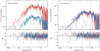 |
Fig. 4. Left panel: PS of NICER observation 1200120265 of MAXI J1820+070 in two energy bands. The 0.3 − 2 keV data are shown in blue while the 2 − 12 keV one is in red, both with the best-fitting model (solid line) consisting of 5 Lorentzian functions (dotted lines). Right panel: Real and imaginary parts of the CS between the same two energy bands rotated by 45°. We plot Re cos(π/4)−Im sin(π/4) in blue and Re sin(π/4)+Im cos(π/4) in red, with the best-fitting model assuming constant phase lags. In both panels, residuals with respect to the model, defined as Δχ = (data − model)/error, are also plotted. The dashed orange vertical line at 6.03 Hz in each panel corresponds to the centroid frequency of the QPO in the model. |
Moving forwards in time from observation 1200120268, we again detect the imaginary QPO only in the CS at the frequency of the narrow features in the phase lags and coherence function. In particular, the characterisation of the imaginary QPO in observation 1200120270 is less certain due to the reduced number of 65-seconds segments available for the analysis (see Table 1).
Best-fitting values of the QPO in MAXI J1820+070 for each observation with their corresponding 1-σ uncertainties.
4.2. Time-evolution of QPO properties
On the left panels of Fig. 5 we show the time-evolution of the rms amplitudes of the QPO in the hard (upper panel) and soft (bottom panel) energy bands, while on the right panel, we show the time-evolution of the phase lags of the QPO between those energy bands. The horizontal bars in the plot indicate the duration of each observation. In observation 1200120268, the rms amplitude of the imaginary QPO in the 2 − 12 keV energy band is ∼3.4%. As we move to earlier observations, the rms amplitude of the hard band increases up to ∼8.3% for observation 1200120265. Instead, for even earlier observations, the rms decreases to ∼2.7%. Regarding the 0.3 − 2 keV energy band, the rms amplitude for observation 1200120268 is ∼1.4%, and it remains more or less constant as we move back in time. For observation 1200120265, the rms amplitude rises to about ∼2.2% and decreases to ∼0.7% for earlier observations. On the right panel of Fig. 5, we observe that the phase lag for observation 1200120268 is ∼1.2 rad. We find smaller magnitudes of the phase lags corresponding to softer states of the source, consistent with the decreasing amplitude of the imaginary part and the increasing amplitude of the real part of the QPO. In observation 1200120264_p1, the QPO has a soft phase lag of ∼ − 0.4 rad that, being less than π/4 in magnitude, indicates that its real part is larger than its imaginary part. On the other hand, for observation 1200120269, the imaginary QPO has a large hard lag of ∼1.9 rad, its rms amplitude in the hard energy band is ∼2.5% and in the soft band, ∼1.1, respectively. For the following observation, the phase lag of the imaginary QPO decreases to ∼0.7 rad, while the rms amplitudes increase to ∼4% and ∼2.1%, respectively. We note that the centroid frequency of the QPO shows a general tendency to decrease as the source hardens, from 9.1 Hz to 1.1 Hz, as evidenced by the colour gradient in Fig. 5. A similar decreasing trend with frequency is observed for the other Lorentzians, which we can trace across the subsequent observations.
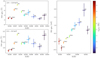 |
Fig. 5. Evolution of the rms amplitude of the QPO in the 2.0 − 12.0 keV band (top left) and in the 0.3 − 2.0 keV band (bottom left) as MAXI J1820+070 transitions out of the HSS. The right panel displays the evolution of the phase lags of the QPO for the 2.0 − 12.0 keV band with respect to the 0.3 − 2.0 keV band. The rms and phase lags are derived from the fitted Lorentzian in our model (see Sect. 3). In the three panels, the horizontal bars correspond to the time duration of each observation, while the vertical bars are the actual 1 − σ errors of each quantity. The colour gradient depicts the centroid frequency of the QPO. |
Motta et al. (2011) found a relation between the amplitudes of the broadband variability of the source GX339–4 and the QPO frequency for different QPO types. In their Fig. 4, Motta et al. (2011) plotted the broadband fractional rms of the PS integrated between 0.1 Hz and 64 Hz vs. the QPO centroid frequency, using RXTE data in the 2 − 20 keV energy range. They showed that different types of QPOs occupy different regions in the plot. In Fig. 6, we reproduce that plot for the QPOs in MAXI J1820+070 using NICER data in the 0.3 − 12 keV energy range and considering the 0.1 − 50 Hz frequency range. The blue dots and diamonds correspond to the imaginary and the real QPOs, respectively, in our considered observations. We also include the type B (yellow squares) and C (green triangles) QPOs identified by Ma et al. (2023) in different orbits of observation 1200120197 of MAXI J1820+070. The arrows indicate the time progression of these measurements. The difference in the direction in which the source moves is because in the orbits of 1200120197 (red), MAXI J1820+070 is softening while in our observations (blue) the source is hardening. We see that, as the source transitions towards the LHS, the QPO frequency decreases and the total variability increases from ∼11.7% to ∼27%. The rms amplitudes of the type C QPO span from ∼8% to ∼15% while those of the type B QPO are between ∼3% and ∼5%. For both type B and C QPOs we find smaller rms amplitudes than the values in GX 339−4 in Motta et al. (2011).
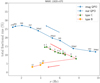 |
Fig. 6. Total fractional rms in the 0.3–12 keV band integrated from 0.1 to 50 Hz versus the centroid frequency of the QPO in MAXI J1820+070 (blue), with both quantities derived from our fitted model. Diamonds correspond to observations 1200120263-1200120265 while dots correspond to observations 1200120266_p1-1200120270. Green triangles and orange squares depict the type B and C QPOs identified in each orbit of observation 1200120197, which covered the HIMS-SIMS transition, studied by Ma et al. (2023). The solid and dashed lines connect the QPOs during the source hardening and softening respectively. Arrows indicate the direction of time progression in each sequence. |
In Table 1 we give the best-fitting values of the real/imaginary QPO in MAXI J1820+070 for each observation, along with their corresponding 1 − σ uncertainties. For comparison, we also include the properties of typical type B and C QPOs (Casella et al. 2005; Motta 2016). In MAXI J1820+070, as the source hardens, the centroid frequency of the real/imaginary QPO evolves from ∼9 to ∼1 Hz. The FWHM of the Lorentzian increases from ∼2 Hz to ∼3 Hz during the observations where no narrow features are seen in the coherence or phase lags, corresponding to a decreasing quality factor from ∼4.3 to ∼2. After observation 1200120266_p1 the FWHM of this component decreases from ∼3 to ∼0.1 Hz. This leads to an increasing quality factor from ∼2 to ∼11.6. We also list the rms amplitudes of the imaginary QPO in the 2–12 keV band, which range from ∼2% to ∼8% as shown in Fig. 5, and the broadband rms amplitudes between 0.1 − 50 Hz in the 0.3 − 12 keV band that, as shown in Fig. 6, increase from ∼12% to ∼27%.
4.3. Energy dependence of rms and phase lags of the QPO
Finally, to explore the energy dependence of the rms and phase lags of the imaginary QPO, we simultaneously fit the PS in each of the energy bands mentioned in Sect. 3 with the PS in the total band, 0.3 − 12 keV, and the CS between them. For this, we use the best-fitting model obtained for the corresponding observation and we fix the centroid frequencies and FWHM of every Lorentzian. In Fig. 7, we show the rms (left) and phase-lag (right) spectra of the real/imaginary QPO for observations 1200120264_p2, 1200120265, 1200120266_p1, and 1200120266_p2 (see Fig. B.1 for the spectra of all the observations of the HSS-to-LHS transition). We depict these spectra with blue dots and we also include the spectra of a type-B (orange squares) and a type-C (green triangles) QPO from Ma et al. (2023). We choose these QPOs for comparison because their centroid frequencies are the closest to that of the imaginary QPO in each observation.
 |
Fig. 7. rms (left panels) and phase-lag (right panels) spectra of the real/imaginary (blue circles), type-B (orange squares) and type-C (green triangles) QPOs in MAXI J1820+070. From top to bottom, the panels correspond to observations 1200120264_p2, 1200120265, 1200120266_p1 and 1200120266_p2 of MAXI J1820+070. The real and imaginary QPOs are from this work, while the type B and C QPOs are from observation 1200120197 analysed by Ma et al. (2023). For the comparison, we selected type-B and C QPOs with centroid frequencies most similar to those of the real/imaginary QPOs. Horizontal lines cover the range of the energy band corresponding to each marker. |
On the one hand, we note that the rms spectra in Fig. 7 generally exhibit similar patterns across cases, always increasing with energy. The rms amplitude of the type-B QPOs remains relatively constant at ∼0.6% between 0.5 and 2 keV, then rises to ∼10%. The rms of the real/imaginary QPO and the type-C QPOs increase with energy from ∼1% at ∼0.5 keV to ∼10–13% at ∼10 keV. However, in the case of observations 1200120264_p2 and 1200120265, the rms of the real QPO reaches higher values compared to the type-B and type-C QPOs, except for the last energy bin where the rms of the real QPO drops from ∼12% to ∼8% for observation 1200120264_p2, and from ∼12.7% to ∼11.2% for observation 1200120265 For observation 1200120266_p2 at energies above ∼3 keV the rms of the imaginary QPO remains more or less constant around ∼5%.
On the other hand, we see significant differences in the phase-lag spectra in Fig. 7. We shift the phase lags such that the subject band 2.5 − 4 keV works as the reference band in the plot. We note that it is the shape of the lag spectrum that matters rather than the specific values of the lags, since these are relative quantities. We observe that, at higher energies, the behaviour is more or less consistent with a hardening trend, except for the type-C QPO with centroid frequency of 5 Hz, used for comparison in the third panel, whose lags remain more or less constant. At lower energies, the lags of type-B QPOs increase to ∼1.5 rad as energy decreases, while for type-C QPOs, the lags increase less, up to 0.5 rad, or remain relatively constant around ∼0 rad (Ma et al. 2023). In the four panels of Fig. 7, we see sort of U-shaped patterns across the full energy range for the phase-lag spectra of the real/imaginary QPO. For observation 120012064_p2, this U-shape spans a total range of ∼0.7 rad, it has a minimum lag of ∼ − 0.2 rad at the third energy channel (1.5 − 2.5 keV) and it is very similar to the phase-lag spectra of the type-C QPO. For observation 1200120265, the lag spectrum of the real QPO has a minimum of ∼ − 0.3 rad at the third energy channel, and for lower energies, the lags slightly increase up to ∼ − 0.1 rad. In the third and fourth panels, we see that the U-shaped patterns for the imaginary QPOs span a total range of ∼0.8 rad for observation 1200120266_p1, from ∼ − 0.5 rad to ∼0.3 rad, and of ∼1.4 rad for observation 1200120266_p2, from ∼ − 0.9 rad to ∼0.5 rad.
5. Discussion
We discovered imaginary QPOs in NICER observations during the high-soft to low-hard states transition of the black hole candidate MAXI J1820+070 by fitting simultaneously PS and the CS of the source. The imaginary QPOs appear as narrow features with a small amplitude in the real and a large one in the imaginary parts of the CS; these QPOs are not significantly detected in the PS if they overlap in frequency with other variability components (see Sect. 2). The coherence function drops and the phase lags increase abruptly at the frequency of the imaginary QPO (see Figs. 2 and 3). Furthermore, we detect a QPO that is significant in the power spectra in earlier observations in the outburst after the source left the high-soft state. This QPO evolves into the imaginary QPO as the source hardens. We compare the properties of the imaginary QPO with those of the typical type B and C QPOs previously observed in the rise of the outburst of this source and we find similarities with type-C QPOs, while we cannot rule out that the imaginary one is a new type of QPO.
We confirm the assessment of Méndez et al. (2024), that by looking for variability components only in the PS, as has so far been done, we can miss significant signals that have a large imaginary and a small real part of the CS. This type of signal can be overshadowed by other components in the PS, but is significantly detected by analysing the CS, where they have a higher S/N (see Eqs. (5) and (7)). On the other hand, the coherence function, when close to unity, would be more sensitive than both the PS and CS, which emphasises the relevance of using the coherence function to identify variability components.
During outburst, MAXI J1820+070 traced an overall q shaped path in the HID, from the hard state to the soft state and back to the hard state (Shidatsu et al. 2019), with notable transitions in count rates and spectral hardness ratios. We examine the phase-lag and coherence function between photons in the 0.3 − 2 keV (soft) and 2 − 12 keV (hard) bands across all 131 observations. Among these, we identify five observations during the decay of the outburst (obsID 1200120266 − 1200120270) in which a significant drop in the coherence coincided with a feature in the phase-lag spectrum where, as the frequency increases, the lags increase sharply and then decrease smoothly (firstly observed by König et al. 2024, in obsID 1200120268). We call this feature the cliff, because of its shape. Applying the technique introduced by Méndez et al. (2024), we find that the drop in the coherence function and the cliff in the phase-lag spectrum occurred at the frequency at which we needed to add a narrow Lorentzian to fit the shape of the imaginary part of the CS. The frequency of this Lorentzian, which represents the imaginary QPO, decreases as the source hardens. König et al. (2024) analysed NICER data from Cyg X-1 and found that the source occupies the lower branch of the q diagram during those observations (and also all the observations with the Rossi X-ray Timing Esplorer), and that the coherence function exhibited a narrow drop that coincided with an abrupt increase in the lags. The authors also noticed that softer states of the source corresponded to higher values of the frequency of this timing feature (see their Fig. 15). MAXI J1820+070 is the second source to show the same phenomenology. As in Cyg X-1, the sharp increase of the lags and the narrow drop in the coherence happen in the lower branch of the q in the HID, and the frequency of the feature decreases as the source spectrum hardens. König et al. (2024) also observed these narrow features in one observation of the BHXB MAXI J1348-630 (see their Fig. 17). In their Fig. 7, Alabarta et al. (2025) found the drop in the coherence and the sudden increase in the phase lags coinciding with a type-C QPO of decreasing frequency in three observations during the decay of the MAXI J1348–630 outburst (one of which was the same observation presented in König et al. 2024).
We also include observations 1200120263-1200120265 in our analysis, when the source just left the HSS and began its transition towards the LHS. Applying the same technique to fit those data, we find a component that resembles the imaginary QPO but is also significant in the PS. At those observations, the QPO has a large real part and a small imaginary part, akin to the other variability components, which corresponds to a phase lag of ∼0 rad at those frequencies, consistent with the absence of the cliff in the corresponding panels of Fig. 2. Furthermore, the QPO dominates the variability at these frequencies, so the coherence function remains near unity due to the lack of significant overlap with other components. Using the model initially fitted to observation 1200120268, where the imaginary QPO is insignificant in the PS, we tracked this QPO backwards in time. As we analysed earlier observations, corresponding to softer states of the source, we identified the same Lorentzian components gradually shifting to higher frequencies. This allowed us to observe the evolution of the QPO from being significant in the PS to becoming less significant as its imaginary part grows (as we showed in Sect. 2), eventually producing the narrow features in the phase lags and coherence as the source hardens.
Kawamura et al. (2023) proposed a model of propagating fluctuations (Lyubarskii 1997; Arévalo & Uttley 2006) to reproduce the variability in MAXI J1820+070, assuming that QPOs are multiplicative modulations of the spectral components included in the model. Their proposal stemmed from the fact that they found no significant features in the phase-lag spectra at the QPO frequency. The cliff that we identified in the phase-lag spectra and the simultaneous drop in the coherence function, however, challenge their assumption. Indeed, the presence of these features indicates that QPOs cannot be solely described as a multiplicative process within the hot flow, but instead points out to an additional variability component affecting the phase-lags and coherence function. This implies that the scenario by Kawamura et al. (2023) has to incorporate additive components to model QPOs and fully account for the observed timing properties of MAXI J1820+070.
The drop in the coherence function and the cliff in the phase-lag spectrum are not significantly detected when we consider the PS and CS between two hard energy bands, 2 − 5 keV and 5 − 12 keV (the same was seen for the Cyg X-1 data by König et al. 2024, see their Fig. 10). Correspondingly, the imaginary QPO is not significant in either the PS or the CS between those hard energy bands. Since a soft energy band is needed to have those features, the imaginary QPO may correspond to a variable component at low energies and, therefore, it may be linked to the accretion disc. Furthermore, the imaginary QPO appears in the lower branch of the q in the HID (König et al. 2024), when the source has left the HSS and transitions towards the LHS. This could be due to the expansion of the truncated accretion disc inner radius or to the reappearance of the corona extending over the disc (Peng et al. 2023) and potentially leading to feedback (Karpouzas et al. 2020; Bellavita et al. 2022).
Veledina (2016) proposed that the peaked noise in the PS of BHXBs could be the result of the interference of disc Comptonisation and synchrotron Comptonisation, both modulated by accretion rate fluctuations and separated by a time delay. We explore whether the peaked broadband variability in the PS of MAXI J1820+070 could arise from the interference of two broad variability components. Such a fit, however, leads to a wide and shallow drop in the coherence function (Nowak et al. 1999a,b; Nowak 2000), rather than the deep and narrow drop observed in the data. To recover the sharp feature in the coherence function, it is necessary to add the narrow imaginary QPO. In their Fig. 16, König et al. (2024) showed the fitting results applying Méndez et al. (2024) technique and they also noticed that, in order to reproduce the abrupt increase of the lags and the narrow drop in the coherence observed in the data, they needed to add a narrow component at the frequency of the timing feature. These findings challenge the interference idea since that mechanism alone cannot explain the results of König et al. (2024) for Cyg X-1, and our results for MAXI J1820+070.
The need to include a narrow Lorentzian evidences that the corresponding imaginary QPO is an independent component of variability in the PS and the CS (Méndez et al. 2024). The model used to predict the phase lag and coherence function is based on the assumption that the variability components are mutually incoherent. The accurate prediction of these frequency spectra, though not a proof of this hypothesis, adds confidence to the underlying assumption. Therefore, we suggest that the other Lorentzian components, besides the imaginary QPO, may be independent of each other, and each of them may arise from different independent processes (e.g. Nowak et al. 1997; Méndez et al. 2013). Whether this is the case for the other Lorentzians or just for the imaginary QPO, we conclude that the abrupt cliff in the phase lags and the narrow drop in the coherence cannot be described with a single monolithic function (Reynolds et al. 1999). This means that each variability component, which appears to represent an individual physical process, requires its own transfer function and therefore the variability cannot be explained by a single, global transfer function.
We study the time-evolution of the rms amplitudes, both in the hard and soft energy bands, and of the phase lags between the same two energy bands, of the QPO. During the first stages of the HSS-to-LHS transition, when the QPO is also significant in the PS, the rms of the QPO in the 2–12 keV band increases until it reaches ∼8%. At these stages of the transition, the rms amplitude in the 0.3–2 keV band increases from ∼0.7% to ∼2.2%. Then the rms amplitudes of the imaginary QPO decrease to ∼2% in the hard band and ∼1.3% in the soft band. On the other hand, the phase lags increase from ∼ − 0.4 rad to ∼1.9 rad as the source spectrum hardens. In particular, for observations from 1200120263 to 1200120265 the phase lags of the QPO are between −0.4 and 0.2 rad and therefore less than π/4 in magnitude, which is consistent with the fact that this component is not hidden in the PS, since its real part in the CS is larger than its imaginary part.
We plot the broadband fractional rms in the PS in the 0.3 − 12 keV energy band integrated from 0.1 Hz to 50 Hz vs. the QPO frequency, emulating the plot in Fig. 4 of Motta et al. (2011). We also include the type B and C QPOs identified by Ma et al. (2023) in different orbits of observation 1200120197 of MAXI J1820+070. The rms values for the imaginary QPO are larger than those of both types of QPOs in observation 1200120197. However, it was observed in different sources that the hardening phase of an outburst shows larger rms than the softening phase (Muñoz-Darias et al. 2011; Motta et al. 2011). The broadband rms is influenced by the multiple variability components in the PS, which results in the rms reflecting the overall variability integrated across the wide frequency range, rather than the contribution from only a single QPO. Consequently, while the broadband rms provides useful information about the general variability state of the source, it does not allow for a clear distinction between different types of QPOs. Therefore, it is not feasible to attribute a QPO type based solely on this plot.
We compare the best-fitting values of the centroid frequency and the Q factor of the QPO for each observation to those of the typical type B and C QPOs. While the frequency range of the QPO during the HSS-to-LHS transition is consistent with a type C QPO, its Q factor is smaller than the expected range for the typical QPO types. However, using NICER observations, type-C QPOs with Q factors between 0.2 and 9 have been detected during the rise of the outburst of MAXI J1820+070 by Ma et al. (2023) and during the decay of the outburst and the reflare of the BHXB MAXI J1348–630 by Alabarta et al. (2022).
Finally, we analyse the energy-dependent rms and phase lags spectra of the QPO and compare them to those of a type B and a type C in MAXI J1820+070 studied by Ma et al. (2023). We find that the rms spectra of all QPOs exhibit the same general tendency to increase with energy, but below 1.5 − 2 keV the imaginary and the type-C QPOs show a larger rms amplitude than the type B QPO. For observations 1200120264_p2 and 1200120265, we observe higher values for the rms of the imaginary QPO than for those of the type-C QPOs used for comparison, except for the energy channel 5 − 12 keV where the rms amplitude of the imaginary QPOdrops from ∼12% to ∼8% and from ∼12.7% to ∼11.2%, respectively. We note that the phase lag spectra, above the reference energy band, 2.5 − 4 keV, have similar patterns consistent with hardening trends, except for the type-C QPO used for comparison with the imaginary QPO in 1200120266_p1, whose phase lags remain more or less constant. However, below 2 keV, the phase lags diverge: the lags of type B and C QPOs increase as energy decreases, with type B QPO showing the largest magnitude of the lags, while the lags of the imaginary QPO decrease for lower energies. The phase-lag spectra of the real and imaginary QPOs describe a U-shape pattern across the full energy range. In particular, in observations 1200120264_p2 and 1200120265, though slightly harder, the U-shapes of the real QPO are very similar to those of type-C QPOs in the hard-to-soft transition, at the rising part of the outburst. In these two observations, we note that averaging the lags below 2 keV and those above 2 keV, the phase-lag difference between them is ∼0 rad, and we recover the fact that the real QPO has a small imaginary part of the CS. In observation 1200120266_p1, the U-shape pattern of the imaginary QPO resembles that of the type-C QPO below 2 keV. However, at higher energies, the two differ: the lags of the imaginary QPO show a hardening trend while those of the type-C QPO remain more or less constant. The phase-lag spectrum of the imaginary QPO in observation 1200120266_p2 strongly hardens for energies below 2 keV, diverging from that of the type-C QPO, and the U-shaped pattern described covers a total range of ∼1.5 rad, from ∼ − 0.9 rad to ∼0.5 rad. The phase difference between the average lags below and above 2 keV is ∼0.3 rad for observation 1200120266_p1 and ∼0.6 rad for observation 1200120266_p2, thus, we recover the fact that the imaginary QPO has a significant imaginary part in the CS. A similar U shape to that of the imaginary QPO was observed for a QPO of Q ∼ 2 classified as type-C during the decay of the outburst of MAXI J1348–630 (see panel (b) of Fig. 10 in Alabarta et al. 2022), spanning a significant range of ∼0.7 rad in the phase-lags spectrum. In their Fig. 7, Alabarta et al. (2025) showed that, at the frequency of this type-C QPO, the coherence drops and the phase lags suddenly increase (these features in MAXI J1348–630 were firstly observed by König et al. 2024, in the third column of their Fig. 17). This suggests that the imaginary QPO might indeed be a type-C QPO. If this were the case, then given that type-C QPOs are found in the HIMS and LHS, detecting the real/imaginary QPO just six days after the source left the HSS would suggest either an extremely short SIMS or its complete absence after the HSS.
In summary, during the hardening phase of MAXI J1820+070 outburst, we identify an imaginary QPO whose properties resemble those of observed type-C QPOs. This imaginary QPO evolves from a real QPO, likely a type-C QPO, as the source transitions towards harder states. As this evolution occurs, the real part of the CS of this real QPO decreases whereas its imaginary part increases, and eventually it becomes the imaginary QPO. Due to the overlapping in frequency with other variability components and the signal-to-noise ratio, the imaginary QPO ends up hidden in the PS. Thus, the imaginary QPO is not detected in the PS, but it is significant in the CS and it is unveiled by the narrow features that occur at the QPO frequency: the cliff in the phase lags and the narrow drop in the coherence function. Given that the imaginary QPO is only observed when considering a soft energy band below 2 keV, it may correspond to a component variable at low energies, likely linked to the accretion disc. This QPO is detected when the source is in an intermediate state, transitioning from the HSS towards the LHS, suggesting it could be related to the expansion of the inner radius of the truncated disc or to the feedback due to the expansion of the corona over the disc. As the source transitions towards the LHS, the frequency of the imaginary QPO decreases, and so does the rms amplitude of the broadband variability in the 0.3 − 12 keV band. The centroid frequency of this QPO is consistent with those of typical type-C QPOs, while the Q factors are smaller than the typical ones. However, using NICER observations, Alabarta et al. (2022) and Ma et al. (2023) observed type-C QPOs with similar Q values in MAXI J1348–630 and MAXI J1820+070, respectively. The energy-dependent rms spectra of the imaginary QPO exhibit similar trends to those of the type-C QPO observed in MAXI J1820+070 by Ma et al. (2023). For both the imaginary and type-C QPOs, the phase lags are hard at energies above ∼2 keV. However, at lower energies, the phase lags of the imaginary QPO are harder. To better understand the imaginary QPO, further analysis of other sources during the decay of the outburst is necessary, particularly considering soft X-ray data. Such analysis is possible due to the large effective area and the timing capabilities of NICER below 2 keV. While the imaginary QPO might represent a new type of QPO, it is also plausible that it is a type-C QPO, with the observed differences in its properties likely due to the position of the source in the HID, as it transitions from the HSS towards the LHS.
Acknowledgments
We thank the referee for the insightful suggestions that have improved the clarity of our work. CB thanks Federico Fogantini for the script of Fig. 3 and for his valuable help with the plots. CB is a Fellow of CONICET. FG is a CONICET researcher. FG acknowledges support by PIBAA 1275 (CONICET). FG was also supported by grant PID2022-136828NB-C42 funded by the Spanish MCIN/AEI/ 10.13039/501100011033 and “ERDF A way of making Europe”. CB and FG acknowledge support by PIP 0113 (CONICET). CB, FG and MM acknowledge the research programme Athena with project number 184.034.002, which is (partly) financed by the Dutch Research Council (NWO). RM acknowledges support from the China Postdoctoral Science Foundation (2024M751755). OK acknowledges NICER GO funding 80NSSC23K1660.
References
- Adachi, R., Murata, K. L., Oeda, M., et al. 2020, ATel, 13502, 1 [NASA ADS] [Google Scholar]
- Alabarta, K., Méndez, M., García, F., et al. 2022, MNRAS, 514, 2839 [NASA ADS] [CrossRef] [Google Scholar]
- Alabarta, K., Méndez, M., García, F., et al. 2025, ApJ, 980, 251 [NASA ADS] [CrossRef] [Google Scholar]
- Arévalo, P., & Uttley, P. 2006, MNRAS, 367, 801 [Google Scholar]
- Bahramian, A., & Degenaar, N. 2023, in Handbook of X-ray and Gamma-ray Astrophysics, eds. C. Bambi, & A. Santangelo, 120 [Google Scholar]
- Bellavita, C., García, F., Méndez, M., & Karpouzas, K. 2022, MNRAS, 515, 2099 [NASA ADS] [CrossRef] [Google Scholar]
- Belloni, T. M. 2010, in Lecture Notes in Physics, ed. T. Belloni (Berlin Springer Verlag), 794, 53 [NASA ADS] [CrossRef] [Google Scholar]
- Belloni, T. M., & Motta, S. E. 2016, in Astrophysics of Black Holes: From Fundamental Aspects to Latest Developments, ed. C. Bambi, Astrophys. Space Sci. Lib., 440, 61 [NASA ADS] [CrossRef] [Google Scholar]
- Belloni, T. M., & Stella, L. 2014, Space Sci. Rev., 183, 43 [NASA ADS] [CrossRef] [Google Scholar]
- Belloni, T., Psaltis, D., & van der Klis, M. 2002, ApJ, 572, 392 [NASA ADS] [CrossRef] [Google Scholar]
- Belloni, T., Homan, J., Casella, P., et al. 2005, A&A, 440, 207 [NASA ADS] [CrossRef] [EDP Sciences] [Google Scholar]
- Belloni, T. M., Motta, S. E., & Muñoz-Darias, T. 2011, Bull. Astron. Soc. India, 39, 409 [Google Scholar]
- Belloni, T. M., Méndez, M., García, F., & Bhattacharya, D. 2024, MNRAS, 527, 7136 [Google Scholar]
- Bendat, J., & Piersol, A. 2011, Random Data: Analysis and Measurement Procedures, Wiley Series in Probability and Statistics (Wiley) [Google Scholar]
- Casella, P., Belloni, T., Homan, J., & Stella, L. 2004, A&A, 426, 587 [NASA ADS] [CrossRef] [EDP Sciences] [Google Scholar]
- Casella, P., Belloni, T., & Stella, L. 2005, ApJ, 629, 403 [Google Scholar]
- Fender, R. P., Belloni, T. M., & Gallo, E. 2004, MNRAS, 355, 1105 [NASA ADS] [CrossRef] [Google Scholar]
- Gendreau, K. C., Arzoumanian, Z., Adkins, P. W., et al. 2016, in Space Telescopes and Instrumentation 2016: Ultraviolet to Gamma Ray, eds. J. W. A. den Herder, T. Takahashi, & M. Bautz, SPIE Conf. Ser., 9905, 99051H [NASA ADS] [CrossRef] [Google Scholar]
- Hambsch, J., Ulowetz, J., Vanmunster, T., Cejudo, D., & Patterson, J. 2019, ATel, 13014, 1 [NASA ADS] [Google Scholar]
- Homan, J., & Belloni, T. 2005, Ap&SS, 300, 107 [Google Scholar]
- Homan, J., Wijnands, R., van der Klis, M., et al. 2001, ApJS, 132, 377 [NASA ADS] [CrossRef] [Google Scholar]
- Homan, J., Bright, J., Motta, S. E., et al. 2020, ApJ, 891, L29 [NASA ADS] [CrossRef] [Google Scholar]
- Ingram, A. 2019, MNRAS, 489, 3927 [NASA ADS] [Google Scholar]
- Ingram, A. R., & Motta, S. E. 2019, New A Rev., 85, 101524 [NASA ADS] [CrossRef] [Google Scholar]
- Ingram, A., & van der Klis, M. 2013, MNRAS, 434, 1476 [NASA ADS] [CrossRef] [Google Scholar]
- Ingram, A., Done, C., & Fragile, P. C. 2009, MNRAS, 397, L101 [Google Scholar]
- Ji, J. F., Zhang, S. N., Qu, J. L., & Li, T. P. 2003, ApJ, 584, L23 [NASA ADS] [CrossRef] [Google Scholar]
- Kara, E., Steiner, J. F., Fabian, A. C., et al. 2019, Nature, 565, 198 [Google Scholar]
- Karpouzas, K., Méndez, M., Ribeiro, E. M., et al. 2020, MNRAS, 492, 1399 [CrossRef] [Google Scholar]
- Kawamura, T., Done, C., Axelsson, M., & Takahashi, T. 2023, MNRAS, 519, 4434 [NASA ADS] [CrossRef] [Google Scholar]
- Kawamuro, T., Negoro, H., Yoneyama, T., et al. 2018, ATel, 11399, 1 [Google Scholar]
- König, O., Mastroserio, G., Dauser, T., et al. 2024, A&A, 687, A284 [NASA ADS] [CrossRef] [EDP Sciences] [Google Scholar]
- Lyubarskii, Y. E. 1997, MNRAS, 292, 679 [Google Scholar]
- Ma, R., Méndez, M., García, F., et al. 2023, MNRAS, 525, 854 [CrossRef] [Google Scholar]
- Mastroserio, G., Ingram, A., & van der Klis, M. 2019, MNRAS, 488, 348 [NASA ADS] [CrossRef] [Google Scholar]
- Matsuoka, M., Kawasaki, K., Ueno, S., et al. 2009, PASJ, 61, 999 [Google Scholar]
- Méndez, M., & van der Klis, M. 1997, ApJ, 479, 926 [CrossRef] [Google Scholar]
- Méndez, M., Altamirano, D., Belloni, T., & Sanna, A. 2013, MNRAS, 435, 2132 [CrossRef] [Google Scholar]
- Méndez, M., Peirano, V., García, F., et al. 2024, MNRAS, 527, 9405 [Google Scholar]
- Motta, S. E. 2016, Astron. Nachr., 337, 398 [NASA ADS] [CrossRef] [Google Scholar]
- Motta, S., Muñoz-Darias, T., Casella, P., Belloni, T., & Homan, J. 2011, MNRAS, 418, 2292 [NASA ADS] [CrossRef] [Google Scholar]
- Motta, S., Homan, J., Muñoz Darias, T., et al. 2012, MNRAS, 427, 595 [NASA ADS] [CrossRef] [Google Scholar]
- Muñoz-Darias, T., Motta, S., Stiele, H., & Belloni, T. M. 2011, MNRAS, 415, 292 [CrossRef] [Google Scholar]
- Nowak, M. A. 2000, MNRAS, 318, 361 [NASA ADS] [CrossRef] [Google Scholar]
- Nowak, M. A., Wagoner, R. V., Begelman, M. C., & Lehr, D. E. 1997, ApJ, 477, L91 [NASA ADS] [CrossRef] [Google Scholar]
- Nowak, M. A., Vaughan, B. A., Wilms, J., Dove, J. B., & Begelman, M. C. 1999a, ApJ, 510, 874 [NASA ADS] [CrossRef] [Google Scholar]
- Nowak, M. A., Wilms, J., & Dove, J. B. 1999b, ApJ, 517, 355 [NASA ADS] [CrossRef] [Google Scholar]
- Peng, J. Q., Zhang, S., Chen, Y. P., et al. 2023, MNRAS, 518, 2521 [Google Scholar]
- Remillard, R. A., & McClintock, J. E. 2006, ARA&A, 44, 49 [Google Scholar]
- Remillard, R. A., Sobczak, G. J., Muno, M. P., & McClintock, J. E. 2002, ApJ, 564, 962 [NASA ADS] [CrossRef] [Google Scholar]
- Reynolds, C. S., Young, A. J., Begelman, M. C., & Fabian, A. C. 1999, ApJ, 514, 164 [NASA ADS] [CrossRef] [Google Scholar]
- Russell, D. M., Baglio, M. C., & Lewis, F. 2019, ATel, 12534, 1 [NASA ADS] [Google Scholar]
- Shidatsu, M., Nakahira, S., Murata, K. L., et al. 2019, ApJ, 874, 183 [NASA ADS] [CrossRef] [Google Scholar]
- Ulowetz, J., Myers, G., & Patterson, J. 2019, ATel, 12567, 1 [NASA ADS] [Google Scholar]
- Uttley, P., McHardy, I. M., & Vaughan, S. 2005, MNRAS, 359, 345 [NASA ADS] [CrossRef] [Google Scholar]
- Uttley, P., Cackett, E. M., Fabian, A. C., Kara, E., & Wilkins, D. R. 2014, A&A Rev., 22, 72 [NASA ADS] [CrossRef] [Google Scholar]
- van der Klis, M. 1989, ARA&A, 27, 517 [NASA ADS] [CrossRef] [Google Scholar]
- van der Klis, M. 1994, ApJS, 92, 511 [NASA ADS] [CrossRef] [Google Scholar]
- van der Klis, M. 2006, in Compact stellar X-ray sources (Cambridge University Press), 39, 39 [NASA ADS] [CrossRef] [Google Scholar]
- van der Klis, M., Hasinger, G., Stella, L., et al. 1987, ApJ, 319, L13 [NASA ADS] [CrossRef] [Google Scholar]
- Vaughan, B. A., & Nowak, M. A. 1997, ApJ, 474, L43 [CrossRef] [Google Scholar]
- Vaughan, B. A., van der Klis, M., Méndez, M., et al. 1997, ApJ, 483, L115 [NASA ADS] [CrossRef] [Google Scholar]
- Veledina, A. 2016, ApJ, 832, 181 [NASA ADS] [CrossRef] [Google Scholar]
- Wijnands, R., Homan, J., & van der Klis, M. 1999, ApJ, 526, L33 [NASA ADS] [CrossRef] [Google Scholar]
- Zhou, D.-K., Zhang, S.-N., Song, L.-M., et al. 2022, MNRAS, 515, 1914 [CrossRef] [Google Scholar]
Appendix
Best-fitting model for each observation of the HSS-to-LHS transition
We fit the NICER observations of MAXI J1820+070 covering the HSS-to-LHS transition; we depict those observations with light blue diamonds and blue dots in Fig. 1. We use a multi-Lorentzian model to fit simultaneously the PS in the 0.3 − 2 keV and 2 − 12 keV energy bands and the real and imaginary parts of the CS between these two energy bands. We employed the technique introduced by Méndez et al. (2024) assuming the constant phase-lag model. In Fig. A.1, we show the fit of the power spectra in the two bands (first and third columns) and the real and imaginary parts of the CS (second and fourth columns) for each observation of the soft-to-hard transition, with their corresponding residuals. In Table A.1 we present the best-fitting values for each parameter, along with the corresponding 1 − σ uncertainties. The rms amplitude at each energy band is the square root of the Lorentzian normalisation and the phase lag is the argument of the cosine and the sine functions that multiply the Lorentzian in the real and imaginary parts of the CS, respectively.
Best-fitting parameters of the NICER observations of MAXI J1820+070 covering the HSS-to-LHS transition, and their corresponding 1 − σ uncertainties.
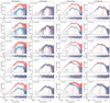 |
Fig. A.1. First and third columns: PS in two energy bands of NICER observations of MAXI J1820+070 covering the HSS-to-LHS transition. The 0.3 − 2 keV data are shown in blue while the 2 − 12 keV one is in red, both with the best-fitting model (solid line) consisting of a combination of Lorentzian functions (dotted lines). Second and fourth columns: Real and imaginary parts of the CS between the same two energy bands rotated by 45°. We plot Re cos(π/4)−Im sin(π/4) in blue and Re sin(π/4)+Im cos(π/4) in red, with the best-fitting model assuming the constant phase-lag model. In each panel, residuals with respect to the model, defined as Δχ = (data − model)/error, are also plotted. The dashed orange vertical line in each panel corresponds to the centroid frequency of the real/imaginary QPO in the model. |
Appendix A: rms and phase-lag energy spectra
In Fig. B.1, we show the rms and phase-lag energy spectra of the real/imaginary QPO for all the observations in the HSS-to-LHS transition of MAXI J1820+070. To produce these spectra, we extract the PS in six energy bands, 0.3 − 1.0, 1.0 − 1.5, 1.5 − 2.5, 2.5 − 4.0, 4.0 − 5.0, 5.0 − 12.0 keV, and we fit each of them simultaneously with the PS in the full energy band, 0.3 − 12 keV, and the CS between each narrow band and the full energy band. For each observation, we use the corresponding best-fitting model presented in Appendix A, with the centroid frequency and FWHM of every Lorentzian component fixed. We use the full energy band as the reference band for the phase-lags.
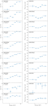 |
Fig. B.1. rms (left panels) and phase-lag (right panels) energy spectra of the real/imaginary QPO for the NICER observations of MAXI J1820+070 in the HSS-to-LHS transition. Horizontal lines cover the range of the energy band corresponding to each marker. |
All Tables
Best-fitting values of the QPO in MAXI J1820+070 for each observation with their corresponding 1-σ uncertainties.
Best-fitting parameters of the NICER observations of MAXI J1820+070 covering the HSS-to-LHS transition, and their corresponding 1 − σ uncertainties.
All Figures
|
Fig. 1. NICER X-ray light curve (left panel) and hardness-intensity diagram (right panel) of MAXI J1820+070 during its 2018 outburst. The intensity in both panels is the count rate per detector in the 0.5 − 12 keV band, while the hardness ratio in the right panel is the ratio of the count rates in the 2 − 12 keV to that in 0.5 − 12 keV. Each point corresponds to one obsID within 1200120101 − 1200120293. Light blue diamonds (obsIDs 1200120263 − 1200120265) and blue dots (obsIDs 1200120266 − 1200120270) depict the observations considered in this paper, in particular, the second ones correspond to those presenting narrow features in the phase lags and the coherence function. The orange star represents the observation 1200120197 studied by Ma et al. (2023), which covered the transition of type-C to a type-B QPO. |
| In the text | |
|
Fig. 2. Phase lags (left panels) and intrinsic coherence function (right panels) for NICER observations from 1200120263 to 120012070 of MAXI J1820+070 for the 0.3–2 keV and 2–12 keV energy bands. With a dashed red line, we depict the frequency of the imaginary QPO in each observation derived from the multi-Lorentzian fitting approach (see Sect. 4.1 for details). |
| In the text | |
|
Fig. 3. Top left panel: PS of NICER observation 1200120268 of MAXI J1820+070 in two energy bands. The 0.3–2 keV data are shown in blue while the 2–12 keV one is in red, both with the best-fitting model (solid line) consisting of 5 Lorentzian functions (dotted lines). Top right panel: real and imaginary parts of the CS between the same two energy bands rotated by 45°. We plot Re cos(π/4)−Im sin(π/4) in blue and Re sin(π/4)+Im cos(π/4) in red, with the best-fitting model assuming constant phase lags. Bottom panels: Phase-lag spectrum (left) and intrinsic coherence function (right) with the derived model (solid line) obtained from the fit to the PS and CS. In all four panels, residuals with respect to the model, defined as Δχ = (data − model)/error, are also plotted. The dashed orange vertical line at 2.06 Hz in every panel corresponds to the centroid frequency of the imaginary QPO in the model. |
| In the text | |
|
Fig. 4. Left panel: PS of NICER observation 1200120265 of MAXI J1820+070 in two energy bands. The 0.3 − 2 keV data are shown in blue while the 2 − 12 keV one is in red, both with the best-fitting model (solid line) consisting of 5 Lorentzian functions (dotted lines). Right panel: Real and imaginary parts of the CS between the same two energy bands rotated by 45°. We plot Re cos(π/4)−Im sin(π/4) in blue and Re sin(π/4)+Im cos(π/4) in red, with the best-fitting model assuming constant phase lags. In both panels, residuals with respect to the model, defined as Δχ = (data − model)/error, are also plotted. The dashed orange vertical line at 6.03 Hz in each panel corresponds to the centroid frequency of the QPO in the model. |
| In the text | |
|
Fig. 5. Evolution of the rms amplitude of the QPO in the 2.0 − 12.0 keV band (top left) and in the 0.3 − 2.0 keV band (bottom left) as MAXI J1820+070 transitions out of the HSS. The right panel displays the evolution of the phase lags of the QPO for the 2.0 − 12.0 keV band with respect to the 0.3 − 2.0 keV band. The rms and phase lags are derived from the fitted Lorentzian in our model (see Sect. 3). In the three panels, the horizontal bars correspond to the time duration of each observation, while the vertical bars are the actual 1 − σ errors of each quantity. The colour gradient depicts the centroid frequency of the QPO. |
| In the text | |
|
Fig. 6. Total fractional rms in the 0.3–12 keV band integrated from 0.1 to 50 Hz versus the centroid frequency of the QPO in MAXI J1820+070 (blue), with both quantities derived from our fitted model. Diamonds correspond to observations 1200120263-1200120265 while dots correspond to observations 1200120266_p1-1200120270. Green triangles and orange squares depict the type B and C QPOs identified in each orbit of observation 1200120197, which covered the HIMS-SIMS transition, studied by Ma et al. (2023). The solid and dashed lines connect the QPOs during the source hardening and softening respectively. Arrows indicate the direction of time progression in each sequence. |
| In the text | |
|
Fig. 7. rms (left panels) and phase-lag (right panels) spectra of the real/imaginary (blue circles), type-B (orange squares) and type-C (green triangles) QPOs in MAXI J1820+070. From top to bottom, the panels correspond to observations 1200120264_p2, 1200120265, 1200120266_p1 and 1200120266_p2 of MAXI J1820+070. The real and imaginary QPOs are from this work, while the type B and C QPOs are from observation 1200120197 analysed by Ma et al. (2023). For the comparison, we selected type-B and C QPOs with centroid frequencies most similar to those of the real/imaginary QPOs. Horizontal lines cover the range of the energy band corresponding to each marker. |
| In the text | |
|
Fig. A.1. First and third columns: PS in two energy bands of NICER observations of MAXI J1820+070 covering the HSS-to-LHS transition. The 0.3 − 2 keV data are shown in blue while the 2 − 12 keV one is in red, both with the best-fitting model (solid line) consisting of a combination of Lorentzian functions (dotted lines). Second and fourth columns: Real and imaginary parts of the CS between the same two energy bands rotated by 45°. We plot Re cos(π/4)−Im sin(π/4) in blue and Re sin(π/4)+Im cos(π/4) in red, with the best-fitting model assuming the constant phase-lag model. In each panel, residuals with respect to the model, defined as Δχ = (data − model)/error, are also plotted. The dashed orange vertical line in each panel corresponds to the centroid frequency of the real/imaginary QPO in the model. |
| In the text | |
|
Fig. B.1. rms (left panels) and phase-lag (right panels) energy spectra of the real/imaginary QPO for the NICER observations of MAXI J1820+070 in the HSS-to-LHS transition. Horizontal lines cover the range of the energy band corresponding to each marker. |
| In the text | |
Current usage metrics show cumulative count of Article Views (full-text article views including HTML views, PDF and ePub downloads, according to the available data) and Abstracts Views on Vision4Press platform.
Data correspond to usage on the plateform after 2015. The current usage metrics is available 48-96 hours after online publication and is updated daily on week days.
Initial download of the metrics may take a while.