| Issue |
A&A
Volume 696, April 2025
|
|
|---|---|---|
| Article Number | A237 | |
| Number of page(s) | 15 | |
| Section | Astrophysical processes | |
| DOI | https://doi.org/10.1051/0004-6361/202453523 | |
| Published online | 29 April 2025 | |
A hidden quasi-periodic oscillation in Cygnus X-1 revealed by NICER
1
Instituto Argentino de Radioastronomía (CCT La Plata, CONICET; CICPBA; UNLP), C.C.5, (1894), Villa Elisa, Argentina
2
Kapteyn Astronomical Institute, University of Groningen, PO Box 800 9700 AV Groningen, The Netherlands
3
Center for Astrophysics | Harvard & Smithsonian, 60 Garden Street, Cambridge, MA 02138, USA
4
Dr. Karl Remeis-Observatory and Erlangen Centre for Astroparticle Physics, Universität Erlangen-Nürnberg, Sternwartstr. 7, 96049 Bamberg, Germany
⋆ Corresponding author: This email address is being protected from spambots. You need JavaScript enabled to view it.
Received:
19
December
2024
Accepted:
28
February
2025
Abstract
Context. Cygnus X-1 is a high-mass black hole binary system that has been extensively studied across multiple wavelengths since its discovery in 1964. Its rapid temporal and spectral variability in X-rays offer critical insights into the physics of accretion and the dynamics around black hole systems. The power spectra of Cygnus X-1 are generally featureless and often modelled with two broad Lorentzian functions without the need for narrow quasi-periodic oscillations, which are prevalent in other black hole X-ray binaries.
Aims. We explore this phenomenon in light of the recent proposal that some variability components that are not detected in the power spectra may be significantly detected in the imaginary part of the cross spectra between two different energy bands and the coherence function. Specifically, we study the power, cross, and lag spectra and the coherence function of all available observations of Cygnus X-1 from the NICER mission up to Cycle 6 while looking for the so-called imaginary components.
Methods. We simultaneously fitted the power spectra of the source in two energy bands, 0.3−2 keV and 2−12 keV, and the real and imaginary parts of the cross spectrum between the same energy bands with a multi-Lorentzian model. Under the assumption that each Lorentzian is coherent between the two energy bands while the Lorentzians are incoherent with one another, our fits predict the intrinsic coherence and phase lags.
Results. The intrinsic coherence shows a narrow dip at a frequency that increases from ∼1 Hz to ∼6 Hz as the power-law index of the Comptonized component increases from ∼1.8 to ∼2.4. Simultaneously, the phase lags show a sudden and steep increase (hereafter referred to as the cliff) at the same frequencies. The dip and the cliff disappear if we use energy bands similar to those of the Rossi X-ray Timing Explorer mission (e.g. 3−5 keV and 5−12 keV) to compute the coherence and phase-lag spectrum. A narrow Lorentzian component with a low fractional root mean square amplitude and a large phase lag is required to effectively reproduce the drop of the intrinsic coherence. The rms and phase-lag spectra of this component change in a systematic way as the source moves in the hardness-intensity diagram.
Conclusions. This component, referred to as the imaginary QPO, exhibits behaviour consistent with the canonical type-C QPO despite being undetectable in the power spectra alone. Comparison with a similar QPO found in MAXI J1348–630 and MAXI J1820+070 further supports this identification. If our interpretation is correct, this would be the first time that the type-C QPO is detected in Cygnus X-1.
Key words: accretion / accretion disks / black hole physics / X-rays: individuals: Cygnus X-1
© The Authors 2025
 Open Access article, published by EDP Sciences, under the terms of the Creative Commons Attribution License (https://creativecommons.org/licenses/by/4.0), which permits unrestricted use, distribution, and reproduction in any medium, provided the original work is properly cited.
This article is published in open access under the Subscribe to Open model. This email address is being protected from spambots. You need JavaScript enabled to view it. to support open access publication.
1. Introduction
Accreting black hole binaries (BHBs) exhibit rich phenomenology in their X-ray light curves, with variability occurring over a wide range of timescales, from milliseconds to years (see e.g. the reviews by Belloni & Stella 2014; Belloni & Motta 2016; Ingram & Motta 2019). These sources display different spectral states, namely, the soft state, where the X-ray emission is dominated by thermal radiation from the accretion disc (Shakura & Sunyaev 1973), and the hard state, where inverse Compton scattering of soft photons by a hot plasma, or corona, dominates the energy spectrum (Sunyaev & Titarchuk 1980; Wilms et al. 2000). Intermediate states, known as hard- and soft-intermediate states, show characteristics of both regimes (Belloni et al. 2011). Each state is characterised by unique timing and spectral properties, with radio emission detected in the hard state and the hard- and soft-intermediate states but suppressed in the high-soft state (Fender et al. 2009). We note that for historic reasons, the ‘soft state’ in Cygnus X-1 is not the same as the high-soft state in transient low mass X-ray binaries. For a comparison between the hardness-intensity diagram (HID) of Cygnus X-1 and other transient systems, we refer to Figure 1 of König et al. (2024).
In an HID, transient BHBs follow a q-shaped trajectory that maps out the different spectral states, with transitions between states often accompanied by significant changes in jet activity. Specifically, the transition from the hard-intermediate to the soft-intermediate state, referred to as the jet line, is associated with discrete radio ejection events (Fender et al. 2009). This q-track behaviour is seen in other accreting systems, such as neutron star (NS) X-ray binaries, suggesting that fundamental accretion physics is at work in a wide range of objects (Motta et al. 2017).
Cygnus X-1, one of the most studied black hole binaries, is a persistent high-mass X-ray binary (HMXB) that accretes from the stellar wind of the supergiant HDE 226868 (Walborn 1973). Hosting a 21.2 ± 2.2 M⊙ black hole (Miller-Jones et al. 2021), Cygnus X-1 is key to understanding accretion physics and jet launching processes. It exhibits frequent state transitions, which are sometimes very rapid, crossing the jet line in the intermediate states (Pottschmidt et al. 2003). The system is characterised by a relatively small bolometric luminosity variation of a factor of three to four between states, and it never fully enters the disc-dominated regime (Wilms et al. 2006). Despite being constrained to the lower branch of the q-track (König et al. 2024), Cygnus X-1 shows rich multi-wavelength variability, including a radio jet during its hard state and polarised emission at high energies (Krawczynski et al. 2022; Chattopadhyay et al. 2023; Jana & Chang 2023).
The timing properties of BHBs can be investigated through Fourier analysis, where power density spectra (PDS) provide insights into the variability components (van der Klis 1989). These PDS reveal broadband variability extending up to 100 Hz along with narrow peaks corresponding to quasi-periodic oscillations (QPOs; Nowak 2000; Belloni et al. 2002). Low-frequency QPOs (LFQPOs), with frequencies from a few megahertz to ∼30 Hz, are commonly observed in BHBs and are classified into three types (A, B, and C) based on their quality factor1, fractional rms amplitude, phase lags, and the strength of the underlying noise (Casella et al. 2005). High-frequency QPOs, up to ∼350 Hz, are rarer, but their presence and characteristics suggest a link to similar oscillations seen in neutron star systems, implying a shared origin (Titarchuk et al. 1998; Belloni et al. 2012; Méndez et al. 2013).
The rms amplitude of PDS components, particularly the 0.1 − 10 Hz integrated rms amplitude, serves as a tracer of accretion regimes in BHBs (Belloni et al. 2011). The rms amplitude of QPOs tends to increase with energy, flattening above 10 keV, either increasing or decreasing at higher energies (Yan et al. 2018; Zhang et al. 2020; Yang et al. 2024; Zhu & Wang 2024). On the other hand, phase lags, which describe the delay between correlated light curves in two different energy bands, provide vital information about the variability components in the PDS at specific frequencies (Belloni et al. 2002; Muñoz-Darias et al. 2011). These lags can increase, decrease, or remain constant with energy, depending on the system and the characteristic frequency of the variability components (Reig et al. 2000; Zhang et al. 2020).
In the case of Cygnus X-1, the hard state PDS is commonly modelled using a combination of Lorentzian components (Nowak 2000), with rms variability reaching 30 − 40% in the 2 − 13 keV range (Pottschmidt et al. 2003). As the source transitions into the soft state, the rms drops to 10 − 20% (Grinberg et al. 2014; König et al. 2024), and the PDS becomes dominated by red noise (i.e. a power law). Time lag measurements in Cygnus X-1 have revealed a complex behaviour, whose interpretation is further complicated by the possibility of contributions from processes such as reprocessing in the accretion disc or scattering in the stellar wind (Grinberg et al. 2014; Lai et al. 2022; Härer et al. 2023; König et al. 2024).
Additionally, the coherence function, which measures the correlation between variability in different energy bands (Vaughan & Nowak 1997), offers further insight into the accretion dynamics. In some systems, such as MAXI J1348−630, MAXI J1820+070, and Cygnus X-1, the coherence drops at specific frequencies, and this drop is accompanied by a sudden increase of the phase lags (Nowak et al. 1999; Ji et al. 2003; König et al. 2024; Alabarta et al. 2024). It has been proposed (König et al. 2024) that the drop of the intrinsic coherence could be due to the ‘beat’ of two or more dominant variability components. The drop would then happen at the frequency difference between the two variability components, which can then produce a modulation in the observed variability when the components are sufficiently coupled. Another way the intrinsic coherence can drop at a specific frequency is if two or more components with different amplitudes and phases of their cross vectors contribute to the variability over the same frequency range (Vaughan & Nowak 1997; Méndez et al. 2024).
In this study, we leverage the high throughput and precise timing capabilities of the Neutron star Interior Composition ExploreR (NICER) to explore the broadband variability of Cygnus X-1 across its full range of observed spectral states, utilising data from several observing cycles. The structure of this paper is as follows: In Sect. 2 we present the NICER observations and data reduction processes. In Sect. 3 we outline the timing analysis, emphasising the variability components across distinct accretion states. Finally, in Sect. 4, we discuss our findings on Cygnus X-1 and compare them with other sources that have shown a similar behaviour.
2. Data analysis
The Neutron star Interior Composition ExploreR (Gendreau et al. 2016) is an instrument on board the International Space Station. NICER’s X-ray Timing Instrument (XTI) detector is sensitive to X-rays in the 0.3 − 12 keV energy range and has a temporal resolution of 40 ns. We analysed all available NICER archival observations of Cygnus X-1 up to Cycle 6, which consist of more than 100 pointings performed between June 2017 and June 2023, with exposures ranging from ∼0.1 to ∼30 ks. We used the NICER reduction tool nicerl2 from the HEASoft v.6.33.1 package with CALDB version xti20240206 to process the data. To filter out events that could contaminate the light curves, we selected events with an undershoot rate less than 200 counts s−1, an overshoot rate less than five counts s−1, and a cut-off rigidity (COR_SAX) greater than 1.5 GeV counts−1. Energy spectra were extracted using the nicerl3-spect routine with the Space Weather background model and a minimum of 30 counts per bin. We used XSPEC v12.14.0h (Arnaud 1996) to model each spectrum and extracted fluxes using the CFLUX convolution model.
We computed PDS from cleaned event files with the GHATS software2, using time segments of 128 s and a Nyquist frequency of 1024 Hz. We subtracted the contribution of the Poisson noise from the PDS (Zhang et al. 1995), which we estimated from the average of powers above 500 Hz, and normalised the PDS to units of root mean square squared per hertz (rms2 Hz−1). When converting the PDS to rms units, we did not apply a background correction since, compared to the source, the background count rate is negligible in all observations.
We defined three energy bands for the extraction of light curves and Fourier products: 0.3−12 keV (total), 0.3−2 keV (soft), and 2−12 keV (hard). Real and imaginary parts of the cross spectra (CS), phase lags, and intrinsic coherence were extracted using the formulae described in Méndez et al. (2024). To account for the partial correlation of photons simultaneously present in the narrow and total energy bands, we subtracted the average of the real part of the CS calculated over a frequency range where the source has no contribution. We applied a logarithmic rebin to all Fourier products such that the size of each frequency bin increases by 101/100 with respect to the previous one. Finally, we simultaneously fitted the soft and hard PDS as well as the rotated3 real and imaginary parts of the CS using XSPEC v.12.14.0h (Arnaud 1996) from ∼0.004 Hz up to 200 Hz.
In Table B.1, we show the complete NICER dataset used in this work. The reported exposure times correspond to the sum of the total non-zero GTIs created by GHATS after processing the cleaned event files.
3. Results
3.1. Constructing an absorption corrected HID
To analyse the entire NICER dataset, we first constructed the HID using unabsorbed fluxes for the same energy bands and time segments used to create the power spectra. For this, we fitted the energy spectrum of each 128 s segment in the 0.3−12 keV energy range with the model TBABS×(DISKBB+POWERLAW) to account for the thermal emission of the accretion disc and the Comptonized emission of the corona, as both are affected by interstellar absorption. We used a power law instead of a Comptonization model to facilitate the comparison with previous studies (see e.g. Done et al. 1992; Di Salvo et al. 2001; Zdziarski et al. 2002; Wilms et al. 2006). For the TBABS component, we used the cross-section tables of Verner et al. (1996) and the abundances of Wilms et al. (2000). We applied a 5% systematic error, which is higher than the recommended value, to account for our use of a simplified spectral model (a disc plus a Comptonizing corona) that excludes broad emission lines, relativistic reflection, and non-solar interstellar medium abundances. Following the approach of König et al. (2024), this method enables the construction of an HID based on intrinsic source fluxes, minimising the impact of interstellar absorption.
We excluded segments that yielded reduced χ2 greater than two, which mostly correspond to intervals of high absorption (NH > 0.7 × 1022 cm−2), low or high disc temperatures (kTdbb < 0.1 keV or kTdbb > 0.5 keV), and a low or high spectral index (Γ < 1.4 or Γ > 3.4). These excluded segments are most likely affected by the stellar wind of the companion (Wilms et al. 2006). After all the filtering, we kept 92.7% of the original set of segments of 128 s, corresponding to a total of ∼380 ks of NICER data across the entire HID, as displayed in Fig. 1.
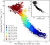 |
Fig. 1. Hardness-intensity diagram computed from the unabsorbed fluxes of the NICER dataset of Cygnus X-1. The hardness ratio in x axis is defined as the ratio of the unabsorbed flux in the 2 − 12 keV band to that in 0.3 − 2 keV band, while the y axis is the unabsorbed flux in the 0.3 − 12 keV band. The fluxes were obtained from the fitting each 128 s segment with a model consisting of disc black body plus a power-law component, both affected by interstellar absorption. The different colours indicate the 10 distinct regions we use in this paper, parametrized by the increasing spectral index, Γ, of the power-law component (see legend). The grey error bars in the main panel indicate the 1σ errors of the fluxes and hardness ratios. Top-right inset panel: HID of Cygnus X-1 computed from the observed count rates in the same energy bands as in the main panel; the black points correspond to the segments we used in this work, whereas the grey points are the segments that we discarded in our analysis (see text for details). |
In the same figure, we include the instrument-dependent HID for comparison, and we distinguish the time segments that we retained (black) from the segments that we discarded (gray). We note that the hardness ratio in both cases spans about a decade, the 0.3−12 keV intensity spans almost two orders of magnitude, and the unabsorbed 0.3−12 keV flux changes by a factor of ∼30.
We segmented the HID by the power-law spectral index in bins of width ΔΓ = 0.1, starting at the low-hard state (Γ ≃ 1.4) and finishing at the softest state registered (Γ ≃ 3.4). After visually inspecting and comparing the frequency-dependent phase lags and intrinsic coherence of each bin, we combined the data to form ten distinct regions, Z1 to Z10, across the HID. These regions are colour coded in Fig. 1, where we indicate the corresponding values of the spectral index. Using the same colour scheme, we present in Fig. 2 the phase lags and coherence function between the 0.3−2 keV and 2−12 keV energy band of each region.
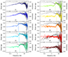 |
Fig. 2. Phase lags in radians (colour points) and intrinsic coherence (gray points) of each region of the HID of Cygnus X-1 restricted to frequencies between 0.02 Hz and 30 Hz. The vertical stripe indicates the minimum of the coherence drop and the maximum of the cliff of the phase lags. The phase lags and coherence are computed between 0.3−2 keV and 2−12 keV energy bands, with the latter used as a reference band. |
Properties of the defined HID regions.
The most prominent feature seen in Fig. 2 (and the main focus of this work) is the appearance of a sudden and steep increase in phase lags in conjunction with a sudden drop in the coherence (see König et al. 2024)4. These two features appear to correlate with frequency and spectral hardness, as the frequency at which they appear shifts from ∼1.5 Hz in Z3 (Γ ≃ 1.8, the first HID region where it appears) up to ∼6 Hz in Z8 (Γ ≃ 2.4). In Fig. 2, we mark the centroid frequency of the coherence drop using a vertical stripe, which was derived from modelling the Fourier products, as we describe in Sect. 3.3.
To identify more precisely the value of the photon index at which the cliff and drop features appear, we segmented the HID around Z2 and Z3 by spectral index in bins of size ΔΓ = 0.05. We find that the feature appears rather abruptly at Γ ≃ 1.8 at a frequency of approximately 1 Hz.
3.2. Dependence of the coherence drop upon energy
Cygnus X-1 has been observed repeatedly since its discovery in 1964. For instance, the Rossi X-ray Timing Explorer (RXTE) mission has accumulated close to 4.8 Ms in exposure time across several observing campaigns (e.g. Belloni et al. 1996; Revnivtsev et al. 2000; Grinberg et al. 2014). However, the drop and cliff features presented here have not been reported before until the appearance of NICER. As noted by König et al. (2024), the key difference is the data at energies below 3 keV, which RXTE could not cover.
To illustrate this, in Fig. 3 we show the phase lags and intrinsic coherence of region Z3 but computed from energy bands similar to those commonly used with RXTE data: 3−5 keV and 5−12 keV. It is apparent in this figure that neither the cliff feature in the phase lags nor the drop feature in the coherence are present. As shown in Figure 8 of König et al. (2024), the feature in the coherence function appeared only when they considered a band below ∼1.5−2 keV.
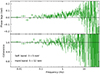 |
Fig. 3. Phase lags and intrinsic coherence function of region Z3 of the HID of Cygnus X-1 computed between the 3−5 keV and 5−12 keV energy bands. No evidence of the coherence drop or the cliff of the phase lags at ∼1.5 Hz is apparent (see Fig. 2). The horizontal lines in each panel indicate the reference levels for zero phase lag and unity coherence, respectively. |
3.3. Constant phase-lag model
Following Méndez et al. (2024), we used XSPEC to simultaneously fit the PDS in two energy bands (0.3−2 keV and 2−12 keV) as well as the real and imaginary parts of the cross spectrum in the same two bands. At all Fourier frequencies, the magnitude of the real part of the cross spectrum is consistently larger than the magnitude of the imaginary part. To improve the stability of the fitting procedures, such as the Levenberg–Marquardt algorithm in XSPEC, which work more effectively when parameters are of similar magnitude, we rotated the cross vectors by 45°5. This rotation equalized the real and imaginary components for cross vectors with zero phase lag without altering the modulus or the fit parameters. In the following figures, we present the rotated components  and
and  , which remain positive and enable the use of logarithmic axes. Phase lags are reported after subtracting π/4, returning the values to the reference frame of the original non-rotated cross vector.
The PDS in the two bands were modelled using Lorentzian functions, with the centroid frequency and width of each Lorentzian tied across all Fourier products. To model the CS components, we applied two different variants: a constant phase-lag model and a constant time-lag model. Each model assumes that the phase lags of each Lorentzian component are either independent of frequency (constant phase-lag model, hereafter ϕ model) or linearly dependent upon frequency (constant time-lag model, hereafter τ-model). To keep the analysis as straightforward as possible, we adopted the ϕ model in the main text. However, we also fitted the data using the τ-model, and the corresponding results are presented in Appendix A.
Each Lorentzian component in the cross spectrum was then multiplied by the cosine (real part) or sine (imaginary part) of the phase-lag model. Thus, each Lorentzian model has a total of six free parameters across all four Fourier components: centroid frequency and width, soft and hard PDS normalisations, phase lag and CS normalisation.
Each region of the HID is described with a variable number of Lorentzians. We considered that a Lorentzian component is significant if at least one of the three free normalisations is not consistent with zero at the 3σ level. As noted by Méndez et al. (2024), if each Lorentzian is perfectly coherent in the two energy bands, the normalisation C of each Lorentzian in the CS can be written in terms of the normalisations of the soft (Ns) and hard (Nh) PDS normalisations as C = (NsNh)1/2. Here, we did not link these parameters during the fit, but we checked that after the fit, this relationship held for all components within uncertainties.
The best-fitting parameters as well as the 1σ uncertainties were derived from Markov chain Monte Carlo simulations using the XSPEC CHAIN command. We verified that each chain converged correctly by visually inspecting each parameter trace plot and by simultaneously verifying that the autocorrelation time is close to unity6. To achieve this, we constructed MCMC chains of length 106, and by burning the first 5 × 10⁵ steps. In Tables C.1 and C.2, we present a summary of the entire set of properties of the Lorentzian components used to model the ten regions of the HID respectively with the constant phase-lag and the constant time-lag models.
Best-fit statistics summary.
To better visualise the entire collection of Lorentzian components and their respective properties shown in Table C.1, we constructed bubble plots. Figure 4 displays the characteristic frequency of each Lorentzian (horizontal axis), defined as (ν02 + Δ2)1/2, where ν0 and Δ are the centroid frequency and full width at half maximum of the corresponding Lorentzian (Belloni & Bhattacharya 2022). On the vertical axis, we display each HID region (increasing upwards). The bubble area is proportional to the rms amplitude of the cross vector, also known as the covariance amplitude. A colour map is used to display phase lags (in radians). In Table 2, we show the total χ2 and degrees of freedom corresponding to each HID region and applied model as well as the number of Lorentzians used per region and model.
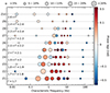 |
Fig. 4. Bubble plot of every Lorentzian in each HID region (vertical axis) of Cygnus X-1 as a function of their characteristic frequency (horizontal axis). The area of each bubble is proportional to the covariance rms amplitude of the Lorentzian. The colour scheme indicates the corresponding phase lag. The diamond marker highlights the narrow QPO responsible for the sharp coherence drop, which becomes apparent in Zones 3 to 8, corresponding to intermediate states with 1.8 < Γ < 2.4. |
The entire collection of soft and hard PDS as well as the rotated real and imaginary parts of the CS of Cygnus X-1, between ∼0.004 and 200 Hz (approximately five decades in frequency), can generally be described with about six broad Lorentzians with a quality factor Q ≲ 0.5, while the relative contributions to the total rms vary according to the spectral hardness of the source. This description of about six broad components is most notably seen in the hardest low-flux observations (Γ < 1.8) and the softest high-flux observations (Γ > 2.4). In the observations at intermediate hardness (1.8 < Γ < 2.4), we noticed that to simultaneously fit the PDS and CSs correctly, we needed to add extra narrow components (Q > 0.5), specifically between 1 and 10 Hz.
The necessity to add narrow Lorentzian components to adequately model the Fourier products may arise from the combination of various factors. First and foremost, NICER’s high throughput and low energy coverage may reveal components that up to now were undetectable with previous less sensitive missions or missions not covering the same energy band. Moreover, we achieved a great signal to noise ratio in each HID region by averaging several segments (see Table 2) and by afterwards logarithmically rebinning each Fourier product. Secondly, the simultaneous PDS and CS modelling utilised here can reveal weak or hidden variability components that may otherwise be lost by fitting only the PDS (Méndez et al. 2024).
When looking at the evolution of all the Lorentzian components across the HID in Fig. 4, a clear shift towards higher frequencies can be seen as the source spectrum softens. For example, the Lorentzian that in the hardest region (Z1) starts at ∼0.3 Hz with ≳20% rms ends up in region Z8 at ∼2 Hz with ≲10% rms. This is the component at the lowest frequency out of the two broad components historically used to model the PDS in the hard state of Cygnus X-1 (see e.g. Pottschmidt et al. 2003). This phenomenon of increasing frequency shift accompanied by a decreasing rms is seen in almost all components in the regions between Z1 and Z8. In regions Z9 and Z10, where Γ > 2.4, the PDS show the typical power-law shape studied extensively in previous campaigns of Cygnus X-1 (Pottschmidt et al. 2003).
The PDS and CS of Cygnus X-1 also show one broad (Q ≲ 0.1) Lorentzian component at a very low frequency that remains between 0.01 Hz and 0.02 Hz across the entire HID, with the rms close to 5% except in the very soft regions where it reaches ∼10%. Only in regions Z4 and Z5 (1.9 < Γ < 2.1) was this component not significant enough for it to be fitted properly. These components display small phase lags (|Δϕ|≲0.01), as shown in white in Fig. 4.
Finally, we note in Fig. 4 the significant detection of a high frequency (HF) component both in the PDS and CS at frequencies above 50 Hz in the hardest region (Γ ≃ 1.4), reaching up to ∼150 Hz in region Z8 (Γ ≃ 2.4). This HF component is quite broad (Q ∼ 0.5) and weak (rms ∼ 5%), with large negative phase lags (close to 1 rad). We analyse this HF component further in Sect. 3.7.
The low frequency and HF components can be seen in Fig. 5. On the left side of each plot, we show the soft and hard PDS as well as the rotated real and imaginary parts of the CS of region Z3 (1.8 < Γ < 1.9). On the right hand side of each plot, we show the phase lags and intrinsic coherence together with their respective derived models. This region was successfully modelled using ten Lorentzians, yielding a χ2 of 1148.8 for 1140 degrees of freedom. The residuals show some structure, but the addition of more Lorentzian components did not improve the fit. The Lorentzian component responsible for the coherence drop seen in this figure is shown with a thicker line. This highlighted component of region Z3 corresponds to the Lorentzian shown with a diamond marker in Fig. 4.
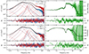 |
Fig. 5. Constant phase-lag model applied to region Z3 of the HID of Cygnus X-1. The top-left panels show the soft (0.3 − 2 keV) and hard (2 − 12 keV) PDS in rms2 units and residuals. The bottom-left panels show the real and imaginary parts of the cross spectrum (with the cross vector rotated by π/4) in rms2 units and the residuals. The top-right panels show the phase lags (rad) with the derived model and residuals. The bottom-right panels show the intrinsic coherence with the derived model and residuals. As described in the text, the model lines drawn in the right panels have not been fitted to the phase lags and the coherence but have been derived from the fits to the PDS and CS in the left panels. The QPO responsible for the coherence drop is highlighted over the other Lorentzians using a thicker line (at ν ∼ 1.3 Hz). The solid lines in the plots of the phase lags and coherence function show the derived model of those two quantities for ten Lorentzians (see text). Because the total phase lag spectrum and coherence function are not a combination of additive components, in these plots we cannot show the contribution of each Lorentzian. To show the effect of the imaginary QPO, the dashed lines in the plots show the derived models without the Lorentzian associated with the Imaginary QPO (without refitting the data). |
3.4. Frequency dependence of the intrinsic coherence and phase lags
In Fig. 4, the diamond marker shows the Lorentzian component that coincides with (and which we attribute to) the coherence drop. This component can be traced from region Z3 at ∼1.5 Hz up to region Z8, reaching ∼6 Hz. Although Fig. 2 shows that in region Z2 there is a slight coherence drop at ∼1 Hz, we could not adequately constrain any narrow component in this region. Figure 4 also shows that the phase lag of the highlighted component varies between 0.2 rad and 0.5 rad from regions Z3 to Z7 and then decreases below 0.1 rad in region Z8. The covariance rms amplitude of that component remains below 5% in all six regions where it is detected, with a quality factor above two (see Table C.1 for details).
An example of how this component fits in between stronger and broader ones can be seen in Fig. 5. We note that this component (highlighted using a thicker line) is most significantly detected in the imaginary part of the cross spectrum (hence the large phase lag), and the rms amplitudes (proportional to the root square of the normalisations in the PDS) in the soft and hard bands are very similar in magnitude. This behaviour is very different from that of the other Lorentzian components, and it shows that the hard dominates over the soft component by a few factors. This is the reason why we choose call the Lorentzian component that causes the cliff in the phase-lag spectrum and the drop in the coherence the imaginary QPO.
We tested the scenario shown in Fig. 5 without the inclusion of the imaginary QPO. This test yielded a χ2 of 1526.8 over 1146 degrees of freedom. For comparison, the best fit for region Z3 shown in Table 2 resulted in a χ2 of 1148.8 with 1140 degrees of freedom. Additionally, the residuals of the 0.3 − 2 keV PDS exhibited a 4σ structured excess around the frequency of the imaginary QPO at approximately ∼1.5 Hz. Similarly, the residuals of the imaginary part of the CS showed a 3σ structured excess at this frequency. Meanwhile, the residuals of the 2−12 keV PDS and the real part of the CS displayed a structured excess around the same frequency, close to 1σ, but it is not statistically significant. To show the contribution of the narrow imaginary QPO component to the phase-lag spectrum and the intrinsic coherence function, in the right panels of Fig. 5 we show with dashed lines the derived models without that component and without refitting the data.
3.5. Energy dependence of the amplitude and phase lags of the imaginary QPO
To analyse the rms energy spectrum of the imaginary QPO, we constructed the PDS of regions 3 to 8 in the following energy bands: 0.3−0.5 keV, 0.5−0.9 keV, 0.9−1.2 keV, 1.2−1.9 keV, 1.9−2.9 keV, 2.9−4.5 keV, 4.5−7 keV, and 7−12 keV. We used the full 0.3−12 keV energy band as a reference to compute the CS. We then fitted the full band PDS, the band specific PDS, and the real and imaginary parts of the CS of each region using XSPEC. The complete rms and phase-lag spectrum of the imaginary QPO for each region is presented in Fig. 6.
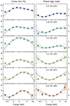 |
Fig. 6. Covariance rms amplitude (in percent, left column) and phase lags (radians, right panel) of the imaginary QPO that cause the coherence drop of Cygnus X-1 as a function of energy. The centroid frequency of the imaginary QPO is indicated in each panel. A cubic polynomial has been fitted in each case to track the corresponding minima or maxima. In each panel, we show cubic model realisations in grey that depict the 1σ confidence range of the fits. |
The rms spectrum of the imaginary QPO shows a wave-like structure across all six regions, and one or two local extrema can be identified in the 0.3−12 keV energy range. The main differences observed between regions are the average rms level and the energy where the rms peaks. There is no clear dependence of the average rms level on the spectral hardness, but there is an apparent systematic change of the rms peak energy with the spectral hardness. In region Z3 (Γ ≃ 1.8), the rms peaks at ∼1.5 keV, whereas in region Z8 (Γ ≃ 2.4), the rms maximum is at about ∼2.5 keV.
The phase-lag energy spectrum, on the other hand, shows an elongated U shape that evolves as the source moves in the HID. Interestingly, as the frequency of the imaginary QPO increases (softer regions), the location of the minimum moves to higher energies, and the U shape becomes more pronounced (less elongated), with values of the phase lags at very low and very high energies becoming increasingly positive (close to 1 radian). The U shape of the phase lags shown in Fig. 6 is consistent with the plot in the middle panel of Fig. 11 in König et al. (2024).
We fitted a cubic polynomial to find the maximum or minimum of the phase-lag and rms spectra, and in each case, we used Markov chain Monte Carlo simulations of 106 samples to estimate the uncertainties of these values. We report these values in Table 3. At this point, it became apparent that there is a positive relationship between the imaginary QPO frequency (νQPO) and the maximum of the rms spectrum and the minimum of the phase-lag spectrum. As νQPO increases from 1.5 Hz to 6 Hz, the energy at which the rms spectrum is at maximum increases from 1.9 keV to 3.5 keV, while the energy at which the lag spectrum is at minimum increases from 0.7 keV to 2 keV.
Energies of the rms and phase-lag extrema.
3.6. The structure of the ‘plateau’ in the phase-lag frequency spectrum
As noted by Vaughan & Nowak (1997), the coherence function can be less than unity if more than one region of the accretion flow contributes to the signal in two energy bands, even if each region produces perfectly coherent variability. Indeed, if the observed light curve consists of two signals, and each of them is perfectly coherent in two energy bands (i = 1, 2), the coherence is less than unity except if |Q1|/|Q2|=|R1|/|R2| and δθr = δθq, where Qi, Ri are the Fourier amplitudes of the two signals in the two bands and δθr and δθq are the phase lags of the signals between those same two bands.
As seen in Figs. 4 and 5, Lorentzians L6 and L7 of region Z3 (numbered by increasing characteristic frequency; see Table C.1 for details)7 have very similar ratios between the power spectra in the soft and hard energy bands (visual comparison) and very similar phase lags (∼0.2 rad). Specifically, we verified that the ratios Q1/Q2 × R2/R1 and δθr/δθq are all consistent with being one within 1σ. Here, Q1, 2 and R1, 2 respectively represent the normalisations of L6 and L7 in the two energy bands 0.3−2 keV and 2−12 keV band. All of this leads to a plateau8 in the lag frequency spectrum at frequencies just above that of the cliff.
Given the best-fit model of region Z3 shown in Table 1, we linked the normalisations and lags of components L6 and L7, and we obtained a total χ2 of 1149.3 for 1142 degrees of freedom. An F-test of the two fits yielded a null probability of 0.78, which indicates that a model with more free parameters is not favoured.
We therefore note that the underlying structure behind this plateau can be approximated by a combination of two or more Lorentzian profiles with similar phase lags and correlated normalisations of the power spectra in the two energy bands through the relationships described above. However, in the previous sections, and for the rest of this work, we leave all parameters of each Lorentzian free. In this section, we have shown that some variability components may not be well described by a Lorentzian function, as the linear combination of Lorentzian functions is not a Lorentzian function.
3.7. The high-frequency bump
As seen in Fig. 5, Cygnus X-1 shows statistically significant variability at high frequency, up to ∼200 Hz. This variability, which can be fitted with a Lorentzian function, is present across a large part of the HID, with the centroid frequency of the best-fitting Lorentzian ranging from ∼50 Hz in the hardest region Z1 (Γ ≃ 1.4) to ∼160 Hz in region Z8 (Γ ≃ 2.4). This component is broad, with a quality factor between 0.2 and 0.5, and has large negative phase lags of approximately −0.5 rad. As in previous work with sources such as GRS 1915+105 (Zhang et al. 2022) and GX 339−4 (Zhang et al. 2024), we call this high-frequency variability component the HF bump.
We computed the covariance rms amplitude and phase-lag spectrum of the HF bump across the eight regions of the HID in which the imaginary QPO is significantly detected, which we show in Fig. 7. In the same way as for the imaginary QPO, we fitted the covariance rms and phase-lag spectrum in each region with a cubic polynomial (black line) and plotted the 1σ uncertainty of the model as a grey shadow. Contrary to what we find for the imaginary QPO (Fig. 6), neither the covariance rms nor the phase lags show any clear minimum or maximum. The covariance rms amplitude of the HF bump does not exceed ∼5%. The energy dependent phase lags tend towards zero at energies above 1 keV and show small sign variations with no apparent pattern.
We note that the frequency of the HF bump (νbump) appears to follow a broken power-law relation with both the spectral index Γ and the frequency of the imaginary QPO (νQPO). This is depicted in the insets of Fig. 8. Following Zhang et al. (2022), we constructed a new variable x = νQPO + c ⋅ Γ, where c = cot(ϕ), with ϕ being the rotation angle of the νQPO and Γ as the axes around the axis of the frequency of the bump. The best fit of log νbump versus x yields c = 1.4, with a Pearson R2 coefficient of 0.96. The relationship between the characteristic frequencies of the imaginary QPO and the HF bump with spectral hardness may indicate that these components have the same physical origin.
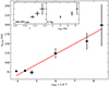 |
Fig. 8. Characteristic frequency of the high-frequency bump of Cygnus X-1 as a function of a linear combination of the spectral index, Γ, and the frequency of the imaginary QPO, νQPO. Top insets show the individual correlations. The best-fit linear model is shown in red. |
4. Discussion
We report the discovery of a previously undetected QPO in Cygnus X-1 that appears in intermediate spectral states of the source (1.8 < Γ < 2.4). This QPO is narrow (Q ≳ 2), with a large phase lag (∼0.3 rad), making it significant in the imaginary part of the cross spectrum but not in the power spectrum. Because of this, we call it the imaginary QPO. The centroid frequency of this QPO increases systematically from approximately ∼1.5 Hz to ∼6 Hz as Cygnus X-1 transitions to softer spectral states. The rms energy spectrum of the imaginary QPO reveals a rising trend at higher energies, with a maximum that shifts from ∼1.9 keV when Γ ≃ 1.8 to ∼3.5 keV when Γ ≃ 2.4. Additionally, the phase-lag energy spectrum exhibits a characteristic U shape, with a local minimum that shifts from ∼0.7 keV when Γ ≃ 1.8 (kTdbb ≃ 0.25 keV) to ∼2 keV when Γ ≃ 2.4 (kTdbb ≃ 0.35 keV). The centroid frequency of the imaginary QPO also correlates closely with the centroid frequency of a high-frequency bump present in the hard and hard-intermediate spectral states of Cygnus X-1.
Recently, König et al. (2024) reported a coherence drop and lag increase in the frequency range that lies between the two well-known broad Lorentzian components (e.g. Pottschmidt et al. 2003) in the power spectrum of Cygnus X-1 and other black hole binaries such as MAXI J1820+070 and MAXI J1348–630. König et al. (2024) suggests that these features could both be attributed to the beating between two broad Lorentzian components as well as an additional narrow Lorentzian component. The need of a narrow Lorentzian component with large positive phase lags to simultaneously fit the PDS and CS supports the alternative interpretation that this imaginary QPO is an independent feature rather than a beat between the two broad Lorentzians. The beat between two broad components does not produce such a sharp drop in the coherence function nor the steep rise in the phase lags This distinction is crucial for understanding the variability mechanisms in Cygnus X-1, as it indicates that multiple narrow components may dominate the broadband variability structure in this system, even in the absence of significant features in the power spectrum (Méndez et al. 2024).
We can compare our finding for Cygnus X-1 with the results from the study of MAXI J1820+070 (Méndez et al. 2024; see also Bellavita et al. 2025) and MAXI J1348–630 (Alabarta et al. 2024). Méndez et al. (2024) and Alabarta et al. (2024) demonstrated that while the respective PDS of MAXI J1820+070 and MAXI J1348–630 could be modelled with four broad Lorentzian components, the joint fitting of the PDS and CS required at least seven narrower Lorentzian functions. This emphasises that the variability in the cross spectrum can reveal hidden components that are not significantly detected in the power spectrum alone (Méndez et al. 2024). In these sources, the coherence drops when multiple Lorentzian components overlap in frequency, suggesting that the coherence function is sensitive to the detailed structure of the variability. In Cygnus X-1, we observed a similar effect, where the coherence drop and phase-lag cliff are linked to the presence of a narrow imaginary QPO component that is not significant in the PDS but is significantly detected in the CS.
The phase-lag and coherence spectra in Cygnus X-1 resemble those observed in MAXI J1348–630 during the decay of the 2019 outburst (Alabarta et al. 2024). Unlike in Cygnus X-1, where the imaginary QPO is only detected in the CS, the features in MAXI J1348–630 were associated with a significant Lorentzian both in the PDS and CS. In MAXI J1348–630, the sudden increase in the phase-lag spectrum (the cliff) and the narrow coherence drop happens at the same frequency as the type-C QPO, suggesting a direct link between the two features.
Our findings on the imaginary QPO in Cygnus X-1 align with known properties of type-C QPOs. The imaginary QPO appears only in hard-intermediate spectral states, spanning a frequency range from ∼1 Hz to ∼6 Hz, with a monotonic correlation between its frequency and the photon index of the Comptonizing component, Γ. The imaginary QPO also shows a rising rms energy trend, similar to type-C QPOs (see e.g. Alabarta et al. 2022; Ma et al. 2023; Rawat et al. 2023) and exhibits phase-lag energy spectra with a distinctive U shape. Specifically, the phase-lag minimum correlates with the disc black body temperature (kTdbb; see Tables 1 and 3), a behaviour consistent with predictions from the time-dependent Comptonization model vKompth (Karpouzas et al. 2021; García et al. 2021; Bellavita et al. 2022). These features, along with the results of Alabarta et al. (2024) in MAXI J1348–630, strongly suggest that the imaginary QPO in Cygnus X-1 is indeed a type-C QPO.
While a detailed application to Cygnus X-1 is beyond the scope of this paper, the observed phenomenology can still be interpreted within the framework of time-dependent Comptonization. In the vKompth model, soft photons from the accretion disc enter a spherical corona of hot electrons, undergoing inverse-Compton scattering and emerging with higher energies. Photons experiencing more scatterings escape later and at higher energies, producing hard lags. Conversely, if some up-scattered photons return to the disc, are reprocessed, and then re-emitted, this feedback mechanism introduces soft lags. The resulting phase-lag spectrum exhibits a characteristic U shape, with its minimum shifting to higher energies as the disc temperature increases (see Figure 2 of Bellavita et al. 2022). Our results in Tables 1 and 3 show that, as predicted by the model, the energy at which the U-shaped phase-lag spectrum of the imaginary QPO is minimum increases as the temperature of the DISKBB component increases. This suggests that the imaginary QPO could be due to the time-dependent Comptonization.
An interesting comparison can be drawn between the imaginary QPO observed in Cygnus X-1 and those seen in MAXI J1820+070 and MAXI J1348–630. In both cases, these sources exhibit QPOs that, in the PDS, are overshadowed by much stronger neighbouring variability components. This is in stark contrast to other black hole binaries, such as GRS 1915+105, GX 339–4, or Swift J1727.8–1613, where confirmed type-C QPOs are stronger and stand out clearly in the power spectrum (Zhang et al. 2017; Belloni et al. 2024; Mereminskiy et al. 2024). These stronger type-C QPOs, which are mainly observed in the high luminosity hard-to-soft transitions of an outburst, do not exhibit the coherence drop or the steep rise in phase lag that we observe in Cygnus X-1 and MAXI J1820+070. In contrast, the imaginary QPOs in MAXI J1820+070 and MAXI J1348–630 are observed in the soft-to-hard transition during the decay of the outburst. This coincides with the region in the HID spanned by Cygnus X-1 (König et al. 2024). The presence of this imaginary QPO not only in an HMXB-like Cygnus X-1 but also in other LMXBs suggests that this variability component, with its associated phase-lag and coherence features, are not dependent on the interaction of X-rays with the stellar wind of the companion and instead related to a phenomenon intrinsic to the accretion flow. We emphasise that the soft state of Cygnus X-1, even on a scaled HID (see Fig. 1 of König et al. 2024), does not coincide with the classical soft state of BH-LMXBs.
The fact that the same combination of Lorentzian functions that fits the PDS and CS can accurately predict the lag spectrum and the coherence function in Cygnus X-1 (this paper) and other sources (MAXI J1820+070, Méndez et al. 2024; Bellavita et al. 2025; MAXI J1348–630, Alabarta et al. 2024) further supports the proposal that each Lorentzian component has its own distinct phase-lag frequency spectrum. This idea challenges the view that broadband lags in X-ray binaries are due to a smooth global transfer function, such as in the case of reverberation (Ingram et al. 2009, 2019) and propagating fluctuations (Turner & Reynolds 2021; Mummery 2023). Instead, the variability in these systems may arise from multiple, separate resonances within the accretion flow, each contributing to the observed lags and coherence behaviour. Our results provide further support to this picture, suggesting that the imaginary QPO we have detected could be one of these distinct resonances, reflecting a complex interplay between the accretion disc and the Comptonizing corona. Furthermore, not every Lorenztian component used to model the PDS and CS should be linked to a separate resonance. We showed in Sect. 3.6 that in many cases individual Lorenztians could represent different manifestations of a single variability component (e.g. fundamental plus harmonics), thus reducing the total number of separate resonances.
The model of Méndez et al. (2024) assumes that each variability component is fully coherent across any two energy bands, while the different components themselves are mutually incoherent. Interestingly, the coherence drop in Cygnus X-1 is only observed when including data below 2 keV, suggesting that the two variability components that cause the drop of the coherence may be the corona and the accretion disc. This interpretation seems counterintuitive, as the disc provides seed photons for inverse Compton scattering in the corona, implying that variability in these two components should be correlated. One possible resolution to this apparent contradiction is if the disc variability responsible for the coherence drop arises from accretion rate fluctuations within the disc, which undergo viscous damping before reaching the corona (Wilkinson & Uttley 2009). Another possibility is that the low-energy variability is contributed by a component other than the disc.
Finally, we report, for the first time, a detailed analysis of the HF bump in Cygnus X-1 based on the capabilities of NICER. This HF component has been reported before using RXTE observations (see e.g. Belloni et al. 1996; Nowak et al. 1999; Revnivtsev et al. 2000) and is also apparent in the PDS in König et al. (2024), although they did not discuss it in detail. This component, with frequencies ranging from 50 Hz to 150 Hz, exhibits large negative phase lags and shares similarities with other HF bumps observed in other black hole binaries. The discovery of this high-frequency component further reinforces the idea that multiple distinct Lorentzian components, each with its own timing and phase-lag properties, contribute to the overall variability of Cygnus X-1. This component and the imaginary QPO share similar properties with the HF bump and the type-C QPO detected in GRS 1915+105 (Zhang et al. 2022). In both cases, the frequency of the HF bump is better correlated to a linear combination of the type-C QPO (the imaginary QPO in Cygnus X-1) and the spectral hardness (Γ in the case of Cygnus X-1) than to each of those quantities separately. This reinforces the interpretation that the imaginary QPO in Cygnus X-1 is the type-C QPO.
The quality factor Q of a Lorentzian profile is defined as ν0/Δ, where ν0 is the centroid frequency and Δ is the full width at half maximum.
As described in Méndez et al. (2024), π/4 radians are added to the argument of both components of the CS, which is appropriately accounted for afterwards when modelling.
From now on, ‘cliff’ refers to the phase lags’ feature, while ‘drop’ refers to the relative narrow feature in the coherence function.
See Section 15.5.2 of Press et al. (2007) for a discussion on the importance of the correct scaling of the Hessian matrix in the context of the Levenberg–Marquardt algorithm.
In this work, the classical broad components used to fit the PDS of Cygnus X-1 in the 0.1−10 Hz frequency range, L1 and L2 (see e.g. Pottschmidt et al. 2003; Grinberg et al. 2014; König et al. 2024), correspond to the combination of, respectively, Lorentzians L3 + L4 and L6 + L7.
In geological terms, a plateau is an area of flat terrain that is raised significantly above the surrounding area. Here, we draw an analogy with the elevated phase lags that come after the cliff.
Acknowledgments
We are grateful to the anonymous reviewer for the comments that helped us improve the manuscript. This work is based on observations made by the NICER X-ray mission supported by NASA. This research has made use of data and software provided by the High Energy Astrophysics Science Archive Research Center (HEASARC), a service of the Astrophysics Science Division at NASA/GSFC and the High Energy Astrophysics Division of the Smithsonian Astrophysical Observatory. MM acknowledges the research programme Athena with project number 184.034.002, which is (partly) financed by the Dutch Research Council (NWO). FG is a CONICET researcher. FG acknowledges support by PIBAA 1275 and PIP 0113 (CONICET). FAF is a CONICET postdoc fellow. OK acknowledges NICER GO funding 80NSSC23K1660.
References
- Alabarta, K., Méndez, M., García, F., et al. 2022, MNRAS, 514, 2839 [NASA ADS] [CrossRef] [Google Scholar]
- Alabarta, K., Méndez, M., García, F., et al. 2024, ArXiv e-prints [arXiv:2409.14883] [Google Scholar]
- Arnaud, K. A. 1996, ASP Conf. Ser., 101, 17 [Google Scholar]
- Bellavita, C., García, F., Méndez, M., & Karpouzas, K. 2022, MNRAS, 515, 2099 [NASA ADS] [CrossRef] [Google Scholar]
- Bellavita, C., Méndez, M., García, F., Ma, R., & König, O. 2025, A&A, 696, A128 [NASA ADS] [CrossRef] [EDP Sciences] [Google Scholar]
- Belloni, T. M., & Bhattacharya, D. 2022, Basics of Fourier Analysis for High-Energy Astronomy (Singapore: Springer Nature Singapore) [Google Scholar]
- Belloni, T. M., & Motta, S. E. 2016, Astrophysics of Black Holes: From Fundamental Aspects to Latest Developments, 61 [Google Scholar]
- Belloni, T. M., & Stella, L. 2014, Space Sci. Rev., 183, 43 [NASA ADS] [CrossRef] [Google Scholar]
- Belloni, T., Mendez, M., van der Klis, M., et al. 1996, ApJ, 472, L107 [Google Scholar]
- Belloni, T., Psaltis, D., & van der Klis, M. 2002, ApJ, 572, 392 [NASA ADS] [CrossRef] [Google Scholar]
- Belloni, T. M., Motta, S. E., & Muñoz-Darias, T. 2011, Bull. Astron. Soc. India, 39, 409 [Google Scholar]
- Belloni, T. M., Sanna, A., & Méndez, M. 2012, MNRAS, 426, 1701 [NASA ADS] [CrossRef] [Google Scholar]
- Belloni, T. M., Méndez, M., García, F., & Bhattacharya, D. 2024, MNRAS, 527, 7136 [Google Scholar]
- Casella, P., Belloni, T., & Stella, L. 2005, ApJ, 629, 403 [Google Scholar]
- Chattopadhyay, T., Kumar, A., Rao, A., et al. 2023, ApJ, 960, L2 [Google Scholar]
- Di Salvo, T., Done, C., Życki, P. T., Burderi, L., & Robba, N. R. 2001, ApJ, 547, 1024 [NASA ADS] [CrossRef] [Google Scholar]
- Done, C., Mulchaey, J. S., Mushotzky, R. F., & Arnaud, K. A. 1992, ApJ, 395, 275 [NASA ADS] [CrossRef] [Google Scholar]
- Fender, R., Homan, J., & Belloni, T. 2009, MNRAS, 396, 1370 [NASA ADS] [CrossRef] [Google Scholar]
- García, F., Méndez, M., Karpouzas, K., et al. 2021, MNRAS, 501, 3173 [NASA ADS] [CrossRef] [Google Scholar]
- Gendreau, K. C., Arzoumanian, Z., Adkins, P. W., et al. 2016, SPIE Conf. Ser., 9905, 99051H [NASA ADS] [Google Scholar]
- Grinberg, V., Pottschmidt, K., Böck, M., et al. 2014, A&A, 565, A1 [NASA ADS] [CrossRef] [EDP Sciences] [Google Scholar]
- Härer, L. K., Parker, M. L., El Mellah, I., et al. 2023, A&A, 680, A72 [NASA ADS] [CrossRef] [EDP Sciences] [Google Scholar]
- Ingram, A. R., & Motta, S. E. 2019, New Astron. Rev., 85, 101524 [Google Scholar]
- Ingram, A., Done, C., & Fragile, P. C. 2009, MNRAS, 397, L101 [Google Scholar]
- Ingram, A., Mastroserio, G., Dauser, T., et al. 2019, MNRAS, 488, 324 [NASA ADS] [CrossRef] [Google Scholar]
- Jana, A., & Chang, H.-K. 2023, MNRAS, 527, 10837 [CrossRef] [Google Scholar]
- Ji, J. F., Zhang, S. N., Qu, J. L., & Li, T. P. 2003, ApJ, 584, L23 [NASA ADS] [CrossRef] [Google Scholar]
- Karpouzas, K., Méndez, M., García, F., et al. 2021, MNRAS, 503, 5522 [NASA ADS] [CrossRef] [Google Scholar]
- König, O., Mastroserio, G., Dauser, T., et al. 2024, A&A, 687, A284 [NASA ADS] [CrossRef] [EDP Sciences] [Google Scholar]
- Krawczynski, H., Muleri, F., Dovčiak, M., et al. 2022, Science, 378, 650 [NASA ADS] [CrossRef] [Google Scholar]
- Lai, E. V., De Marco, B., Zdziarski, A. A., et al. 2022, MNRAS, 512, 2671 [NASA ADS] [CrossRef] [Google Scholar]
- Ma, R., Méndez, M., García, F., et al. 2023, MNRAS, 525, 854 [CrossRef] [Google Scholar]
- Méndez, M., Altamirano, D., Belloni, T., & Sanna, A. 2013, MNRAS, 435, 2132 [CrossRef] [Google Scholar]
- Méndez, M., Peirano, V., García, F., et al. 2024, MNRAS, 527, 9405 [Google Scholar]
- Mereminskiy, I., Lutovinov, A., Molkov, S., et al. 2024, MNRAS, 531, 4893 [NASA ADS] [CrossRef] [Google Scholar]
- Miller-Jones, J. C., Bahramian, A., Orosz, J. A., et al. 2021, Science, 371, 1046 [NASA ADS] [CrossRef] [Google Scholar]
- Motta, S. E., Rouco Escorial, A., Kuulkers, E., Muñoz-Darias, T., & Sanna, A. 2017, MNRAS, 468, 2311 [NASA ADS] [CrossRef] [Google Scholar]
- Mummery, A. 2023, MNRAS, 523, 3629 [Google Scholar]
- Muñoz-Darias, T., Motta, S., & Belloni, T. M. 2011, MNRAS, 410, 679 [Google Scholar]
- Nowak, M. A. 2000, MNRAS, 318, 361 [NASA ADS] [CrossRef] [Google Scholar]
- Nowak, M. A., Vaughan, B. A., Wilms, J., Dove, J. B., & Begelman, M. C. 1999, ApJ, 510, 874 [NASA ADS] [CrossRef] [Google Scholar]
- Pottschmidt, K., Wilms, J., Nowak, M. A., et al. 2003, A&A, 407, 1039 [NASA ADS] [CrossRef] [EDP Sciences] [Google Scholar]
- Press, W. H., Teukolsky, S. A., Vetterling, W. T., & Flannery, B. P. 2007, Numerical Recipes 3rd Edition: The Art of Scientific Computing, 3rd edn. (Cambridge: Cambridge University Press) [Google Scholar]
- Rawat, D., Méndez, M., García, F., et al. 2023, MNRAS, 520, 113 [Google Scholar]
- Reig, P., Belloni, T., van der Klis, M., et al. 2000, ApJ, 541, 883 [Google Scholar]
- Revnivtsev, M., Gilfanov, M., & Churazov, E. 2000, A&A, 363, 1013 [NASA ADS] [Google Scholar]
- Shakura, N. I., & Sunyaev, R. A. 1973, A&A, 500, 33 [NASA ADS] [Google Scholar]
- Sunyaev, R. A., & Titarchuk, L. G. 1980, A&A, 500, 167 [NASA ADS] [Google Scholar]
- Titarchuk, L., Lapidus, I., & Muslimov, A. 1998, ApJ, 499, 315 [NASA ADS] [CrossRef] [Google Scholar]
- Turner, S. G. D., & Reynolds, C. S. 2021, MNRAS, 504, 469 [Google Scholar]
- van der Klis, M. 1989, NATO Advanced Study Institute (ASI) Series C, 262, 27 [NASA ADS] [Google Scholar]
- Vaughan, B. A., & Nowak, M. A. 1997, ApJ, 474, L43 [CrossRef] [Google Scholar]
- Verner, D. A., Ferland, G. J., Korista, K. T., & Yakovlev, D. G. 1996, ApJ, 465, 487 [Google Scholar]
- Walborn, N. R. 1973, AJ, 78, 1067 [NASA ADS] [CrossRef] [Google Scholar]
- Wilkinson, T., & Uttley, P. 2009, MNRAS, 397, 666 [NASA ADS] [CrossRef] [Google Scholar]
- Wilms, J., Allen, A., & McCray, R. 2000, ApJ, 542, 914 [Google Scholar]
- Wilms, J., Nowak, M. A., Pottschmidt, K., Pooley, G. G., & Fritz, S. 2006, A&A, 447, 245 [NASA ADS] [CrossRef] [EDP Sciences] [Google Scholar]
- Yan, S.-P., Ji, L., Liu, S.-M., et al. 2018, MNRAS, 474, 1214 [Google Scholar]
- Yang, Z.-X., Zhang, L., Zhang, S.-N., et al. 2024, ApJ, 970, L33 [Google Scholar]
- Zdziarski, A. A., Poutanen, J., Paciesas, W. S., & Wen, L. 2002, ApJ, 578, 357 [Google Scholar]
- Zhang, W., Jahoda, K., Swank, J. H., Morgan, E. H., & Giles, A. B. 1995, ApJ, 449, 930 [NASA ADS] [CrossRef] [Google Scholar]
- Zhang, L., Wang, Y., Méndez, M., et al. 2017, ApJ, 845, 143 [Google Scholar]
- Zhang, L., Méndez, M., Altamirano, D., et al. 2020, MNRAS, 494, 1375 [Google Scholar]
- Zhang, Y., Méndez, M., García, F., et al. 2022, MNRAS, 514, 2891 [NASA ADS] [CrossRef] [Google Scholar]
- Zhang, Y., Méndez, M., Motta, S. E., et al. 2024, MNRAS, 527, 5638 [Google Scholar]
- Zhu, H., & Wang, W. 2024, ApJ, 968, 106 [NASA ADS] [CrossRef] [Google Scholar]
Appendix A: Constant time-lag model
As described in Méndez et al. (2024), the constant time-lag model (renamed τ-model in this work) assumes, as the name suggests, that each Lorentzian component in the PDS and the CS has a frequency independent (constant) time lag. In this case, the argument of the trigonometric functions associated to every Lorentzian present in the real and imaginary parts of the cross spectrum can be written as 2πτν, where ν is the frequency and τ is the specific time lag.
In Fig. A.1 we present the best fit derived from the application of the τ-model to region Z3. Phase wrapping, caused by the alternating sign change of the trigonometric functions for a given time lag as frequency increases, becomes apparent in the model of the real and imaginary part of the CS at frequencies above 20 Hz, although the quality of the data at those frequencies is not sufficient to reveal the presence of this effect. This effect is not present in the ϕ-model (discussed in the main text) as the arguments of the trigonometric functions are independent of frequency.
In Fig. A.2 we show the summary of the parameters of the Lorentzians in the τ-model for the 10 regions in the HID in Fig. 1. Similarly to what is seen in Fig. 4, the hard (Γ < 1.8) and intermediate (1.8 < Γ < 2.4) regions, which correspond to regions Z1 to Z8, can be well described in the 0.004 to 200 Hz frequency range (almost 5 decades in frequency) by 8 Lorentzians that shift towards higher frequencies as the sources softens. The softest regions (Γ > 2.4) can be described by 5 broad Lorentzians. At frequencies below 0.1 Hz, we obtain magnitudes of time lags greater than 10 ms. At frequencies between 0.1 and 10 Hz, the magnitude of the time lags range between 1 and 10 ms. At higher frequencies, the time lags decrease towards zero. Specifically, the QPO that coincides with the coherence drop has a positive time-lag close to 10 ms. The rms of this QPO is less than 10%, reaching values below 5% in some of the regions. In comparison, the same QPO in the ϕ-model (see Fig. 4) always had covariance rms amplitude lower than 5%. We presume that the phase-wrapping effect can explain the disparity between the covariance rms amplitude measurements, as well as the total number of Lorentzian components that are statistically significant. Finally, in Table 2 we present the χ2 and the number of degrees of freedom associated to the fit of each region with the ϕ- and τ-models to the 10 regions of the HID, as well as the number of Lorentzian components used in each fit.
Appendix B: NICER dataset
In Table B.1 we show the full list of NICER observations of Cygnus X-1 up to Cycle 6 used in this work. The dates correspond to the starting time of the observation. The exposure time column corresponds to the exposure of each observation after processing the data with nicerl2 and after computing the Fourier products with GHATS, which discards time intervals that are shorter than the segment length of 128 s.
Appendix C: Complete tables of Lorentzian properties
In Table C.1 and Table C.2 we present the complete set of properties of the Lorentzian components used to fit the PDS and CS if the 10 regions of the HID of Cygnus X-1. See Table 2 for the statistical information on the best fit of each region and model. The ⋆ symbol indicates the row corresponding to the imaginary QPO, which is the core of this work.
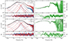 |
Fig. C.1. Best fit of the constant time-lag model applied to region Z3 of the HID of Cygnus X-1. Phase wrapping effects can be noticeable in the CS components, caused by the periodic zero-line crossing of the trigonometric functions. This effect is then propagated to the phase lags and the coherence function and becomes particularly noticeable at high frequencies. |
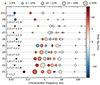 |
Fig. C.2. Covariance rms amplitude (%) and time lags (ms) of Cygnus X-1 derived from the τ-model applied to the 10 regions of the HID. The diamond marker is used to trace the QPO that coincides with the coherence drop. See Fig. 4 for details. |
NICER dataset properties up to Cycle 6 used in this work.
Phase-lag model summary.
Time-lag model summary.
All Tables
All Figures
|
Fig. 1. Hardness-intensity diagram computed from the unabsorbed fluxes of the NICER dataset of Cygnus X-1. The hardness ratio in x axis is defined as the ratio of the unabsorbed flux in the 2 − 12 keV band to that in 0.3 − 2 keV band, while the y axis is the unabsorbed flux in the 0.3 − 12 keV band. The fluxes were obtained from the fitting each 128 s segment with a model consisting of disc black body plus a power-law component, both affected by interstellar absorption. The different colours indicate the 10 distinct regions we use in this paper, parametrized by the increasing spectral index, Γ, of the power-law component (see legend). The grey error bars in the main panel indicate the 1σ errors of the fluxes and hardness ratios. Top-right inset panel: HID of Cygnus X-1 computed from the observed count rates in the same energy bands as in the main panel; the black points correspond to the segments we used in this work, whereas the grey points are the segments that we discarded in our analysis (see text for details). |
| In the text | |
|
Fig. 2. Phase lags in radians (colour points) and intrinsic coherence (gray points) of each region of the HID of Cygnus X-1 restricted to frequencies between 0.02 Hz and 30 Hz. The vertical stripe indicates the minimum of the coherence drop and the maximum of the cliff of the phase lags. The phase lags and coherence are computed between 0.3−2 keV and 2−12 keV energy bands, with the latter used as a reference band. |
| In the text | |
|
Fig. 3. Phase lags and intrinsic coherence function of region Z3 of the HID of Cygnus X-1 computed between the 3−5 keV and 5−12 keV energy bands. No evidence of the coherence drop or the cliff of the phase lags at ∼1.5 Hz is apparent (see Fig. 2). The horizontal lines in each panel indicate the reference levels for zero phase lag and unity coherence, respectively. |
| In the text | |
|
Fig. 4. Bubble plot of every Lorentzian in each HID region (vertical axis) of Cygnus X-1 as a function of their characteristic frequency (horizontal axis). The area of each bubble is proportional to the covariance rms amplitude of the Lorentzian. The colour scheme indicates the corresponding phase lag. The diamond marker highlights the narrow QPO responsible for the sharp coherence drop, which becomes apparent in Zones 3 to 8, corresponding to intermediate states with 1.8 < Γ < 2.4. |
| In the text | |
|
Fig. 5. Constant phase-lag model applied to region Z3 of the HID of Cygnus X-1. The top-left panels show the soft (0.3 − 2 keV) and hard (2 − 12 keV) PDS in rms2 units and residuals. The bottom-left panels show the real and imaginary parts of the cross spectrum (with the cross vector rotated by π/4) in rms2 units and the residuals. The top-right panels show the phase lags (rad) with the derived model and residuals. The bottom-right panels show the intrinsic coherence with the derived model and residuals. As described in the text, the model lines drawn in the right panels have not been fitted to the phase lags and the coherence but have been derived from the fits to the PDS and CS in the left panels. The QPO responsible for the coherence drop is highlighted over the other Lorentzians using a thicker line (at ν ∼ 1.3 Hz). The solid lines in the plots of the phase lags and coherence function show the derived model of those two quantities for ten Lorentzians (see text). Because the total phase lag spectrum and coherence function are not a combination of additive components, in these plots we cannot show the contribution of each Lorentzian. To show the effect of the imaginary QPO, the dashed lines in the plots show the derived models without the Lorentzian associated with the Imaginary QPO (without refitting the data). |
| In the text | |
|
Fig. 6. Covariance rms amplitude (in percent, left column) and phase lags (radians, right panel) of the imaginary QPO that cause the coherence drop of Cygnus X-1 as a function of energy. The centroid frequency of the imaginary QPO is indicated in each panel. A cubic polynomial has been fitted in each case to track the corresponding minima or maxima. In each panel, we show cubic model realisations in grey that depict the 1σ confidence range of the fits. |
| In the text | |
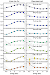 |
Fig. 7. Same as Fig. 6 but for the high-frequency bump in Cygnus X-1. |
| In the text | |
|
Fig. 8. Characteristic frequency of the high-frequency bump of Cygnus X-1 as a function of a linear combination of the spectral index, Γ, and the frequency of the imaginary QPO, νQPO. Top insets show the individual correlations. The best-fit linear model is shown in red. |
| In the text | |
|
Fig. C.1. Best fit of the constant time-lag model applied to region Z3 of the HID of Cygnus X-1. Phase wrapping effects can be noticeable in the CS components, caused by the periodic zero-line crossing of the trigonometric functions. This effect is then propagated to the phase lags and the coherence function and becomes particularly noticeable at high frequencies. |
| In the text | |
|
Fig. C.2. Covariance rms amplitude (%) and time lags (ms) of Cygnus X-1 derived from the τ-model applied to the 10 regions of the HID. The diamond marker is used to trace the QPO that coincides with the coherence drop. See Fig. 4 for details. |
| In the text | |
Current usage metrics show cumulative count of Article Views (full-text article views including HTML views, PDF and ePub downloads, according to the available data) and Abstracts Views on Vision4Press platform.
Data correspond to usage on the plateform after 2015. The current usage metrics is available 48-96 hours after online publication and is updated daily on week days.
Initial download of the metrics may take a while.