| Issue |
A&A
Volume 697, May 2025
|
|
|---|---|---|
| Article Number | A229 | |
| Number of page(s) | 17 | |
| Section | Astrophysical processes | |
| DOI | https://doi.org/10.1051/0004-6361/202453538 | |
| Published online | 23 May 2025 | |
Evolution of the Comptonizing medium of the black-hole candidate Swift J1727.8–1613 along the hard to hard-intermediate state transition using NICER
1
Observatoire Astronomique de Strasbourg, Université de Strasbourg, CNRS, 11 rue de l’Université, F-67000 Strasbourg, France
2
Kapteyn Astronomical Institute, University of Groningen, PO BOX 800, Groningen NL-9700 AV, The Netherlands
3
Instituto Argentino de Radioastronomí (CCT La Plata, CONICET; CICPBA; UNLP), C.C.5, (1894) Villa Elisa, Buenos Aires, Argentina
⋆ Corresponding authors: This email address is being protected from spambots. You need JavaScript enabled to view it.
, This email address is being protected from spambots. You need JavaScript enabled to view it.
Received:
20
December
2024
Accepted:
5
April
2025
Abstract
We analyse the properties of the Comptonizing medium in the black-hole X-ray binary Swift J1727.8−1613 using the time-dependent Comptonization model vkompth, applied to NICER observations of type-C QPOs in the hard and hard-intermediate states. During the 2023 outburst of the source, we measure the RMS and phase lags of the QPO across 45 observations as the QPO frequency, νQPO, evolves from ∼0.3 Hz to ∼7 Hz. By simultaneously fitting the time-averaged spectrum of the source and the RMS and lag spectra of the QPO, we derive the evolution of the disc and corona parameters. At νQPO = 0.34 Hz, the QPO phase lags are hard, with 10 keV photons lagging 0.5 keV photons by ∼0.5 rad. As νQPO increases, the lags for the same energy bands decrease, reaching near zero at νQPO∼1.2 Hz, and then reverse to soft lags of ∼−1.1 rad at νQPO∼7 Hz. Initially, the inner radius of the accretion disc is truncated at ∼30−40Rg (assuming a 10 solar-mass black hole) and, as the QPO frequency increases, the truncation radius decreases down to ∼10Rg. Initially, two coronas of sizes of ∼6.5×10³ km and ∼2×10³ km, extend over the disc and are illuminated by different regions of the disk. As the QPO frequency increases, both the coronas shrink to ∼2×10³ km at νQPO = 2.5 Hz. Following a data gap, one corona expands again, peaking at a size of ∼2×10⁴ km. We interpret the evolution of the coronal size in the context of accompanying radio observations, discussing its implications for the interplay between the corona and the jet.
Key words: accretion, accretion disks / black hole physics / methods: data analysis / stars: black holes / X-rays: binaries / X-rays: individuals: Swift J1727.8–1613
© The Authors 2025
 Open Access article, published by EDP Sciences, under the terms of the Creative Commons Attribution License (https://creativecommons.org/licenses/by/4.0), which permits unrestricted use, distribution, and reproduction in any medium, provided the original work is properly cited.
This article is published in open access under the Subscribe to Open model. This email address is being protected from spambots. You need JavaScript enabled to view it. to support open access publication.
1. Introduction
Transient black hole X-ray binary (BHXB) systems generally remain in a quiescent state, exhibiting low X-ray flux levels. Before entering into outburst, they often show optical variability, which is seen as a precursor to the impending outburst (e.g., Hameury et al. 1997). During the outburst phase, these systems undergo notable X-ray flux variability across various energy bands (see, e.g., Remillard & McClintock 2006; Motta et al. 2012). The X-ray spectrum of these sources typically features a disc black-body component that dominates the low energies (Shakura & Sunyaev 1973), along with a power-law component that can extend up to ∼1 MeV (Cadolle Bel et al. 2006). This non-thermal component is believed to result from the inverse Comptonization of seed-photons from the accretion disc (e.g. Gierlinski et al. 1997). Moreover, the spectra of these sources often include an iron emission line in the 6–7 keV range, the profile of which is used to probe the black-hole spin (e.g. Reynolds & Fabian 2008). Additionally, a Compton reflection hump is commonly observed around 20–30 keV (Basko et al. 1974; Magdziarz & Zdziarski 1995). Since these spectral components dominate distinct energy ranges, variability in flux or photon counts across these bands is frequently analysed to interpret changes in the system's accretion state.
Timing studies of various BHXBs have shown that these systems exhibit a hysteresis loop in the hardness-intensity diagram (HID) during outbursts (e.g. Homan et al. 2001). The accretion states are classified based on the source's position within the HID. In this context, the low-hard state (LHS) is identified by a high hardness ratio and low flux, while the high-soft state (HSS) features high flux and a low hardness ratio (Belloni et al. 2005, 2011; Done et al. 2007, and references therein). Additionally, two intermediate states in between these two extreme states are recognised as the hard intermediate state (HIMS) and the soft intermediate state (SIMS). In the HSS the X-ray spectrum is dominated by blackbody disc emission, whereas the non-thermal component prevails in the LHS. The LHS spectrum is characterised by a power law with a photon index of approximately 1.5–2.0 (Gilfanov 2010), while the HSS includes a softer power-law component with a photon index of Γ≥2.5 (Méndez & van der Klis 1997; Remillard & McClintock 2006; Done et al. 2007).
Black hole X-ray binaries exhibit variability in their X-ray light curves, which we analyse in the Fourier domain using power density spectra (PDS, see van der Klis & Jansen 1985). The PDS reveal significant variability in BHXB across a wide range of timescales; the most important variability components are the quasi-periodic oscillations (QPOs, see Chen et al. 1997; Takizawa et al. 1997; Psaltis et al. 1999; Nowak 2000), categorised into mHz QPOs, low-frequency QPOs (LFQPOs), and High-Frequency QPOs (for a review, see Ingram & Motta 2019, and references therein). LFQPOs occurring between 0.1 and 30 Hz, are further classified as Type-A, Type-B, and Type-C (Wijnands et al. 1999; Homan et al. 2001; Remillard et al. 2002; Casella et al. 2004). Type-C QPOs are the most frequently observed, typically appearing in the LHS and HIMS (see Motta et al. 2015, and references therein). In the PDS, these QPOs feature a large fractional root mean square (RMS) amplitude, often accompanied by a harmonic component at twice the QPO frequency, along with a broad Lorentzian noise component and occasionally a sub-harmonic component (Belloni et al. 2002; Casella et al. 2004). Transient BXBs trace an oval-shaped wheel in the power colour-colour diagram, where the angle along the wheel (the hue) can be used to identify the canonical accretion states of these systems (see Heil et al. 2015, for details).
Despite their prevalence in BHXB, the origin of these QPOs remains a subject of debate within the X-ray astronomy community, particularly between two prevailing models. One class of model considers that the LFQPOs are due to a geometric mechanism, as described by the relativistic precession model (RPM; Stella & Vietri 1998; Stella et al. 1999), where the type-C QPO frequency would correspond to the Lense-Thirring precession frequency around the black hole (Lense & Thirring 1918). The RPM has been tested in BHXB systems such as GRO J1655–40 (Motta et al. 2014a), XTE J1550-564 (Motta et al. 2014b), and MAXI J1820+070 (Bhargava et al. 2021, and references therein). An alternative class of models suggests a dynamical rather than a geometric mechanism for LFQPOs, including accretion-ejection instabilities in a magnetised disc (Tagger & Pellat 1999), oscillations in a transition layer within the accretion flow (Titarchuk & Fiorito 2004), and corona oscillations driven by magnetoacoustic waves (Cabanac et al. 2010; O’Neill et al. 2011). In this context, LFQPOs have been associated with the relativistic dynamic frequency of a truncated accretion disc in BHXB such as GRS 1915+105 (Misra et al. 2020; Liu et al. 2021), MAXI J1535–571 and H1743–322 (Rawat et al. 2023a), GX 339–4, and EXO 1846–031 (Zhang et al. 2024).
The timing and spectral properties of X-ray binaries have been widely used to investigate the physical and geometric characteristics of disk-corona systems, specifically through phase lags and RMS amplitude spectra at QPO frequencies (Lee & Miller 1998; Lee et al. 2001; Kumar & Misra 2014). This approach assumes that the flux oscillations in the time-averaged spectrum – modulated at the QPO frequency – are driven by oscillations in the thermodynamic properties of the Comptonizing region. These properties include the temperature and external heating rate of the corona, the electron density within the corona, and the temperature of the soft photon source, which provides seed-photons for Comptonization. Karpouzas et al. (2020) introduced vkompth, an improved model building on the earlier model by Kumar & Misra (2014) with enhanced equation-solving techniques. Originally designed for neutron star binaries, this model was later adapted for black-hole binaries as well (Bellavita et al. 2022). While this model describes the radiative properties of the QPO (RMS amplitude and lags) in terms of feedback loop between the corona and the disk, the same feedback mechanism can explain the QPO frequency (Mastichiadis et al. 2022). To date, the model has effectively explained comptonizing medium properties through type-A, type-B, and/or type-C QPOs in BHXB systems, including GRS 1915+105 (Méndez et al. 2022; García et al. 2022), MAXI J1535–571 (Zhang et al. 2022, 2023a; Rawat et al. 2023b), GRO J1655-40 (Rout et al. 2023), MAXI J1820+070 (Ma et al. 2023), and MAXI J1348−630 (García et al. 2021; Zhang et al. 2023b; Alabarta et al. 2025).
Swift J1727.8–1613 (Swift J1727 hereafter) is a BHXB source first detected on August 24 2023 with Swift/BAT (Page et al. 2023) and initially classified as a GRB source but later identified as a BHXB source with MAXI/GSC (Negoro et al. 2023) and NICER (O’Connor et al. 2023). Using the GTC-10.4m telescope, Mata Sánchez et al. (2024) proposed that the companion star is an early K-type star and estimated an orbital period of ∼7.6 h and a distance to the source of 2.7 ± 0.3 kpc. With the Very Long Baseline Array and the Long Baseline Array, Wood et al. (2024) imaged Swift J1727 during the hard/hard-intermediate state, revealing a bright core and a large, two-sided, asymmetrical, resolved jet. The polarization properties of Swift J1727 indicate that the source has an inclination angle between 30−60° (Veledina et al. 2023).
During the initial phase of the outburst, observations with INTEGRAL, ART-XC, Swift/XRT, and AstroSat revealed a variable QPO in Swift J1727, with frequencies ranging from 0.8 Hz to 10.0 Hz (Mereminskiy et al. 2024; Nandi et al. 2024). With IXPE, a QPO with a frequency evolving from approximately 1.3 Hz to 8.0 Hz was also reported in the 2–8 keV energy band by Ingram et al. (2024). Observations with IXPE and NICER from August to September 2023 showed that the source transitioned from the LHS to the HIMS, accompanied by a significant decrease in the polarization fraction from about 4% to 3% (Ingram et al. 2024). Using INTEGRAL/IBIS, Bouchet et al. (2024) reported a highly polarised spectral component above 210 keV, present in both the HIMS and the initial phases of the SIMS. Interestingly, during the HIMS, the polarization angle (PA) differs from the angle of the compact jet projected onto the sky, while in the SIMS the two angles are closely aligned (Bouchet et al. 2024). During the decay of the outburst, back in the LHS (during February 2024), the PA remained constant at the same value as at the one during the rising part, while the polarization fraction increased with X-ray hardness (4–8 keV/2–4 keV; Podgorný et al. 2024).
In this work, we analyse NICER observations of Swift J1727 during its LHS and HIMS to study the Comptonizing medium properties through the type-C QPOs using the vkompth model. In Section 2 we provide details of the observations, instrument specifications, and the spectral and timing analysis techniques applied. The fits to the RMS, lag and time-averaged spectra at the type-C QPO are presented in Section 3. We discuss the implications of these findings and interpret them within the disk-corona framework in Section 4.
2. Observations and data analysis
The Neutron Star Interior Composition Explorer (NICER), launched on June 2, 2017, is mounted on the International Space Station (Gendreau et al. 2016). Its X-ray Timing Instrument operates within the 0.2–12.0 keV energy range, with an effective area exceeding 2000 cm2 at 1.5 keV. NICER provides an energy resolution of 85 eV at 1 keV and a time resolution of 4 × 10⁻⁸ s. We used NICER observations of Swift J1727 from 2023-08-26 to 2023-10-09, with observation details presented in Table A.1.
We processed each observation using the nicerl2 task, applying standard calibration and screening procedures. By default, nicerl2 uses the ‘night’ threshold setting, but there are observations with no exposure during the night; for those observations, we set threshfilter=DAY. We used either day or night data for an individual observation, because NICER has been affected by optical light leakage on May 2023 and hence separate analysis of orbit day and orbit night data is recommended by the NICER team1. We only used observations where the exposure time is greater than 200 seconds after running the nicerl2 task. Next, we extracted light curves in the 0.3–4.0 keV, 8.0–12.0 keV, and 0.5–10.0 keV energy bands using the nicerl3-lc task. The left panel of Figure 1 shows the MAXI light curve for Swift J1727, with NICER observations highlighted in the shaded grey regions. Details of the NICER count rates are provided in Appendix Table A.1. We then calculated the hardness ratio as the number of photons in the 5.0–10.0 keV band divided by those in the 0.5–2.0 keV band. We segment the observations where a significant change in both the full-band count rate and hardness ratio was observed. To illustrate the source evolution, we plot the HID using NICER data in the Figure 2. The colour scale on the right side of that Figure represents time, with red corresponding to MJD 60181 and transitioning to navy blue at MJD 60226, 45 days later.
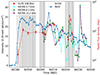 |
Fig. 1. MAXI light curve of Swift J1727.8–1613 starting from 60175 MJD (August 19, 2023) in the 2–20 keV energy band in units of photons s−1 cm−2 (blue triangles; left y axis). The right y-axis shows the radio flux density in mJy from the VLA Low-band Ionosphere and Transient Experiment (VLITE) at 338 MHz (red data points, data from Peters et al. 2023), alongside RATAN-600 observations at frequencies of 4.7 GHz (cyan data points), 8.2 GHz (green data points), and 11.2 GHz (purple data points, data from Ingram et al. 2024). |
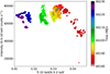 |
Fig. 2. NICER hardness-intensity diagram starting from MJD 60181. The intensity is the 0.5–10.0 keV count rate and the hardness is the ratio of the count rate in the 5–10 keV band to that in the 0.5–2.0 keV band, with data points binned over 100 seconds. The colour scale indicates the MJD. |
2.1. Timing analysis
We extracted the fractional RMS normalised (Belloni & Hasinger 1990) PDS and cross spectrum for each observation using the General High-energy Aperiodic Timing Software (GHATS)2 V3.1.0. We used the novel technique proposed by Méndez et al. (2024) to measure the phase lags. For each observation, we first extracted the 0.5–10.0 keV PDS and the cross spectrum between the 0.5–2.0 keV and 2.0–10.0 keV energy bands. We fit the PDS with a combination of Lorentzian functions together with the real and imaginary parts of the cross spectrum. For each component present in the PDS, we fit the real and imaginary part of the cross spectrum with Lorentzians multiplied by cos(Δϕ) and sin(Δϕ), respectively with the centroid and width of each Lorentzian tied to the parameters in the PDS, where Δϕ is the phase lag.
We observe that the QPO centroid frequency varies from 0.3 Hz to 7.0 Hz (Appendix Table A.1). For some observations marked with a * in Appendix Table A.1, the QPO detection was below 3 sigma, so these observations were excluded from further analysis. Additionally, for obs no. 3 and 4, the QPO was weak in the 0.5–10.0 keV band, and therefore, these observations were also excluded from further study. To measure the phase-lag and RMS spectra, we divide the energy bands into 38 bins, starting from 0.5 keV to 7.9 keV with a bin size of 0.2 keV, and a last bin that spans from 7.9 keV to 10 keV due to the QPO being weaker in the highest energy band. For some observations (mainly those where we segmented the observation into parts or the QPO frequency exceeded 2.5 Hz), the QPO fractional RMS was low (as shown in Appendix Table A.1), making the QPO insignificant with finer binning. To address this in those observations, we manually merge the bins in regions where the signal was weak, resulting in 11 energy bands: 0.5–0.9 keV, 0.9–1.3 keV, 1.3–1.7 keV, 1.7–2.1 keV, 2.1–2.9 keV, 2.9–3.7 keV, 3.7–4.5 keV, 4.5–5.7 keV, 5.7–6.5 keV, 6.5–7.7 keV, and 7.7–10.0 keV. For each band we extract the phase lag and RMS using the technique of Méndez et al. (2024) discussed above using the 0.5–10.0 keV band as the reference. To account for the correlation due to photons being present in both the subject and reference bands, we include a constant term in the model of the real part of the cross-spectrum.
2.2. Spectral analysis
We used the nicerl3-spect task to extract source and background spectra, response (rmf) and ancillary response (arf) files in the 0.5–10.0 keV band. We used Heasoft version 6.33 and CALDB version 20240206. We fitted the background-subtracted time-averaged spectrum of the source using the model TBfeo*(diskbb + gaussian + nthComp) in Xspec 12.14.0. The TBfeo model is similar to the tbabs model, which accounts for interstellar absorption, but allows the oxygen and iron abundances to vary, in addition to the hydrogen column density. We used the cross-section tables of Verner et al. (1996) and the abundances of Wilms et al. (2000) and left the hydrogen column density as a free parameter. We have frozen the oxygen and iron abundance relative to Solar to 1 and the redshift to zero. The diskbb component models the thermal emission from an optically thick and geometrically thin accretion disc (Mitsuda et al. 1984; Makishima et al. 1986) while nthcomp (Zdziarski et al. 1996; Życki et al. 1999) models the Comptonised emission from the X-ray corona. We kept both diskbb parameters, the temperature at the inner disc radius, kTin, and the normalisation free. The nthcomp model parameters are the power-law photon index, Γ, electron temperature, kTe, seed-photon temperature, kTbb, and normalisation. The seed-photon temperature kTbb was tied to kTin of the diskbb component. Since the electron temperature of nthcomp could not be constrained with the NICER data, following Bouchet et al. (2024) we fixed it at 40 keV for observations 2 to 36 and at 250 keV for observations 37 to 54. We modelled the relatively broad iron line present in the residuals of observations 1 to 17 with a Gaussian fixed at 6.4 keV using the gauss model.
2.3. Time-dependent Comptonization model
To study the properties of the Comptonizing medium, we model the RMS and phase-lag spectra of the QPO with the time-dependent Comptonization model vkompth3. The time-averaged variant of vkompth model is identical to the thermal Comptonization model nthComp, but vkompth incorporates additional parameters that only impact the time-dependent version of the model. In the case of a disk-blackbody soft photon-source, the vkompth model has two versions: one for a single corona, vkompthdk, and second for a dual corona, vkdualdk. The model parameters for vkompthdk are the seed-photon temperature, kTs, the electron temperature, kTe, the photon index, Γ, the corona size, L, the feedback fraction, η, the size of the seed-photon source, af, the amplitude of the variability of the external heating rate,  , and the reference lag of the model in the 0.5–10.0 keV energy band, reflag. Since the vkompth model is not sensitive to af, we fix this parameter at 250 km (for details, see García et al. 2022). The parameter reflag is an additive normalisation that allows the model to match the data, given that the observer is free to choose the reference energy band of the lags. The vkdualdk model (García et al. 2021; Bellavita et al. 2022) has two sets of coronal parameters, kTs, 1/kTs, 2, kTe, 1/kTe, 2, Γ1/Γ2, L1/L2, η1/η2, and
  to describe the physical properties of the two coronal regions. The remaining parameters of the dual models are the size of the seed-photon source and the reference lag, plus an additional parameter, ϕ, which describes the phase difference between the two coupled coronae (for more details see García et al. 2021). To model the RMS spectra of the QPO, we incorporate a multiplicative dilution component, which is a function of energy (E). This component accounts for the fact that the RMS amplitude we observe is diluted by the emission of the other components that we assume do not vary (see details in Bellavita et al. 2022). We linked the parameters of the dilution component to the corresponding parameter of the model of the time-averaged spectrum. We will discuss the results of the fit in detail in Section 3.2.
3. Results
We present the MAXI light curve of Swift J1727 during its outburst in August 2023 in Figure 1. To show the simultaneous evolution of the source in radio, we over-plot the radio light curves obtained from the VLA Low-band Ionosphere and Transient Experiment (VLITE) 338 MHz (data from Peters et al. 2023), along with the RATAN-600 observations at 4.7 GHz, 8.2 GHz and 11.2 GHz (data from Ingram et al. 2024). The MAXI flux in the 2–20 keV band rises from ∼0.5 photons s−1 cm−2 to ∼25 photons s−1 cm−2 over a period of 5 days, starting from MJD 60180 (August 24, 2023). The VLITE light curve shows a significant increase in radio flux starting from MJD 60181.98 that remains more or less constant until MJD 60204.04. The X-ray flux then decreases to ∼5 photons s−1 cm−2 over nearly two months, with several X-ray and radio flares occurring in between. The VLITE data show two radio flares on MJD 60209.99 and MJD 60223.04, while a very bright radio flare is visible in the RATAN-600 data at 4.7 GHz, 8.2 GHz, 11.2 GHz frequencies on MJD 60231.54. We mark the times of the NICER observations with grey regions in Figure 1. The NICER 0.5−10.0 keV count rate initially increases from ∼1.5 ×10⁴ counts s−1 to ∼7.5 ×10⁴ counts s−1. Simultaneously, the HR of the source decreases from ∼0.045 to ∼0.035, indicating a clear evolution from the LHS to the HIMS as shown in Figure 2. The HR decreases further from approximately ∼0.035 to ∼0.015, while the flux continues to decrease monotonically, reaching around ∼5.7 ×10⁴ counts s−1.
3.1. Timing results
Adopting the method of Belloni et al. (2002), we fit the PDS with four to five Lorentzian components. Following Méndez et al. (2024), we used the same combination of Lorentzians to fit the real and imaginary parts of the cross spectra multiplied by, respectively, the cosine and sine of the phase lags which, for each individual Lorentzian, are assumed to be constant with frequency. During the fits we link the frequencies and full width at half maximum of each Lorentzian in the PDS and cross spectra. The model includes two components that represent the broadband noise: (1) a zero-centred Lorentzian representing the low frequency broad-band noise and (2) a high-frequency broad noise component around 11.0 Hz. To fit the narrow peak components, which we identify as the QPO and its second harmonic, we used two separate Lorentzians. While fitting the harmonic component, we set the Lorentzian centroid frequency and width to twice the corresponding values of the QPO fundamental. For QPO centroid frequencies of less than 3.0 Hz, the PDS also shows a low-frequency noise component (see, for example, the top left panel of Figure 3). We include an additional Lorentzian to account for this feature whenever required.
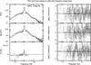 |
Fig. 3. Top left panel displays the 0.5–10.0 keV power density spectrum of Swift J1727.8–1613, fitted with five Lorentzians for ObsID 6203980105. The middle and bottom left panels show the real and imaginary parts of the cross spectrum between the 0.5–2.0 keV and 2.0–10.0 keV bands, along with the best-fitting model that assumes that the phase lags of each Lorentzians are constant with Fourier frequency (see Méndez et al. 2024). The right-hand panels display the residuals of the fits for the respective spectra. |
We show the fit to the PDS and the real and imaginary part of the cross spectrum of OBSID 6203980105 in Figure 3. The top left panel shows the PDS and the right panel shows the residuals of the fit. The PDS shows a significant narrow QPO component at ∼0.89 Hz with a harmonic component at twice that frequency. On the basis of strength of the QPO and the presence of a harmonic, and broad noise components, we identify this as a type-C QPO. In the middle left and bottom left panels of Figure 3, we display the real and imaginary parts of the cross spectrum, along with the corresponding residuals of the fit in the middle and bottom-right panels. For ObsID 6557020402, which features a QPO at approximately 7.0 Hz, we present the PDS and the real and imaginary parts of the cross spectrum in Appendix Figure A.1. The real part of the cross spectrum contains the same number of Lorentzians as the PDS. Meanwhile, the imaginary part shifts from positive to negative as the QPO frequency increases from 0.3 to 7.0 Hz (see bottom left panel of Figure 3 and Appendix Figure A.1).
The QPO frequency increases monotonically from 0.3 Hz to 1.4 Hz over time until MJD 60196, as shown in Figure 4 (see also Appendix Table A.1). Between MJD 60199 and MJD 60201, the QPO frequency abruptly increases from 2.3 Hz to 3.3 Hz, then drops to 2.0 Hz within a span of just one day. The QPO frequency then increases further to 7.0 Hz, with a gap in NICER data between MJD 60203 and MJD 60219. The colour scale on the right side of the Figure indicates the QPO fractional RMS in the 0.5−10.0 keV band. The QPO fractional RMS first increases from 7.6% to 9.3% as the QPO frequency increases from ∼0.3 Hz to ∼0.8 Hz, and then decreases from 9.3% to ∼1% as the QPO frequency increases from ∼1 Hz to ∼7 Hz at the end of the NICER observations (see also Appendix Table A.1). During the period, where the QPO frequency exhibits an abrupt increase and then decreases, the fractional RMS remains anti correlated. This behaviour of the fractional RMS is similar to that observed in other BHXB sources like GRS 1915+105 (Zhang et al. 2020), and MAXI J1535−571 (Rawat et al. 2023b). We give details of the QPO centroid frequency, width and fractional RMS in the 0.5–10.0 keV band in Appendix Table A.1.
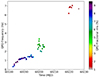 |
Fig. 4. QPO frequency of Swift J1727.8–1613 as a function of MJD. The colour bar gives the QPO fractional RMS amplitude in the 0.5–10.0 keV energy range. |
We show the QPO phase lag spectra at five QPO frequencies, 0.34 Hz, 0.79 Hz, 1.22 Hz, 2.56 Hz, 6.19 Hz, and 7.02 Hz, in Figure 5. At a QPO frequency of 0.34 Hz, the phase lags are negative at low energies and become positive at ∼1.5 keV, continue increasing and become more or less constant at 0.25 rad above ∼3 keV. The lags increase with energy when νQPO≤0.34 Hz, flatten for 0.79 Hz < νQPO≤ 2.56 Hz, and decrease with energy when νQPO≥6.19 Hz. Additionally, the lags show minima that shift to higher energies as a function of QPO frequency. At νQPO = 0.34 Hz, the minimum appears between 0.5 and 1.0 keV; for 0.79 Hz < νQPO≤2.56 Hz, the minimum shifts to 1.5–2.0 keV, and by νQPO≥6.19 Hz, the minimum is at around 4 keV. A similar shift in the phase-lag spectra minima is also observed for the type-B QPOs in MAXI J1348–630 and for the type-C QPOs in MAXI J1535–571 (Rawat et al. 2023b). We also computed the time lag of the 2.0–10.0 keV band with respect to 0.5–2.0 keV band, across all observations (see the second row of Appendix Tables A.2, A.3, A.4 and A.5).
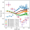 |
Fig. 5. Phase-lag spectra corresponding to specific QPO frequencies, from 0.34 Hz to 7.02 Hz. The reference energy band used here for the lags is 0.5–10.0 keV. |
3.2. Spectral-timing results
We fit simultaneously the RMS spectrum of the QPO with the model vkompthdk*dilution, the phase-lag spectrum of the QPO with the model vkompthdk and the time averaged spectrum of the source with model described in Section 2.2. We tie kTe and Γ of vkompthdk to kTe and Γ of nthcomp, and link all other parameters of vkompthdk between the lag spectra and the RMS spectra. While fitting the vkompthdk model, we initially tied the diskbb temperature (kTin) to the seed photon temperature (kTs) of vkompthdk. However, the model was unable to reproduce the valley in the phase lag spectrum and gives a χ2/d.o.f. of 1748.1/253. A similar behaviour was observed in the black hole X-ray binary MAXI J1535–571 when modelled with vkompthdk, where the fit improves significantly when kTin and kTs were untied (see Figure 6 of Rawat et al. 2023b). To address this, we allowed kTin and kTs to vary independently, and found two separate sources of seed photon; one with a temperature of kTin∼0.35 keV, responsible for producing the steady-state spectra, and another with a temperature of kTs∼0.06 keV, which contributes to the phase lag and RMS spectra. As an example, we show the time averaged spectrum of the source fitted with the model TBfeo*(diskbb + gaussian + nthComp), and the RMS and phase-lag spectra of the QPO at 0.89 Hz fitted with the model vkompthdk*dilution and vkompthdk in, respectively, the top, middle and bottom panels of Figure 6, with the vkompthdk model plotted in blue in the middle and bottom panels (obs no. 6). As it appears from the Figure, vkompthdk still cannot fit the minimum of the phase-lag spectra properly, yielding a chi-square of 415.2 for dof 255 (see Table 1 for best fit parameters).
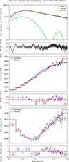 |
Fig. 6. Top panel shows the NICER time-averaged spectrum of Swift J1727.8–1613 (ObsID 6203980105) with a QPO centroid frequency of 0.89 Hz, fitted using the model TBfeo*(diskbb + gaussian + nthComp) together with the residuals of the best-fitting model. The middle panel shows the RMS spectrum of the QPO fitted with the vkdualdk*dilution (red) and vkompthdk*dilution (blue) models with the residuals of the best-fitting model. The bottom panel shows the phase-lag spectrum of at the QPO fitted with the vkdualdk (red) and vkompthdk model (blue) with the residuals of the best-fitting model. The 0.5–10.0 keV energy band is used as the reference for the phase-lag spectra. |
Representative best-fitting spectral and corona parameters for ObsID 6203980105 of Swift J1727.8–1613 using the single and dual corona model.
Next we fit the RMS spectra of the QPO with the model vkdualdk*dilution (Karpouzas et al. 2020; Bellavita et al. 2022) and the lag spectra of the QPO with the model vkdualdk. We tie kTe, 1/kTe, 2 of vkompthdk to kTe of nthcomp, Γ1/Γ2 of vkompthdk to Γ of nthcomp, and link all the parameters of vkompthdk between the lag spectra and the RMS spectra. We allowed the seed photon temperature of the first corona, kTs, 1, to vary independently, while tying the seed photon temperature of the second corona, kTs, 2, to the inner disc temperature, kTin. The chi-square for the fit with a dual-corona model decreases to 254.2 for dof 251 (obs no. 6). We give the best-fitting parameters for obs no. 6 in Table 1 along with the chi-square of the fits for both models. In the middle and bottom panels of Figure 6, the solid red line represents the best fit model of vkdualdk*dilution and vkdualdk to, respectively, the RMS and phase-lag spectra of the QPO. The corner plot of the spectral parameters for obs no. 6, generated using pyXspecCorner4, is shown in Figure A.3. During the period MJD 60181–60199, the phase-lag spectra at the QPO frequency are flat (1.0 Hz < νQPO <2.5 Hz). The phase lag spectra are reasonably well-fitted by the single-corona model vkompthdk; however, when a valley is evident in the lag spectra (see Figure 5), fits using the dual-corona model, vkdualdk, provide statistically better results.
For most observation in the period MJD 60199–60203 (obs. 28–42), the dual-corona model appears to over-fit the data, while the single-corona model provides statistically acceptable fits. For instance, in observation 32, the single-corona model yields χ2/d.o.f. = 115.7/153. In these cases, the over-fitting of the dual-corona model may be explained by the decreasing QPO RMS amplitude over time or, in some cases, by shorter exposure times, which result in the RMS and lag spectra being less able to constrain the model parameters. Nevertheless, even in cases where the dual-corona model over-fit the data, the sizes of the two coronas remain consistent with each other, similar to the earlier period. For the few observations in this period where the dual-corona model still provides a statistically better fit (see Tables A.2–A.5), the sizes of the two coronas again remain in good agreement. To avoid inconsistencies in our analysis by switching between single and dual-corona models, we opt to fit all observations in with the dual-corona model. In cases where the dual-corona model over-fits the data, we link the sizes of the two coronas to be the same, ensuring a coherent and systematic approach to the modelling.
After the data gap between observations 42 (MJD 60203.4) and 43 (MJD 60219.7), the size of the second corona can no longer be constrained when fitting with the dual-corona model. We initially tied the parameters of the two coronas, but since the lag is not flat in these observations, unlike in previous ones, the single-corona model could not produce the valley in the lag spectrum. First, we tied the sizes of both coronas (L1 and L2), which resulted in a reduced chi-square of 143.0/174 as shown in Figure A.2 (solid blue line). While this is statistically a good fit, the model still did not reproduce the observed phase lag valley. Next, we let the two corona sizes vary separately, but we were unable to constrain L2, likely due to the limited number of bins in those observations. We then fixed L2 to the value obtained in observation 39, the last one where the second corona can be reliably measured (L2 = 1.9×10³ km). This gives a χ2/d.o.f. of 128.5/173 and the model fits the valley of the phase lag spectra as shown by the solid red line in Figure A.2.
From the fits to the time-averaged spectrum of the source and the RMS and phase lag spectra of the QPO, we find that during the hard and hard-intermediate states, the inner disc temperature, kTin, increases from ∼0.27 keV to ∼0.73 keV with time as shown in the left panel of Figure 7. The power-law index increases from ∼1.6 to ∼3.0, which highlights the evolution of the source from the hard to the hard-intermediate state during the course of the observations, as shown in the right panel of Figure 7. The coronal seed temperature, kTs, 1 also increases from ∼0.25 keV to ∼0.70 keV. We show the evolution of kTs, 1 in the top left panel of Figure 7. The kTin, kTs, 1 and power-law index increase and then decrease as a function of time between MJD 60199 and MJD 60201.
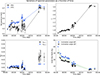 |
Fig. 7. Top left panel shows the inner disc temperature, kTin, and coronal seed temperature, kTs, 1, as a function of time for Swift J1727.8–1613. The top right panel presents the power-law photon index of NTHCOMP, Γ, as a function of time. The bottom left panel displays the time evolution of the intrinsic feedback fraction, ηint, 1 and ηint, 2, obtained from the fit with the vkdualdk model. The bottom right panel shows the evolution of the inner disc radius (in units of gravitational radii) for inclination angles of 60° (blue) and 30° (black). For the calculation of the inner disc radius, we used a spectral hardening factor Tcol/Teff of 1.7, assumed a M⊙ black hole, and set the distance to the source at 2.7 kpc. |
Using the parameters of vkdualdk we have computed the intrinsic feedback fraction, the fraction of the corona flux, ηint, 1 and ηint, 2, that returns to the disc (see Karpouzas et al. 2020 for details) from corona 1 (C1) and corona 2 (C2), respectively (given in Appendix Tables A.2–A.5). We show ηint, 1 and ηint, 2 as a function of time with the black and blue points in the bottom left panel of Figure 7, respectively. The intrinsic feedback fraction for both coronas is ∼2−5% when the QPO frequency is in the range 0.3–2.6 Hz. When the QPO frequency is above 2.6 Hz, the feedback fraction rises to ∼15−20% for corona 1 and to ∼10% for corona 2. We note that we have frozen the value of the feedback fraction in obs. 17, because it remained unconstrained otherwise.
Assuming that the source is at a distance of 2.7 kpc (Mata Sánchez et al. 2024) and has an inclination angle between 30−60° (Veledina et al. 2023), we translate the diskbb norm parameter (given in Appendix Tables A.2–A.5) to an inner disc radius, including a spectral hardening factor Tcol/Teff of 1.7 (Shimura & Takahara 1995; Kubota et al. 1998). Assuming that the system harbours a 10 M⊙ black hole, we compute the inner disc radii range in units of the gravitational radius, Rg=GM/c2, as shown in the bottom right panel of Figure 7 as a function of time. The shaded green region in Figure 7 shows that the inner disc radius decreases from 30–40 Rg to 5–7 Rg as the QPO frequency increases from 0.3 to 7.0 Hz.
The analysis reveals that, as the QPO frequency increases from 0.3 Hz to 2.5 Hz, L1 decreases from ∼6.5×10³ km to ∼2×10³ km with some fluctuations in between as shown in Figure 8. During the first observation, L2 starts at approximately ∼2×10³ km, expands to around ∼8×10³ km, and then contracts to nearly the same values as L1. For the first observation L2 is ∼2×10³ km, it then expands to ∼8×10³ km and then contracts to a size that is nearly equal to L1. This trend is also consistent with the results of Liao et al. (2024), which fit the vkompthdk model between MJDs 60198 to 60203 and find that the size of corona decreases from ∼2500 km to ∼1000 km and then increases again to ∼2000 km. After a gap of about two weeks in the data, the QPO is at frequency of ∼6 Hz. Assuming no further variation in the size of the second corona in the observations with QPO frequency in the 6–7 Hz range, which we fixed to 1.9×10³ km (see previous paragraph), the size of the first corona increases again, from ∼2×10³ km to ∼10×103 km at 6.0 Hz, and further to ∼15×103 km when the QPO frequency reaches 7.0 Hz. These findings are summarised in Tables A.2–A.5, where values fixed during the fitting process are indicated with square brackets. We provide all the parameters of both coronas for all the observations in Tables A.2–A.5.
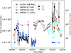 |
Fig. 8. Evolution of the sizes of the coronas, L1 and L2, for Swift J1727.8–1613 using the vkdualdk model. The right y axis shows the radio flux density in mJy obtained from the VLA Low-band Ionosphere and Transient Experiment (VLITE) at 338 MHz (red data points, data from Peters et al. 2023), alongside RATAN-600 observations at frequencies of 4.7 GHz (cyan data points), 8.2 GHz (green data points), and 11.2 GHz (purple data points, data from Ingram et al. 2024). |
4. Discussion
We analyse NICER observations of Swift J1727.8–1613 during the hard and hard-intermediate states of its first outburst, covering the period from MJD 60181 to 60226 (late August to mid-October 2023). The source shows type-C QPOs with centroid frequencies between 0.3 to 7.0 Hz. We model the time-averaged spectra of the source, as well as the RMS and phase-lag spectra of the QPO, using the time-dependent Comptonization model vkompth. At the start of the observations, approximately 90% of the total 2−20 keV flux comes from the corona and 5% comes from the disk, while by the end of the observations, the contribution of the corona and disc are 75% and 20%, respectively (see rows 6 and 10 of Table A.5). Our results indicate the presence of two horizontally extended coronas (C1 and C2 from now on) covering a truncated accretion disk. As the source progresses towards the HIMS, the inner disc moves closer to the black hole. Initially, C1 and C2 contract; later, C1 expands. The temperature of the seed-photon source for both coronae increases from 0.3 keV to 0.7 keV, suggesting the corona shifts inwards along with the disk. In an alternative scenario, the corona remains around 10 Rg from the black hole while the disc moves inwards, such that seed photons that illuminate come progressively from regions of the disc closer to the black hole. We discuss the evolution of the corona and other spectral parameters in the context of radio observations in Section 4.2.
The power-law index, Γ, reaches a value of ∼3 by the end of these observations. While Γ≥ 2.5 is typically associated with the soft-intermediate and soft states, the occurrence of Type-C QPOs, the slope of the power spectrum, the high amplitude of the broadband noise component, and the dominance of the non-thermal flux (comprising 80% of the total flux) indicate that in all these observations the source is in the hard-intermediate state. Furthermore, using the Power colour-colour diagram, and following the methodology outlined by Heil et al. (2015), Ingram et al. (2024) classified these observations as being in the hard-intermediate state, as shown in Figure 7 of their paper. Additionally, a photon index of Γ∼2.9 has been reported previously for the hard-intermediate state in the black hole binary GRS 1915+105 (Droulans & Jourdain 2009).
4.1. QPO lag spectrum: Evidence for a hard-to-soft lag transition
At lower QPO frequencies, νQPO∼0.3 Hz, the lag spectrum displays a hard lag, where the 2.0–10 keV photons lag behind the 0.5–2.0 keV band photons by approximately 0.3 rad, or 150 ms. For QPO frequencies in the range 0.8 Hz < νQPO≤1.2 Hz, the lag spectrum gradually flattens, with the lags fluctuating at around −0.1 rad and +0.1 rad. Here, the time lag between the 2.0–10 keV and 0.5–2.0 keV bands decreases progressively from about 15 ms down to 2 ms. As the QPO frequency exceeds 1.2 Hz, the lag spectrum transitions to a soft lag, where the 0.5–2.0 keV photons lag behind the 2.0–10 keV photons. In this regime, the lag values shift to negative −1 ms at 1.2 Hz to −8 ms at 2.6 Hz, and further decrease, reaching values between −10 ms and −12 ms for frequencies in the range 6.2 Hz < νQPO < 7.0 Hz. A similar transition of the QPO lag spectra from hard to soft as a function of QPO frequency has been previously observed in other black hole X-ray binaries, such as GRS 1915+105, around a QPO frequency of 2 Hz (see Figure 2 of Reig et al. 2000 and Figure 4 of Zhang et al. 2020) and for MAXI J1535−571 at a QPO frequency of 2.2 Hz (Garg et al. 2022).
The QPO fractional RMS amplitude increases from 7.6% to 9.3% as the QPO frequency increase from 0.34 Hz to 0.8 Hz. The sizes of the coronas are L1≈6.5×10³ km and L2≈∼2×10³ km. As the QPO frequency increases further from 0.8 Hz to 2.6 Hz, the QPO fractional RMS amplitude decreases from 9.3% to 6.1%. Both coronas shrink to ∼2 × 10³ km at this point. For a QPO frequency in the range 6−7 Hz the fractional RMS amplitude further decreases from 2% to 1%; in this regime the two coronas separate themselves with C1 expands from ∼2 ×10³ km to ∼104 km and we assumed that the C2 remains of the size ∼2 ×10³ km. From the model fits, ηint for both coronas is initially around 1–2% and then stays at 5% for both. A ηint of 5% suggests a horizontally extended corona, as a vertically extended corona would result in a much lower ηint (García et al. 2022). By the end of the observation, ηint increases to 15–20% for C1 and 10% for C2, indicating that while the two coronas remain separated, they are still horizontally extended. In the LHS/HIMS of MAXI J1820+070, Ma et al. (2023) found that the two coronas gives similar values ηint (see Figure 9 of Ma et al. 2023) and explained it through horizontally extended coronas. The phase lag between the two coronas, ϕ, remains consistently close to π rad (see ϕ in Appendix Table A.2., A.3, A.4 and A.5. We note that ϕ is defined cyclically in the range (−π, π]). The fact that the two coronas are in anti-phase suggests that the time variations in the external heating rate −explicitly included in vkompth− and hence the energy, are transferred from one corona to the other over the course of the QPO cycle. Remarkably, this behaviour persists even as the QPO frequency changes by a factor of ∼20, pointing to a robust mechanism that couples the two regions over a wide range of timescales.
4.2. Dual corona
Our spectral-timing results indicate that on MJD 60181, as the X-ray flux increases (see Figure 1), L1≈6.5×10³ km and L2≈2×10³ km, while the inner disc is truncated at ∼40 Rg. The seed-photon temperature for C1 is always lower than C2. The intrinsic feedback fraction of 2% for both coronas implies that both coronas are horizontally extended and covering (part of) the accertion disk. During the same period, on MJD 60181.98, radio observations with the Very Large Array (VLA) at 5.25 and 7.45 GHz frequencies, shows that the source has an inverted spectral index (Sν ∝ να, with α = 0.2), which implies the presence of a compact jet in the hard state (Miller-Jones et al. 2023b).
By MJD 60184, the disc moves closer to the black hole to ∼30 Rg, the seed-photon temperatures for C1 and C2 increase to ∼0.34 keV and 0.30 keV, respectively and both coronas expands to ∼7 × 10³ km. The VLITE observations centred at MJD 60185.99 show a significant radio brightening (see left panel of Figure 1), confirmed by the Allen Telescope Array (Bright et al. 2023). The inner disc radius moves to ∼25 Rg and both coronas shrink further to ∼3×10³ km. The seed-photon temperature of C1 is always lower than that of C2 (see Table A.2). From MJD 60186.08–60193.94 an extended continuous jet, which became fainter and less extended while the core brightness remained relatively constant, has been reported (Wood et al. 2024). The sudden increase in the seed-photon temperature of C1 could be associated with a discrete southern jet knot (Wood et al. 2024), which occurs at nearly the same time. Wood et al. (2024) propose that this knot may arise from downstream internal shocks or jet-interstellar medium interactions over transient relativistic jets. A comprehensive investigation into the impact of these shocks on the disk-corona system would require detailed radio and X-ray simulations, which is beyond the scope of this study.
Between MJD 60199 and MJD 60201, the QPO frequency, inner disc temperature, seed-photon temperature, power-law index, and inner disc radius all exhibit abrupt increases followed by declines. This marks the transition of the source to a softer state before it fully transitioned to the high-soft state. At MJD 60202 the inner disc radius decreases to ∼10 Rg, while the corona size remains more or less constant at nearly ∼2×10³ km. The seed-photon temperature for C1 is ∼0.3 keV and the seed-photon temperature for C2 is ∼0.45 keV, which marks the separation of both coronas, although the sizes are nearly the same. Using ART-XC observations, Mereminskiy et al. (2024) reported a transition from a type-C into type-B QPO at MJD 60205 just before a giant X-ray flare reported by MAXI at MJD 60206.5 followed by a radio flare peak at MJD 60209.99 (see Figure 1). Since NICER did not observe the source during this period, we are unable to determine any changes in coronal properties during this period.
Between MJD 60219 and MJD 60222, the inner disc radii remains at ∼5 Rg, C1 expands again reaching a size of nearly ∼104 km and C2 being at the ∼2 ×10³ km (we fix it as we could not constrain it.). The intrinsic feedback fraction of C1 increases to ∼20% while that of C2 is ∼10%. A second radio flare, observed by the VLA at 5.25 GHz, shows a rapid increase of the compact jet flux density, from 7.2 ± 0.1 mJy to 235.8 ± 1.1 mJy within a day (MJD 60222–60223; Miller-Jones et al. 2023a). The quenching of the compact radio jet, and the subsequent dramatic radio flare with flattening of the spectral index, strongly suggest the ejection of transient, relativistic jets (Fender et al. 2004). Through X-ray hardness and intensity with MAXI, Mata Sánchez et al. (2024) claimed that the source made short transitions to the soft-intermediate state during the same period. If these state transitions are indeed linked to jet ejections, then the Comptonizing medium could serve as the source of the ejected material as proposed by Rodriguez et al. (2003) for the microquasar source XTE J1550−564 and by Méndez et al. (2022) for GRS 1915+105. Due to the lower significance of the QPO in this period, we are unable to assess whether there are changes in the coronal or disc properties associated with the radio flare or the transition to the soft-intermediate state in this work.
Later, on 14 October (MJD 60231.540) a bright flare was detected with the RATAN-600 radio telescope with a flux of 770 ± 30 mJy at 11.2 GHz (Trushkin et al. 2023), which could potentially signify that the source transitioned to the SIMS (Fender et al. 2004). Our results show that before transitioning to the SIMS, the size of corona 1 expands from ∼2 ×10³ km to ∼104 km. A similar horizontal expansion in the coronal size, staying parallel to the accretion disk, was reported by Ma et al. (2023) for the BHXB source MAXI J1820+070 in the HIMS using the vkompth model (see Figure 11 of Ma et al. 2023). It should be noted that the vkompth model assumes a spherical coronal geometry; however, the true coronal geometry may be more complex. Therefore, the corona size reported here should be interpreted as a characteristic size rather than the exact physical size (see Méndez et al. 2022; García et al. 2022).
For a horizontally extended corona, the expected PA is aligned with the jet axis (Poutanen & Svensson 1996; Ursini et al. 2022). Assuming the radio polarization aligns with the jet direction, Ingram et al. (2024) reported that the radio polarization is consistent with the X-ray PA (∼2°) for Swift J1727. The alignment of the PA with the radio jet direction also indicates that the corona is horizontally extended. Our proposed geometry of the corona is consistent with the polarimetry results obtained with IXPE (Ingram et al. 2024) for Swift J1727. The seed-photon temperature of the two coronas differs, with C1 consistently having a lower seed-photon temperature than C2. This suggests that C1 covers the outer parts of the disk, while C2 covers the inner regions, with some overlap, as their temperatures differ by 100 eV only. Here, C1 primarily influences the RMS and lag spectra at the QPO frequency, while C2 dominates the time-averaged spectrum. The fact that the two coronal temperature were required to reproduce the observed phase lag spectra suggests that the two coronas overlap.
Acknowledgments
We thank the referee for their constructive suggestions and comments which has improved the quality of the manuscript. This research has made use of NICER data and HEASOFT software provided by the High Energy Astrophysics Science Archive Research Center (HEASARC), which is a service of the Astrophysics Science Division at NASA/GSFC. DR acknowledges financial support from Centre National d’Études Spatiales (CNES) and the Science Survey Center of XMM-Newton. MM acknowledges support from the research programme Athena with project number 184.034.002, which is (partly) financed by the Dutch Research Council (NWO). FG is a CONICET Researcher. FG acknowledges support from PIP 0113 and PIBAA 1275 (CONICET).
References
- Alabarta, K., Méndez, M., García, F., et al. 2025, ApJ, 980, 251 [NASA ADS] [CrossRef] [Google Scholar]
- Basko, M. M., Sunyaev, R. A., & Titarchuk, L. G. 1974, A&A, 31, 249 [NASA ADS] [Google Scholar]
- Bellavita, C., García, F., Méndez, M., & Karpouzas, K. 2022, MNRAS, 515, 2099 [NASA ADS] [CrossRef] [Google Scholar]
- Belloni, T., & Hasinger, G. 1990, A&A, 230, 103 [NASA ADS] [Google Scholar]
- Belloni, T., Psaltis, D., & van der Klis, M. 2002, ApJ, 572, 392 [NASA ADS] [CrossRef] [Google Scholar]
- Belloni, T., Homan, J., Casella, P., et al. 2005, A&A, 440, 207 [NASA ADS] [CrossRef] [EDP Sciences] [Google Scholar]
- Belloni, T. M., Motta, S. E., & Muñoz-Darias, T. 2011, Bull. Astron. Soc. India, 39, 409 [Google Scholar]
- Bhargava, Y., Belloni, T., Bhattacharya, D., Motta, S., & Ponti, G. 2021, MNRAS, 508, 3104 [Google Scholar]
- Bouchet, T., Rodriguez, J., Cangemi, F., et al. 2024, A&A, 688, L5 [NASA ADS] [CrossRef] [EDP Sciences] [Google Scholar]
- Bright, J., Farah, W., Fender, R., et al. 2023, ATel, 16228, 1 [NASA ADS] [Google Scholar]
- Cabanac, C., Henri, G., Petrucci, P. O., et al. 2010, MNRAS, 404, 738 [NASA ADS] [CrossRef] [Google Scholar]
- Cadolle Bel, M., Sizun, P., Goldwurm, A., et al. 2006, A&A, 446, 591 [NASA ADS] [CrossRef] [EDP Sciences] [Google Scholar]
- Casella, P., Belloni, T., Homan, J., & Stella, L. 2004, A&A, 426, 587 [NASA ADS] [CrossRef] [EDP Sciences] [Google Scholar]
- Chen, X., Swank, J. H., & Taam, R. E. 1997, ApJ, 477, L41 [Google Scholar]
- Done, C., Gierliński, M., & Kubota, A. 2007, A&ARv, 15, 1 [Google Scholar]
- Droulans, R., & Jourdain, E. 2009, A&A, 494, 229 [NASA ADS] [CrossRef] [EDP Sciences] [Google Scholar]
- Fender, R. P., Belloni, T. M., & Gallo, E. 2004, MNRAS, 355, 1105 [NASA ADS] [CrossRef] [Google Scholar]
- García, F., Méndez, M., Karpouzas, K., et al. 2021, MNRAS, 501, 3173 [NASA ADS] [CrossRef] [Google Scholar]
- García, F., Karpouzas, K., Méndez, M., et al. 2022, MNRAS, 513, 4196 [Google Scholar]
- Garg, A., Misra, R., & Sen, S. 2022, MNRAS, 514, 3285 [Google Scholar]
- Gendreau, K. C., Arzoumanian, Z., Adkins, P. W., et al. 2016, SPIE Conf. Ser., 9905, 99051H [NASA ADS] [Google Scholar]
- Gierlinski, M., Zdziarski, A. A., Done, C., et al. 1997, MNRAS, 288, 958 [CrossRef] [Google Scholar]
- Gilfanov, M. 2010, in Lecture Notes in Physics, eds. T. Belloni (Berlin Heidelberg: Springer), 17 [Google Scholar]
- Hameury, J. M., Lasota, J. P., McClintock, J. E., & Narayan, R. 1997, ApJ, 489, 234 [Google Scholar]
- Heil, L. M., Uttley, P., & Klein-Wolt, M. 2015, MNRAS, 448, 3339 [NASA ADS] [CrossRef] [Google Scholar]
- Homan, J., Wijnands, R., van der Klis, M., et al. 2001, ApJS, 132, 377 [NASA ADS] [CrossRef] [Google Scholar]
- Ingram, A. R., & Motta, S. E. 2019, New Astron. Rev., 85, 101524 [Google Scholar]
- Ingram, A., Bollemeijer, N., Veledina, A., et al. 2024, ApJ, 968, 76 [NASA ADS] [CrossRef] [Google Scholar]
- Karpouzas, K., Méndez, M., Ribeiro, E. M., et al. 2020, MNRAS, 492, 1399 [CrossRef] [Google Scholar]
- Kubota, A., Tanaka, Y., Makishima, K., et al. 1998, PASJ, 50, 667 [NASA ADS] [CrossRef] [Google Scholar]
- Kumar, N., & Misra, R. 2014, MNRAS, 445, 2818 [CrossRef] [Google Scholar]
- Lee, H. C., & Miller, G. S. 1998, MNRAS, 299, 479 [NASA ADS] [CrossRef] [Google Scholar]
- Lee, H. C., Misra, R., & Taam, R. E. 2001, ApJ, 549, L229 [NASA ADS] [CrossRef] [Google Scholar]
- Lense, J., & Thirring, H. 1918, Phys. Zeitschr., 19, 156 [Google Scholar]
- Liao, J., Chang, N., Cui, L., et al. 2024, ArXiv e-prints [arXiv:2410.06574] [Google Scholar]
- Liu, H., Ji, L., Bambi, C., et al. 2021, ApJ, 909, 63 [Google Scholar]
- Ma, R., Méndez, M., García, F., et al. 2023, MNRAS, 525, 854 [CrossRef] [Google Scholar]
- Magdziarz, P., & Zdziarski, A. A. 1995, MNRAS, 273, 837 [Google Scholar]
- Makishima, K., Maejima, Y., Mitsuda, K., et al. 1986, ApJ, 308, 635 [NASA ADS] [CrossRef] [Google Scholar]
- Mastichiadis, A., Petropoulou, M., & Kylafis, N. D. 2022, A&A, 662, A118 [NASA ADS] [CrossRef] [EDP Sciences] [Google Scholar]
- Mata Sánchez, D., Muñoz-Darias, T., Armas Padilla, M., Casares, J., & Torres, M. A. P. 2024, A&A, 682, L1 [NASA ADS] [CrossRef] [EDP Sciences] [Google Scholar]
- Méndez, M., & van der Klis, M. 1997, ApJ, 479, 926 [CrossRef] [Google Scholar]
- Méndez, M., Karpouzas, K., García, F., et al. 2022, Nat. Astron., 6, 577 [CrossRef] [Google Scholar]
- Méndez, M., Peirano, V., García, F., et al. 2024, MNRAS, 527, 9405 [Google Scholar]
- Mereminskiy, I., Lutovinov, A., Molkov, S., et al. 2024, MNRAS, 531, 4893 [NASA ADS] [CrossRef] [Google Scholar]
- Miller-Jones, J. C. A., Bahramian, A., Altamirano, D., et al. 2023a, ATel, 16271, 1 [NASA ADS] [Google Scholar]
- Miller-Jones, J. C. A., Sivakoff, G. R., Bahramian, A., & Russell, T. D. 2023b, ATel, 16211, 1 [NASA ADS] [Google Scholar]
- Misra, R., Rawat, D., Yadav, J. S., & Jain, P. 2020, ApJ, 889, L36 [Google Scholar]
- Mitsuda, K., Inoue, H., Koyama, K., et al. 1984, PASJ, 36, 741 [NASA ADS] [Google Scholar]
- Motta, S., Homan, J., Muñoz Darias, T., et al. 2012, MNRAS, 427, 595 [NASA ADS] [CrossRef] [Google Scholar]
- Motta, S. E., Belloni, T. M., Stella, L., Muñoz-Darias, T., & Fender, R. 2014a, MNRAS, 437, 2554 [NASA ADS] [CrossRef] [Google Scholar]
- Motta, S. E., Munoz-Darias, T., Sanna, A., et al. 2014b, MNRAS, 439, L65 [NASA ADS] [CrossRef] [Google Scholar]
- Motta, S. E., Casella, P., Henze, M., et al. 2015, MNRAS, 447, 2059 [NASA ADS] [CrossRef] [Google Scholar]
- Nandi, A., Das, S., Majumder, S., et al. 2024, MNRAS, 531, 1149 [Google Scholar]
- Negoro, H., Serino, M., Nakajima, M., et al. 2023, ATel, 16205, 1 [NASA ADS] [Google Scholar]
- Nowak, M. A. 2000, MNRAS, 318, 361 [NASA ADS] [CrossRef] [Google Scholar]
- O’Connor, B., Hare, J., Younes, G., et al. 2023, ATel, 16207, 1 [Google Scholar]
- O’Neill, S. M., Reynolds, C. S., Miller, M. C., & Sorathia, K. A. 2011, ApJ, 736, 107 [Google Scholar]
- Page, K. L., Dichiara, S., Gropp, J. D., et al. 2023, GRB Coordinates Network, 34537, 1 [NASA ADS] [Google Scholar]
- Peters, W. M., Polisensky, E., Clarke, T. E., Giacintucci, S., & Kassim, N. E. 2023, ATel., 16279, 1 [Google Scholar]
- Podgorný, J., Svoboda, J., Dovčiak, M., et al. 2024, A&A, 686, L12 [NASA ADS] [CrossRef] [EDP Sciences] [Google Scholar]
- Poutanen, J., & Svensson, R. 1996, ApJ, 470, 249 [CrossRef] [Google Scholar]
- Psaltis, D., Belloni, T., & van der Klis, M. 1999, ApJ, 520, 262 [NASA ADS] [CrossRef] [Google Scholar]
- Rawat, D., Husain, N., & Misra, R. 2023a, MNRAS, 524, 5869 [Google Scholar]
- Rawat, D., Méndez, M., García, F., et al. 2023b, MNRAS, 520, 113 [Google Scholar]
- Reig, P., Belloni, T., van der Klis, M., et al. 2000, ApJ, 541, 883 [Google Scholar]
- Remillard, R. A., & McClintock, J. E. 2006, ARA&A, 44, 49 [Google Scholar]
- Remillard, R. A., Sobczak, G. J., Muno, M. P., & McClintock, J. E. 2002, ApJ, 564, 962 [NASA ADS] [CrossRef] [Google Scholar]
- Reynolds, C. S., & Fabian, A. C. 2008, ApJ, 675, 1048 [NASA ADS] [CrossRef] [Google Scholar]
- Rodriguez, J., Corbel, S., & Tomsick, J. A. 2003, ApJ, 595, 1032 [NASA ADS] [CrossRef] [Google Scholar]
- Rout, S. K., Méndez, M., & García, F. 2023, MNRAS, 525, 221 [Google Scholar]
- Shakura, N. I., & Sunyaev, R. A. 1973, A&A, 24, 337 [NASA ADS] [Google Scholar]
- Shimura, T., & Takahara, F. 1995, ApJ, 445, 780 [Google Scholar]
- Stella, L., & Vietri, M. 1998, ApJ, 492, L59 [NASA ADS] [CrossRef] [Google Scholar]
- Stella, L., Vietri, M., & Morsink, S. M. 1999, ApJ, 524, L63 [CrossRef] [Google Scholar]
- Tagger, M., & Pellat, R. 1999, A&A, 349, 1003 [NASA ADS] [Google Scholar]
- Takizawa, M., Dotani, T., Mitsuda, K., et al. 1997, ApJ, 489, 272 [Google Scholar]
- Titarchuk, L., & Fiorito, R. 2004, ApJ, 612, 988 [NASA ADS] [CrossRef] [Google Scholar]
- Trushkin, S. A., Bursov, N. N., Nizhelskij, N. A., & Tsybulev, P. G. 2023, ATel, 16289, 1 [NASA ADS] [Google Scholar]
- Ursini, F., Matt, G., Bianchi, S., et al. 2022, MNRAS, 510, 3674 [NASA ADS] [CrossRef] [Google Scholar]
- van der Klis, M., & Jansen, F. A. 1985, Nature, 313, 768 [Google Scholar]
- Veledina, A., Muleri, F., Dovčiak, M., et al. 2023, ApJ, 958, L16 [NASA ADS] [CrossRef] [Google Scholar]
- Verner, D. A., Ferland, G. J., Korista, K. T., & Yakovlev, D. G. 1996, ApJ, 465, 487 [Google Scholar]
- Wijnands, R., Homan, J., & van der Klis, M. 1999, ApJ, 526, L33 [NASA ADS] [CrossRef] [Google Scholar]
- Wilms, J., Allen, A., & McCray, R. 2000, ApJ, 542, 914 [Google Scholar]
- Wood, C. M., Miller-Jones, J. C. A., Bahramian, A., et al. 2024, ApJ, 971, L9 [NASA ADS] [CrossRef] [Google Scholar]
- Zdziarski, A. A., Johnson, W. N., & Magdziarz, P. 1996, MNRAS, 283, 193 [NASA ADS] [CrossRef] [Google Scholar]
- Zhang, L., Méndez, M., Altamirano, D., et al. 2020, MNRAS, 494, 1375 [Google Scholar]
- Zhang, Y., Méndez, M., García, F., et al. 2022, MNRAS, 512, 2686 [Google Scholar]
- Zhang, L., Méndez, M., García, F., et al. 2023b, MNRAS, 526, 3944 [Google Scholar]
- Zhang, Y., Méndez, M., García, F., et al. 2023a, MNRAS, 520, 5144 [Google Scholar]
- Zhang, Z., Liu, H., Rawat, D., et al. 2024, ApJ, 971, 148 [Google Scholar]
- Życki, P. T., Done, C., & Smith, D. A. 1999, MNRAS, 309, 561 [Google Scholar]
Appendix A: Figures and tables
We show NICER observations details in Table A.1, which lists the observation number, NICER OBSID, mid-time MJD, and exposure in kiloseconds. We present the fit to the PDS and the real and imaginary components of the cross spectrum for OBSID 6557020402 in Figure A.1. The panels are similar to the Figure 3. Figure A.2 displays the time-averaged spectrum of the source fitted with the model TBfeo*(diskbb + nthComp) (top panel), along with the RMS and phase-lag spectra of the 7.0 Hz QPO, fitted with the models vkompthdk*dilution and vkompthdk, respectively (middle and bottom panels). The vkompthdk model is shown in blue. The solid red line in middle and bottom panels represent the best fit model of vkdualdk*dilution and vkdualdk to, respectively, the RMS and phase-lag spectra of the QPO.
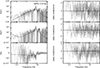 |
Fig. A.1. Same as Figure 3 but for observation ID 6557020402 when the type-C QPO centroid frequency was 7.0 Hz. |
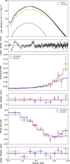 |
Fig. A.2. Same as Figure 6 but for observation ID 6557020402 with the type-C QPO at a centroid frequency 7.0 Hz. |
NICER observation log of Swift J1727.8–1613.
Figure A.3 shows corner plot of the parameters for Swift J1727 in ObsID 6203980105, fitted with the vkdualdk model. The contours represent the 1σ, 2σ, and 3σ confidence levels for pairs of parameters, while the vertical lines indicate the 1σ confidence intervals for individual parameters. Tables A.2, A.3, A.4 and A.5 give the time-averaged spectral and corona model parameters of Swift J1727 for observations 1 to 54. The rows include the observation number, QPO frequency, time lag of the QPO between the 0.5–2.0 keV and 2.0–10.0 keV bands, hydrogen column density (NH), power-law photon index of NTHCOMP (Γ), inner disc temperature (kTin), seed photon temperature of VKDUALDK (kTs, 1), sizes of the two coronae (L1 and L2), fraction of flux from the seed photon source due to feedback from the corona (η1 and η2), as well as the chi-square and degrees of freedom of the fit. Errors are given at 1σ confidence levels.
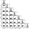 |
Fig. A.3. Corner plot for of the parameters of Swift J1727.8–1613 for ObsID 6203980105 fitted using vkdualdk. |
Time-averaged spectral and corona model parameters of Swift J1727.8–1613.
Same as Table A.2 for observation numbers 15 to 25.
Same as Table A.2 for observation numbers 26 to 36.
Same as Table A.2 for observation numbers 37 to 54.
All Tables
Representative best-fitting spectral and corona parameters for ObsID 6203980105 of Swift J1727.8–1613 using the single and dual corona model.
All Figures
|
Fig. 1. MAXI light curve of Swift J1727.8–1613 starting from 60175 MJD (August 19, 2023) in the 2–20 keV energy band in units of photons s−1 cm−2 (blue triangles; left y axis). The right y-axis shows the radio flux density in mJy from the VLA Low-band Ionosphere and Transient Experiment (VLITE) at 338 MHz (red data points, data from Peters et al. 2023), alongside RATAN-600 observations at frequencies of 4.7 GHz (cyan data points), 8.2 GHz (green data points), and 11.2 GHz (purple data points, data from Ingram et al. 2024). |
| In the text | |
|
Fig. 2. NICER hardness-intensity diagram starting from MJD 60181. The intensity is the 0.5–10.0 keV count rate and the hardness is the ratio of the count rate in the 5–10 keV band to that in the 0.5–2.0 keV band, with data points binned over 100 seconds. The colour scale indicates the MJD. |
| In the text | |
|
Fig. 3. Top left panel displays the 0.5–10.0 keV power density spectrum of Swift J1727.8–1613, fitted with five Lorentzians for ObsID 6203980105. The middle and bottom left panels show the real and imaginary parts of the cross spectrum between the 0.5–2.0 keV and 2.0–10.0 keV bands, along with the best-fitting model that assumes that the phase lags of each Lorentzians are constant with Fourier frequency (see Méndez et al. 2024). The right-hand panels display the residuals of the fits for the respective spectra. |
| In the text | |
|
Fig. 4. QPO frequency of Swift J1727.8–1613 as a function of MJD. The colour bar gives the QPO fractional RMS amplitude in the 0.5–10.0 keV energy range. |
| In the text | |
|
Fig. 5. Phase-lag spectra corresponding to specific QPO frequencies, from 0.34 Hz to 7.02 Hz. The reference energy band used here for the lags is 0.5–10.0 keV. |
| In the text | |
|
Fig. 6. Top panel shows the NICER time-averaged spectrum of Swift J1727.8–1613 (ObsID 6203980105) with a QPO centroid frequency of 0.89 Hz, fitted using the model TBfeo*(diskbb + gaussian + nthComp) together with the residuals of the best-fitting model. The middle panel shows the RMS spectrum of the QPO fitted with the vkdualdk*dilution (red) and vkompthdk*dilution (blue) models with the residuals of the best-fitting model. The bottom panel shows the phase-lag spectrum of at the QPO fitted with the vkdualdk (red) and vkompthdk model (blue) with the residuals of the best-fitting model. The 0.5–10.0 keV energy band is used as the reference for the phase-lag spectra. |
| In the text | |
|
Fig. 7. Top left panel shows the inner disc temperature, kTin, and coronal seed temperature, kTs, 1, as a function of time for Swift J1727.8–1613. The top right panel presents the power-law photon index of NTHCOMP, Γ, as a function of time. The bottom left panel displays the time evolution of the intrinsic feedback fraction, ηint, 1 and ηint, 2, obtained from the fit with the vkdualdk model. The bottom right panel shows the evolution of the inner disc radius (in units of gravitational radii) for inclination angles of 60° (blue) and 30° (black). For the calculation of the inner disc radius, we used a spectral hardening factor Tcol/Teff of 1.7, assumed a M⊙ black hole, and set the distance to the source at 2.7 kpc. |
| In the text | |
|
Fig. 8. Evolution of the sizes of the coronas, L1 and L2, for Swift J1727.8–1613 using the vkdualdk model. The right y axis shows the radio flux density in mJy obtained from the VLA Low-band Ionosphere and Transient Experiment (VLITE) at 338 MHz (red data points, data from Peters et al. 2023), alongside RATAN-600 observations at frequencies of 4.7 GHz (cyan data points), 8.2 GHz (green data points), and 11.2 GHz (purple data points, data from Ingram et al. 2024). |
| In the text | |
|
Fig. A.1. Same as Figure 3 but for observation ID 6557020402 when the type-C QPO centroid frequency was 7.0 Hz. |
| In the text | |
|
Fig. A.2. Same as Figure 6 but for observation ID 6557020402 with the type-C QPO at a centroid frequency 7.0 Hz. |
| In the text | |
|
Fig. A.3. Corner plot for of the parameters of Swift J1727.8–1613 for ObsID 6203980105 fitted using vkdualdk. |
| In the text | |
Current usage metrics show cumulative count of Article Views (full-text article views including HTML views, PDF and ePub downloads, according to the available data) and Abstracts Views on Vision4Press platform.
Data correspond to usage on the plateform after 2015. The current usage metrics is available 48-96 hours after online publication and is updated daily on week days.
Initial download of the metrics may take a while.