| Issue |
A&A
Volume 706, February 2026
|
|
|---|---|---|
| Article Number | A230 | |
| Number of page(s) | 18 | |
| Section | Interstellar and circumstellar matter | |
| DOI | https://doi.org/10.1051/0004-6361/202556767 | |
| Published online | 16 February 2026 | |
A global view on star formation: The GLOSTAR Galactic plane survey
XII. Effelsberg’s continuum view and data release
1
Max-Planck-Institut für Radioastronomie,
Auf dem Hügel 69,
53121
Bonn,
Germany
2
Purple Mountain Observatory, Chinese Academy of Sciences,
10 Yuanhua Road,
Nanjing
210023,
PR China
3
National Radio Astronomy Observatory,
PO Box O,
Socorro,
NM
87801,
USA
4
Center for Astrophysics | Harvard & Smithsonian,
60 Garden Street,
Cambridge,
MA
02138,
USA
5
Centre for Astrophysics and Planetary Science, University of Kent,
Canterbury
CT2 7NH,
UK
6
National Astronomical Observatories, Chinese Academy of Sciences,
Beijing
100101,
China
7
Key Laboratory of Radio Astronomy and Technology, Chinese Academy of Sciences,
A20 Datun Road, Chaoyang District,
Beijing
100101,
PR China
8
Instituto Nacional de Astrofísica, Óptica y Electrónica,
Apartado Postal 51 y 216,
72000
Puebla,
Mexico
9
I. Physikalisches Institut, Universität zu Köln,
Zülpicher Str. 77,
50937
Köln,
Germany
10
Max Planck Institute for Astronomy,
Königstuhl 17,
69117
Heidelberg,
Germany
11
Department of Earth and Space Science, Indian Institute for Space Science and Technology,
Trivandrum
695547,
India
12
Department of Physics, Indian Institute of Science,
Bengaluru
560012,
India
13
Laboratoire d’astrophysique de Bordeaux, Univ. Bordeaux, CNRS,
B18N, allée Geoffroy Saint-Hilaire,
33615
Pessac,
France
★ Corresponding author: This email address is being protected from spambots. You need JavaScript enabled to view it.
Received:
6
August
2025
Accepted:
15
December
2025
Abstract
Context. Extended radio continuum emission and its linear polarization play a key role in probing large-scale structures of synchrotron and free-free emission in the Milky Way. Despite the existence of many radio continuum surveys, sensitive, high-angular-resolution single-dish surveys of extended radio continuum emission remain scarce.
Aims. Our objective is to deliver a Galactic plane survey of extended radio continuum emission within the 4–8 GHz frequency range, achieving an unprecedented angular resolution of ≲3′. As part of the GLObal view of STAR formation (GLOSTAR) survey, we also crucially complement existing data from the Karl G. Jansky Very Large Array (VLA) by addressing the missing zero-spacing gap.
Methods. Within the framework of the GLOSTAR Galactic plane survey, we performed large-scale radio continuum imaging observations toward the Galactic plane in the range −2° < ℓ < 60° and |b| < 1.1°, as well as the Cygnus X region (76° < ℓ < 83° and −1° < b < 2°) with the Effelsberg 100-m Radio Telescope.
Results. We present the Effelsberg continuum survey at 4.89 GHz and 6.82 GHz, including linear polarization, with angular resolutions of 145′′ and 106′′, respectively. The survey has been corrected for missing large-scale emission using available low-angular-resolution surveys. Comparison with previous single-dish surveys indicates that our continuum survey represents the highest-quality single-dish data collected to date at this frequency. More than 90% of the flux density missed by the VLA D-array data is effectively recovered by the Effelsberg continuum survey. The improved sensitivity and angular resolution of our survey enable reliable mapping of Galactic magnetic field structures, with polarization data less affected by depolarization than in previous surveys. The GLOSTAR single-dish continuum data will be released publicly, offering a valuable resource for studying extended objects including HII regions, supernova remnants, diffuse interstellar medium, and Galactic structure.
Key words: surveys / HII regions / ISM: supernova remnants / galaxies: general / radio continuum: general / radio continuum: ISM
Jansky Fellow of the National Radio Astronomy Observatory.
Deceased.
© The Authors 2026
 Open Access article, published by EDP Sciences, under the terms of the Creative Commons Attribution License (https://creativecommons.org/licenses/by/4.0), which permits unrestricted use, distribution, and reproduction in any medium, provided the original work is properly cited.
This article is published in open access under the Subscribe to Open model.
Open Access funding provided by Max Planck Society.
1 Introduction
Ionized gas constitutes a significant component of the interstellar medium (ISM), accounting for ∼20% of the total gas mass within the Milky Way (e.g., Tielens 2010; Draine 2011). This component fills the gaps between the colder and denser phases of the ISM, namely the cold and warm neutral media (CNM and WNM). Widespread throughout the Galactic plane, ionized gas exerts a critical influence on the Galaxy’s dynamics, energy balance, and overall structure. Therefore, investigating the properties of the Galactic ionized gas is essential for a comprehensive understanding of the physical processes of star formation, HII regions, supernova remnants (SNRs), stellar feedback, and Galactic structures.
Radio continuum surveys are indispensable for studying ionized gas in the Milky Way, detecting both nonthermal synchrotron and thermal bremsstrahlung (i.e., free-free) radiation from electrons in ionized gas (e.g., Wilson et al. 2013; Condon & Ransom 2016). These emissions, prominent at centimeter wavelengths, can penetrate dust clouds that obscure observations at optical wavelengths, providing an unobstructed view of the ionized ISM.
A large number of single-dish and interferometric radio continuum surveys have already been carried out to study the Galactic plane (e.g., Reich et al. 1984; Condon et al. 1998; Beuther et al. 2016; Padmanabh et al. 2023). While interferometric radio continuum observations provide a high-angular-resolution view of the radio continuum emission, the missing short spacings in the uv-space make these observations insensitive to large-scale radio continuum structures (see Fig. 1 in Medina et al. 2019). Combining single-dish and interferometric data enables a Galactic plane survey to capture continuum and polarized emission structures across all angular scales larger than the interferometer’s angular resolution (Landecker et al. 2010; Wang et al. 2020; Brunthaler et al. 2021; Dokara et al. 2023). Hence, single-dish radio continuum surveys are important for recovering the large-scale radio continuum structure.
Single-dish radio continuum studies of the Milky Way date back to the pioneering work of Reber (1944). Existing radio continuum Galactic plane surveys with angular resolutions of 20′ or better – conducted with ground-based single-dish telescopes – span frequencies from around 1 GHz up to 10 GHz (Altenhoff et al. 1970; Condon et al. 1989; Reich et al. 1990a; Fürst et al. 1990; Reich et al. 1990b; Handa et al. 1987; Sun et al. 2011b; Irfan et al. 2015; Sun et al. 2025). Space telescopes such as the Wilkinson Microwave Anisotropy Probe (WMAP) and the Planck space telescope cover higher frequencies than ~23 GHz (Page et al. 2007; Planck Collaboration I 2020). However, all single-dish radio continuum surveys have angular resolutions of ≳2.′7, indicating a scarcity of high-angular-resolution single-dish radio continuum surveys. Our Effelsberg radio continuum survey aims to address this gap, achieving an angular resolution of ≲2.′4. While the angular resolution of our survey is similar to the early Effelsberg 5 GHz survey by Altenhoff et al. (1979), the survey sensitivity will be significantly enhanced, thanks to advancements in receiver system technology.
As part of the Global View on Star Formation in the Milky Way (GLOSTAR1) survey (Medina et al. 2019; Brunthaler et al. 2021), we conducted large-scale radio continuum imaging observations of the Galactic plane at 4–8 GHz with the Effelsberg 100-m Radio Telescope. These observations complement the Karl G. Jansky Very Large Array (VLA) survey, enhancing our study of Galactic structures on all scales down to ~1′′. The GLOSTAR data have already been used in a wide range of studies. These include the compilation of catalogs of compact radio continuum sources (Medina et al. 2019; Dzib et al. 2023; Yang et al. 2023; Medina et al. 2024) and the estimation of the present-day star formation rate in the central molecular zone (Nguyen et al. 2021). The data have also been employed to study radio recombination line (RRL) emission from bright HII regions (Khan et al. 2024), to identify the youngest HII regions, examine their variability (Yang et al. 2025), and characterize SNRs (Dokara et al. 2021, 2023). In addition, GLOSTAR has enabled searches for 6.7 GHz class II CH3OH masers (Ortiz-León et al. 2021; Nguyen et al. 2022) and investigations of 4.8 GHz formaldehyde absorption in Cygnus X (Gong et al. 2023). The Effelsberg radio continuum component of the GLOSTAR survey will allow us to explore the large-scale radio continuum structures in the Milky Way.
Although smaller portions of our Effelsberg radio continuum observations, combined with the VLA observations, have been previously reported (e.g., Brunthaler et al. 2021; Dokara et al. 2023; Gong et al. 2023), these studies are limited to specific regions. Here, we extend this research by investigating the properties of radio continuum emission in the Galactic plane, providing insights into the characteristics on a Galactic scale.
Observations and data reduction are described in Sect. 2. Subsequently, observational results and discussion are presented in Sect. 3. Our findings are summarized in Sect. 4.
2 Observations and data reduction
2.1 Observations with the Effelsberg 100 m telescope
As an important component of the GLOSTAR survey (Brunthaler et al. 2021), we performed large-scale 4–8 GHz radio continuum observations using the Effelsberg 100-m Radio Telescope2. The observed regions include the Galactic plane in the range −2° < ℓ < 60° and |b| < 1.1°, as well as the Cygnus X region (76° < ℓ < 83° and −1° < b < 2°). These observations were carried out between 2019 January 11 and 2023 August 23 (project codes 102-20 and 22-15). Our observations have a sky coverage of ∼145 square degrees in total. Although the continuum and spectral-line observations were conducted simultaneously, here we focus on the continuum and polarization observations. For the continuum observations, the SPEctro-POLarimeter (SPECPOL) backend was used to record the full Stokes continuum emission in the MBFITS format3. SPECPOL offers two frequency bands, spanning 4–6 GHz (lower band) and 6–8 GHz (upper band), respectively. Each band is divided into 1024 channels, yielding a channel width of 1.95 MHz.
For observations, the Galactic plane in the range −2° < ℓ < 60° and |b| < 1.1° was split into 31 fields4, while the Cygnus X region was split into three fields. In the pilot region (28° < ℓ < 36° and |b| < 1°), each field was divided into rectangular cells of 0.2°×2° (Brunthaler et al. 2021). In Cygnus X, each field was divided into 0.1°×3° cells. The rest of the fields were divided into rectangular cells of 0.2°×2.2°. These cells facilitate flexible observing schedules. Before the observations began, the high-speed analog-to-digital converters (ADCs) were calibrated to minimize offset, gain, and phase (OGP) variations within each converter in a procedure similar to that in Patel et al. (2014). Following the OGP corrections, the time delay between the two signal paths were measured by computing the correlation of a common noise source fed to the ADCs. Subsequently, this delay was compensated for in the SPECPOL firmware by delaying one of the signals appropriately before computing the Stokes parameters. The on-the-fly (OTF) mode was used to map each cell with a scanning speed of 90′′ per second and a step of 30′′to fulfill the Nyquist sampling condition. Each region was mapped in both Galactic longitude and latitude to enable basket weaving and suppress the scanning artifacts (e.g., Müller et al. 2017). During the observations, system temperatures were typically 28–42 K. Focus was verified after sunrise and sunset. Nearby pointing observations were carried out every 2–3 hours. The rms pointing uncertainty was found to be within 10′′.
The calibrators 3C 286 and NGC 7027 were observed to derive accurate bandpass solutions and compute the calibration fit for the SPECPOL data (Ott et al. 1994; Brunthaler et al. 2021; Perley & Butler 2013, 2017). The calibration of the Stokes parameters (I, U, Q) was performed by applying the Müller matrix (e.g., Heiles et al. 2001) obtained by observing 3C 286 at different parallactic angles. To minimize radio-frequency interference (RFI) in the raw continuum data, we selected discontinuous channels centered at 4.89 GHz and 6.82 GHz, respectively, to produce the radio continuum images (see Fig. A.1). These channels cover a bandwidth of ~120 MHz at both frequencies. The narrow bandwidth also helps reduce the depolarization effects. According to maps of the unpolarized source 3C 295 (see Fig. A.2), the “on-axis” instrumental polarization reaches up to 0.5% in both continuum bands but higher within the “butterfly-shaped” response within the main-beam area. This calibration was further validated by mapping 3C 286 at various parallactic angles. The resulting polarization angle agrees within 1° uncertainty, and the polarization fraction is consistent to within 1% uncertainty, confirming the robustness of our calibration. Based on Gaussian fitting of unresolved continuum sources, we measured the half-power beam widths (HPBWs) to be 145′′ and 106′′ at 4.89 GHz and 6.82 GHz, respectively. The observations for the region at 22° < ℓ < 26° were significantly affected by geostationary satellites. To minimize the impact of RFI during satellite passages, this region was observed multiple times, with only apparently “clean” sub-scans selected for subsequent analysis. The radio continuum data were reduced with the toolbox program and the NOD3 software package (Müller et al. 2017).
Since the radio continuum emission is prevalent throughout the observed region, the rms noise levels are difficult to determine directly from the Stokes I map. We made use of the constrained diffusion decomposition (CDD) method5 to decompose the Stokes I map (Li 2022). We estimated the noise from the most compact component, where extended emission was effectively removed and only a few compact sources remained. We applied the statistics of the emission-free area to estimate the rms noise in each field, and present the derived noise distribution in Fig. A.3. The noise levels are 3.9–11.5 mK (i.e., 1.6–4.7 mJy beam−1) in the lower band and 3.2–8.9 mK (i.e., 1.4–3.8 mJy beam−1) in the upper band. The noise distribution is similar for both bands, with slightly higher levels observed in the lower band. For polarized emission, we see a similar decrease in noise with increasing Galactic longitude with a median value of about 7 mK at both frequencies. Additionally, elevated noise levels near the Galactic center arise from observations conducted at low elevations. The observational parameters of this continuum survey are summarized in Table 1.
2.2 Zero-level restoration
Due to the limited latitude coverage of our observations, the zero level is not reached, having offsets from the absolute zero level in the reduced radio continuum images. Similar to our previous efforts (Brunthaler et al. 2021; Gong et al. 2023), the zero-level intensities of our Effelsberg data requires restoration.
While the restoration for the Cygnus X region was performed in Gong et al. (2023), the Galactic plane in the range 2° < ℓ < 60° and |b| < 1° remains uncorrected. For 10° < ℓ <− 60°, we used the Urumqi 4.8 GHz continuum data (Sun et al. 2007, 2011b). Since these data do not cover −2° < ℓ < 10°, we instead used the Parkes 5 GHz data from the southern hemisphere survey of the Galactic plane (Haynes et al. 1978) for restoration in this region. Both the Urumqi and Parkes survey data were taken from the MPIfR’s Survey Sampler6. These surveys cover overlapping regions, enabling intensity comparisons. We convolved both datasets to a common HPBW of 15′for comparison, as we only used these for large-scale restoration.
We compare the two datasets within 10° < ℓ < 30° in Fig. A.4. In Fig. A.4a, we notice that the brightness temperatures of the Parkes survey data are generally consistent with those of the Urumqi survey except for bright compact sources. Figure A.4b suggests that most of the temperature differences lie between 0 K and 0.1 K with a median value of 0.028 K. We also observe that the temperature difference varies with Galactic latitude, as demonstrated for a Galactic longitude of ℓ = 11.°65 (see Fig. A.4c). The Galactic longitude at ℓ = 11.°65 was selected as it is predominantly characterized by extended emission and largely free of bright compact emissions. To mitigate this large-scale variation, we applied a third-order polynomial fit to the Galactic-latitude-dependent variation. The fitting result was subsequently applied to the Parkes 5 GHz data within −2° < ℓ < 10°, which effectively matches the intensity scale between the two datasets. Finally, we combined the Urumqi data and the corrected Parkes data to provide a template of the large-scale distribution (see Fig. C.1 in Appendix C).
Following our previous studies (Brunthaler et al. 2021; Gong et al. 2023), we restored the zero-level distribution of the GLOSTAR 4.89 GHz continuum data using the large-scale template derived from the Urumqi and Parkes surveys. The restored Effelsberg 4.89 GHz continuum data were convolved to the Urumqi survey’s HPBW (9′.5)for comparison, as shown in Fig. A.5. A linear fit to the observed data points reveals the brightness temperature of the Urumqi survey to be ~97.4% of that of the GLOSTAR survey, indicating good agreement between the two surveys within 4%.
For the polarization data, corrections for zero-level offsets and baseline distortions are required. Unlike Stokes I, Stokes Q and U maps can contain negative values, rendering the background filtering method (Sofue & Reich 1979) used for the Stokes I maps unsuitable. Instead, we applied a modified version of this method (Kothes & Kerton 2002) that accounts for positive and negative intensity values. For ℓ > 10°, zero-level offsets were restored using Urumqi polarization data, while for ℓ < 10° we utilized the nine-year WMAP K-band data (Bennett et al. 2013). We separated small- and large-scale components at 90′ angular resolution in both the GLOSTAR and the WMAP maps. The large-scale WMAP component was scaled assuming a brightness temperature spectral index of β = −2.9 (Reich & Reich 1988) and added to the GLOSTAR maps. Figure A.6 presents the zero-restoration of the GLOSTAR 4.89 GHz polarization data in the Galactic center. The plot indicates that the large-scale Stokes U and Q distributions have been successfully corrected, while the small-scale structures remain nearly identical to the original ones. Hence, this approach effectively corrects zero-level offsets and mitigates baseline distortions in the Effelsberg polarization maps
Observational parameters of the Effelsberg continuum survey.
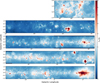 |
Fig. 1 Effelsberg 4.89 GHz Stokes I continuum map of the entire GLOSTAR survey. Zoom-in plots of each fields are available via https://gongyan2444.github.io/glostar-snr-hii.html, where the green, gray, and red circles represent the known SNRs (Green 2025), SNR candidates (Anderson et al. 2017; Dokara et al. 2021; Anderson et al. 2025), and HII regions from the WISE catalog (Anderson et al. 2014), respectively. |
3 Results and discussion
3.1 Overall distribution
Figures 1 and 2 show the Effelsberg 4.89 GHz and 6.82 GHz Stokes I data from the GLOSTAR survey. The overall distributions of Stokes I continuum emissions closely resemble those observed in early radio continuum images (e.g., Altenhoff et al. 1970; Haynes et al. 1978; Reich et al. 1990a,b; Sun et al. 2007, 2011b) but with higher angular resolution. The bulk of the bright emission is confined near the Galactic midplane and declines rapidly with increasing latitude (see the scale-height analysis in Appendix B), indicating that it predominantly traces structures within the Galactic disk. Numerous extended structures are evident throughout the maps. The brightest among them correspond to well-known HII regions and SNRs, which contribute to the thermal and nonthermal emission budgets, respectively (see Sect. 3.4 for a detailed discussion). These sources also play a role in shaping the observed asymmetry of the latitude profile (see Appendix B). Beyond these classical sources, the Effelsberg data also capture a variety of large-scale structures. These include, for example, the prominent bipolar radio chimney in the Galactic center, which extends to ∼430 pc above the midplane (e.g. Heywood et al. 2019; Veena et al. 2023), as well as the bright and extended radio continuum emission associated with the Galaxy’s major mini-starburst regions, such as Sgr B2, W43, and W51. In addition to these prominent objects, the Effelsberg data also reveal a wealth of compact extragalactic point sources, filaments, and diffuse features that contribute to the complex radio continuum landscape of the Galactic plane.
To highlight the improvement in image fidelity of the GLOSTAR data compared to previous surveys at similar frequencies (Haynes et al. 1978; Condon et al. 1989; Sun et al. 2007), we show the Stokes I continuum maps from different surveys in Fig. 3. Owing to the higher angular resolution and sensitivity, our GLOSTAR data reveal significantly finer structures and a higher number of faint sources compared to the Urumqi (Sun et al. 2007), Green Bank 6 cm7 (GB6; Condon et al. 1989), and Parkes (Haynes et al. 1978) radio continuum surveys at ∼5 GHz. Furthermore, our data exhibit fewer image artifacts than the Parkes continuum map, where scanning effects are evident (see the lower left panel of Fig. 3). The GB6 survey data suffer from zero-level offsets and uncorrected large-scale distortions, resulting in extensive regions of negative values in the survey map (see the lower middle panel of Fig. 3). These issues arise from the baseline subtraction method adopted in the GB6 survey (Condon et al. 1989), which tends to suppress extended emission. This comparison demonstrates that the GLOSTAR radio continuum data are currently the highest-quality single-dish continuum data in this frequency range.
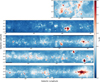 |
Fig. 2 Effelsberg 6.82 GHz Stokes I continuum map of the entire GLOSTAR survey. |
3.2 Missing flux: The importance of the Effelsberg 100 m observations
One of the main goals of the Effelsberg radio continuum survey is to recover the missing flux in the radio interferometry data of the GLOSTAR survey, which lack zero-spacing information. Given that our VLA observations have shortest baselines of ∼30 m (see Fig. A.7, for instance), our Effelsberg 100 m observations can perfectly fill the missing zero-spacing gap in the uv-plane.
We use the Stokes I continuum distribution of the Galactic center to illustrate the improvement incorporating the Effelsberg 100 m data. As shown in Fig. 4a (see also Fig. 1 in Nguyen et al. (2021)), our VLA D configuration data have a maximum recoverable scale of ∼4′, resulting in a fragmented image. This fragmentation arises because the data primarily capture compact features, while the broader, diffuse emission is not adequately sampled in the VLA D configuration observations. To mitigate this issue, we combined the Effelsberg 100 m data with the VLA D configuration data following Dokara et al. (2023). The resulting image, displayed in Fig. 4b, presents a smooth, continuous distribution that reveals the full extent of the structure across all angular scales above ∼18′′– the angular resolution of the combined data. Consequently, the brightness distribution more accurately traces extended sources in the Galactic plane.
We constructed the angular power spectra for both datasets to examine the distribution of power across different angular scales. The resulting spectra toward the Galactic center are presented in Fig. 5a. The two power spectra agree well on angular scales ≲2′. On larger scales, however, the VLA-only image shows a slight power deficit relative to the VLA-Effelsberg combined image. This indicates that, despite the nominal ∼4′ largest angular scale of the D-array, the practical sensitivity to diffuse emission is reduced because of sparse short-baseline coverage and snapshot uv sampling. Compared with the VLA-only image, the spatial power spectrum of the VLA-Effelsberg combined image is better described by a single power-law distribution on angular scales of ≳1′, showing that the power of the ionized gas decreases toward smaller angular scales. A linear fit to the data for angular scales >100′′ yields a power index of about −2.3, which is slightly shallower than the 2D Kolmogorov-like spectral index of −8/3 predicted for isotropic, incompressible turbulence (Kolmogorov 1941). Previous studies indicate that electron density fluctuations associated with interstellar turbulence are likely to follow a Kolmogorov-like spectrum (Armstrong et al. 1995), which describes an energy cascade from large to small scales. The slightly flatter spectrum observed here may indicate the non-negligible contribution of small-scale turbulence to the overall spectrum (Lazarian & Pogosyan 2000).
Using the integrated flux densities over each field (see Sect. 2) in both VLA-only and VLA-Effelsberg combined images, we estimated the total flux density and thereby quantified the percentage of flux density missed by the VLA data. Comparing the derived values in Fig. 5b, we find that nearly all fields miss more than 90% of flux densities in the VLA D array images. This highlights the crucial role of the Effelsberg 100 m observations in recovering the extended emission for the GLOSTAR survey.
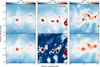 |
Fig. 3 Comparison of the Effelsberg 4.89 GHz Stokes I continuum map with maps from the Urumqi, GB6, and Parkes surveys at similar frequencies. |
3.3 Polarization
Polarization data from radio continuum observations provide valuable insights into magnetic field structures in astrophysical objects. Figures 6 and 7 present the Effelsberg 4.89 GHz and 6.82 GHz full Stokes data from the GLOSTAR survey. Compared to previous polarized continuum surveys at similar frequencies (Sun et al. 2007; Jew et al. 2019), our Effelsberg polarization data provide at least a threefold improvement in angular resolution.
Consistent with previous polarization surveys (e.g. Sun et al. 2007), our observations reveal widespread diffuse polarized structures that often lack corresponding counterparts in Stokes I. This effect is particularly pronounced toward the inner Galaxy, where the polarized emission becomes highly patchy. Two main classes of mechanisms have been proposed to explain such behavior (e.g. Sun et al. 2014): (i) intrinsically irregular emission produced in regions dominated by random magnetic fields (e.g. Sun et al. 2011b), and (ii) the modulation of a smooth background by foreground Faraday screens. The latter may arise from either MHD turbulence within the warm ionized medium (Gaensler et al. 2011) or discrete ionized structures such as HII regions (Gaensler et al. 2001; Sun et al. 2011b). In our data (e.g., near ℓ ∼ 9°; see Figs. 6 and 7), the polarized emission appears more fragmented at 4.89 GHz than at 6.82 GHz, consistent with stronger depolarization at the lower frequency and thus supporting the foreground-screen scenario. Nevertheless, dedicated studies will be required to robustly quantify the underlying mechanisms and to constrain the physical origin of these depolarizing structures.
From our data, we detect prominent polarization structures in at least 30 SNRs and SNR candidates. For five sources (e.g., G8.8583−0.2583, G21.0−0.4, G22.7−0.2, G26.75+0.73, and G54.4−0.3), which previously showed −polarization only in VLA D-array data (Dokara et al. 2021), our Effelsberg observations deliver the first single-dish detections of polarization. Although the VLA data reveal small-scale polarized structures, they are insensitive to the extended polarized emission filtered out by the interferometer. Our Effelsberg measurements therefore play a crucial role in recovering large-scale polarization. Even for SNRs with earlier polarization measurements at lower frequencies, our observations offer improved constraints on the intrinsic polarization structures (see Sect. 3.4.2, for instance). In addition, our observations reveal extended polarization structures that lack corresponding features in Stokes I, in agreement with previous polarization surveys (e.g., Sun et al. 2007). Such “polarization-only” features are commonly attributed to diffuse Galactic synchrotron emission, with their morphology and visibility shaped by Faraday rotation and depolarization effects along the line of sight.
We note that instrumental polarization has not been completely removed from the polarization images (see Sect. 2.1 for details on the instrumental polarization measurements). For example, a source with a brightness temperature of Tb = 1 K can contribute up to 10 mK to the polarized intensity maps, assuming an instrumental polarization level of 1%. Consequently, leakage from bright HII regions may introduce a bias in the polarization measurements. By cross-checking the Stokes I and polarization images, we identified a few HII regions where such contamination may significantly affect the polarization results. These include G005.887−00.443, G008.137+00.232, W31, G010.308−00.150, W33, G013.880+00.285, M16, G018.144−00.281, G019.609−00.239, M17, G020.728−00.105, G023.957+00.149, G025.382−00.151, G29, W43, G032.800+00.190, NRAO584, G037.763−00.212, W47, W49, G045.121+00.133, K47, W518, S106, DR7,− DR15, DR22, and DR21. We therefore caution that the polarization analysis in these regions should be interpreted with care.
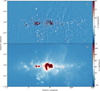 |
Fig. 4 Comparison of GLOSTAR data with and without incorporating the Effelsberg data at 5.8 GHz. (a) VLA D-array only continuum image. (b) Combination of VLA D-array and Effelsberg 100 m single-dish images. |
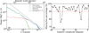 |
Fig. 5 (a) Angular power spectra of the VLA-D array, Effelsberg-100 m, and VLA-Effelsberg combined images toward the representative region near the Galactic center (see Fig. 4). The 2D Kolmogorov-like spectrum is indicated by the dashed black line for comparison. (b) Percentage of missing flux of the VLA D-array data across the Galactic plane covered by the GLOSTAR survey. The horizontal dashed red line indicates a missing flux fraction of 10%. |
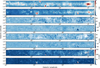 |
Fig. 6 Distribution of the Stokes I, Q, U, and polarization intensity maps from the Effelsberg 4.89 GHz continuum emission of the GLOSTAR survey. Zoom-in plots of each fields are available via https://gongyan2444.github.io/glostar-snr-hii.html, where the green, gray, and red circles represent the known SNRs (Green 2025), SNR candidates (Anderson et al. 2017; Dokara et al. 2021; Anderson et al. 2025), and HII regions from the WISE catalog (Anderson et al. 2014), respectively. |
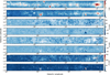 |
Fig. 7 Distribution of the Stokes I, Q, U, and polarization intensity maps from the Effelsberg 6.82 GHz continuum emission of the GLOSTAR survey. |
3.4 Extended objects
As shown in the online version of Fig. 1, the GLOSTAR data encompass 99 known SNRs (Green 2025), 241 SNR candidates (Anderson et al. 2017; Dokara et al. 2021; Anderson et al. 2025), and 3633 HII regions from the WISE catalog (Anderson et al. 2014), suggesting that discrete radio continuum sources are dominated by SNRs and HII regions in the Galactic plane. HII regions emit thermal free-free radiation from ionized gas surrounding young massive stars. In contrast, SNRs are typically characterized by nonthermal synchrotron emission. The morphology and spectral index derived from radio continuum observations provide key diagnostics of the physical conditions and evolutionary stages of both HII regions and SNRs, while the magnetic-field structure inferred from polarization measurements offers additional insights into the latter. The GLOSTAR Effelsberg survey thus provides a valuable dataset for detailed investigations of the nature and properties of these populations. In the following, we present case studies of representative examples from each category to demonstrate the excellent capability of the Effelsberg data.
3.4.1 HII regions
We selected G016.648−00.357 (also known as Sh 2-48) as a representative case to demonstrate our analysis methodology toward an HII region. At a distance of 3.8 kpc (e.g., Ortega et al. 2013; Torii et al. 2021), this evolved HII region is extended with a radius of ∼7′ (i.e., 7.7 pc), making our Effelsberg data more suitable for analysis compared to the GLOSTAR VLA observations.
Figure 8a presents the radio continuum distribution of this region, which exhibits a cometary morphology, with a bright head located toward the northwest and a diffuse tail extending toward the southeast. No polarized emission is detected in this region. To constrain the spectral index9, we employed a temperature–temperature (TT) plot, which is not affected by zero-level uncertainties in the images (e.g., Turtle et al. 1962). The TT plot, shown in Fig.8b, reveals a linear relation between the radio continuum emission at 4.89 GHz and 6.82 GHz, with a high Pearson correlation coefficient of 0.997. A linear fit to the observed data yields a brightness temperature spectral index of β = −2.06 ± 0.05, consistent with an optically thin spectral index for HII regions (e.g., Gao et al. 2019). This result indicates that continuum emissions at both bands are in excellent agreement with optically thin conditions.
Electron temperatures are a fundamental parameter for characterizing the physical conditions in HII regions. Its accurate determination requires measurements of both the radio continuum and associated RRL observations. In particular, our simultaneous RRL and continuum observations enables investigations into spatial fluctuations of the electron temperature within HII regions. To derive electron temperatures, we combined our continuum maps with RRL data from the GBT Diffuse Ionized Gas Survey (GDIGS10; Anderson et al. 2021), which provides Hnα measurements at a mean frequency of 5.69 GHz and an angular resolution of 2′.65. To match this resolution, we convolved our radio continuum data at both frequencies to 2.′65. The continuum emission at 5.69 GHz was then derived by interpolating our convolved data using the brightness temperature spectral index β = −2.06. Assuming optically thin emission and adopting a main beam efficiency of 92%11 for the GDIGS data, electron temperatures, Te, were calculated following the relation (e.g., Wenger et al. 2019):
![Mathematical equation: $\left( {{{{T_{\rm{e}}}} \over {{\rm{K}}}}} \right) = {\left\{ {7100{{\left( {{v \over {{\rm{GHz}}}}} \right)}^{1.1}}\left( {{{{S_{\rm{C}}}} \over {{S_{\rm{L}}}}}} \right){{\left( {{{\Delta v} \over {{\rm{km}}{{\rm{s}}^{ - 1}}}}} \right)}^{ - 1}}{{\left[ {1 + {{n\left( {^4{\rm{H}}{{\rm{e}}^ + }} \right)} \over {n\left( {{{\rm{H}}^ + }} \right)}}} \right]}^{ - 1}}} \right\}^{0.87}}$](/articles/aa/full_html/2026/02/aa56767-25/aa56767-25-eq1.png) (1)
where
(1)
where  is the continuum-to-line ratio, ∆3 is the full width at half maximum (FWHM) line width, and n(4He+)/n(H+) is the He+/H+ abundance ratio, assumed to be 0.08 (e.g., Quireza et al. 2006; Gong et al. 2015).
The resulting distribution of electron temperatures is shown in Fig. 8c; it spans 4351 K to 7819 K, with a median of 5685 K. The associated 1σ uncertainties range from 193 K to 813 K, with a median uncertainty of 418 K. These values are slightly lower than those predicted by the Galactic electron temperature gradient (e.g., Khan et al. 2024). In this figure, elevated electron temperatures are preferentially found at the boundary of the HII region, exhibiting a gradient that decreases toward the center. Such a temperature structure is likely driven by photon hardening effects at the edges (see Figure 7.9 in Tielens 2005, for instance; Khan et al. 2022), where lower-energy photons are preferentially absorbed by neutral hydrogen due to their larger ionization cross sections, allowing higher-energy photons to penetrate further into ambient gas.
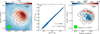 |
Fig. 8 Observed properties of G016.648−00.357 (i.e., Sh 2-48). (a) Effelsberg 4.89 GHz Stokes I image overlaid with the GDIGS RRL integrated-intensity contours. (b) TT plot between 4.89 GHz and 6.82 GHz at a common angular resolution of 2′.65. The dashed red line shows the best fit to the observed data points. (c) Spatial distribution of the derived electron temperatures overlaid with the GDIGS RRL integrated-intensity contours. In panels (a) and (c), the integrated velocity ranges from 0 to 70 km s−1 for the GDIGS RRL integrated intensity contours, starting at 1 K km s−1 and increasing by 0.5 K km s−1. The location of the exciting star BD−14 5014 is marked with a gold star. In each panel, the beam is shown in the lower-left corner, and the scale bar in the top-right corner is based on an assumed distance of 3.8 kpc (e.g., Ortega et al. 2013; Torii et al. 2021). |
3.4.2 Supernova remnant
As an example for an extended SNR from our survey, we present maps of SNR W28 (also known as G6.4−0.1), a well-known mixed-morphology SNR associated with very high-energy γ-ray sources (Aharonian et al. 2008) and a runaway pulsar (Frail et al. 1993). In particular, polarization measurements of W28 are rare, with only a few early studies available (e.g., see Fig. 9b in Kundu & Velusamy 1972 and Fig. 15 in Dickel & Milne 1976). In Fig. 9, we present a comparison of the polarization results toward W28 from the 2.695 GHz Effelsberg Galactic plane survey (Duncan et al. 1999) and our GLOSTAR survey. Strong, ordered linear polarization is detected along its radio shell at 4.89 GHz and 6.82 GHz in our GLOSTAR data, with the inferred magnetic field vectors (obtained by rotating the observed polarization vectors by 90°) oriented nearly parallel to the shell and exhibiting low dispersion in polarization position angles. This tangential distribution is consistent with the expected compression of magnetic fields by the supernova shock, a phenomenon commonly observed in evolved SNR shells (e.g., Reich et al. 1992; Fürst & Reich 2004; Han 2017). Furthermore, the tangential pattern observed in our data is more pronounced than that seen in polarization measurements from the 2.695 GHz Effelsberg Galactic plane survey (see the left panel of Fig. 9) and previous studies (Kundu & Velusamy 1972; Dickel & Milne 1976), indicating significant depolarization effects at lower frequencies.
We also employed the TT plot method to derive the spectral index of the source. W28 is known to be superimposed with several HII regions along the line of sight (e.g., Anderson et al. 2014). To minimize contamination from thermal emission, we therefore restricted our analysis to the northeastern shell to determine the spectral index. As shown in Fig. 9d, a clear linear relation is observed between the two bands, with a high Pearson correlation coefficient of 0.996. A linear fit to the data yields a brightness temperature spectral index of β =−2.59 ± 0.06 (i.e., α =−0.59 ± 0.06), which is much steeper than the α = −0.35 ± 0.18 value reported at lower frequencies (Dubner et al. 2000). This difference could be due to our choice of region, as the northeastern shell is less affected by emission from nearby HII regions compared to previous studies.
The interquartile range of the linear polarization degrees spans 6% to 10% (peaking at 15%) at 4.89 GHz and 6% to 12% (peaking at 17%) at 6.82 GHz, with both frequencies exhibiting a median value of 8%. These results indicate consistently high levels of linear polarization fractions across the two bands. According to the synchrotron theory (e.g., Wilson et al. 2013), the intrinsic degree of linear polarization of synchrotron radiation emitted by relativistic electrons spiraling in a uniform magnetic field is given by
 (2)
where α = β + 2. Adopting a brightness temperature spectral index of β = −2.59, we obtain Π0 = 70%, which is much higher than our measured values. If the reduction in the observed polarization degree is attributed to the presence of a random magnetic-field component, the observed linear polarization degree can be expressed as
(2)
where α = β + 2. Adopting a brightness temperature spectral index of β = −2.59, we obtain Π0 = 70%, which is much higher than our measured values. If the reduction in the observed polarization degree is attributed to the presence of a random magnetic-field component, the observed linear polarization degree can be expressed as
 (3)
where Hu and Hr are the uniform and random field strengths (e.g., Burn 1966), respectively. Using a median value of 8% for the observed degree of linear polarization, we can estimate the uniform-to-random field ratios,
(3)
where Hu and Hr are the uniform and random field strengths (e.g., Burn 1966), respectively. Using a median value of 8% for the observed degree of linear polarization, we can estimate the uniform-to-random field ratios,  , to be about 0.13. For a maximum Π = 15%,
  increases to 0.27. If Faraday depolarization also contributes to the reduced degree of linear polarization, the estimated
  values should be taken as lower limits.
Our survey provides polarization data at two frequency bands, enabling the determination of rotation measures (RMs). We convolved the Stokes Q and U maps from both bands to a common angular resolution of 160′′ and recalculated the polarization angles. Neglecting the nπ ambiguity arising from the indistinguishable orientation of the vector under a 180°(i.e., π) rotation, we derived the RMs directly from the polarization angles at the two frequencies. The RM map is shown in Fig. 9e. The resulting RMs range from −61.0 to 44.1 rad m−2 in the northeastern shell of W28. These values are significantly lower than those measured in the textbook mixed-morphology SNR W44 (e.g., Sun et al. 2011a; Génova-Santos et al. 2017). This may indicate lower electron densities, weaker line-of-sight magnetic fields, or differences in the Galactic RM environments.
As shown above, our results represent a significant improvement over earlier polarization studies, with GLOSTAR observations providing substantially higher quality single-dish data that trace the intrinsic polarization properties. This enhancement enables a more detailed and reliable investigation of the polarization and magnetic field structures within the Milky Way.
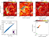 |
Fig. 9 GLOSTAR radio continuum data of W28. (a) Linear polarization intensity maps overlaid with the magnetic-field vectors from the 2.695 GHz Effelsberg Galactic plane survey. The white contours represent the 2.695 GHz Stokes I continuum emission, starting at 2.5 K and increasing in steps of 2.5 K. (b) Similar to panel a, but using GLOSTAR 4.89 GHz continuum data, with white contours starting at 1.0 K and increasing in steps of 1.0 K. (c) Similar to panel a, but based on GLOSTAR 6.82 GHz continuum data, where white contours start at 0.5 K and increase in steps of 0.5 K. In panels a–c, the polarization angles are rotated by 90° to trace the magnetic-field directions, indicated by black bars. The position of the runaway pulsar PSR B1758−23 (i.e., PSR J1801−23), thought to be associated with W28 (Frail et al. 1993), is indicated by a cyan star. In each panel, the beam is shown in the lower-left corner, and the scale bar in the top-right corner is based on an assumed distance of 2 kpc (Velázquez et al. 2002). (d) TT plot of the northeastern shell between 4.89 GHz and 6.82 GHz at a common angular resolution of 160′′. The dashed red line shows the best fit to the observed data points extracted from the region displayed in the panel in the lower right corner. (e) Distribution of the derived RMs. |
4 Summary and conclusion
As part of the GLOSTAR survey project, we presented the large-scale radio continuum observations covering the Galactic plane in the range −2° < ℓ < 60° and |b| < 1°, as well as a section in Cygnus X (76° < ℓ < 83° and −1° < b < 2°) with the Effelsberg 100-m Radio Telescope. The GLOSTAR dataset surpasses the quality of previous surveys at similar frequencies, including those from the Urumqi, Parkes, GB6, and early Effelsberg surveys. Furthermore, we showed that the Effelsberg continuum data are crucial for tracing the large-scale structure of ionized gas in the Milky Way. Our polarization data, less affected by depolarization effects compared to those at lower frequencies, offer reliable tracers of the intrinsic magnetic field orientation. These radio continuum data are freely available to the scientific community via https://glostar.mpifr-bonn.mpg.de/glostar/ and https://www.mpifr-bonn.mpg.de/ survey.html. The data are provided in FITS and other formats, facilitating their use for the investigation of extended radio continuum emission in the Milky Way. The VLA-Effelsberg combined data, which are valuable for studying extended structures with scales ≳18′′, will be released in a forthcoming publication. These valuable datasets will significantly contribute to future studies of astrophysical objects.
Data availability
The zoom-in plots of Figs. 1, 2, 6, and 7 are available via https://gongyan2444.github.io/glostar-snr-hii.html.
Acknowledgements
During the preparation of this article, we suffered the tragic loss of Prof. Karl M. Menten, the principal investigator of the GLOSTAR survey. We dedicate this work to his enduring legacy. Karl’s insight and vision shaped not only this project but also the field of radio astronomy at large. We are deeply indebted to the countless discussions with him that have inspired generations of radio astronomers. We will always miss his warmth, wisdom, boundless curiosity, generosity of spirit, kindness, and delightful sense of humor. We thank the Effelsberg 100-m telescope staff for their assistance with our observations. YG was supported by the Ministry of Science and Technology of China under the National Key R&D Program (Grant No. 2023YFA1608200), the National Natural Science Foundation of China (Grant No. 12427901), and the Strategic Priority Research Program of the Chinese Academy of Sciences (Grant No. XDB0800301). AYY acknowledges the support from the National Key R&D Program of China No. 2023YFC2206403 and National Natural Science Foundation of China (NSFC) grants Nos. 12303031 and 11988101. S.A.D. acknowledges the M2FINDERS project from the European Research Council (ERC) under the European Union’s Horizon 2020 research and innovation programme (grant No. 101018682). G.N.O.L. acknowledges the financial support provided by Secretaría de Ciencia, Humanidades, Tecnología e Innovación (Secihti) through grant CBF-2025-I-201. HB acknowledges support from the European Research Council under the Horizon 2020 Framework Programme via the ERC Consolidator Grant CSF-648505. HB also acknowledges support from the Deutsche Forschungsgemeinschaft in the Collaborative Research Center (SFB 881) “The Milky Way System” (subproject B1). YG thanks Tess Jaffe for her helpful discussion of the GB6 image from the SkyView website. This work is based on observations with the 100-m telescope of the MPIfR (Max-Planck-Institut für Radioastronomie) at Effelsberg. The National Radio Astronomy and Green Bank Observatory are facilities of the National Science Foundation operated under cooperative agreement by Associated Universities, Inc. This research has made use of NASA’s Astrophysics Data System. This work also made use of Python libraries including Astropy12 (Astropy Collaboration 2013), NumPy13 (van der Walt et al. 2011), SciPy14 (Jones et al. 2001), Matplotlib15 (Hunter 2007), LMFIT (Newville et al. 2014), and APLpy (Robitaille & Bressert 2012). The continuum view of the Effelsberg survey is also available as a movie at https://gongyan2444.github.io/movie/GLOSTAR_movie.m4v.
References
- Aharonian, F., Akhperjanian, A. G., Bazer-Bachi, A. R., et al. 2008, A&A, 481, 401 [NASA ADS] [CrossRef] [EDP Sciences] [Google Scholar]
- Altenhoff, W. J., Downes, D., Goad, L., Maxwell, A., & Rinehart, R. 1970, A&AS, 1, 319 [Google Scholar]
- Altenhoff, W. J., Downes, D., Pauls, T., & Schraml, J. 1979, A&AS, 35, 23 [Google Scholar]
- Anderson, L. D., Bania, T. M., Balser, D. S., et al. 2014, ApJS, 212, 1 [Google Scholar]
- Anderson, L. D., Wang, Y., Bihr, S., et al. 2017, A&A, 605, A58 [NASA ADS] [CrossRef] [EDP Sciences] [Google Scholar]
- Anderson, L. D., Luisi, M., Liu, B., et al. 2021, ApJS, 254, 28 [NASA ADS] [CrossRef] [Google Scholar]
- Anderson, L. D., Camilo, F., Faerber, T., et al. 2025, A&A, 693, A247 [NASA ADS] [CrossRef] [EDP Sciences] [Google Scholar]
- Armstrong, J. W., Rickett, B. J., & Spangler, S. R. 1995, ApJ, 443, 209 [Google Scholar]
- Astropy Collaboration (Robitaille, T. P., et al.) 2013, A&A, 558, A33 [NASA ADS] [CrossRef] [EDP Sciences] [Google Scholar]
- Bennett, C. L., Larson, D., Weiland, J. L., et al. 2013, ApJS, 208, 20 [Google Scholar]
- Beuther, H., Bihr, S., Rugel, M., et al. 2016, A&A, 595, A32 [NASA ADS] [CrossRef] [EDP Sciences] [Google Scholar]
- Brunthaler, A., Menten, K. M., Dzib, S. A., et al. 2021, A&A, 651, A85 [EDP Sciences] [Google Scholar]
- Burn, B. J. 1966, MNRAS, 133, 67 [Google Scholar]
- Condon, J. J., & Ransom, S. M. 2016, Essential Radio Astronomy [Google Scholar]
- Condon, J. J., Broderick, J. J., & Seielstad, G. A. 1989, AJ, 97, 1064 [NASA ADS] [CrossRef] [Google Scholar]
- Condon, J. J., Cotton, W. D., Greisen, E. W., et al. 1998, AJ, 115, 1693 [Google Scholar]
- Dickel, J. R., & Milne, D. K. 1976, Austr. J. Phys., 29, 435 [Google Scholar]
- Dokara, R., Brunthaler, A., Menten, K. M., et al. 2021, A&A, 651, A86 [EDP Sciences] [Google Scholar]
- Dokara, R., Gong, Y., Reich, W., et al. 2023, A&A, 671, A145 [NASA ADS] [CrossRef] [EDP Sciences] [Google Scholar]
- Draine, B. T. 2011, Physics of the Interstellar and Intergalactic Medium [Google Scholar]
- Dubner, G. M., Velázquez, P. F., Goss, W. M., & Holdaway, M. A. 2000, AJ, 120, 1933 [NASA ADS] [CrossRef] [Google Scholar]
- Duncan, A. R., Reich, P., Reich, W., & Fürst, E. 1999, A&A, 350, 447 [NASA ADS] [Google Scholar]
- Dzib, S. A., Yang, A. Y., Urquhart, J. S., et al. 2023, A&A, 670, A9 [NASA ADS] [CrossRef] [EDP Sciences] [Google Scholar]
- Frail, D. A., Kulkarni, S. R., & Vasisht, G. 1993, Nature, 365, 136 [CrossRef] [Google Scholar]
- Fürst, E., Reich, W., Reich, P., & Reif, K. 1990, A&AS, 85, 691 [Google Scholar]
- Fürst, E. & Reich, W. 2004, in The Magnetized Interstellar Medium, eds. B. Uyaniker, W. Reich, & R. Wielebinski, 141 [Google Scholar]
- Gaensler, B. M., Dickey, J. M., McClure-Griffiths, N. M., et al. 2001, ApJ, 549, 959 [Google Scholar]
- Gaensler, B. M., Haverkorn, M., Burkhart, B., et al. 2011, Nature, 478, 214 [Google Scholar]
- Gao, X. Y., Reich, P., Hou, L. G., Reich, W., & Han, J. L. 2019, A&A, 623, A 105 [Google Scholar]
- Génova-Santos, R., Rubiño-Martín, J. A., Peláez-Santos, A., et al. 2017, MNRAS, 464, 4107 [Google Scholar]
- Giveon, U., Becker, R. H., Helfand, D. J., & White, R. L. 2005, AJ, 130, 156 [Google Scholar]
- Gong, Y., Henkel, C., Thorwirth, S., et al. 2015, A&A, 581, A48 [NASA ADS] [CrossRef] [EDP Sciences] [Google Scholar]
- Gong, Y., Ortiz-León, G. N., Rugel, M. R., et al. 2023, A&A, 678, A130 [NASA ADS] [CrossRef] [EDP Sciences] [Google Scholar]
- Green, D. A. 2025, J. Astrophys. Astron., 46, 14 [Google Scholar]
- Han, J. L. 2017, ARA&A, 55, 111 [Google Scholar]
- Handa, T., Sofue, Y., Nakai, N., Hirabayashi, H., & Inoue, M. 1987, PASJ, 39, 709 [NASA ADS] [Google Scholar]
- Haynes, R. F., Caswell, J. L., & Simons, L. W. J. 1978, Austr. J. Phys. Astrophys. Suppl., 45, 1 [NASA ADS] [Google Scholar]
- Heiles, C., Perillat, P., Nolan, M., et al. 2001, PASP, 113, 1274 [Google Scholar]
- Heywood, I., Camilo, F., Cotton, W. D., et al. 2019, Nature, 573, 235 [Google Scholar]
- Hunter, J. D. 2007, Comput. Sci. Eng., 9, 90 [NASA ADS] [CrossRef] [Google Scholar]
- Irfan, M. O., Dickinson, C., Davies, R. D., et al. 2015, MNRAS, 448, 3572 [NASA ADS] [CrossRef] [Google Scholar]
- Jew, L., Taylor, A. C., Jones, M. E., et al. 2019, MNRAS, 490, 2958 [NASA ADS] [CrossRef] [Google Scholar]
- Jones, E. Oliphant, T., Peterson, P., et al. 2001, SciPy: Open source scientific tools for Python [Google Scholar]
- Khan, S., Pandian, J. D., Lal, D. V., et al. 2022, A&A, 664, A140 [NASA ADS] [CrossRef] [EDP Sciences] [Google Scholar]
- Khan, S., Rugel, M. R., Brunthaler, A., et al. 2024, A&A, 689, A81 [NASA ADS] [CrossRef] [EDP Sciences] [Google Scholar]
- Kolmogorov, A. 1941, Akad. Nauk SSSR Dokl., 30, 301 [Google Scholar]
- Kothes, R., & Kerton, C. R. 2002, A&A, 390, 337 [NASA ADS] [CrossRef] [EDP Sciences] [Google Scholar]
- Kundu, M. R., & Velusamy, T. 1972, A&A, 20, 237 [NASA ADS] [Google Scholar]
- Landecker, T. L., Reich, W., Reid, R. I., et al. 2010, A&A, 520, A80 [NASA ADS] [CrossRef] [EDP Sciences] [Google Scholar]
- Lazarian, A., & Pogosyan, D. 2000, ApJ, 537, 720 [NASA ADS] [CrossRef] [Google Scholar]
- Li, G.-X. 2022, ApJS, 259, 59 [NASA ADS] [CrossRef] [Google Scholar]
- Medina, S. N. X., Urquhart, J. S., Dzib, S. A., et al. 2019, A&A, 627, Al75 [Google Scholar]
- Medina, S. N. X., Dzib, S. A., Urquhart, J. S., et al. 2024, A&A, 689, A196 [NASA ADS] [CrossRef] [EDP Sciences] [Google Scholar]
- Muller, P., Krause, M., Beck, R., & Schmidt, P. 2017, A&A, 606, A41 [NASA ADS] [CrossRef] [EDP Sciences] [Google Scholar]
- Newville, M., Stensitzki, T., Allen, D. B., & Ingargiola, A. 2014, https://doi.org/10.5281/zenodo.11813 [Google Scholar]
- Nguyen, H., Rugel, M. R., Menten, K. M., et al. 2021, A&A, 651, A88 [NASA ADS] [CrossRef] [EDP Sciences] [Google Scholar]
- Nguyen, H., Rugel, M. R., Murugeshan, C., et al. 2022, A&A, 666, A59 [NASA ADS] [CrossRef] [EDP Sciences] [Google Scholar]
- Ortega, M. E., Paron, S., Giacani, E., Rubio, M., & Dubner, G. 2013, A&A, 556, A 105 [Google Scholar]
- Ortiz-León, G. N., Menten, K. M., Brunthaler, A., et al. 2021, A&A, 651, A87 [EDP Sciences] [Google Scholar]
- Ott, M., Witzel, A., Quirrenbach, A., et al. 1994, A&A, 284, 331 [NASA ADS] [Google Scholar]
- Padmanabh, P. V., Barr, E. D., Sridhar, S. S., et al. 2023, MNRAS, 524, 1291 [NASA ADS] [CrossRef] [Google Scholar]
- Khan, S., Pandian, J. D., Lal, D. V., et al. 2022, A&A, 664, A 140 [Google Scholar]
- Khan, S., Rugel, M. R., Brunthaler, A., et al. 2024, A&A, 689, A81 [NASA ADS] [CrossRef] [EDP Sciences] [Google Scholar]
- Kolmogorov, A. 1941, Akad. Nauk SSSR Dokl., 30, 301 [Google Scholar]
- Kothes, R., & Kerton, C. R. 2002, A&A, 390, 337 [NASA ADS] [CrossRef] [EDP Sciences] [Google Scholar]
- Kundu, M. R., & Velusamy, T. 1972, A&A, 20, 237 [NASA ADS] [Google Scholar]
- Landecker, T. L., Reich, W., Reid, R. I., et al. 2010, A&A, 520, A80 [NASA ADS] [CrossRef] [EDP Sciences] [Google Scholar]
- Lazarian, A., & Pogosyan, D. 2000, ApJ, 537, 720 [NASA ADS] [CrossRef] [Google Scholar]
- Li, G.-X. 2022, ApJS, 259, 59 [NASA ADS] [CrossRef] [Google Scholar]
- Medina, S. N. X., Urquhart, J. S., Dzib, S. A., et al. 2019, A&A, 627, A 175 [Google Scholar]
- Medina, S. N. X., Dzib, S. A., Urquhart, J. S., et al. 2024, A&A, 689, A196 [NASA ADS] [CrossRef] [EDP Sciences] [Google Scholar]
- Müller, P., Krause, M., Beck, R., & Schmidt, P. 2017, A&A, 606, A41 [NASA ADS] [CrossRef] [EDP Sciences] [Google Scholar]
- Newville, M., Stensitzki, T., Allen, D. B., & Ingargiola, A. 2014, https://doi.org/10.5281/zenodo.11813 [Google Scholar]
- Nguyen, H., Rugel, M. R., Menten, K. M., et al. 2021, A&A, 651, A88 [NASA ADS] [CrossRef] [EDP Sciences] [Google Scholar]
- Nguyen, H., Rugel, M. R., Murugeshan, C., et al. 2022, A&A, 666, A59 [NASA ADS] [CrossRef] [EDP Sciences] [Google Scholar]
- Ortega, M. E., Paron, S., Giacani, E., Rubio, M., & Dubner, G. 2013, A&A, 556, A105 [NASA ADS] [CrossRef] [EDP Sciences] [Google Scholar]
- Ortiz-León, G. N., Menten, K. M., Brunthaler, A., et al. 2021, A&A, 651, A87 [EDP Sciences] [Google Scholar]
- Ott, M., Witzel, A., Quirrenbach, A., et al. 1994, A&A, 284, 331 [NASA ADS] [Google Scholar]
- Padmanabh, P. V., Barr, E. D., Sridhar, S. S., et al. 2023, MNRAS, 524, 1291 [NASA ADS] [CrossRef] [Google Scholar]
- Page, L., Hinshaw, G., Komatsu, E., et al. 2007, ApJS, 170, 335 [Google Scholar]
- Patel, N. A., Wilson, R. W., Primiani, R., et al. 2014, J. Astron. Instrum., 3, 1450001 [Google Scholar]
- Perley, R. A., & Butler, B. J. 2013, ApJS, 204, 19 [Google Scholar]
- Perley, R. A., & Butler, B. J. 2017, ApJS, 230, 7 [NASA ADS] [CrossRef] [Google Scholar]
- Planck Collaboration I. 2020, A&A, 641, A 1 [Google Scholar]
- Quireza, C., Rood, R. T., Bania, T. M., Balser, D. S., & Maciel, W. J. 2006, ApJ, 653, 1226 [Google Scholar]
- Reber, G. 1944, ApJ, 100, 279 [NASA ADS] [CrossRef] [Google Scholar]
- Reich, P., & Reich, W. 1988, A&AS, 74, 7 [Google Scholar]
- Reich, W., Fürst, E., Haslam, C. G. T., Steffen, P., & Reif, K. 1984, A&AS, 58, 197 [Google Scholar]
- Reich, W., Fürst, E., Reich, P., & Reif, K. 1990a, A&AS, 85, 633 [Google Scholar]
- Reich, W., Reich, P., & Fürst, E. 1990b, A&AS, 83, 539 [Google Scholar]
- Reich, W., Fuerst, E., & Arnal, E. M. 1992, A&A, 256, 214 [Google Scholar]
- Reid, M. J., Menten, K. M., Brunthaler, A., et al. 2019, ApJ, 885, 131 [Google Scholar]
- Robitaille, T., & Bressert, E. 2012, APLpy: Astronomical Plotting Library in Python [Google Scholar]
- Sofue, Y., & Reich, W. 1979, A&AS, 38, 251 [Google Scholar]
- Sun, X. H., Han, J. L., Reich, W., et al. 2007, A&A, 463, 993 [NASA ADS] [CrossRef] [EDP Sciences] [Google Scholar]
- Sun, X. H., Reich, P., Reich, W., et al. 2011a, A&A, 536, A83 [EDP Sciences] [Google Scholar]
- Sun, X. H., Reich, W., Han, J. L., et al. 2011b, A&A, 527, A74 [NASA ADS] [CrossRef] [EDP Sciences] [Google Scholar]
- Sun, X. H., Gaensler, B. M., Carretti, E., et al. 2014, MNRAS, 437, 2936 [Google Scholar]
- Sun, X., Haverkorn, M., Carretti, E., et al. 2025, A&A, 694, A169 [NASA ADS] [CrossRef] [EDP Sciences] [Google Scholar]
- Tielens, A. G. G. M. 2005, The Physics and Chemistry of the Interstellar Medium [Google Scholar]
- Tielens, A. G. G. M. 2010, The Physics and Chemistry of the Interstellar Medium [Google Scholar]
- Torii, K., Hattori, Y., Matsuo, M., et al. 2021, PASJ, 73, S368 [Google Scholar]
- Turtle, A. J., Pugh, J. F., Kenderdine, S., & Pauliny-Toth, I. I. K. 1962, MNRAS, 124, 297 [NASA ADS] [CrossRef] [Google Scholar]
- van der Walt, S., Colbert, S. C., & Varoquaux, G. 2011, Comput. Sci. Eng., 13, 22 [Google Scholar]
- Veena, V. S., Riquelme, D., Kim, W.-J., et al. 2023, A&A, 674, L15 [NASA ADS] [CrossRef] [EDP Sciences] [Google Scholar]
- Velázquez, P. F., Dubner, G. M., Goss, W. M., & Green, A. J. 2002, AJ, 124, 2145 [CrossRef] [Google Scholar]
- Velusamy, T., & Kundu, M. R. 1974, A&A, 32, 375 [NASA ADS] [Google Scholar]
- Wang, Y., Beuther, H., Rugel, M. R., et al. 2020, A&A, 634, A83 [NASA ADS] [CrossRef] [EDP Sciences] [Google Scholar]
- Wenger, T. V., Balser, D. S., Anderson, L. D., & Bania, T. M. 2019, ApJ, 887, 114 [NASA ADS] [CrossRef] [Google Scholar]
- Wilson, T. L., Rohlfs, K., & Hüttemeister, S. 2013, Tools of Radio Astronomy [Google Scholar]
- Wood, D. O. S., & Churchwell, E. 1989, ApJ, 340, 265 [NASA ADS] [CrossRef] [Google Scholar]
- Yang, A. Y., Dzib, S. A., Urquhart, J. S., et al. 2023, A&A, 680, A92 [NASA ADS] [CrossRef] [EDP Sciences] [Google Scholar]
- Yang, A. Y., Thompson, M. A., Urquhart, J. S., et al. 2025, A&A, 694, A26 [NASA ADS] [CrossRef] [EDP Sciences] [Google Scholar]
The 100 m telescope at Effelsberg is operated by the Max-Planck-Institut für Radioastronomie (MPIfR) on behalf of the Max-Planck-Gesellschaft (MPG).
The code is available at https://github.com/gxli/Constrained-Diffusion-Decomposition
Although the polarization of W51C (also known as G49.2−0.7) is located in the southern part of W51, this SNR shows clear polarization. Its polarization properties have previously been studied at both low angular resolutions (Velusamy & Kundu 1974) and high angular resolutions with VLA D-array data (Dokara et al. 2021). Given the extended nature of the polarized emission, our Effelsberg observations are crucial for recovering the flux missed by the VLA data.
The spectral index α, defined as Sν ∼ να, can be related to the Rayleigh–Jeans approximation, where Sν ∼ ν2TB. As the brightness temperature spectral index β is defined as TB ∼ νβ, this yields α = β + 2.
Appendix A Supplementary data
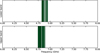 |
Fig. A.1 Waterfall plot illustrating the selected frequency channels used to construct the radio continuum images. The green-shaded regions indicate the frequency ranges included in the final continuum maps. |
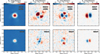 |
Fig. A.2 Stokes I, Q, U, and V maps of 3C 295 at 4.89 GHz and 6.82 GHz. The color bars are shown in units of millijansky per beam. This demonstrates a low degree of instrumental polarization. |
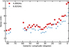 |
Fig. A.3 Total intensity noise distribution for the Effelsberg continuum surveys. |
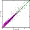 |
Fig. A.4 Comparison between the Urumqi 4.8 GHz survey and the Parkes 5 GHz survey. (a) Pixel-by-pixel comparison of the observed brightness temperatures of the two survey datasets within 10° < ℓ < 30°. The dashed red line indicates the equality between the two datasets. (b) Histogram of the brightness temperature differences between the two surveys. The vertical dashed line denotes the median value of 0.028 K. (c) Brightness temperature difference as a function of the Galactic latitude for ℓ = 11°65. The dashed red curve represents the polynomial fit to the observed distribution. |
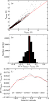 |
Fig. A.5 Pixel-by-pixel comparison of the observed brightness temperatures of the GLOSTAR and the Urumqi data within 10° < ℓ < 60°. The purple contours, derived from Gaussian kernel density estimation, represent the point density distribution. The dashed green line indicates equality between the two datasets. |
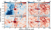 |
Fig. A.6 Zero-level restoration of the GLOSTAR 4.89 GHz polarization data in the Galactic center. Top: GLOSTAR Stokes Q and U emissions in the field within −2° < ℓ < 2°. Bottom: Corresponding Stokes Q and U images after correction using the WMAP polarization data. |
 |
Fig. A.7 Left: Observed uv coverage of the VLA D-array (blue) and its overlap with the Effelsberg data (gray ring) toward a single VLA pointing. Right: Zoom-in on the central part of the left panel. |
Appendix B Scale Height
Figure B.1 shows the mean brightness temperature as a function of Galactic latitude, averaged over the longitude range from −2° to 60°. The resulting profile is asymmetric, with a maximum at b = −0.°05. The negative latitude side appears systematically brighter than the positive side, largely due to the presence of more bright radio continuum complexes at negative latitudes (see Figs. 1 and 2). This asymmetry is also caused by the Sun’s displacement above the true Galactic midplane (e.g., Reid et al. 2019). Because the IAU coordinate system is defined relative to the Sun, objects lying in the physical midplane are observed at slightly negative latitudes. Adopting a Galactocentric distance of 8.2 kpc for the Sun (Reid et al. 2019), the observed offset of 0.°05 corresponds to a vertical displacement of ∼7.2 pc toward negative Galactic latitudes, in good agreement with previous estimates of 5.5 ± 5.8 pc (Reid et al. 2019).
To estimate the scale height, we only make use the profile with b > −0.05°. The distribution follows an exponential decay rather than a Gaussian distribution. Fitting it with an exponential function, we obtained TB = 1.06e−(b+0.05)/0.28 + 0.23 and TB = 0.49e−(b+0.05)/0.23 + 0.11 for 4.89 GHz and 6.82 GHz, respectively. Thus, the derived scale heights are 0°.28 and 0°.23, which corresponds to scale heights of 30–40 pc at an assumed distance of 8.2 kpc. This is significantly smaller than those (0°.4–0°.6) measured from HII regions (Wood & Churchwell 1989; Giveon et al. 2005). Furthermore, the negative side appears to be have larger scale heights in terms of the 1/e level which can indicates scale heights of 0°.5–0°.7. As discussed earlier, more bright radio continuum complexes contribute more to the negative side. Overall, this suggests that the diffuse radio continuum emission is more tightly confined to the Galactic mid–plane than the more vertically extended population of HII regions.
Appendix C Large-scale template for the zero-level restoration
As discussed in Sect. 2.2, we combined the Urumqi data and the corrected Parkes data into a mosaic at a common HBPW of 15′. The resulting image, shown in Fig. C.1, illustrates a smooth transition from the Urumqi data to the Parkes data, offering a template for the large-scale distribution used in the zero-level restoration of our GLOSTAR data. This template was further used to correct the zero-level offsets, and the distributions of the restored Stokes I maps are shown in Figs. 1 and 2.
 |
Fig. B.1 Mean brightness temperature profile as a function of Galactic latitude. The vertical dashed line indicates the latitude of maximum intensity. The two horizontal lines mark the 1/e levels of the peak intensities at the two bands. The dotted lines indicate the corresponding exponential fits to the profiles. |
 |
Fig. C.1 Distribution of Stokes I intensity from the Urumqi and Parkes combined data at 5 GHz. |
All Tables
All Figures
|
Fig. 1 Effelsberg 4.89 GHz Stokes I continuum map of the entire GLOSTAR survey. Zoom-in plots of each fields are available via https://gongyan2444.github.io/glostar-snr-hii.html, where the green, gray, and red circles represent the known SNRs (Green 2025), SNR candidates (Anderson et al. 2017; Dokara et al. 2021; Anderson et al. 2025), and HII regions from the WISE catalog (Anderson et al. 2014), respectively. |
| In the text | |
|
Fig. 2 Effelsberg 6.82 GHz Stokes I continuum map of the entire GLOSTAR survey. |
| In the text | |
|
Fig. 3 Comparison of the Effelsberg 4.89 GHz Stokes I continuum map with maps from the Urumqi, GB6, and Parkes surveys at similar frequencies. |
| In the text | |
|
Fig. 4 Comparison of GLOSTAR data with and without incorporating the Effelsberg data at 5.8 GHz. (a) VLA D-array only continuum image. (b) Combination of VLA D-array and Effelsberg 100 m single-dish images. |
| In the text | |
|
Fig. 5 (a) Angular power spectra of the VLA-D array, Effelsberg-100 m, and VLA-Effelsberg combined images toward the representative region near the Galactic center (see Fig. 4). The 2D Kolmogorov-like spectrum is indicated by the dashed black line for comparison. (b) Percentage of missing flux of the VLA D-array data across the Galactic plane covered by the GLOSTAR survey. The horizontal dashed red line indicates a missing flux fraction of 10%. |
| In the text | |
|
Fig. 6 Distribution of the Stokes I, Q, U, and polarization intensity maps from the Effelsberg 4.89 GHz continuum emission of the GLOSTAR survey. Zoom-in plots of each fields are available via https://gongyan2444.github.io/glostar-snr-hii.html, where the green, gray, and red circles represent the known SNRs (Green 2025), SNR candidates (Anderson et al. 2017; Dokara et al. 2021; Anderson et al. 2025), and HII regions from the WISE catalog (Anderson et al. 2014), respectively. |
| In the text | |
|
Fig. 7 Distribution of the Stokes I, Q, U, and polarization intensity maps from the Effelsberg 6.82 GHz continuum emission of the GLOSTAR survey. |
| In the text | |
|
Fig. 8 Observed properties of G016.648−00.357 (i.e., Sh 2-48). (a) Effelsberg 4.89 GHz Stokes I image overlaid with the GDIGS RRL integrated-intensity contours. (b) TT plot between 4.89 GHz and 6.82 GHz at a common angular resolution of 2′.65. The dashed red line shows the best fit to the observed data points. (c) Spatial distribution of the derived electron temperatures overlaid with the GDIGS RRL integrated-intensity contours. In panels (a) and (c), the integrated velocity ranges from 0 to 70 km s−1 for the GDIGS RRL integrated intensity contours, starting at 1 K km s−1 and increasing by 0.5 K km s−1. The location of the exciting star BD−14 5014 is marked with a gold star. In each panel, the beam is shown in the lower-left corner, and the scale bar in the top-right corner is based on an assumed distance of 3.8 kpc (e.g., Ortega et al. 2013; Torii et al. 2021). |
| In the text | |
|
Fig. 9 GLOSTAR radio continuum data of W28. (a) Linear polarization intensity maps overlaid with the magnetic-field vectors from the 2.695 GHz Effelsberg Galactic plane survey. The white contours represent the 2.695 GHz Stokes I continuum emission, starting at 2.5 K and increasing in steps of 2.5 K. (b) Similar to panel a, but using GLOSTAR 4.89 GHz continuum data, with white contours starting at 1.0 K and increasing in steps of 1.0 K. (c) Similar to panel a, but based on GLOSTAR 6.82 GHz continuum data, where white contours start at 0.5 K and increase in steps of 0.5 K. In panels a–c, the polarization angles are rotated by 90° to trace the magnetic-field directions, indicated by black bars. The position of the runaway pulsar PSR B1758−23 (i.e., PSR J1801−23), thought to be associated with W28 (Frail et al. 1993), is indicated by a cyan star. In each panel, the beam is shown in the lower-left corner, and the scale bar in the top-right corner is based on an assumed distance of 2 kpc (Velázquez et al. 2002). (d) TT plot of the northeastern shell between 4.89 GHz and 6.82 GHz at a common angular resolution of 160′′. The dashed red line shows the best fit to the observed data points extracted from the region displayed in the panel in the lower right corner. (e) Distribution of the derived RMs. |
| In the text | |
|
Fig. A.1 Waterfall plot illustrating the selected frequency channels used to construct the radio continuum images. The green-shaded regions indicate the frequency ranges included in the final continuum maps. |
| In the text | |
|
Fig. A.2 Stokes I, Q, U, and V maps of 3C 295 at 4.89 GHz and 6.82 GHz. The color bars are shown in units of millijansky per beam. This demonstrates a low degree of instrumental polarization. |
| In the text | |
|
Fig. A.3 Total intensity noise distribution for the Effelsberg continuum surveys. |
| In the text | |
|
Fig. A.4 Comparison between the Urumqi 4.8 GHz survey and the Parkes 5 GHz survey. (a) Pixel-by-pixel comparison of the observed brightness temperatures of the two survey datasets within 10° < ℓ < 30°. The dashed red line indicates the equality between the two datasets. (b) Histogram of the brightness temperature differences between the two surveys. The vertical dashed line denotes the median value of 0.028 K. (c) Brightness temperature difference as a function of the Galactic latitude for ℓ = 11°65. The dashed red curve represents the polynomial fit to the observed distribution. |
| In the text | |
|
Fig. A.5 Pixel-by-pixel comparison of the observed brightness temperatures of the GLOSTAR and the Urumqi data within 10° < ℓ < 60°. The purple contours, derived from Gaussian kernel density estimation, represent the point density distribution. The dashed green line indicates equality between the two datasets. |
| In the text | |
|
Fig. A.6 Zero-level restoration of the GLOSTAR 4.89 GHz polarization data in the Galactic center. Top: GLOSTAR Stokes Q and U emissions in the field within −2° < ℓ < 2°. Bottom: Corresponding Stokes Q and U images after correction using the WMAP polarization data. |
| In the text | |
|
Fig. A.7 Left: Observed uv coverage of the VLA D-array (blue) and its overlap with the Effelsberg data (gray ring) toward a single VLA pointing. Right: Zoom-in on the central part of the left panel. |
| In the text | |
|
Fig. B.1 Mean brightness temperature profile as a function of Galactic latitude. The vertical dashed line indicates the latitude of maximum intensity. The two horizontal lines mark the 1/e levels of the peak intensities at the two bands. The dotted lines indicate the corresponding exponential fits to the profiles. |
| In the text | |
|
Fig. C.1 Distribution of Stokes I intensity from the Urumqi and Parkes combined data at 5 GHz. |
| In the text | |
Current usage metrics show cumulative count of Article Views (full-text article views including HTML views, PDF and ePub downloads, according to the available data) and Abstracts Views on Vision4Press platform.
Data correspond to usage on the plateform after 2015. The current usage metrics is available 48-96 hours after online publication and is updated daily on week days.
Initial download of the metrics may take a while.