| Issue |
A&A
Volume 699, July 2025
|
|
|---|---|---|
| Article Number | L2 | |
| Number of page(s) | 5 | |
| Section | Letters to the Editor | |
| DOI | https://doi.org/10.1051/0004-6361/202555384 | |
| Published online | 25 June 2025 | |
Letter to the Editor
First detection of HS2 in a cold dark cloud
1
Observatorio Astronómico Nacional (OAN), Alfonso XII, 3, 28014 Madrid, Spain
2
Observatorio de Yebes, IGN, Cerro de la Palera s/n, E-19141 Yebes, Guadalajara, Spain
3
Instituto de Física Fundamental, CSIC, Calle Serrano 123, E-28006 Madrid, Spain
⋆ Corresponding authors: This email address is being protected from spambots. You need JavaScript enabled to view it.
; This email address is being protected from spambots. You need JavaScript enabled to view it.
Received:
5
May
2025
Accepted:
3
June
2025
Abstract
We report the first detection of HS2 towards the cold dark cloud TMC-1. This is the first observation of a chemical species containing more than one sulphur atom in this type of sources. The astronomical observations are part of QUIJOTE, a line survey of TMC-1 in the Q band (31–50 GHz). The detection is confirmed by the observation of the fine and hyperfine components of two rotational transitions (20, 2–10, 1 and 30, 3–20, 2). Assuming a rotational temperature of 7 K, we derived an HS2 column density of 5.7 × 1011 cm−2, using a local thermodynamic equilibrium model that reproduces the observed spectra. The abundance of HS2 relative to H2 is 5.7 × 10⁻¹¹, which means that it is about seven times more abundant than its oxygenated counterpart HSO. We also explored the main formation and destruction mechanisms of HS2 using a chemical model, which reproduces the observed abundance of HS2 and indicates that dissociative recombination reactions from the ions H2S2+ and H3S2+ play a major role in forming HS2.
Key words: ISM: abundances / ISM: clouds / ISM: molecules
© The Authors 2025
 Open Access article, published by EDP Sciences, under the terms of the Creative Commons Attribution License (https://creativecommons.org/licenses/by/4.0), which permits unrestricted use, distribution, and reproduction in any medium, provided the original work is properly cited.
This article is published in open access under the Subscribe to Open model. This email address is being protected from spambots. You need JavaScript enabled to view it. to support open access publication.
1. Introduction
Up to date, over 330 molecules have been detected1 in the interstellar medium (ISM), from which about 10% contain sulphur atoms. Ultra-sensitive spectral surveys carried out in the last few years, such as QUIJOTE (e.g. Cernicharo et al. 2021a,b) and GOTHAM (e.g. Remijan et al. 2025), have allowed the discovery of about 20% of all known sulphur species in space. Sulphur (S) is the tenth most abundant element in the Universe and is known to play a significant role in biological systems, with presence in different biomolecules (e.g. Chatterjee & Hausinger 2022). On Earth, S supports the chemoautotrophic and the photosynthetic ways of life (e.g. Clark 1981; Narayan et al. 2023). In particular, it acts as a nutrient for plants and animals, since it is a vital component of several biochemical compounds like proteins that form such amino acids, such as methionine (Townsend et al. 2004). Sulphur is also key to the synthesis of some vitamins, such as C, B1, and B8 (e.g. Raulin & Toupance 1977; Begley et al. 1999).
Although sulphur is one of the most abundant species in the Universe, S-bearing molecules are not as abundant as expected in the ISM. In the diffuse ISM, the observed gaseous sulphur accounts (e.g. Howk et al. 2006) for its total solar abundance (S/H ∼ 1.5 × 10⁻⁵; Asplund et al. 2009). However, in dense molecular clouds and star-forming regions, there is an unexpected paucity of sulphur species. In fact, to reproduce observations in hot corinos and hot cores, a significant sulphur depletion of at least one order of magnitude lower than the solar elemental sulphur abundance must be considered (Cernicharo et al. 2021a, 2024; Esplugues et al. 2022, 2023; Hily-Blant et al. 2022; Fuente et al. 2023). In particular, the sum of all the observed gas-phase sulphur abundances constitute only < 1% of the expected amount (e.g. Fuente et al. 2019) in spite of the numerous sulphur species recently detected by QUIJOTE (e.g. Cernicharo et al. 2021a,b,c; Cabezas et al. 2025). The unknown whereabouts of the remaining S in dense clouds remains an open question. Chemical models predict that, in the dense ISM, atomic S would stick on grains and be mostly hydrogenated forming H2S (Hatchell et al. 1998; Garrod et al. 2007; Esplugues et al. 2014), especially at low (< 20 K) temperatures (Druard & Wakelam 2012). However, H2S has never been detected in interstellar ices. Models and laboratory experiments also suggest that sulphur could be locked into pure S-allotropes (Sx) or into hydrogen sulphides (HxSy) (Jiménez-Escobar & Muñoz Caro 2011; Shingledecker et al. 2020). This has led to a number of observational searches for these S-species in different star-forming regions (Esplugues et al. 2013; Martín-Doménech et al. 2016) without success. Only upper limits for H2S2 and HS2 could be derived. In fact, unlike their oxygenated counterparts (H2O2, HO2, and HSO), which have been already detected (Bergman et al. 2011; Parise et al. 2012; Marcelino et al. 2023), H2S2 still remains undetected in space, and HS2 has only been detected in the Horsehead photon-dominated region (Fuente et al. 2017, 2025), thus maintaining the mystery of sulphur absence in cold regions.
In this Letter, we report the first detection of HS2 in the cold dark cloud TMC-1, providing new insights into the sulphur chemistry in star-forming regions. Observations are described in Sect. 2. We also present and discuss our results in Sects. 3 and 4, respectively, where we also include the use of chemical models to study the most plausible HS2 formation paths considering gas-phase and surface chemical reactions. We finally summarise our conclusions in Sect. 5.
2. Observations
The observations presented in this work are from the ongoing QUIJOTE line survey carried out with the Yebes 40 m telescope. A detailed description of the line survey and the data-analysis procedure are provided in Cernicharo et al. (2021d). QUIJOTE consists of a line spectral survey in the Q band (31.0–50.3 GHz) at the position of the cyanopolyyne peak of TMC-1 (αJ2000 = 04h:41m:41.9s, δJ2000 = 25o:41′:27.0″). The survey was performed in several sessions between 2019 and 2024, using new receivers built within the Nanocosmos project2 and installed at the Yebes 40 m telescope (Tercero et al. 2021). The Q band receiver consists of two cold high-electron-mobility transistor amplifiers (HEMT) that cover the 31.0–50.3 GHz band with horizontal and vertical polarisations. Fast Fourier transform spectrometers (FFTSs) with 8 × 2.5 GHz and a spectral resolution of 38.15 kHz (∼0.27 km s−1) was also used. The observational mode was frequency-switching with frequency throws of either 10 or 8 MHz. In addition, different central frequencies were used during the runs in order to check that no spurious spectral ghosts were produced in the down-conversion chain. The total observing time on the source for the data taken with the frequency throws of 10 MHz and 8 MHz is 772.6 and 736.6 hours, respectively. Hence, the total observing time on source is 1509.2 hours. The QUIJOTE sensitivity varies between 0.06 mK at 32 GHz and 0.18 mK at 49.5 GHz.
The intensity scale in antenna temperature ( , which is corrected for atmospheric absorption and for antenna ohmic and spillover losses) was calibrated using two absorbers at different temperatures and the atmospheric transmission model (ATM; Cernicharo 1985; Pardo et al. 2001). The absolute calibration uncertainty is 10%. The data were reduced and processed by using the CLASS package provided within the GILDAS software3, developed by the IRAM Institute.
3. Results
In the analysis of the 7 mm line survey of TMC-1, we detected five lines of HS2 corresponding to different hyperfine components of the rotational transitions 20, 2–10, 1 and 30, 3–20, 2 (whose energies are Eu = 2.2 and 4.5 K, respectively), using the Cologne Database for Molecular Spectroscopy (CDMS, Müller et al. 2001, 2005; Endres et al. 2016) and the MADEX code (Cernicharo 2012). This molecule shows fine and hyperfine components due to electron and nuclear spin hyperfine interactions. In particular, we detected four lines of HS2 above 4σ (20, 2–10, 1, J = 5/2 − 3/2, F = 2 − 1; 20, 2–10, 1, J = 5/2 − 3/2, F = 3 − 2; 30, 3–20, 2, J = 7/2 − 5/2, F = 4 − 3; and 30, 3–20, 2, J = 5/2 − 3/2, F = 3 − 2) and one at the 3.5σ level (20, 2–10, 1, J = 3/2 − 1/2, F = 2 − 1). The other three hyperfine transitions covered in the Q band (20, 2–10, 1, J = 3/2 − 1/2, F = 1 − 0; 30, 3–20, 2, J = 7/2 − 5/2, F = 3 − 2; and 30, 3–20, 2, J = 5/2 − 3/2, F = 2 − 1) were not detected due to their lower line strength and/or because the noise was significantly higher in that region of the spectrum. The detected lines present antenna temperatures between 0.47 and 1.44 mK, and line-widths ranging from 0.96 to 1.85 km s−1, similar to those found for other sulphur species in TMC-1 (Marcelino et al. 2023; Agúndez et al. 2025). In addition, they are not blended with any other spectral feature. Table 1 lists the line parameters obtained from Gaussian fits of the detected lines. Figure 1 shows the line profiles (black lines) of HS2 for the transitions 20, 2–10, 1 and 30, 3–20, 2.
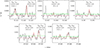 |
Fig. 1. Observed lines of HS2 in TMC-1 in the 31.0–50.4 GHz range. Quantum numbers are indicated in each panel. The red line shows the LTE synthetic spectrum from a fit to the observed line profiles. The negative features are created in the folding of the frequency switching data. The horizontal green line indicates the 3σ noise level. |
In order to calculate the column density of HS2, we used the MADEX code assuming local thermodynamic equilibrium (LTE) due to the lack of collisional rates. An LTE approximation means that most transitions are thermalised to the same temperature (Trot ∼ TK). If this condition is not met, the temperature might be overestimated, which would produce a variation in the column density. In our case, we used a Trot from the transition analysis and find that the considered value is in good agreement with the one obtained for other sulphur molecules in the same region (see below). Nevertheless, it should also be considered that, since the upper energy levels are very low (2.2 and 4.5 K, Table 1), the column density is not very sensitive as long as Trot is equal to or higher than 4.5 K.
Line parameters obtained from Gaussian fits of the detected HS2 lines in TMC-1.
The MADEX code takes the different telescope beams and efficiencies into account to obtain antenna temperature intensities for each line. We assumed a diameter size of 80″ (Fossé et al. 2001), compatible with the emission size of most of the molecules mapped in TMC-1 (Cernicharo et al. 2023). We also considered a line-width of 1.3 km s−1 from the average value obtained from the Gaussian fits to the HS2 lines (Table 1). We left the rotational temperature and the column density as free parameters. Taken together, the model that best reproduces the line profiles of HS2 is the one with a rotational temperature of 7 K, in good agreement with the results from Marcelino et al. (2023) and Agúndez et al. (2025) for the analysis of HSO and CH3CHS, respectively. Figure 1 shows the synthetic spectra from the LTE models in red, overlaid with the observed line profiles (black). We derive an HS2 column density of (5.7 ± 1.1) × 1011 cm−2. The error in the column density is estimated to be 20%. Adopting an H2 column density of 1022 cm−2 for TMC-1 (Cernicharo & Guelin 1987), we obtain an HS2 abundance relative to H2 of (5.7 ± 1.1) × 10−11, which is similar to that obtained by Fuente et al. (2017) in the Horsehead PDR.
4. Discussion
The low temperatures obtained from the LTE models indicate that HS2 emission arises from the cold envelope of TMC-1. Low temperatures have also been observed in TMC-1 for other such sulphur specie as SO (∼4 K, Loison et al. 2019) and HSO (∼4.5 K, Marcelino et al. 2023), which suggests a common origin. Particularly interesting is the comparison between HS2 and its oxygenated counterparts HO2 and HSO since sulphur belongs to the chalcogens, along with oxygen. Their similar electron configuration could indicate a similar chemistry; nevertheless, their abundances are quite different. In particular, the abundance of HSO relative to H2 is 7 × 10⁻¹² (Marcelino et al. 2023) is almost one order of magnitude lower than that of HS2 in TMC-1. This trend of low HSO abundance with respect to HS2 is maintained throughout the time evolution of the cloud, according to the chemical model shown in Fig. B.1 (Appendix B), which was obtained using the public Nautilus chemical code4. Nautilus is a three-phase model (gas, grain surface, and grain mantle, Ruaud et al. 2016) (see Appendix A for more details). Figure B.1 also shows the time evolution of the fractional abundances for H2S, S2, and HO2, which has been detected only in ρ Ophiuchi A with an abundance of ∼10−10 (Parise et al. 2012). In Fig. B.1, H2S and HO2 have the highest and lowest abundances for t > 103 yr, respectively, with differences among them of several orders of magnitude. We also observe that HO2 and HSO follow a similar trend along the entire cloud evolution.
4.1. HS2 formation and destruction
Despite the numerous observations, laboratory experiments, and chemical modelling studies performed (e.g., Hatchell et al. 1998; Ruffle et al. 1999; Wakelam & Herbst 2008; Vidal et al. 2017; Esplugues et al. 2023), sulphur chemistry in the ISM, especially in dark clouds, is one of the least understood. All of these effotts have tried to shed light on the so-called sulphur depletion problem; however, results have been unsuccessful in predicting fractional abundances of species, such as CS, falling short by up to two orders of magnitude compared to astronomical observations. Chemical models also predict that, in the dense ISM, atomic sulphur would stick on grains and be mostly hydrogenated, or be locked into solid species, such as H2S2, CS2, and S8 (Palumbo et al. 1997; Shingledecker et al. 2020; Cazaux et al. 2022). However, the lack of observations of these species makes understanding sulphur chemistry difficult. In this way, the detection of new sulphur species in dark clouds, as well as the study of their formation mechanisms, is significantly valued.
In this regard, we carried out chemical modelling calculations using the Nautilus code to study the main formation and destruction paths of HS2. Figure B.2 (Appendix B) shows the chemical rates for the most dominant reactions forming and destroying HS2. In order to evaluate the density effect on the chemical rates, two different models were considered: one model with a cloud density of nH = 104 cm−3 (solid lines) and another model with nH = 105 cm−3 (dashed lines). We observe that the effect of varying the cloud density mainly affects the chemical rates at early evolutionary times (t ≲ 105 yr), with differences of several orders of magnitude between both models. Nonetheless, we note that these differences become smaller as the cloud evolves.
We find that HS2 is mainly formed through the dissociative recombination of the ions H3S and H2S
 , following
 (1)
(1)
 (2)
(2)
which are mainly formed in turn from the reactions:
 (3)
(3)
 (4)
(4)
respectively. In particular, we find that reaction 1 is the dominant reaction forming HS2 during t ≲ 105 yr, and that for longer times reaction 2 also becomes important. By contrast, we do not find any significant contribution from the surface reactions in the formation of HS2. Nevertheless, we should notice that some relevant surface reactions for HS2, such as
 (5)
(5)
are not included in the chemical network. While other reactions, such as
 (6)
(6)
are considered as barrierless reactions. This significantly reduces the S2 abundance on the grains and, consequently, partially deactivates that chemistry. All this highlights the poor knowledge we currently have on HS2 chemistry on grain surfaces.
Regarding its destruction, Figure B.2 shows that HS2 is mainly destroyed at early times (t < 104 yr) by
 (7)
(7)
while for a more evolved cloud (104 ≲ t ≲ 106 yr), the ions H , HCO+, and H3O+ play an important role in destroying HS2. In any case, there are also many reactions between HS2 and neutral atoms, such as H, C, or O, which are neither included in the network nor studied in detail, and which could significantly alter the theoretical HS2 abundances obtained in the models. In fact, only a few analyses on the chemistry of HS2 (only at high temperatures) are found in the literature (e.g., Sendt et al. 2002).
4.2. Model vs. observations
In order to theoretically reproduce the HS2 abundance obtained in TMC-1, and evaluate the influence of the physical parameters on HS2, we ran several models (Table B.1, Appendix B) varying density, temperature, and initial sulphur abundance. All the models were run considering AV = 15 mag, which was derived from visual extinction maps from Herschel data (Navarro-Almaida et al. 2021), and a cosmic-ray ionisation rate of ζ = 1.3 × 10⁻¹⁷ s−1, according to the value derived by Navarro-Almaida et al. (2021) in TMC-1 by comparing spectroscopic observations with theoretical results. Figure B.3 (Appendix B) shows our results. We find that the observations are reproduced by all the models considering an initial sulphur abundance of 1.5 × 10⁻⁶. In general, we observe that the more depleted the sulphur is, the lower the HS2 abundance throughout the cloud’s evolution. In particular, decreasing the initial sulphur abundance by one order of magnitude leads to a decrease in HS2 abundance by about 2–3 orders of magnitude. The density also has a key role in HS2 abundance, especially at t < 105 yr, where we find that increasing nH by one order of magnitude leads to significantly higher abundances of HS2 owing to the higher collision rates of reactions 1–4.
In any case, our models reproduce the observations of HS2 when  × 10−6, for an evolutionary time of t ≳ 104 yr if the cloud density is nH = 104 cm−3, or at t > 103 yr if nH = 105 cm−3.
5. Conclusions
We report the first detection of HS2 in a cold dark cloud (TMC-1), thanks to the highly sensitive QUIJOTE Q-band spectral line survey. This is the first observation of a chemical species containing more than one sulphur atom in this type of source. Our analysis reveals that its molecular emission arises from the very cold envelope of TMC-1, with an abundance similar to that found in the Horsehead PDR, but almost one order of magnitude higher than that for its oxygenated counterpart HSO in TMC-1. A chemical analysis also shows that gas-phase chemical reactions, in particular dissociative recombination reactions, play a major role forming HS2. This molecules is very sensitive to the cloud density and to the sulphur depletion degree.
Acknowledgments
This work was based on observations carried out with the Yebes 40m telescope (projects 19A003, 20A014, 20D023, 21A011, 21D005, and 23A024). Yebes 40 m telescope is operated by the Spanish Geographic Institute (IGN, Ministerio de Transportes y Movilidad Sostenible). We acknowledge funding support from Spanish Ministerio de Ciencia e Innovación through grants PID2022-137980NB-I00, PID2022-136525NA-I00 and PID2023-147545NB-I00. G. E. acknowledges sthe ERC project SUL4LIFE (grant agreement No101096293) from European Union. G. M. acknowledges the support of the grant RYC2022-035442-I funded by MICIU/AEI/10.13039/501100011033 and ESF+. G. M. also received support from project 20245AT016 (Proyectos Intramurales CSIC). We also thank the anonymous referee for valuable comments that improved the manuscript.
References
- Agúndez, M., Molpeceres, G., Cabezas, C., et al. 2025, A&A, 693, L20 [NASA ADS] [CrossRef] [EDP Sciences] [Google Scholar]
- Asplund, M., Grevesse, N., Sauval, A. J., & Scott, P. 2009, ARA&A, 47, 481 [NASA ADS] [CrossRef] [Google Scholar]
- Begley, T. P., Xi, J., Kinsland, C., Taylor, S., & McLafferty, F. 1999, Chem. Biol., Elsevier Sci., 3, 623 [Google Scholar]
- Bergman, P., Parise, B., Liseau, R., et al. 2011, A&A, 531, L8 [NASA ADS] [CrossRef] [EDP Sciences] [Google Scholar]
- Cabezas, C., Vávra, K., Molpeceres, G., et al. 2025, A&A, 698, L24 [NASA ADS] [CrossRef] [EDP Sciences] [Google Scholar]
- Cazaux, S., Carrascosa, H., Muñoz Caro, G. M., et al. 2022, A&A, 657, A100 [NASA ADS] [CrossRef] [EDP Sciences] [Google Scholar]
- Cernicharo, J. 1985, Internal IRAM report (Granada: IRAM) [Google Scholar]
- Cernicharo, J. 2012, EAS Publ. Ser., 58, 251 [Google Scholar]
- Cernicharo, J., & Guelin, M. 1987, A&A, 176, 299 [NASA ADS] [Google Scholar]
- Cernicharo, J., Cabezas, C., Agúndez, M., et al. 2021a, A&A, 648, L3 [EDP Sciences] [Google Scholar]
- Cernicharo, J., Cabezas, C., Endo, Y., et al. 2021b, A&A, 650, L14 [NASA ADS] [CrossRef] [EDP Sciences] [Google Scholar]
- Cernicharo, J., Cabezas, C., Endo, Y., et al. 2021c, A&A, 646, L3 [EDP Sciences] [Google Scholar]
- Cernicharo, J., Agúndez, M., Kaiser, R. I., et al. 2021d, A&A, 652, L9 [NASA ADS] [CrossRef] [EDP Sciences] [Google Scholar]
- Cernicharo, J., Tercero, B., Marcelino, N., Agúndez, M., & de Vicente, P. 2023, A&A, 674, L4 [NASA ADS] [CrossRef] [EDP Sciences] [Google Scholar]
- Cernicharo, J., Cabezas, C., Agúndez, M., et al. 2024, A&A, 688, L13 [NASA ADS] [CrossRef] [EDP Sciences] [Google Scholar]
- Chatterjee, S., & Hausinger, R. P. 2022, Crit. Rev. Biochem. Mol. Biol., 57, 461 [Google Scholar]
- Clark, B. C. 1981, in NASA Conference Publication, ed. J. Billingham, 2156, 47 [Google Scholar]
- Druard, C., & Wakelam, V. 2012, MNRAS, 426, 354 [NASA ADS] [CrossRef] [Google Scholar]
- Endres, C. P., Schlemmer, S., Schilke, P., Stutzki, J., & Müller, H. S. P. 2016, J. Mol. Spectrosc., 327, 95 [NASA ADS] [CrossRef] [Google Scholar]
- Esplugues, G. B., Tercero, B., Cernicharo, J., et al. 2013, A&A, 556, A143 [NASA ADS] [CrossRef] [EDP Sciences] [Google Scholar]
- Esplugues, G. B., Viti, S., Goicoechea, J. R., & Cernicharo, J. 2014, A&A, 567, A95 [NASA ADS] [CrossRef] [EDP Sciences] [Google Scholar]
- Esplugues, G., Fuente, A., Navarro-Almaida, D., et al. 2022, A&A, 662, A52 [NASA ADS] [CrossRef] [EDP Sciences] [Google Scholar]
- Esplugues, G., Rodríguez-Baras, M., San Andrés, D., et al. 2023, A&A, 678, A199 [NASA ADS] [CrossRef] [EDP Sciences] [Google Scholar]
- Fossé, D., Cernicharo, J., Gerin, M., & Cox, P. 2001, ApJ, 552, 168 [Google Scholar]
- Fuente, A., Goicoechea, J. R., Pety, J., et al. 2017, ApJ, 851, L49 [NASA ADS] [CrossRef] [Google Scholar]
- Fuente, A., Navarro, D. G., Caselli, P., et al. 2019, A&A, 624, A105 [NASA ADS] [CrossRef] [EDP Sciences] [Google Scholar]
- Fuente, A., Rivière-Marichalar, P., Beitia-Antero, L., et al. 2023, A&A, 670, A114 [NASA ADS] [CrossRef] [EDP Sciences] [Google Scholar]
- Fuente, A., Esplugues, G., Rivière-Marichalar, P., et al. 2025, ApJ, 986, L17 [Google Scholar]
- Garrod, R. T., Wakelam, V., & Herbst, E. 2007, A&A, 467, 1103 [NASA ADS] [CrossRef] [EDP Sciences] [Google Scholar]
- Graedel, T. E., Langer, W. D., & Frerking, M. A. 1982, ApJS, 48, 321 [NASA ADS] [CrossRef] [Google Scholar]
- Hatchell, J., Thompson, M. A., Millar, T. J., & MacDonald, G. H. 1998, A&AS, 133, 29 [NASA ADS] [CrossRef] [EDP Sciences] [Google Scholar]
- Hily-Blant, P., Pineau des Forêts, G., Faure, A., & Lique, F. 2022, A&A, 658, A168 [NASA ADS] [CrossRef] [EDP Sciences] [Google Scholar]
- Howk, J. C., Sembach, K. R., & Savage, B. D. 2006, ApJ, 637, 333 [NASA ADS] [CrossRef] [Google Scholar]
- Jiménez-Escobar, A., & Muñoz Caro, G. M. 2011, A&A, 536, A91 [Google Scholar]
- Jiménez-Serra, I., Viti, S., Quénard, D., & Holdship, J. 2018, ApJ, 862, 128 [CrossRef] [Google Scholar]
- Loison, J.-C., Wakelam, V., Gratier, P., et al. 2019, MNRAS, 485, 5777 [Google Scholar]
- Marcelino, N., Puzzarini, C., Agúndez, M., et al. 2023, A&A, 674, L13 [NASA ADS] [CrossRef] [EDP Sciences] [Google Scholar]
- Martín-Doménech, R., Jiménez-Serra, I., Muñoz Caro, G. M., et al. 2016, A&A, 585, A112 [NASA ADS] [CrossRef] [EDP Sciences] [Google Scholar]
- Morton, D. C. 1974, ApJ, 193, L35 [NASA ADS] [CrossRef] [Google Scholar]
- Müller, H. S. P., Thorwirth, S., Roth, D. A., & Winnewisser, G. 2001, A&A, 370, L49 [Google Scholar]
- Müller, H. S. P., Schlöder, F., Stutzki, J., & Winnewisser, G. 2005, J. Mol. Struct., 742, 215 [Google Scholar]
- Narayan, O. P., Kumar, P., Yadav, B., & Joohri, A. K. 2023, Plant Signaling Behav., 18, 1 [Google Scholar]
- Navarro-Almaida, D., Fuente, A., Majumdar, L., et al. 2021, A&A, 653, A15 [NASA ADS] [CrossRef] [EDP Sciences] [Google Scholar]
- Neufeld, D. A., Wolfire, M. G., & Schilke, P. 2005, ApJ, 628, 260 [Google Scholar]
- Palumbo, M. E., Geballe, T. R., & Tielens, A. G. G. M. 1997, ApJ, 479, 839 [NASA ADS] [CrossRef] [Google Scholar]
- Pardo, J. R., Cernicharo, J., & Serabyn, E. 2001, IEEE Trans. Antennas Propag., 49, 1683 [Google Scholar]
- Parise, B., Bergman, P., & Du, F. 2012, A&A, 541, L11 [NASA ADS] [CrossRef] [EDP Sciences] [Google Scholar]
- Prasad, S. S., & Tarafdar, S. P. 1983, ApJ, 267, 603 [Google Scholar]
- Raulin, F., & Toupance, G. 1977, J. Mol. Evol., 9, 329 [Google Scholar]
- Remijan, A. J., Changala, P. B., Xue, C., et al. 2025, ApJ, 982, 191 [Google Scholar]
- Ruaud, M., Wakelam, V., & Hersant, F. 2016, MNRAS, 459, 3756 [Google Scholar]
- Ruffle, D. P., Hartquist, T. W., Caselli, P., & Williams, D. A. 1999, MNRAS, 306, 691 [Google Scholar]
- Sendt, K., Jazbec, M., & Haynes, B. S. 2002, Elsevier, 29, 2439 [Google Scholar]
- Shingledecker, C. N., Lamberts, T., Laas, J. C., et al. 2020, ApJ, 888, 52 [Google Scholar]
- Tercero, F., López-Pérez, J. A., Gallego, J. D., et al. 2021, A&A, 645, A37 [EDP Sciences] [Google Scholar]
- Townsend, D. M., Tew, K. D., & Tapiero, H. 2004, Biomedicine and Pharmacotherapy, 58, 47 [Google Scholar]
- Vidal, T. H. G., Loison, J.-C., Jaziri, A. Y., et al. 2017, MNRAS, 469, 435 [Google Scholar]
- Wakelam, V., & Herbst, E. 2008, ApJ, 680, 371 [NASA ADS] [CrossRef] [Google Scholar]
- Wakelam, V., Dartois, E., Chabot, M., et al. 2021, A&A, 652, A63 [NASA ADS] [CrossRef] [EDP Sciences] [Google Scholar]
- Wakelam, V., Gratier, P., Loison, J. C., et al. 2024, A&A, 689, A63 [NASA ADS] [CrossRef] [EDP Sciences] [Google Scholar]
Appendix A: Nautilus chemical code
The Nautilus chemical code (Ruaud et al. 2016) solves the kinetic equations for both the gas phase species and the grain surface species, and computes the time evolution of chemical abundances. Gas-phase chemical reactions included in Nautilus are bimolecular reactions (neutral-neutral and ion-neutral reactions), direct cosmic-ray ionisation or dissociation, ionisation and dissociation by UV photons, ionisation and dissociation produced by photons induced by cosmic-ray interactions with the medium (Prasad & Tarafdar 1983), and electron recombinations. Regarding chemical grain surface processes, the code includes sputtering of grains by cosmic ray particles (CR sputtering), and non-thermal desorption (distinguishing between three types of desorption: photo-desorption, chemical desorption, and cosmic-ray heating). These three types of desorption are only allowed to occur for surface species, while CR sputtering can take place for both surface and mantle species. The chemical network used in Nautilus is based on the KInetic Database for Astrochemistry (KIDA5). In particular, it is the chemical network kida.uva.2022, which contains the updates presented in Wakelam et al. (2024) and new non-thermal desorption mechanisms, such as cosmic-ray sputtering, as described in Wakelam et al. (2021). Nautilus is run considering the initial abundances shown in Table A.1.
Abundances with respect to total hydrogen nuclei considered in the chemical code Nautilus.
Appendix B: Tables and Figures
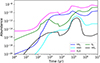 |
Fig. B.1. Evolution of fractional abundances (nx/nH) of HS2 (blue), HSO (cyan), H2S (magenta), S2 (green), and HO2 (black) as a function of time for an initial sulphur abundance of |

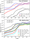 |
Fig. B.2. Main chemical reaction rates forming (top) and destroying (bottom) HS2. JX means solid X. |
Adopted model parameters.
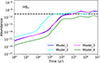 |
Fig. B.3. Comparison of the observational HS2 abundance in TMC-1 with the fractional abundances obtained with Models 1-4. Dashed black line represents the observed HS2 abundance. |
All Tables
Abundances with respect to total hydrogen nuclei considered in the chemical code Nautilus.
All Figures
|
Fig. 1. Observed lines of HS2 in TMC-1 in the 31.0–50.4 GHz range. Quantum numbers are indicated in each panel. The red line shows the LTE synthetic spectrum from a fit to the observed line profiles. The negative features are created in the folding of the frequency switching data. The horizontal green line indicates the 3σ noise level. |
| In the text | |
|
Fig. B.1. Evolution of fractional abundances (nx/nH) of HS2 (blue), HSO (cyan), H2S (magenta), S2 (green), and HO2 (black) as a function of time for an initial sulphur abundance of |
| In the text | |
|
Fig. B.2. Main chemical reaction rates forming (top) and destroying (bottom) HS2. JX means solid X. |
| In the text | |
|
Fig. B.3. Comparison of the observational HS2 abundance in TMC-1 with the fractional abundances obtained with Models 1-4. Dashed black line represents the observed HS2 abundance. |
| In the text | |
Current usage metrics show cumulative count of Article Views (full-text article views including HTML views, PDF and ePub downloads, according to the available data) and Abstracts Views on Vision4Press platform.
Data correspond to usage on the plateform after 2015. The current usage metrics is available 48-96 hours after online publication and is updated daily on week days.
Initial download of the metrics may take a while.