| Issue |
A&A
Volume 699, July 2025
|
|
|---|---|---|
| Article Number | A215 | |
| Number of page(s) | 13 | |
| Section | Cosmology (including clusters of galaxies) | |
| DOI | https://doi.org/10.1051/0004-6361/202554593 | |
| Published online | 11 July 2025 | |
Central galaxy alignments
Dependence on the mass and the large-scale environment
1
CONICET, Instituto de Astronomía Teórica y Experimental (IATE), Laprida 854, Córdoba X5000BGR, Argentina
2
Universidad Nacional de Córdoba (UNC), Observatorio Astronómico de Córdoba (OAC), Laprida 854, Córdoba X5000BGR, Argentina
3
Kavli IPMU (WPI), UTIAS, The University of Tokyo, Kashiwa, Chiba 277-8583, Japan
4
Max Planck Institute for Astrophysics, Karl-Schwarzschild-Straße 1, D-85748 Garching, Germany
5
Departamento de Física, Universidad Técnica Federico Santa María, Avenida Vicuña Mackenna 3939, San Joaquín, Santiago, Chile
6
Universidad Andres Bello, Facultad de Ciencias Exactas, Departamento de Ciencias Físicas, Instituto de Astrofísica, Av. Fernández Concha 700, Santiago, Chile
⋆ Corresponding author: This email address is being protected from spambots. You need JavaScript enabled to view it.
Received:
17
March
2025
Accepted:
10
June
2025
Abstract
Context. Observations indicate that central galaxies’ main shape axes are significantly aligned with other galaxies in their group, as well as with the large-scale structure of the Universe. Simulations have corroborated this finding, providing further insights into how the shape of the stellar component aligns with the surrounding dark matter halo. Recent studies have also investigated the evolution of this alignment in bright central galaxies, revealing that the shapes of the dark matter halo and the stellar component can differ. These results suggest that assembly and merger processes have played a crucial role in the evolution of this alignment.
Aims. In this work, we aim to gain a deeper understanding of galaxy alignments by quantifying how this property is related to the mass of the halos hosting central galaxies and to the large-scale environment measured at different scales.
Methods. By studying different angles, we describe how the alignments of central galaxies depend on the masses of the halos they inhabit. We explore how the main axes of central galaxies align across different scales, both in three-dimensional and two-dimensional projections. We examine how halo mass influences these alignments and how they vary in the surrounding large-scale environment. Additionally, we analyse the characteristics of these alignments across different environments within the large-scale structure of the Universe. To conduct this study, we employed TNG300 hydrodynamical simulations and compared our results with spectroscopic data from the Sloan Digital Sky Survey Data Release 18 (SDSS DR18).
Results. Three types of alignment were analysed: between stellar and dark matter components, between satellite galaxies and the central galaxy, and between the central galaxy and its host halo. The results show that the alignment increases with halo mass and varies with the environment (cluster, filament, cluster outskirt, and others). However, after controlling for local density, we found that most of the observed trends disappear, except for a marginal influence of cosmic filaments on some of the considered alignment angles. The SDSS observations confirm a mass dependence similar to the simulations, although observational biases limit the detection of differences between the different environments.
Key words: methods: statistical / galaxies: groups: general / galaxies: halos / dark matter / large-scale structure of Universe
© The Authors 2025
 Open Access article, published by EDP Sciences, under the terms of the Creative Commons Attribution License (https://creativecommons.org/licenses/by/4.0), which permits unrestricted use, distribution, and reproduction in any medium, provided the original work is properly cited.
This article is published in open access under the Subscribe to Open model. This email address is being protected from spambots. You need JavaScript enabled to view it. to support open access publication.
1. Introduction
Galaxies form and evolve within a large-scale structure predominantly made up of dark matter (DM). Their spatial distribution is influenced by gravitational forces acting initially on tiny fluctuations in the early Universe. As structures develop hierarchically through gravitational instability, the tidal fields, the process of matter accretion, and even baryonic physics are expected to subtly affect the properties of galaxies and DM halos. In this scenario, galaxies will tend to have preferred shapes, orientations, and distributions depending on the halo in which they form and, potentially, the surrounding local and large-scale environment.
Several observational works have investigated these so-called intrinsic alignments, which are expected to have important implications for the extraction of cosmological information from upcoming galaxy surveys (e.g. Hirata et al. 2007; Troxel & Ishak 2015; Joachimi et al. 2015; Kirk et al. 2015). Evidence suggests that the alignment of galaxies with each other and with large-scale cosmic structures is influenced not only by their luminosity, colour, and star formation history, but also their position within the host halo and cosmic environment. In this context, red or elliptical galaxies in general tend to display more significant alignments on a variety of scales (see e.g. Sales & Lambas 2004; Yang et al. 2006; Agustsson & Brainerd 2010; Kirk et al. 2015; Rodriguez et al. 2022; Smith et al. 2023; Desai & Ryden 2022). Moreover, red satellite galaxies show a stronger preference to align with the galactic plane of red central galaxies (Yang et al. 2005; Wang et al. 2008; Kiessling et al. 2015; Kirk et al. 2015; Libeskind et al. 2015; Welker et al. 2018; Pawlowski 2018; Johnston et al. 2019). This specific connection between star formation activity, or lack thereof, and galaxy alignments is sometimes referred to as anisotropic quenching or angular conformity (Wang et al. 2008; Stott 2022; Ando et al. 2023), an obvious reference to the correlation effect called galactic conformity (see Bray et al. 2016; Otter et al. 2020; Maier et al. 2022; Lacerna et al. 2022, and references therein).
The shape of spiral galaxies, on the other hand, is usually linked to their angular momentum, which has been proposed to arise from torques produced by the external gravitational field (Heavens et al. 2000; Catelan et al. 2001; Codis et al. 2015), and tends to align parallel to filaments, in contrast to the angular momentum of higher-mass galaxies, which is preferentially perpendicular (Welker et al. 2020; Barsanti et al. 2022; Kraljic et al. 2021, and e.g. Ganeshaiah Veena et al. 2019, 2021 for studies in simulations). Despite this connection, there is little observational evidence of shape alignments in spiral galaxies (Zjupa et al. 2022; Johnston et al. 2019; Samuroff et al. 2023). However, some studies based on observations and simulations indicate that central disc galaxies show greater misalignment with their host halos, and that this misalignment decreases with an increasing halo mass and ex situ stellar mass fraction (Xu et al. 2023a, b).
In this context, a useful tool to assess the degree of alignment of a galaxy or group population with respect to any reference system is the anisotropic correlation function, which is used to compare the clustering of different sub-regions with respect to a given orientation axis (Paz et al. 2008, 2011). Rodriguez et al. (2022) applied this method to the spectroscopic data provided by Sloan Digital Sky Survey Data Release 16 (SDSS DR16; Ahumada et al. 2020), in combination with a group identification scheme (Rodriguez & Merchán 2020), to show that bright central galaxies align with both the satellites inhabiting the same halo and the nearby large-scale cosmic structures up to a distance of ≳10 Mpc. They also report a significant dependence on colour, with red central galaxies being more aligned with their environments than blue ones. A physical interpretation of these observational constraints was subsequently provided in Rodriguez et al. (2023) based on a detailed study using the IllustrisTNG1 (hereafter simply TNG) hydrodynamical simulation. The intrinsic alignments of Rodriguez et al. (2023) are decomposed in a series of correlations and sub-dependences across scales, whereby the alignment between the baryonic component of the central galaxy and the large-scale structure is mediated by internal alignments with the sub-halo and the host halo.
The results of Rodriguez et al. (2022, 2023) prompted the additional analysis of Rodriguez et al. (2024), in which the evolution of the intrinsic alignments was investigated for red and blue galaxies separately, in connection with their different assembly and merger histories. Mergers are in fact shown to be a major contributor to the build-up of these alignments for red central galaxies, as opposed to blue central galaxies, which are younger, experience fewer mergers, and have only recently acquired their oblate shape. This aligns with findings from other cosmological simulations, such as the ones in Lagos et al. (2018), based on the EAGLE simulations, which demonstrate the broader prevalence of merger-induced alignment effects. The work of Rodriguez et al. (2024) emphasises even more the multi-scale nature of the intrinsic alignments. Mergers tend to increase the alignment between the stellar content of central galaxies and their dark-matter halos, whereas the preferred orientation of halos with respect to the large-scale environment is initially stronger and tends to diminish with time.
In this work, we use both observational data from the SDSS and simulation data from TNG to investigate in greater detail the dependence of central galaxy alignments on the environment. Our analysis follows two approaches. First, we examine the dependence on stellar and halo mass, which are known to be first-order proxies for local and large-scale environments. Second, we study how alignments vary with the location of galaxies within the cosmic web. The different components of the cosmic web are identified using the Discrete Persistent Structures Extractor (DisPerSE; Sousbie 2011; Sousbie et al. 2011), a structure finder that detects critical points of the density field (maxima, minima and saddle points). By combining the DisPerSE output with a group catalogue, galaxies can be classified into specific cosmic environments, such as filaments, clusters, or cluster outskirts. This analysis complements several other works in which DisPerSE has been employed to investigate the link between the properties of galaxies and halos and the cosmic web, including the dependence of gas accretion and star formation in galaxies (Galárraga-Espinosa et al. 2023), galaxy clustering and assembly bias (Montero-Dorta & Rodriguez 2024), halo occupation distributions (Perez et al. 2024a, b), or occupancy variations (Wang et al. 2024), to name but a few.
The paper is organised as follows. Section 2 describes the simulation (TNG) and observational (SDSS) data employed in this work, along with the identification of cosmic-web environments in both datasets based on DisPerSE. The different alignments measured in this work are defined in Sect. 3. The dependence of the alignments on both mass and the cosmic-web environment as measured from TNG is presented in Sects. 4 and 5, respectively. Section 6 focuses on the measurements performed on the SDSS, including a comparison with the simulation-based results. Finally, Sect. 7 summarises the main conclusions of our work, while discussing their implications and potential ramifications. The TNG simulation adopts the standard ΛCDM cosmology (Planck Collaboration XIII 2016), with parameters Ωm = 0.3089, Ωb = 0.0486, ΩΛ = 0.6911, H0 = 100 h km s−1 Mpc−1 with h = 0.6774, σ8 = 0.8159, and ns = 0.9667.
2. Data
2.1. The TNG hydrodynamical simulation
In this study, we utilise the galaxy and dark-matter halo catalogues from the Illustris TNG300 simulation at (z = 0, referred to as TNG300, Nelson et al. 2019; Pillepich et al. 2018a). The TNG magneto-hydrodynamical cosmological simulations were executed using the arepo moving-mesh code (Springel 2010) and represent an enhanced iteration of the original Illustris simulations (Vogelsberger et al. 2014a, b; Genel et al. 2014). These simulations incorporate sub-grid models that address factors such as radiative metal-line gas cooling, star formation, chemical enrichment from SNII, SNIa, and AGB stars, as well as stellar feedback processes, the formation of supermassive black holes with multi-mode quasar activity, and kinetic feedback from black holes. They adopt a cubic box with a side length of 205 h−1 Mpc and were run with 25003 dark-matter particles, each with a mass of 4.0×10⁷ h−1 M⊙. The initial conditions include 25003 gas cells, with each gas cell having a mass of 7.6×10⁶ h−1 M⊙.
A friends-of-friends (FoF) algorithm was employed to identify DM halos – referred to as groups in this paper – using a linking length of 0.2 times the mean inter-particle separation (Davis et al. 1985). The gravitationally bound substructures, hereafter referred to as sub-halos, were identified using the SUBFIND algorithm (Springel et al. 2001; Dolag et al. 2009). We define the stellar mass of galaxies, denoted as M*, as the total mass of all stellar particles associated with each sub-halo. In our analysis, following the selection criteria used in many previous works that take simulation resolution into account (e.g. Pillepich et al. 2018b; Rodriguez et al. 2023, 2024; Perez et al. 2024a), we consider all simulated galaxies with stellar mass (M★) greater than 108.5 M⊙, resulting in a total number of 429 982 galaxies. In this study, we analyse central galaxies identified as those sub-halos whose index matches the GroupFirstSub entry of their corresponding FoF group in the TNG300 simulation, selecting those with Mr<−19.5 in the r band. This yields a final sample of 89 534 systems, each containing more than 880 DM particles and 100 stellar particles. The magnitude threshold matches the group-definition criterion from Rodriguez & Merchán (2020), whereby groups must contain at least one galaxy brighter than Mr=−19.5 (defining the faintest observable centrals in optical surveys).
2.2. SDSS
To verify the consistency of the simulation results with the ones observed in large survey detections, we utilised the main galaxy sample from the SDSS Data Release 18 (DR18; Almeida et al. 2023). This release covers an extensive sky area exceeding 10 000 square degrees across five optical bandpasses (u,g,r,i,z) and includes more than 1.2 million galaxies with spectroscopic redshift data, reaching an approximate redshift of (z≃0.3). The spectroscopic version of this survey is statistically complete up to an apparent magnitude limit in the r band of 17.77, which guarantees a robust sample suitable for the analysis of large-scale structures. Each galaxy provides a wealth of information, including its positions, magnitudes, ellipticity, and the position angle of its major axis; the latter two parameters are crucial for the alignment analyses we intend to conduct. These parameters are derived from models based on either Vaucouleurs or exponential profiles. We have checked that regardless of the model used, the results presented in this work remain consistent. Therefore, following previous studies, this paper will present only the results obtained from the exponential model, pointing out that the figures would be nearly identical if the Vaucouleurs model were used instead.
To identify galaxy groups in the SDSS DR18, we followed the procedure described by Rodriguez & Merchán (2020). This algorithm combines the FoF method (Merchán & Zandivarez 2005) and halo-based techniques (Yang et al. 2005). The algorithm begins by detecting gravitationally bound systems through a percolation method adapted from Huchra & Geller (1982). Each group is assumed to contain at least one bright central galaxy, and its initial properties are estimated based on the total luminosity of its members. In the subsequent iterative step, the halo-based approach refines group memberships and recalculates halo properties on the basis of updated luminosity estimates. This process continues until convergence is reached, ensuring a reliable identification of systems across a broad range of group sizes, from small associations to rich clusters. The resulting group catalogue provides essential properties, including galaxy membership, spatial positions, and halo mass estimations (Mgroup), derived using an abundance matching technique (Vale & Ostriker 2004; Kravtsov et al. 2004; Conroy et al. 2006; Behroozi et al. 2010). This method assumes a one-to-one relationship between a group’s characteristic luminosity and its dark-matter halo mass. Additionally, galaxies within each group are classified as central and satellites, with the brightest galaxy designated as the central galaxy, while the remaining members are considered satellites (Rodriguez et al. 2021). This catalogue demonstrates strong consistency with weak gravitational lensing mass estimates (Gonzalez et al. 2021) and effectively reproduces the observed central-satellite galaxy population properties seen in numerical simulations, focusing primarily on the variations in halo occupancy distribution and the properties of member galaxies in different environments (e.g. Alfaro et al. 2022; Rodríguez-Medrano et al. 2023). Our final dataset consists of galaxies with spectroscopic magnitudes, redshifts, angular positions, and group and halo properties, providing a robust foundation for analysing the alignment of galaxies across different cosmic environments.
2.3. Large-scale environment definitions
This work aims to study the alignment of central galaxies located in different components of the cosmic web. We identified the latter using the Discrete Persistent Structures Extractor (DisPerSE; Sousbie 2011; Sousbie et al. 2011) structure finder. DisPerSE2 detects persistent topological features such as peaks, voids, walls, and particularly filamentary structures using discrete Morse theory (see Morse 1934), operating under the assumption that a mathematical framework, known as the Morse complex, is an adequate description of the cosmic web. In this context, a set of manifolds can be related to the aforementioned cosmic web structures. In a nutshell, this algorithm identifies the critical points of the density field, which correspond to locations where the field’s gradient vanishes – namely, the maximum, minimum, or saddles of the density field. To determine the density field from the input particle distribution (galaxies in the present case), the algorithm employs the Delaunay tessellation field estimator (DTFE; see van de Weygaert & Schaap 2009).
In this work, we detected filaments in TNG300 following a similar DisPerSE implementation as in Galárraga-Espinosa et al. (2020), namely by using a 3σ persistence ratio on a smoothed DTFE density field computed from M*≥109 M⊙ galaxies. We further associated galaxies with different cosmic web environments using the following definitions based on distances to cosmic web structures, in a similar fashion to Galárraga-Espinosa et al. (2023):
-
Filaments: These structures correspond to the ridges of the density field between two nodes that connect from node to node. We consider galaxies within 2 Mpc of the filament axis to inhabit this environment.
-
Clusters: This refers to those halos with a virial mass greater than 5×10¹³ M⊙. We assume that all central galaxies within one virial radius belong to this environment.
-
Cluster outskirts: These are the regions surrounding the clusters, including those galaxies that lie between 1 and 3 virial radii from the cluster centre.
-
Others: This group includes all central galaxies that are not found in any of the environments defined above. Primarily, they will be the ones that populate the emptier regions of the Universe.
The top panel of Fig. 1 illustrates the mass distributions of halos (i.e. Mh is the mass of the central sub-halos provided by the TNG300 simulation), in the different cosmic web environments defined above, specifically those of central galaxies with an r-band brightness greater than −19.5. These are the central galaxies that we focus on throughout this work. By definition, the halos located in clusters occupy the most massive regions. In contrast, the other three environments show a similar mass range, with only minor differences in the average values of their distributions. In terms of the number of objects, the majority of halos are found in the environment categorised as others, followed by those in filaments, then on the cluster outskirts and finally in clusters. This distribution pattern fits the volumes occupied by each of these environments, which generally follow the same order. This distribution differs from that found in earlier studies (e.g. Ganeshaiah Veena et al. 2019), as we only consider bright central galaxies in our analysis. The bottom panel of Fig. 1 shows the stellar mass distribution of the central galaxies in the halos, whose (halo) mass distributions were displayed in the top panel. It can be seen that the stellar mass distributions are similar to those shown for the halo mass across the different environments, albeit with greater scatter. This reflects a well-established fact: beyond the processes governing halo mass growth, internal astrophysical processes also shape the stellar mass of the central galaxy. This is the reason for the blurring of boundaries that are otherwise clear when considering halo mass alone. In other words, even when imposing a lower or upper halo mass cut to define environments, this does not translate linearly into a selection on the stellar mass of central galaxies. Nevertheless, this does not imply that the significant differences between environments are driven by sampling distinct stellar mass distributions. Therefore, throughout the analysis in this work we focus on halo mass.
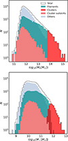 |
Fig. 1. Mass distributions of halos and their central galaxies in TNG300. Top panel: Distribution of total halo masses (Mh). Bottom panel: Stellar mass (M★) distribution of central galaxies. In both panels, the total sample is represented by a solid black line, while different environmental subsets are indicated as follows: filaments are shown in green, clusters in red, cluster outskirts in pink, and others in light blue. |
For cosmic web analysis in the SDSS spectroscopic survey, we utilised the identification done by Malavasi et al. (2020a) using the DisPerSE method. This approach followed the same procedure as that used for simulation data while also considering the observational nature of the data and accounting for projection effects. The results of this implementation are publicly available and the derived filament catalogues have been utilised in several studies, including those by Malavasi et al. (2020b), Tanimura et al. (2020a, b), and Bonjean et al. (2020). In this work, we use the 3σ persistence catalogue based on the Legacy North SDSS galaxy distribution (with smoothed density) consistent with what we employ in TNG300.
To define large-scale environments in SDSS DR18 in a manner analogous to those used in simulations and compare our results, we combined the group catalogue obtained using the method of Rodriguez & Merchán (2020) with the DisPerSE implementation of Malavasi et al. (2020a). We selected central galaxies brighter than −19.5 in the r band. This approach allowed us to use the same definitions as before: clusters were identified using the same mass threshold based on the mass provided by the group identification method; the remaining environments were defined following the same guidelines. It is important to note that this environment identification in redshift space introduces systematic effects like the fingers-of-God elongation and line-of-sight projection artefacts. These effects may dominate the uncertainty budget in environment classification, particularly for cluster regions and filament connectivity.
3. Alignment definitions
3.1. Simulation
In this work, we investigate the alignment properties of central galaxies, focusing on the brightest (and most massive) group galaxies (BGGs). Building upon our previous methodological developments (Rodriguez et al. 2023, 2024) and following established best practices for shape measurement (Zemp et al. 2011; Bassett & Foster 2019), we analysed these systems using exclusively stellar and DM particles enclosed within twice the half-DM mass radius. We computed the inertia tensor (Ii,j) of the BGGs as
 (1)
(1)
where i and j correspond to the three spatial axes of the simulated box, i.e. i,j = 1,2,3. The term mn represents the mass of the n-th, while  and
and  denote the positions of the n-th particle along the i-th and j-th axes, respectively. These particle positions are measured relative to the centre of the sub-halo to which the particle belongs, defined as the position of the particle with the minimum gravitational potential energy. Let ra, rb, and rc be the three normalised eigenvectors of Ii,j corresponding to the major, intermediate, and minor axes, respectively. From these directions, we defined three angles that provide an insight into the internal alignment of the BGG and its alignment with the other group members, referred to as satellites.
We begin by introducing the first angle, which quantifies the alignment of the internal components of the BGG. In this approach, we use the angle between the principal shape axes corresponding to DM and stars, which we refer to as θint, is illustrated in the first diagram of Fig. 2 and is defined as
 (2)
(2)
where θint,k is the angle between the k-th semi-axis calculated using DM (rdm,k) and the corresponding semi-axis determined using stars (rstars,k).
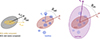 |
Fig. 2. Schematic showing the angles used in this work to study alignments. From left to right, the angles θint, θsat, and θch are displayed. The first, θint, represents the alignment between the stellar and DM components of the BGG. The second, θsat, corresponds to the angle between the principal axes of the BGG and the position of a satellite galaxy. Finally, θch describes the angle between the principal axes of the BGG and those of the host DM halo of the group. |
The second angle we define is θsat, which is used to analyse the distribution of galaxies in relation to a specific axis of the BGG (see the second diagram of Fig. 2). This angle was calculated using the following equation:
 (3)
(3)
In this equation, xBGG represents the position of the BGG, while xsat refers to the position of a satellite galaxy. The term rdm/stars,k denotes the k-th eigenvector of the BGG’s shape, which can be calculated using either DM or stars. Essentially, this angle describes the orientation of the satellite’s relative position with respect to the BGG’s principal axes.
To further explore the alignments and to complement the two previous definitions, we introduce a third angle, denoted as θch, which is illustrated in the third diagram of Fig. 2. This angle is defined as the angle between the principal axes of inertia, which are calculated using the positions and masses of the DM particles in the group, and the axes corresponding to the BGG:
 (4)
(4)
where k denotes the semi-axis considered and rc and rh represent the normalised eigenvectors corresponding to the BGG and the group, respectively.
As we are going to study the behaviour of these three angles statistically throughout this work, it is important to bear in mind that, in the case of a random spatial distribution, they give an average value of 60°. That is, values greater than 60° indicate a misalignment, while ones less than 60° suggest an alignment.
3.2. SDSS
To measure the alignments in the SDSS, we introduced angles that are analogous to the ones defined in simulations, while considering the projection limitations of the catalogues. The direction of the main shape axis of the BGG is represented by the position angle calculated from its brightness distribution, as provided by the SDSS. The direction of the group is defined by the position angle that corresponds to the eigenvector of the semi-major axis, which is obtained from the two-dimensional inertia tensor using the projected positions of its member galaxies. From this information, the projected counterpart of θch is called φch, calculated simply as the difference between the two angles.
A similar approach was applied to the analogous angle, θsat, which we denote as φsat. In this case, we considered the position angle of the projected radius vector of the member galaxies in relation to the main shape axis of the BGG provided by the survey.
It is worth mentioning that, in this case, since these angles are measured in projection, the average values corresponding to a random distribution are 45°. Moreover, due to the lack of information regarding the DM distribution in the BGG halo, we cannot observe an equivalent of θint. In this article, we first focus on the simulation, reserving the analysis corresponding to the SDSS for the final section.
4. Dependence of alignments on mass
In this study, we aim to analyse the behaviour of the angles discussed earlier with respect to the local and global environments surrounding central galaxies. The mass of a galaxy group serves as the primary indicator of this environment. This mass is closely linked to the astrophysical processes that influence the formation and evolution of the galaxies within the group. For instance, characteristics such as the merger rate, mean density, and colour of the central galaxy show a strong dependence on mass (e.g. Shankar et al. 2006; Contreras et al. 2015; Wechsler & Tinker 2018; Man et al. 2019). This relationship is also evident in several scaling relations (e.g. Rodriguez et al. 2021; Behroozi et al. 2010).
In Rodriguez et al. (2022, 2023, 2024), we explore the alignments of galaxies, focusing specifically on their colour dependence to compare our findings with the results obtained from observations and simulations. However, those studies show that the dependence on mass of the alignments calculated using the correlation function is equally as strong as, if not stronger than, that on colour. Therefore, the first analysis we chose to conduct in the present paper examines the relationship between the alignment of the central galaxies in our sample and the mass of the halos in which they are located.
In the left panel of Fig. 3, we observe that the angle θint decreases as the mass increases for both the major and the minor axes. The minor axis exhibits values lower than the major axis for masses below ∼1014 M⊙, while both axes show similar values for masses above this threshold. This angle represents the alignment between the stars and the DM halo they inhabit, indicating that the major and minor axes of both the stars and the DM halo tend to become more aligned as the mass of the halo increases. Additionally, it suggests that for lower-mass halos, the minor axes are more closely aligned with each other than their respective major axes. The noticeable difference in alignment between the major and minor axes of galaxies residing in less massive halos can be attributed to their tendency to be spiral (oblate) (see, for example, Rodriguez et al. 2024). This morphology results in a more clearly defined minor axis compared to the other two axes, which are quite similar and lie within the same plane. In the most massive end, the predominant morphology is triaxial, meaning that the three axes are clearly defined, with no differences in alignment between the minor and major axes. This behaviour of internal alignment may arise from the fact that the processes involved in the formation and evolution of galaxies vary depending on their mass. This variation underscores the complex nature of galaxy development, highlighting how halo mass plays a crucial role in shaping galaxies.
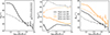 |
Fig. 3. Relation between the alignment and the mass of the halo in which the central galaxies of the sample are located. The left, centre, and right panels present this relation for angles θint, θsat, and θch respectively. In all panels, solid lines represent the major axis, while dotted lines represent the minor axis. Additionally, where possible, measurements based solely on stellar information are indicated in yellow. Error bars were calculated using the standard deviation of the mean. The left panel illustrates the direction of increasing alignment. This feature is consistent across all panels displaying alignments in this figure and the subsequent ones. |
The central panel of Fig. 3 illustrates the relationship between θsat and mass. It is evident that this angle, measured with respect to the major (resp. minor) axis, shows a strong alignment (resp. misalignment) across the entire range of masses. Examining the DM estimates (black curves), we observe that unlike many other halo properties, θsat does not show a strong dependency on mass. Only for lower masses, around ∼1012 M⊙, alignment in both axes seems to be a small feature. It is important to note that this angle was calculated for each satellite individually. As a result, at the lower halo mass end, there are many groups with only a few members. In contrast, at the higher-mass end, there are fewer clusters but a greater number of satellites. Estimating the axes of the central galaxy using stellar material yields measurements closer to 60°. Here, the alignment of the major axis with mass increases, but the minor axis shows the opposite trend. This behaviour is expected since, as is illustrated in the left panel described above, the stars are misaligned in relation to their own DM halo, and this misalignment decreases as halo mass increases. As a result, measurements derived from DM and stars tend to converge and resemble each other as halo mass increases. The results of θsat indicate that satellite galaxies are preferentially distributed around the major axis.
We finally focus on the angle between the central galaxy’s shape with that of the host group, θch, in the right panel of Fig. 3. Is it clear that this angle significantly decreases with mass, showing a progressive alignment between the shape of the galaxy and its associated group as halo mass increases. This trend is observed for both the major and minor axes when analysing the shapes of DM and stellar components. Notably, measurements taken from stars exhibit greater misalignment than those related to DM. This discrepancy may result from the internal misalignment represented by θint, indicating that the DM of the BGG is more closely aligned with the shape of the host halo than the stars of the BGG (see Figs. 7 and 8 in Rodriguez et al. 2023).
Previous studies have shown that central galaxies are aligned with their surroundings, and this alignment is more pronounced when considering DM instead of just stars. In this section we have analysed how these alignments depend on halo mass and found that both the internal orientation angle (θint) and the orientation angle of the central galaxy shape with respect to that of the host halo (θch) increase with mass. In contrast, the distribution of satellites (θsat) does not exhibit a significant dependence on mass.
5. Environmental effects
Having established the relationship between the studied angles and halo mass, we next analysed how the large-scale environment and its characteristics influence these alignments in filaments, clusters, cluster outskirts, and others. Given that clusters occupy uniquely the high mass-end of the halo mass distribution, the trends for galaxies in these structures are dominated by the mass effect described above. Regardless, we include this information for the sake of completeness. In contrast, the remaining environments are populated by objects within a similar and overlapping halo mass range, as is illustrated in Fig. 1, enabling the exploration of any specific trends arising from environmental effects while keeping the halo mass fixed. To begin with, we analysed the alignments taking into account the axes defined using DM particles. This builds on the results derived from the black curves presented in the Fig. 3.
In the left panel of Fig. 4, we illustrate how θint varies as a function of halo mass across different environments. At a glance, we can see that in all environments the same trend with halo mass is observed as in the overall sample of the previous section and figure. Along the major axis (solid lines), we observe that around 1013 M⊙ stellar material and DM exhibit a lower alignment in filaments than others, as the θint values for galaxies in filaments are ∼4° higher than in others. Note that the cluster outskirts shows noisy results, mainly because there are only 2122 halos in this environment. In contrast, galaxies in others demonstrate the lowest degree of alignment at lower masses. Additionally, within the halo mass range from approximately 1012 to 1013 M⊙, central galaxies in filaments are less aligned compared to those in other environments. Although the above results are statistically significant, the differences found are minimal across the different environments compared to the trends with mass, which are the dominant ones driving the alignments.
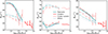 |
Fig. 4. Relation between the alignment of central galaxies and the mass of the halos in which they are located across different large-scale environments. The left, centre, and right panels illustrate this relationship for angles θint, θsat, and θch, respectively. In all panels, solid lines indicate the major axis, while dotted lines represent the minor axis. The lines shown in green, red, pink, and light blue correspond to halos in filaments, clusters, cluster outskirts, and other environments, respectively. The axes were measured using the DM particles and error bars were calculated using the standard deviation of the mean. In all panels, solid lines represent the major axis, while dotted lines represent the minor axis. |
In the middle panel of Fig. 4, we observe a variation in the alignment of θsat with cosmic environment. Galaxies classified as others show a somewhat stronger alignment along the major axis, followed by those located in filaments, while galaxies on the cluster outskirts exhibit a weaker alignment. Conversely, the results for the minor axis present an opposite trend. With this in mind, the results suggest that the alignment of satellite galaxies increases as the density decreases.
For the different environments, the right panel of Fig. 4 shows the relationship between θch and mass. For the minor axis (dotted lines), it is observed that there is a lower alignment for the centrals in cluster outskirts, followed in alignment by the filaments and, finally, by those in others. On the major axis, the trends are similar although the results for cluster outskirts are noisy. This would indicate that, like θsat, the DM halos of central galaxies are increasingly aligned with the host halos, when the environment is less and less hostile.
We now analyse the results for θsat and θch using stellar particles. They are shown in Fig. 5. In general, we observe that in both panels, the differences obtained between environments are smaller than the corresponding results for the case where the axes are defined using the DM distribution. For θsat, it is not possible to detect any variation in the alignment with the environment given the uncertainties in the measurements. In the case of θch (lower panel), although there appear to be some differences similar to those observed with DM. However, it should be borne in mind that, to compare it with observations, we would need to consider the effects of projection, the distortions produced by the redshift space, and the errors inherent in the measurements or the environment detection, which together contribute to an increase in the errors of the angles we are studying.
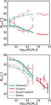 |
Fig. 5. Same format as in Fig. 4, but presenting the alignment of the main axes measured with the stellar component of the central galaxies. |
5.1. Variations with filament density
The previous results suggest a second-order connection between large-scale environments and the alignment of central galaxies. We now further explore this connection by addressing potential differences within the filaments class, namely by disentangling any variation in alignment as a function of the density of the filaments hosting central galaxies. To do this, we define filament density based on the galaxies located within 2 Mpc of the filament’s axis, considering a cylinder of the same radius, with length corresponding to the total length of the segments that comprise the filament.
In Fig. 6 we analyse the behaviour of the angles θint, θsat, and θch by dividing the filaments based on their density. Two samples were taken using the first and fourth quartiles of the filament densities, corresponding to 24.5 and 82.7 Mpc−3, respectively. Note that, to calculate this density, we considered all galaxies with stellar mass greater than 108.5 M⊙. Darker lines represent higher-density filaments, while lighter lines indicate lower-density ones. In the left panel, we examine the alignment between DM and stars (θint). For denser filaments, the stellar component is less aligned with its DM halo along the major axis, particularly at higher masses. In contrast, the minor axes exhibit the opposite trend, with greater alignment in denser environments. This is clearly shown in the lower panel, which quantifies the ratio of angles between low- and high-density filaments, θlow/θhigh. For the major axis (solid line), we observe differences of up to 20% at high masses, while the minor axis (dashed line) shows smaller differences of around 10% at low masses. The middle and right panels present θsat and θch, respectively. Both panels show that for both minor and major axes, there is a greater alignment in less dense filaments. In summary, the only exception to this trend is the alignment θint for the minor axis at lower masses, which behaves differently than the other alignments. Regarding the ratio of angles between low- and high-density filaments for θsat, our analysis demonstrates that only the major axis is responsive to filament density, showing consistent differences of approximately 10% throughout the halo mass range. Furthermore, the ratio for θch remains similar for both axes and increases with mass, spanning from very low values to greater than 20%. These results underscore the strong effect of different filament environments on the alignment of central galaxies with respect to the three different reference scales explored in this paper.
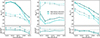 |
Fig. 6. Dependence on halo mass the angles θint (left), θsat (centre), and θch (right) for central galaxies located in filaments of varying densities. Darker lines represent the highest density quartile, while lighter lines correspond to the lowest. In all panels, solid lines represent the major axis, while dotted lines represent the minor axis. The lower panels show the ratio between the results at different densities. |
The results indicate that in the outermost regions of the halo traced by θsat and θch, the denser filaments generate a misalignment with respect to the major and minor axes of the central galaxy. On the other hand, in the innermost regions (traced by θint), DM and stars tend to align with the minor axis of the galaxy.
5.2. Variations with local density
At this stage, a key question that emerges is whether the filaments (as physical structures) are directly influencing the alignments, or whether we are simply measuring local density effects; in other words, whether the filaments or the local environment are responsible for affecting the alignments. Therefore, it is important to examine how much these samples differ in local density.
To address this issue, we estimated the local density by calculating the density of DM within a sphere of radius 5 Mpc centred around each BGG. We compared the local density distributions of central galaxies found in low- and high-density filaments, as is illustrated in Fig. 7. We present the results across four halo mass ranges to avoid potential biases associated with the mass variability. Due to the significant differences in local density observed between the two samples, we found that adjusting for local density resulted in alignment differences that closely resembled those shown in Fig. 6, which classifies galaxies according to filament density (we do not display this figure here because it does not provide relevant information).
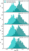 |
Fig. 7. Local density distribution at 5 Mpc for central galaxies found in low- and high-density filaments. |
We take a step further and focus now on the differences between centrals in filaments and those in others, i.e. the most under-dense cosmic environments. Figure 8 illustrates the local density distribution for those galaxies classified as belonging to filaments and others. As can be expected, the distributions differ significantly, with the filaments typically being much denser. In order to determine whether the presence of filaments has any effect on the alignments beyond local density effects, we made the two samples comparable by selecting a subsample of BGGs from the others that match the density distribution of the filament sample. This is illustrated by the dotted lines in Fig. 8.
 |
Fig. 8. Local density distribution at 5 Mpc for central galaxies found in filaments and those classified as others. The dotted line represents the distribution of galaxies selected from the others that correspond to those in filaments. |
Following the same approach as in the previous sections, Fig. 9 shows the results of the alignments for the BGGs in filaments (darker lines) and the mimic sample of other (lighter lines). In the innermost regions of the halo, when analysing θint, we observe that, at an equal local density, the differences between the field and the filaments are equivalent to those in Fig. 3, where the local density was not matched. This suggests that the observed differences are indeed due to the presence of the filament. As for the distribution of satellites around the BGG, represented by θsat, the central panel clearly illustrates that there are no significant differences when comparing the filament categories with the others, both with equal distribution of local densities. However, when analysing θch, it is observed that, at equal local density, the presence of the filament reduces the alignment on both axes, although the differences are not as marked as in Fig. 3. This suggests that the filament influences the alignment of the DM halo but not so much the distribution of satellite galaxies, or at least not to a level detectable with the sensitivity of our experiment.
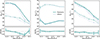 |
Fig. 9. Using the same format as Fig. 6, results are shown for central galaxies in filaments or others with the same local density distribution. |
6. SDSS
Numerical simulations are important tools because they allow for the analysis of complex phenomena and enable highly accurate predictions. One of their key advantages is that they are not influenced by observational biases that can affect studies relying solely on observed data. However, it is essential to compare theoretical predictions with actual observations to validate the results and draw reliable conclusions. In this section we analyse the alignments of central galaxies in the SDSS. To do this, we use the data and the angles defined in Sects. 2.2 and 3.2, respectively.
The first step is to measure how the alignments depend on mass. In this context, we examined the projected versions of θsat and θch, which are denoted as φsat and φch. Since the data we are using does not provide information about the DM content of the BGG, it is not possible to obtain the internal alignment. To calculate the shape of the group in the catalogue, we only have the member galaxies provided by our identifier. Generally, the number of members in these groups is relatively low; it is uncommon to find groups with more than ten members. Therefore, to maximise our sample size and obtain a reasonable estimate of the main axes, we selected groups with at least four members for our shape calculations, which we used to study φch.
The results are shown in the upper panels of Fig. 10, in which we only present the ones corresponding to the major axis of the BGG. As these angles are two-dimensional measurements, the results regarding the minor axis are complementary.
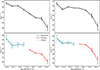 |
Fig. 10. SDSS measurements of the alignments of the major axis of the central galaxies with the location of the satellite galaxies (φsat) and of the major axis of the central galaxies with the major axis of the group to which they belong, measured with the member galaxies (φch). The upper panels show the total sample and its dependence on mass, while the lower panels show those corresponding to different environments of the cosmic web. In all panels, error bars represent the standard deviation of the mean. |
We first note that, despite the projection, we recover the trends detected in the simulations, as the alignment of the satellites φsat (shown in the upper left panel) shows a strong dependence on the mass. Similar to the simulations, no alignment is observed in low-mass systems; however, alignment significantly increases as halo mass increases (for reference, see measurements indicated by the yellow lines in Fig. 3). It is remarkable to find this dependence in the observations and that it agrees with the simulations. Indeed this result supports the reliability of the abundance matching procedure, which assigns masses in the group catalogue based solely on luminosity ranking and aims to provide a proxy for the mass, rather than an exact measurement.
In the upper right panel of Figure 10, we show the projected alignment of the BGG shape with respect to the halo shape, φch. Once again, the behaviour of φch as a function of the halo mass resembles that of the simulations: for low masses, the alignment is undetectable, whereas for high masses, it increases. It should be emphasised that, besides the uncertainties in determining the mass, the shapes are estimated with very few members and, therefore, the direction of the major axis of the group has significant uncertainty, unlike the simulations where the shape is determined with greater precision using numerous DM particles.
Based on our observations, we have provided observational confirmation of an important relationship between galaxy alignments and their mass. The next logical step is to investigate how these alignments depend on their environmental conditions on a large scale. For this analysis, we focus exclusively on three types of environments: filaments, clusters, and others. We are omitting cluster outskirts due to the limited number of galaxies in that category, which prevents us from obtaining reliable results. The bottom panels of Fig. 10 show the corresponding results for each environment.
As is observed, it is not possible to differentiate the alignments between the trends of filaments and others environments. This is not surprising, given several predictable factors. First, simulations indicate that stars are misaligned with their halo (see Fig. 6), which causes an attenuation in the signal we detect between the DM halo of the BGG and the group’s halo. Second, the identification of environments is less precise compared to simulations due to known observational biases. Considering these factors, which influence how galaxies are assigned to different environments, we assessed the impact of projected distance cuts on our results by testing several definitions of filament thickness. However, the results remained consistent with those presented in Fig. 10, convincing us to keep the original definitions.
7. Summary and conclusions
This study builds on our previous findings (Rodriguez et al. 2022, 2023) to explore how the mass of host halos and the locations of galaxies, whether in clusters, filaments, cluster outskirts, or other environments, affect these alignments.
We analysed how three different angles characterise the alignment of central galaxies with their multi-scale environment to understand their relation to the structure on different scales. First, we studied the alignment between the stellar and DM components of the central galaxy (θint), which provides information on the internal alignment. Second, we examined the angle between the satellite galaxies and the shape axes of the central galaxy (θsat), allowing us to characterise the distribution of stellar material within the halo in which the group resides. Finally, we investigated the alignment between the shape axis of the central galaxies and that of the group’s host halo (θch), providing information on the connection between galaxy and structure on larger scales. These angles are illustrated in Fig. 2, which provides a schematic representation of their definitions. These analyses let us explore how the surroundings and multi-scale physical processes influence the angles characterising the central galaxies.
First, we performed our analysis using the TNG300 hydrodynamical simulation. We explored how each angle depended on the halo mass. We found that both θint and θch – measured using the shape axes of the central galaxy defined by either the DM or stellar distributions – exhibit a clear trend of decreasing with halo mass (see Fig. 3). The first one suggests that, internally, the stellar component becomes more tightly coupled with DM as the halo mass increases. Similarly, from θch we can infer that the DM and stellar components of the central galaxy show a stronger alignment with the DM of the host halo as mass grows. In contrast, θsat does not demonstrate a clear dependence on mass when measured using the DM axes. When we consider the axes defined by the stellar distribution, a clear increasing trend with halo mass emerges. However, in all cases in which we measure the angles using the axes defined by stellar distribution, we find that it is systematically weaker than when measured using the DM axes. This suggests that while the stellar structure somewhat follows the DM, its degree of alignment with its surroundings is less pronounced. This could mean that the astrophysical processes affecting stars are more complex than the ones influencing DM, which is reflected in their alignments. These results expand on previous works, such as Valenzuela et al. (2024), in which the authors study central galaxy shapes in the Magneticum simulation and conclude that stellar and DM shapes are correlated at internal scales, but the inner halo appears to be decoupled from the outer halo. We find that the strength of both the internal stellar–sub-halo and the sub-halo–host halo alignment are strongly coupled in the more massive halos, and the large-scale structure environment impacts more on the sub-halo–host halo alignment than on the internal alignment.
Another analysis we conducted was the study of the variation in alignments as a function of halo mass across different environments of the cosmic web (see Fig. 4). We classified these environments into four categories: clusters, filaments, cluster outskirts, and a category labelled others, which includes voids and walls. As was expected, the most massive central galaxies – which also exhibit the strongest alignments – are by definition in clusters, while the other three environments host central galaxies of lower masses. We found significant differences between environments, suggesting that alignments depend on large-scale structure. Since we compared galaxies at fixed mass, the detected variations reflect the impact of the environment beyond the effect of the host halo mass. While the mass of the host halo largely influences alignments, the location in the most hostile environments of the cosmic web appears to disrupt these alignments at a fixed halo mass. Furthermore, since our previous analyses were based on DM, we investigated whether these differences persisted when measuring the principal axes of central galaxies using their stellar component (Fig. 5). We observed that the differences decreased compared to the ones found with DM, indicating that environmental influences are more pronounced in the DM structure than in the stellar distribution.
To further explore the relationship between alignments and the environment, we specifically analysed the case of filaments and studied the dependence of alignment angles on filament density (see Fig. 6), with the goal of probing the extreme diversity of the filament population. We found systematic variations with density, which suggests that filament properties influence the alignments of central galaxies consistent with the previous analysis, i.e. central galaxies in denser filaments are more misaligned. This finding led us to investigate whether the local density or the presence of the filaments themselves is the determining factor. As was expected, we found a strong correlation between filament and local density (see Fig. 7). This suggests that the effects observed in different environments could be associated with the characteristic local density of each region, rather than the presence of these specific structures. To address this question, we selected central galaxies in the areas labelled as others with a local density distribution similar to that of filaments (see Fig. 8). In this way, any detected differences should be attributed to effects related to their location in different regions of the cosmic web (see Fig. 9). Thus, we identified that, when analysing θint, there are differences in the alignments between the stellar and DM components when central galaxies are located in filaments or field at the same local density. However, the distribution of satellite galaxies, in terms of θsat, does not seem to be affected by the presence of these structures. Additionally, the alignment in θch also shows less coherence when the central galaxy is in filaments compared to the field. The results indicate that filaments cause a misalignment effect on DM host halos and the central galaxies within them, particularly affecting their DM component. In contrast, the positions of satellite galaxies appear to be less influenced by the presence of these filaments. This analysis showed that, in general, local density is the driving factor in the alignments of central galaxies, and that the position within the large-scale environment plays a secondary, marginal role.
To contrast with the results of the TNG300 simulations, we performed a similar analysis using SDSS data. First, we examined the alignments as a function of halo mass (see Fig. 10) and found a clear dependence, similar to what we observed in the simulations. This finding is particularly significant given the numerous observational biases inherent in SDSS data that could potentially obscure the signal, unlike in simulations where such biases are absent. The consistency between the two analyses underscores the reliability of group identification and halo mass assignments in the observational data. Additionally, it suggests that the physical effects that influence galaxy alignments in the real Universe are reflected in the simulations. Secondly, we investigated whether the differences observed between environments in the simulations were also present in the observational data, focusing on three environments: clusters, filaments, and others. However, we did not detect significant differences, likely due to observational biases that blur the effects identified in simulations. Nevertheless, it would be interesting to explore this further using alternative filament and void identification methods applied to future observational data.
In conclusion, this study has deepened our understanding of the alignments of central galaxies concerning their environment, both internally and on larger scales, using hydrodynamical simulations and observational data. The results confirm that the halo mass, and environment (both local and, to a lesser extent, large-scale), play a crucial role in determining these alignments. However, open questions remain about how other factors, such as the processes of galaxy formation and evolution, might influence these patterns. For example, Xu et al. (2023b) analysed the alignment between the principal axes of the stellar component and the host halo as a function of mass, and showed that fixing the ex situ stellar mass fraction almost eliminates the alignment’s dependence on halo mass, meaning that mass accretion processes strongly influence the alignments. Also, other studies using the SAMI and MaNGA surveys have established that there exists a relationship between the stellar mass and the alignment of galaxies’ angular momentum with filaments, and that some evolutionary processes such as bulge growth, active galactic nucleus activity, and mergers play an important role in producing the so-called spin flip effect (Welker et al. 2020; Kraljic et al. 2021; Barsanti et al. 2022, 2023, 2025). Given that a galaxy’s shape orientation can be related to its stellar angular momentum, there may be a connection between the spin–filament alignment and the axis alignments studied in this work. Nonetheless, caution is needed when making comparisons, as these are different types of alignments. Therefore, future research projects could explore in more detail the impact of the accretion history of galaxies or the relationship between a galaxy’s morphology and its alignment in different environments. Additionally, it would be beneficial to validate these findings through larger-volume simulations such as Flamingo (Schaye et al. 2023) or MillenniumTNG (Pakmor et al. 2023), which would enhance the statistical analysis. Exploring new methods of identifying structures in observational data would also help refine our understanding of the connection between galaxies and the cosmic web. This work is particularly timely, as new data from upcoming spectroscopic surveys such as the Dark Energy Spectroscopic Instrument (DESI), Euclid, and the Prime Focus Spectrograph (PFS) will soon be available. These surveys will provide unprecedented statistics and resolution, enabling rigorous tests of our predictions and offering new insights into galaxy alignments within the cosmic web.
Acknowledgments
The authors wish to thank the anonymous referee for her/his report that helps us to improve this manuscript. FR, MM and AVMC thanks the support by Agencia Nacional de Promoción Científica y Tecnológica, the Consejo Nacional de Investigaciones Científicas y Técnicas (CONICET, Argentina) and the Secretaría de Ciencia y Tecnología de la Universidad Nacional de Córdoba (SeCyT-UNC, Argentina). FR and ADMD thank the ICTP for their hospitality and financial support through the Junior Associates Programme 2023–2028 and Senior Associates Programme 2022–2027, respectively. DGE acknowledges Volker Springel for the financial support that facilitated the research visit during which part of this work was conducted. MCA acknowledges support from ANID BASAL project FB210003. ADMD thanks Fondecyt for financial support through the Fondecyt Regular 2021 grant 1210612.
References
- Agustsson, I., & Brainerd, T. G. 2010, ApJ, 709, 1321 [Google Scholar]
- Ahumada, R., Prieto, C. A., Almeida, A., et al. 2020, ApJS, 249, 3 [Google Scholar]
- Alfaro, I. G., Rodriguez, F., Ruiz, A. N., Luparello, H. E., & Lambas, D. G. 2022, A&A, 665, A44 [NASA ADS] [CrossRef] [EDP Sciences] [Google Scholar]
- Almeida, A., Anderson, S. F., Argudo-Fernández, M., et al. 2023, ApJS, 267, 44 [NASA ADS] [CrossRef] [Google Scholar]
- Ando, M., Shimasaku, K., & Ito, K. 2023, MNRAS, 519, 13 [Google Scholar]
- Barsanti, S., Colless, M., Welker, C., et al. 2022, MNRAS, 516, 3569 [NASA ADS] [CrossRef] [Google Scholar]
- Barsanti, S., Colless, M., D’Eugenio, F., et al. 2023, MNRAS, 526, 1613 [Google Scholar]
- Barsanti, S., Croom, S. M., Colless, M., et al. 2025, MNRAS, 538, 2660 [Google Scholar]
- Bassett, R., & Foster, C. 2019, MNRAS, 487, 2354 [Google Scholar]
- Behroozi, P. S., Conroy, C., & Wechsler, R. H. 2010, ApJ, 717, 379 [Google Scholar]
- Bonjean, V., Aghanim, N., Douspis, M., Malavasi, N., & Tanimura, H. 2020, A&A, 638, A75 [NASA ADS] [CrossRef] [EDP Sciences] [Google Scholar]
- Bray, A. D., Pillepich, A., Sales, L. V., et al. 2016, MNRAS, 455, 185 [NASA ADS] [CrossRef] [Google Scholar]
- Catelan, P., Kamionkowski, M., & Blandford, R. D. 2001, MNRAS, 320, L7 [NASA ADS] [CrossRef] [Google Scholar]
- Codis, S., Pichon, C., & Pogosyan, D. 2015, MNRAS, 452, 3369 [Google Scholar]
- Conroy, C., Wechsler, R. H., & Kravtsov, A. V. 2006, ApJ, 647, 201 [Google Scholar]
- Contreras, S., Baugh, C., Norberg, P., & Padilla, N. 2015, MNRAS, 452, 1861 [CrossRef] [Google Scholar]
- Davis, M., Efstathiou, G., Frenk, C. S., & White, S. D. M. 1985, ApJ, 292, 371 [Google Scholar]
- Desai, D. D., & Ryden, B. S. 2022, ApJ, 936, 25 [CrossRef] [Google Scholar]
- Dolag, K., Borgani, S., Murante, G., & Springel, V. 2009, MNRAS, 399, 497 [Google Scholar]
- Galárraga-Espinosa, D., Aghanim, N., Langer, M., Gouin, C., & Malavasi, N. 2020, A&A, 641, A173 [EDP Sciences] [Google Scholar]
- Galárraga-Espinosa, D., Garaldi, E., & Kauffmann, G. 2023, A&A, 671, A160 [NASA ADS] [CrossRef] [EDP Sciences] [Google Scholar]
- Ganeshaiah Veena, P., Cautun, M., Tempel, E., van de Weygaert, R., & Frenk, C. S. 2019, MNRAS, 487, 1607 [NASA ADS] [CrossRef] [Google Scholar]
- Ganeshaiah Veena, P., Cautun, M., van de Weygaert, R., Tempel, E., & Frenk, C. S. 2021, MNRAS, 503, 2280 [NASA ADS] [CrossRef] [Google Scholar]
- Genel, S., Vogelsberger, M., Springel, V., et al. 2014, MNRAS, 445, 175 [Google Scholar]
- Gonzalez, E. J., Rodriguez, F., Merchán, M., et al. 2021, MNRAS, 504, 4093 [NASA ADS] [CrossRef] [Google Scholar]
- Heavens, A., Refregier, A., & Heymans, C. 2000, MNRAS, 319, 649 [NASA ADS] [CrossRef] [Google Scholar]
- Hirata, C. M., Mandelbaum, R., Ishak, M., et al. 2007, MNRAS, 381, 1197 [NASA ADS] [CrossRef] [Google Scholar]
- Huchra, J., & Geller, M. 1982, ApJ, 257, 423 [NASA ADS] [CrossRef] [Google Scholar]
- Joachimi, B., Cacciato, M., Kitching, T. D., et al. 2015, Space Sci. Rev., 193, 1 [Google Scholar]
- Johnston, H., Georgiou, C., Joachimi, B., et al. 2019, A&A, 624, A30 [NASA ADS] [CrossRef] [EDP Sciences] [Google Scholar]
- Kiessling, A., Cacciato, M., Joachimi, B., et al. 2015, Space Sci. Rev., 193, 67 [Google Scholar]
- Kirk, D., Brown, M. L., Hoekstra, H., et al. 2015, Space Sci. Rev., 193, 139 [Google Scholar]
- Kraljic, K., Duckworth, C., Tojeiro, R., et al. 2021, MNRAS, 504, 4626 [NASA ADS] [CrossRef] [Google Scholar]
- Kravtsov, A. V., Berlind, A. A., Wechsler, R. H., et al. 2004, ApJ, 609, 35 [Google Scholar]
- Lacerna, I., Rodriguez, F., Montero-Dorta, A. D., et al. 2022, MNRAS, 513, 2271 [NASA ADS] [CrossRef] [Google Scholar]
- Lagos, C. D. P., Stevens, A. R., Bower, R. G., et al. 2018, MNRAS, 473, 4956 [NASA ADS] [CrossRef] [Google Scholar]
- Libeskind, N. I., Hoffman, Y., Tully, R. B., et al. 2015, MNRAS, 452, 1052 [NASA ADS] [CrossRef] [Google Scholar]
- Maier, C., Haines, C. P., & Ziegler, B. L. 2022, A&A, 658, A190 [NASA ADS] [CrossRef] [EDP Sciences] [Google Scholar]
- Malavasi, N., Aghanim, N., Douspis, M., Tanimura, H., & Bonjean, V. 2020a, A&A, 642, A19 [NASA ADS] [CrossRef] [EDP Sciences] [Google Scholar]
- Malavasi, N., Aghanim, N., Tanimura, H., Bonjean, V., & Douspis, M. 2020b, A&A, 634, A30 [NASA ADS] [CrossRef] [EDP Sciences] [Google Scholar]
- Man, Z. -Y., Peng, Y. -J., Shi, J. -J., et al. 2019, ApJ, 881, 74 [Google Scholar]
- Merchán, M. E., & Zandivarez, A. 2005, ApJ, 630, 759 [CrossRef] [Google Scholar]
- Montero-Dorta, A. D., & Rodriguez, F. 2024, MNRAS, 531, 290 [NASA ADS] [CrossRef] [Google Scholar]
- Morse, M. 1934, The Calculus of Variations in the Large (American Mathematical Soc.), 18 [Google Scholar]
- Nelson, D., Springel, V., Pillepich, A., et al. 2019, Comput. Astrophys. Cosmol., 6, 2 [Google Scholar]
- Otter, J. A., Masters, K. L., Simmons, B., & Lintott, C. J. 2020, MNRAS, 492, 2722 [NASA ADS] [CrossRef] [Google Scholar]
- Pakmor, R., Springel, V., Coles, J. P., et al. 2023, MNRAS, 524, 2539 [NASA ADS] [CrossRef] [Google Scholar]
- Pawlowski, M. S. 2018, Mod. Phys. Lett. A, 33, 1830004 [NASA ADS] [CrossRef] [Google Scholar]
- Paz, D. J., Stasyszyn, F., & Padilla, N. D. 2008, MNRAS, 389, 1127 [NASA ADS] [CrossRef] [Google Scholar]
- Paz, D. J., Sgró, M. A., Merchán, M., & Padilla, N. 2011, MNRAS, 414, 2029 [NASA ADS] [CrossRef] [Google Scholar]
- Perez, N. R., Pereyra, L. A., Coldwell, G., et al. 2024a, MNRAS, 528, 3186 [Google Scholar]
- Perez, N. R., Pereyra, L. A., Coldwell, G., et al. 2024b, MNRAS, 534, 2228 [Google Scholar]
- Pillepich, A., Springel, V., Nelson, D., et al. 2018a, MNRAS, 473, 4077 [Google Scholar]
- Pillepich, A., Nelson, D., Hernquist, L., et al. 2018b, MNRAS, 475, 648 [Google Scholar]
- Planck Collaboration XIII. 2016, A&A, 594, A13 [NASA ADS] [CrossRef] [EDP Sciences] [Google Scholar]
- Rodriguez, F., & Merchán, M. 2020, A&A, 636, A61 [NASA ADS] [CrossRef] [EDP Sciences] [Google Scholar]
- Rodriguez, F., Montero-Dorta, A. D., Angulo, R. E., Artale, M. C., & Merchán, M. 2021, MNRAS, 505, 3192 [NASA ADS] [CrossRef] [Google Scholar]
- Rodriguez, F., Merchán, M., & Artale, M. C. 2022, MNRAS, 514, 1077 [NASA ADS] [CrossRef] [Google Scholar]
- Rodriguez, F., Merchán, M., Artale, M. C., & Andrews, M. 2023, MNRAS, 521, 5483 [NASA ADS] [CrossRef] [Google Scholar]
- Rodriguez, F., Merchán, M., & Artale, M. C. 2024, A&A, 688, A40 [NASA ADS] [CrossRef] [EDP Sciences] [Google Scholar]
- Rodríguez-Medrano, A. M., Paz, D. J., Stasyszyn, F. A., et al. 2023, MNRAS, 521, 916 [CrossRef] [Google Scholar]
- Sales, L., & Lambas, D. G. 2004, MNRAS, 348, 1236 [NASA ADS] [CrossRef] [Google Scholar]
- Samuroff, S., Mandelbaum, R., Blazek, J., et al. 2023, MNRAS, 524, 2195 [Google Scholar]
- Schaye, J., Kugel, R., Schaller, M., et al. 2023, MNRAS, 526, 4978 [NASA ADS] [CrossRef] [Google Scholar]
- Shankar, F., Lapi, A., Salucci, P., De Zotti, G., & Danese, L. 2006, ApJ, 643, 14 [NASA ADS] [CrossRef] [Google Scholar]
- Smith, R., Hwang, H. S., Kraljic, K., et al. 2023, MNRAS, 525, 4685 [NASA ADS] [CrossRef] [Google Scholar]
- Sousbie, T. 2011, MNRAS, 414, 350 [NASA ADS] [CrossRef] [Google Scholar]
- Sousbie, T., Pichon, C., & Kawahara, H. 2011, MNRAS, 414, 384 [NASA ADS] [CrossRef] [Google Scholar]
- Springel, V. 2010, MNRAS, 401, 791 [Google Scholar]
- Springel, V., White, S. D. M., Tormen, G., & Kauffmann, G. 2001, MNRAS, 328, 726 [Google Scholar]
- Stott, J. P. 2022, MNRAS, 511, 2659 [NASA ADS] [CrossRef] [Google Scholar]
- Tanimura, H., Aghanim, N., Bonjean, V., Malavasi, N., & Douspis, M. 2020a, A&A, 637, A41 [NASA ADS] [CrossRef] [EDP Sciences] [Google Scholar]
- Tanimura, H., Aghanim, N., Kolodzig, A., Douspis, M., & Malavasi, N. 2020b, A&A, 643, L2 [EDP Sciences] [Google Scholar]
- Troxel, M. A., & Ishak, M. 2015, Phys. Rep., 558, 1 [NASA ADS] [CrossRef] [Google Scholar]
- Vale, A., & Ostriker, J. 2004, MNRAS, 353, 189 [NASA ADS] [CrossRef] [Google Scholar]
- Valenzuela, L. M., Remus, R. -S., Dolag, K., & Seidel, B. A. 2024, A&A, 690, A206 [NASA ADS] [CrossRef] [EDP Sciences] [Google Scholar]
- van de Weygaert, R., & Schaap, W. 2009, Data Analysis in Cosmology (Berlin: Springer) [Google Scholar]
- Vogelsberger, M., Genel, S., Springel, V., et al. 2014a, MNRAS, 444, 1518 [Google Scholar]
- Vogelsberger, M., Genel, S., Springel, V., et al. 2014b, Nature, 509, 177 [Google Scholar]
- Wang, Y., Yang, X., Mo, H. J., et al. 2008, MNRAS, 385, 1511 [NASA ADS] [CrossRef] [Google Scholar]
- Wang, K., Avestruz, C., Guo, H., Wang, W., & Wang, P. 2024, MNRAS, 532, 4616 [NASA ADS] [CrossRef] [Google Scholar]
- Wechsler, R. H., & Tinker, J. L. 2018, ARA&A, 56, 435 [NASA ADS] [CrossRef] [Google Scholar]
- Welker, C., Dubois, Y., Pichon, C., Devriendt, J., & Chisari, N. E. 2018, A&A, 613, A4 [NASA ADS] [CrossRef] [EDP Sciences] [Google Scholar]
- Welker, C., Bland-Hawthorn, J., van de Sande, J., et al. 2020, MNRAS, 491, 2864 [NASA ADS] [CrossRef] [Google Scholar]
- Xu, K., Jing, Y. P., & Gao, H. 2023a, ApJ, 954, 2 [NASA ADS] [CrossRef] [Google Scholar]
- Xu, K., Jing, Y. P., & Zhao, D. 2023b, ApJ, 957, 45 [NASA ADS] [CrossRef] [Google Scholar]
- Yang, X., Mo, H., Van Den Bosch, F. C., & Jing, Y. 2005, MNRAS, 356, 1293 [NASA ADS] [CrossRef] [Google Scholar]
- Yang, X., Van Den Bosch, F. C., Mo, H., et al. 2006, MNRAS, 369, 1293 [NASA ADS] [CrossRef] [Google Scholar]
- Zemp, M., Gnedin, O. Y., Gnedin, N. Y., & Kravtsov, A. V. 2011, ApJS, 197, 30 [Google Scholar]
- Zjupa, J., Schäfer, B. M., & Hahn, O. 2022, MNRAS, 514, 2049 [NASA ADS] [CrossRef] [Google Scholar]
All Figures
|
Fig. 1. Mass distributions of halos and their central galaxies in TNG300. Top panel: Distribution of total halo masses (Mh). Bottom panel: Stellar mass (M★) distribution of central galaxies. In both panels, the total sample is represented by a solid black line, while different environmental subsets are indicated as follows: filaments are shown in green, clusters in red, cluster outskirts in pink, and others in light blue. |
| In the text | |
|
Fig. 2. Schematic showing the angles used in this work to study alignments. From left to right, the angles θint, θsat, and θch are displayed. The first, θint, represents the alignment between the stellar and DM components of the BGG. The second, θsat, corresponds to the angle between the principal axes of the BGG and the position of a satellite galaxy. Finally, θch describes the angle between the principal axes of the BGG and those of the host DM halo of the group. |
| In the text | |
|
Fig. 3. Relation between the alignment and the mass of the halo in which the central galaxies of the sample are located. The left, centre, and right panels present this relation for angles θint, θsat, and θch respectively. In all panels, solid lines represent the major axis, while dotted lines represent the minor axis. Additionally, where possible, measurements based solely on stellar information are indicated in yellow. Error bars were calculated using the standard deviation of the mean. The left panel illustrates the direction of increasing alignment. This feature is consistent across all panels displaying alignments in this figure and the subsequent ones. |
| In the text | |
|
Fig. 4. Relation between the alignment of central galaxies and the mass of the halos in which they are located across different large-scale environments. The left, centre, and right panels illustrate this relationship for angles θint, θsat, and θch, respectively. In all panels, solid lines indicate the major axis, while dotted lines represent the minor axis. The lines shown in green, red, pink, and light blue correspond to halos in filaments, clusters, cluster outskirts, and other environments, respectively. The axes were measured using the DM particles and error bars were calculated using the standard deviation of the mean. In all panels, solid lines represent the major axis, while dotted lines represent the minor axis. |
| In the text | |
|
Fig. 5. Same format as in Fig. 4, but presenting the alignment of the main axes measured with the stellar component of the central galaxies. |
| In the text | |
|
Fig. 6. Dependence on halo mass the angles θint (left), θsat (centre), and θch (right) for central galaxies located in filaments of varying densities. Darker lines represent the highest density quartile, while lighter lines correspond to the lowest. In all panels, solid lines represent the major axis, while dotted lines represent the minor axis. The lower panels show the ratio between the results at different densities. |
| In the text | |
|
Fig. 7. Local density distribution at 5 Mpc for central galaxies found in low- and high-density filaments. |
| In the text | |
|
Fig. 8. Local density distribution at 5 Mpc for central galaxies found in filaments and those classified as others. The dotted line represents the distribution of galaxies selected from the others that correspond to those in filaments. |
| In the text | |
|
Fig. 9. Using the same format as Fig. 6, results are shown for central galaxies in filaments or others with the same local density distribution. |
| In the text | |
|
Fig. 10. SDSS measurements of the alignments of the major axis of the central galaxies with the location of the satellite galaxies (φsat) and of the major axis of the central galaxies with the major axis of the group to which they belong, measured with the member galaxies (φch). The upper panels show the total sample and its dependence on mass, while the lower panels show those corresponding to different environments of the cosmic web. In all panels, error bars represent the standard deviation of the mean. |
| In the text | |
Current usage metrics show cumulative count of Article Views (full-text article views including HTML views, PDF and ePub downloads, according to the available data) and Abstracts Views on Vision4Press platform.
Data correspond to usage on the plateform after 2015. The current usage metrics is available 48-96 hours after online publication and is updated daily on week days.
Initial download of the metrics may take a while.