| Issue |
A&A
Volume 699, July 2025
|
|
|---|---|---|
| Article Number | A232 | |
| Number of page(s) | 20 | |
| Section | Catalogs and data | |
| DOI | https://doi.org/10.1051/0004-6361/202554501 | |
| Published online | 14 July 2025 | |
Galaxies OBserved as Low-luminosity Identified Nebulae (GOBLIN): Catalog of 43 000 high-probability dwarf galaxy candidates in the UNIONS survey
1 Institute of Physics, Laboratory of Astrophysics, Ecole Polytechnique Fédérale de Lausanne (EPFL),
1290
Sauverny, Switzerland
2 Institute of Astronomy, Madingley Road, Cambridge CB3 0HA,
UK
3 Visiting Fellow, Clare Hall, University of Cambridge, Cambridge, UK
4 National Research Council of Canada, Herzberg Astronomy & Astrophysics Research Centre,
5071
West Saanich Road, Victoria BC V9E 2E7, Canada
5 Department of Physics and Astronomy, University of Waterloo, 200 University Avenue West,
Waterloo ON N2L 3G1, Canada
6 Institute for Astronomy, University of Hawaii,
2680 Woodlawn Drive, Honolulu, HI 96822, USA
7 Waterloo Centre for Astrophysics, University of Waterloo, Waterloo,
Ontario N2L 3G1, Canada
8 Perimeter Institute for Theoretical Physics,
31 Caroline St. North,
Waterloo,
ON N2L 2Y5,
Canada
9 LIRA, Observatoire de Paris, Universite PSL,
CNRS, Place Jules Janssen,
92195 Meudon,
France
10 UK Astronomy Technology Centre, Royal Observatory, Blackford Hill,
Edinburgh EH9 3HJ,
UK
⋆ Corresponding author: This email address is being protected from spambots. You need JavaScript enabled to view it.
Received:
12
March
2025
Accepted:
23
May
2025
Abstract
The detection of low-surface-brightness galaxies beyond the Local Group poses significant observational challenges, yet these faint systems are fundamental to our understanding of dark matter, hierarchical galaxy formation, and cosmic structure. Their abundance and distribution provide crucial tests for cosmological models, particularly regarding the small-scale predictions of ΛCDM. We present a systematic detection and classification framework for unresolved dwarf galaxy candidates in the large-scale Ultraviolet Near Infrared Optical Northern Survey (UNIONS) imaging data. The main survey region covers 4861 deg2. Our pipeline preprocesses UNIONS data in three (gri) of the five bands (ugriz), including binning, artifact removal, and stellar masking before employing the software MTOBJECTS (MTO) to detect low-surface-brightness objects. Following a set of parameter cuts using known dwarf galaxies from the literature and cross-matching between the three bands, we were left with an average of ∼360 candidates per deg2. With ∼4000 deg2 in g, r and i, this amounts to ∼1.5 million candidates that form our GOBLIN (Galaxies OBserved as Low-luminosity Identified Nebulae) catalog. For the final classification of these candidates, we finetuned the deep learning model ZOOBOT, which was pretrained based on labels from the Galaxy Zoo project. We created our training dataset by visually inspecting dwarf galaxy candidates from existing literature catalogs within our survey area and assigning probability labels based on averaged expert assessments. This approach captures both consensus and uncertainty among experts. When applied to all detected MTO objects, our method identified 42 965 dwarf galaxy candidates with probability scores of >0.8, of which 23 072 have probabilities exceeding 0.9. The spatial distribution of high-probability candidates reveals a correlation with the locations of massive galaxies (log (M∗/M⊙)≥ 10) within 120 Mpc. While some of these objects may have been previously identified in other surveys, we present this extensive catalog of candidates, including their positions, structural parameter estimates, and classification probabilities, as a resource for the community to enable studies of galaxy formation, evolution, and the distribution of dwarf galaxies in different environments.
Key words: methods: observational / techniques: image processing / catalogs / surveys / galaxies: abundances / galaxies: dwarf
© The Authors 2025
 Open Access article, published by EDP Sciences, under the terms of the Creative Commons Attribution License (https://creativecommons.org/licenses/by/4.0), which permits unrestricted use, distribution, and reproduction in any medium, provided the original work is properly cited.
This article is published in open access under the Subscribe to Open model. This email address is being protected from spambots. You need JavaScript enabled to view it. to support open access publication.
1 Introduction
Dwarf galaxies occupy the low-mass, low-luminosity end of the galaxy distribution and also represents the oldest and most numerous galaxy type in the Universe (Binggeli et al. 1990; Ferguson & Binggeli 1994). Dwarfs are small systems that contain gas, dust, dark matter, and up to a billion stars with total stellar masses ≤ 109 M⊙ (Bullock & Boylan-Kolchin 2017). They are the most dark matter-dominated galaxy type (e.g., Mateo et al. 1991; Walker et al. 2009; Collins et al. 2020), making them excellent laboratories for studying this puzzling component. In the ΛCDM standard model of cosmology, they are thought of as the fundamental building blocks of all galaxies, contributing to their formation via hierarchical merger (Frenk & White 2012). Thanks to the study of dwarf galaxies, we can gain important insights into how galaxies form and evolve over time (Revaz & Jablonka 2018).
Even though dwarfs are the most abundant galaxies in the Universe, their small size, low-surface-brightness, and faint nature pose a unique set of challenges for the detection of these elusive objects. Before the year 2004, nearly all then-known dwarf galaxies had been discovered and characterized via visual inspection of deep, wide-field photographic plates. Significant advancements in this area came from dedicated surveys utilizing the unique wide-field and high-resolution capabilities of instruments, such as the 2.5 m du Pont telescope at Las Campanas. These systematic investigations of clusters such as Virgo (e.g., Sandage & Binggeli 1984; Binggeli et al. 1985), Fornax (Ferguson & Sandage 1988; Ferguson 1989), and Centaurus (Jerjen & Dressler 1997), along with several nearby galaxy groups (Ferguson & Sandage 1990), were instrumental in establishing morphological classifications, substantially expanding the census of low-surface-brightness dwarfs, and providing foundational datasets for analyzing their populations and distributions (see also Ferguson & Binggeli (1994) for a review). As notable exceptions to this primary reliance on visual plate inspection, the dwarf galaxies Sextans and Sagittarius were found as stellar over-densities in automated surveys in 1990 and 1994, respectively (Irwin et al. 1990; Ibata et al. 1994). A stark discrepancy in the number count of Local Group (LG) dwarf galaxies between simulations and observations – the so-called “missing satellites” problem (Klypin et al. 1999; Moore et al. 1999) – enforced the previously noted need to gain a complete census of the nearby dwarfs (Willman 2010; MacGillivray et al. 1987). The advent of the Sloan Digital Sky Survey (SDSS; York et al. 2000), a large-scale imaging and spectroscopic survey, enabled this pursuit and revolutionized the field of dwarf galaxy research by leading to the discovery of 14 new Milky Way (MW) dwarf galaxies – thereby doubling the number of known dwarfs in the MW (Bullock & Boylan-Kolchin 2017). Around the same time, similar success was achieved in regards to our massive neighbor galaxy M31, where 11 new dwarfs were discovered, mostly through dedicated surveys using the Isaac Newton Tele-scope (INT) and the Canada–France–Hawaii Telescope (CFHT) (e.g., Ferguson et al. 2002; Martin et al. 2006; Ibata et al. 2007; Irwin et al. 2008). These numbers were further expanded as a result of the Pan-Andromeda Archaeological Survey (PAn-dAS; McConnachie et al. 2009) which led to the detection of a similar number of new M31 dwarfs (McConnachie et al. 2008; Martin et al. 2009; Richardson et al. 2011; Martin et al. 2013). Following further discoveries from surveys such as the Pan-STARRS1 surveys (Chambers et al. 2016), as well as Dark Energy Survey (DES Abbott et al. 2018), Hyper Suprime-Cam Subaru Strategic Program (HSC-SSP; Aihara et al. 2018a,b), Dark Energy Local Volume Explorer (DELVE; Drlica-Wagner et al. 2021, 2022), and most recently,the UNIONS survey (Gwyn et al. 2025) we know of ∼60 and ∼40 dwarf satellites of the MW and M31, respectively, to date (Pace 2024; Doliva-Dolinsky et al. 2025). Most LG dwarf galaxies in the SDSS era and after were discovered as overdensities of resolved or partially resolved stars. This was made possible, on the one hand, through wide and deep multiband photometry, which enabled the detection of fainter stars, and on the other hand through improvements in handling contamination by MW stars and star-galaxy separation (see Willman 2010, for a review on LG dwarf galaxy detection).
It is important to study dwarf galaxies in a range of different systems and environments to gain a complete picture of their nature, as the dwarfs in the LG might not represent the object class overall. Various isolated and grouped host environments and their satellite populations were studied in great detail (e.g., Chiboucas et al. 2013; Javanmardi et al. 2016; Danieli et al. 2017; Müller et al. 2017a,b; Crnojević et al. 2019; Carlsten et al. 2019; Bennet et al. 2020; Habas et al. 2020; Poulain et al. 2021; Carlsten et al. 2022; Crosby et al. 2023, 2024; Martinez-Delgado et al. 2024). As we explore satellite systems out to farther distances beyond the LG, the dominant dwarf detection method reverts to visual inspections of photometric data, since the objects no longer appear as a collection of individual, resolved stars, but as faint and diffuse light instead. Automatic processing pipelines usually play an important role in the detection efforts of faint, distant dwarfs. They are used to filter detections as much as possible and to produce a list of possible dwarf candidates. The final dwarf catalog of highly confident detections, however, is typically presented only after visual cleaning by several experts (e.g., Bennet et al. 2017; Greco et al. 2018; Danieli & van Dokkum 2019; Müller & Jerjen 2020; Habas et al. 2020; Carlsten et al. 2022).
In recent years, machine learning (ML) techniques have been employed for various tasks in Astronomy (e.g., Kim & Brunner 2016; Domínguez Sánchez et al. 2018; Lanusse et al. 2018; Zhu et al. 2019; Jacobs et al. 2019; Davies et al. 2019; Bom et al. 2019; Ribli et al. 2019; Caldeira et al. 2019; Paranjpye et al. 2020; Cheng et al. 2020; Ćiprijanović et al. 2020). In particular, the citizen science project Galaxy Zoo (Lintott et al. 2008, 2011; Willett et al. 2013) has been utilized to generate a large database of labeled galaxy images. This database can be used as a training set for ML models that can be applied to replicate the visual classifications of Galaxy Zoo participants (Dieleman et al. 2015), increasing the number of high-quality labels for astronomical research. Beyond these general applications, ML approaches have been specifically adapted for the challenging task of detecting low-surface-brightness (LSB) galaxies. Tanoglidis et al. (2021b) conducted a pioneering study using data from the first three years of DES. Starting with objects detected by SOURCE EXTRACTOR (Bertin & Arnouts 1996) across ∼5000 deg2, they significantly reduced the number of candidates through both photometric parameter cuts and ML techniques, such as random forests (RFs) and support vector machines (SVMs; Cortes & Vapnik 1995). Finally, a visual inspection of ∼45k objects led to ∼23k high-confidence LSB objects (i.e., ∼50% false positives after ML classification). Tanoglidis et al. (2021a) used convolutional neural networks (CNNs; LeCun et al. 1998) to study LSB galaxies for the first time. They used the labels they generated through their work in Tanoglidis et al. (2021b) to train a CNN classifier to differentiate between true LSB galaxies and artifacts such as cirrus, diffuse light from stars or galaxies, arms of spiral galaxies, and others, which often have similar photometric parameters as LSB galaxies. By using the actual images instead of photometric parameters generated by detection software, they were able to significantly boost the classification accuracy from ∼80% (SVM) to 92% (CNN). Müller & Schnider (2021) built upon this work and developed a CNN classifier to differentiate between spiral, elliptical, and irregular dwarf galaxies detected in DES with an accuracy of 85%, 94%, and 52%, respectively. These pioneering works show that ML can aid the detection and classification of these elusive objects. With ongoing and future large-scale ground and space-based surveys such as Euclid (Euclid Collaboration: Mellier et al. 2025), LSST (Ivezić et al. 2019), and Roman (Mosby et al. 2020; Domber et al. 2022), which produce terabytes of data each night, developing reliable ML algorithms becomes imperative. Visual inspection, while it might be the most robust detection method for LSB galaxies, becomes infeasible at modern scales.
The Ultraviolet Near Infrared Optical Northern Survey (UNIONS1; Gwyn et al. 2025) falls into this large-scale category and delivers almost half a petabyte of deep, multiband, wide-field imaging data. One of the main aims of UNIONS is to complement the Euclid space mission by providing ground-based photometry for photometric redshift determination. However, UNIONS is also a standalone project that will be the reference optical survey in the northern sky for the next decade. It has a wide variety of scientific activities ranging from the MW assembly (e.g., Ibata et al. 2017b; Thomas et al. 2018; Thomas et al. 2019b,a; Fantin et al. 2019, 2021; Smith et al. 2023, 2024) over galaxy evolution (Thomas et al. 2020; Bickley et al. 2021, 2022; Sola et al. 2022; Roberts et al. 2022; Chu et al. 2023; Lim et al. 2023) and mergers (Wilkinson et al. 2022; Ellison et al. 2022; Ferreira et al. 2024), clusters of galaxies (Mpetha et al. 2024, 2025), high-redshift galaxies (Payerne et al. 2025), and AGNs (Ellison et al. 2019; Bickley et al. 2023) to strong (Savary et al. 2022; Chan et al. 2022) and weak lensing (Guinot et al. 2022; Ayçoberry et al. 2023; Robison et al. 2023; Li et al. 2024; Zhang et al. 2024; Guerrini et al. 2024). In this paper, we present Galaxies OBserved as Low-luminosity Identified Nebulae (GOBLIN), an extensive catalog of objects that we detected in the UNIONS footprint with their probability of being a dwarf galaxy. In a similar fashion as Tanoglidis et al. (2021b) and Tanoglidis et al. (2021a) we started with the catalog of a detection software, made cuts in parameter space, and trained a CNN classifier by using known dwarf galaxies from various publications in the literature (Merritt et al. 2014; Duc et al. 2015; Geha et al. 2017; Zaritsky et al. 2019; Bílek et al. 2020; Habas et al. 2020; Mao et al. 2021; Carlsten et al. 2022; Goto et al. 2023; Paudel et al. 2023; Mao et al. 2024). Finally, we applied the trained model to our filtered catalog of candidates and assigned a probability of being a dwarf galaxy to every object. The code used for the detection and classification pipeline described in this paper is publicly available2.
This paper is structured as follows. In Section 2, we elaborate on the UNIONS survey. Then, Section 3 describes the different methods we used to produce the final catalog from image preprocessing to the ML-classified candidates. In Section 4 we present and discuss our catalog, followed by a summary and our conclusions in Section 5.
2 Data
The Ultraviolet Near Infrared Optical Northern Survey (UNIONS) is a collaboration between four projects that gather u, g, r, i, and z band observations using three different telescopes in Hawaii. The Canada-France Imaging Survey (CFIS3; Ibata et al. 2017a) is using the MegaCam camera on the Canada-France-Hawaii Telescope (CFHT) to provide u and r band data. The Panoramic Survey Telescope And Rapid Response System (Pan-STARRS; Kaiser et al. 2002; Chambers et al. 2016) team covers the i band using the Pan-STARRS1 and Pan-STARRS2 tele-scopes. The Wide Imaging with Subaru HSC of the Euclid Sky (WISHES) survey gathers z band data, and the Waterloo-Hawaii-IfA G-band Survey (WHIGS) contributes the g band using the Subaru Hyper Suprime-Cam (HSC). The main UNIONS foot-print >30° in declination and a galactic latitude |b| > 25° encloses an area of 4861 deg2 and is covered by all three telescopes. These boundaries were initially set to match the northernmost coverage of the Euclid survey and the anticipated declination limit of 30° for LSST in the southern sky. However, with LSST now expected to cover only up to 15° in declination, UNIONS will be equipped to extend its coverage to 15° through a series of approved extension programs beginning in 2025 (Gwyn et al. 2025). In addition to the main footprint, CFIS will exploit the exceptional blue sensitivity of CFHT to map nearly the entire northern hemisphere in the u band, excluding the Galactic plane.
In part motivated by the Euclid requirements for deep observations, UNIONS will reach 10σ point source depths in a 2 arcsec diameter aperture of 23.7, 24.5, 24.2, 23.8, and 23.3 mag in u, g, r, i, and z, respectively (Gwyn et al. 2025). The r band is of particular interest for dwarf galaxy studies as the data reduction process is specifically optimized for LSB science. Both CFIS bands are reduced using the MEGAPIPE pipeline (Gwyn 2008, 2019). In the standard reduction, the local sky background is estimated and subtracted from the images via SWARP (Bertin 2010). In addition, the r band data are also processed with the Elixir-LSB methodology (Ferrarese et al. 2012), which leverages exposures taken immediately before and after the target observation to construct a robust sky background model. This approach is specifically designed to preserve the faint, low-surface-brightness outskirts of astronomical objects by accurately modeling and subtracting the sky without removing intrinsic extended features. The r band also has an excellent median seeing of 0.69 arcsec and reaches a surface brightness limit of 28.4 mag/arcsec2 for extended sources. This limit signifies the survey’s capability to directly detect a 10 arcsec ×10 arcsec extended feature at a 1σ significance level above the sky background. The HSC data (g, z) were processed using the LSST Science Pipeline (Bosch et al. 2018, 2019), developed for the Vera C. Rubin Observatory (Ivezić et al. 2019). The Pan-STARRS data were processed with the Pan-STARRS Image Processing Pipeline (IPP) (Magnier et al. 2020a). Astrometric calibrations for all bands were performed using Gaia DR2 (Gaia Collaboration 2018) sources as a reference frame. All bands except the u band were photometrically calibrated using the Pan-STARRS 3π catalog (Chambers et al. 2016; Magnier et al. 2020b). The u band was calibrated using the Gaia DR3 spectra (Gaia Collaboration 2023; De Angeli et al. 2023) to create synthetic u band magnitudes (Gwyn et al. 2025). After photometric calibration, the data from the individual exposures are stacked onto evenly spaced, square 0.51 deg image tiles and resampled such that the data from the three different telescopes share a common pixel scale. The stacked tiles each have a size of 10k× 10k pixels with a pixel scale of 0.1857 arcsec/pixel (approximately the native pixel scale of MegaCam; 0.187).
In this work, we used the ∼16.5k tiles that are currently (as of January 2025) observed in g, r, and i. We chose these bands because they have the largest overlapping coverage, their depth is sufficient for LSB detection, and the model we finetuned for the dwarf classification requires three bands.
3 Methods
The following describes our methods to preprocess the data, automatically detecting potential dwarf candidates, and using an ML classifier to assign a probability of being a dwarf galaxy to these candidates. We carried out all preprocessing, detection, and postprocessing steps for each of the three utilized bands g, r, and i independently.
3.1 Preprocessing
3.1.1 Binning
Before being passed on to the actual detection algorithm, the image tiles underwent heavy preprocessing to enhance low surface-brightness features, such as ultra-diffuse galaxies (UDGs; Sandage & Binggeli 1984; van Dokkum et al. 2015), and suppress unlikely dwarf candidates, elements of contamination, and data corruption. The first step was to bin the image tiles by averaging over a group of 4 ×4 pixels4, a choice motivated by the need to reliably detect a set of UDGs near the early-type galaxy NGC 5485 (Merritt et al. 2014, 2016), which are among the faintest dwarfs we gathered from the literature. Trial and error showed that we could detect these faint, diffuse galaxies only after applying this level of binning. We illustrate the gain in detectability of these four UDGs using this binning scheme in Figure A.1 in Appendix A. Moreover, this 4× 4 binning strikes a balance, enhancing the signal-to-noise ratio for LSB detection, while preserving sensitivity to dwarf candidates at the lower end of the size distribution. This process also reduced the image size by a factor of 16, significantly accelerating processing times across all subsequent steps. Although binning degrades the image resolution, this is not a concern for our purposes, as the detection step prioritizes diffuse LSB structures over sharp features.
3.1.2 Masking data corruptions
In the second step, we automatically detected data corruptions such as readout errors (vertical stripes), saturated pixels, or patches containing unusual flux gradients. Typically, such defects are removed before binning, as their influence can spread during averaging and introduce artifacts in the binned image tiles. However, we chose to identify and mask these corruptions after binning because performing this step on full-resolution images would significantly increase processing times. We first replaced all NaN values, saturated pixels, and highly negative values ( ≤–5 ADU for g and r bands, ≤–2 ADU for the i band) with zeros. Next, we applied a single-level wavelet decomposition to the binned image tiles using a discrete wavelet transform with Haar wavelets. This decomposition separates the image tile into three detail coefficient maps that highlight different directional features: (1) horizontal detail coefficients that capture intensity changes between rows and are sensitive to horizontal edges and artifacts; (2) vertical detail coefficients that detect intensity changes between columns and are particularly effective at identifying vertical stripes from readout errors; and (3) diagonal detail coefficients that highlight changes across diagonal directions. We identified corrupted patches in each coefficient map where the variation between neighboring values was nearly zero (indicating uniform artifacts rather than natural image features), thresholded these regions, and merged them into a single binary mask by taking their union (logical OR). This mask was then dilated with one binary iteration to include adjacent bad pixels on the patch outskirts and all masked pixels were set to zero. This helped avoid false detections and aided the detection algorithm by stabilizing the background, which is crucial for the detection of LSB objects since they can be barely above the estimated background level.
3.1.3 Masking hot pixels
Next, we estimated the background in the image tile using the PHOTUTILS (Bradley et al. 2024) function BACKGROUND2D with the MedianBackground estimator. We then used it to identify and mask hot pixels, namely, small groups of pixels with unusually high values that are not obviously related to bright sources such as stars or galaxies. Dwarf candidates were selected via object parameters produced by the detection algorithm, such as the effective radius and the surface brightness. Hot pixels can thus distort these parameters if they overlap with a dwarf galaxy and elude its detection. We preselected groups of pixels (≤ 3) with values of ≥70 (determined via trial and error). To qualify as hot pixels, at least 20% of the nearest neighbor pixels should be ≤3σ of the estimated background level, defined as the background median plus three times the background RMS. Pixel groups associated with bright objects would be surrounded by other pixels well above 3σ of the background level. The median pixel value of the image tile replaced the identified hot pixels.
3.1.4 Correcting background over-subtraction for the g band
In the next step, we used the detection software SEP5 (Barbary 2016), a Python wrapper of the original SOURCE-EXTRACTOR (Bertin & Arnouts 1996), to detect all objects that are 1σ above the background level. These detections and the corresponding segmentation map produced by SEP were used in the following preprocessing steps. In the g band data, the aggressive local background subtraction during data reduction left behind a halo of negative pixel values around large objects in the image tiles. We found that these values have a negative impact on the detection of LSB objects. Thus, we attempted to correct this oversubtraction by picking out the largest objects found in the segmentation map and iterating binary dilations of their segments until the halo of negative values was covered. Binary dilation in image processing expands foreground regions in a binary image (i.e., the objects of interest) by adding pixels to their boundaries, effectively thickening the objects. We then created a background map that contained summary statistics (e.g., mean, median, standard deviation) in regular grid cells over the field, not including pixels that belong to objects detected in the SEP run. We replaced the difference between the binary dilated segments and the original segmentation map, namely, the outskirts of large objects, with pixels sampled from a normal distribution with the median and standard deviation of the nearest background cell.
3.1.5 Masking small objects and bright stars
Next, we used the SEP detections to mask small objects in the field and replaced them with local background noise as before. The smallest known dwarf in the footprint (40 pixels) informed the upper size limit for this masking procedure. We also masked slightly larger objects (≤ 100 pixels), if their effective radius was smaller than that of the smallest dwarf (1.5 arcsec).
We used the Gaia DR3 catalog (Gaia Collaboration 2016, 2023; Babusiaux et al. 2023) to identify very bright stars in the image tile and matched them with the SEP detections. To find a relationship between the apparent size of a star in our images and its Gaia G band magnitude, Gmag, we ran SEP on 250 image tiles, matched the stars in the field taken from the Gaia catalog with the SEP detections, and fit an empirical function between the magnitude and the number of pixels SEP assigned to the detection. We also found a connection between the magnitude and the length and thickness of possible diffraction spikes. These relationships were used to mask all but the brightest stars in the image tiles (Gmag ≤ 10.5). We left brighter stars unmasked because they cover a significant portion of the image tile and feature large diffraction spikes and stellar halos; by masking them, we would have risked removing nearby LSB objects of interest. Furthermore, clean masking became increasingly difficult for these brighter stars due to their irregular shapes. Consequently, LSB artifacts from diffuse starlight may appear on the outskirts of the mask, which would lead to false detections.
The star masking process works as follows. First, we analyzed the SEP segmentation map to differentiate between five situations that stars can be found in, namely, they can be isolated from other SEP detections, adjacent to one or more detections, not deblended, embedded in another detection, or not detected. We masked bright stars that were not embedded in another detection by probing the background statistics in four annular segments around the star (excludes diffraction spikes). Other nearby detections were excluded and did not influence this calculation. Background noise replaces the full star with its diffraction spikes and diffuse stellar halo. We made sure not to mask any other sources in the vicinity of bright stars if they were detected by SEP. For stars that are isolated or adjacent, we performed a binary dilation of their segment with a single iteration and replaced it with the local background as sampled from the background grid. In the case a star was embedded in a bright source such as another star or a galaxy, we did not replace it with background values because this would introduce a sharp discontinuity in the object and could lead to fragmented detections and subsequently result in inaccurate photometry in the following steps. Instead, we replaced it with values sampled from a positive truncated normal distribution using the pixel distribution in a small annulus around the star. In the special instance where a star may be overlapping with an LSB object and the detection algorithm is not capable of deblending the two, we could not mask the star via the SEP segment. To test for this, we compared the expected size of the star from the Gaia magnitude relation with the size from SEP. If there was a discrepancy whereby the SEP size was larger than expected or if the star was on the bright end of the distribution (Gmag ≤ 13.5 mag) and the flux peak of the segment was significantly offset from its center, we considered the star to be non-deblended. We then shrank the expected star mask and replaced it analogous to the embedded case. We skipped undetected stars, which can occur when parts of the image tile are corrupt or data are missing.
In the final preprocessing step: if we found there was a bright star in the image tile (Gmag ≤9 mag), we subtracted the background using the function BACKGROUND2D with the MedianBackground estimator. This was a necessary step for bright stars because the detection algorithm struggled to accurately estimate the background on its own in these instances and missed faint LSB objects. Under good image conditions (i.e., no very bright objects in the field), the algorithm performs best without or only coarse background subtraction. Therefore, we adapted the mesh size used to estimate the background according to the magnitude of the brightest star and used smaller mesh sizes for brighter stars. We illustrate the main preprocessing steps on an example g band image cutout in Figure 1.
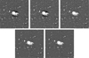 |
Fig. 1 Illustration of the main preprocessing steps on a g band image cutout. Top-left: original full-resolution image. Top-center: image after the 4 ×4 pixel binning. Top-right: corrected for background oversubtraction near bright objects (spiral galaxy at the center) and set anomalies, such as vertical stripes, to zero. Bottom-left: small objects replaced with nearby background noise. Bottom-right: MW stars replaced with the local background. |
3.2 Detections with MTObjects
MTOBJECTS (Max-Tree Objects; henceforth MTO) (Teeninga et al. 2015, 2016) is a detection software similar to SEP or SOURCE-EXTRACTOR, designed for the study of LSB objects. In contrast to SEP, which estimates and subtracts the local background, MTO calculates a global background value from areas devoid of objects and removes it. In SEP, a fixed thresh-old is chosen (an integer multiple of the standard deviation of the local background level) to differentiate between objects and background. In MTO, on the other hand, a so-called max-tree is constructed, which is a hierarchical representation of the image. The leaf nodes represent the image maxima, and parent nodes are progressively fainter regions of a given object. In a series of statistical tests using the estimated global background level and local node characteristics, the algorithm decides between real objects and noise. Compared to SEP, MTO excels at detecting LSB objects and correctly captures the faint outskirts of extended galaxies. It is also better at identifying nested objects and its background estimation is not biased by large objects in the image.
We used a Python implementation of MTO6 in our pipeline. We left default values for all but one parameter. The so-called “move factor” controls how many faint pixels are included in the outskirts of an object. With a lower value, we extend object boundaries to faint outer regions but also risk including noise. Since we are particularly interested in capturing LSB features, we moved this parameter from the default value of 0.5–0.39. We found this final value by trial and error, focusing on striking a balance between capturing most of the LSB outskirts of the objects and avoiding object blending. Since we chose a lower value for the move factor, it was necessary to carry out a careful preprocessing, such as removing small sources beforehand, to avoid including neighboring sources that were not physically connected to the object of interest. It was important to obtain real object boundaries as well as possible, so that MTO would be able to accurately calculate the structural parameters for the objects that were then used to filter the detections and select likely LSB candidates. We used SEP rather than MTO to detect point-like objects that should be masked in the preprocessing step because it is significantly faster and better at deblending point sources.
3.3 Postprocessing
After running MTO on the preprocessed image tiles, we used the output parameter file to derive structural parameters for all objects in arcseconds. By default the MTO implementation calculates the effective radius, Re, the radius at full-width-half-max of the light distribution, Rfwhm, and the radii at which 10 (R10) and 90 (R90) percent of the total light is emitted. It is important to note that these radius calculations are based on a simplified approach, where the pixels belonging to an object are sorted based on their brightness values (rather than their spatial distribution). The calculation does not consider the distance of pixels from the object’s center. Instead, it determines how many of the brightest pixels contribute to specific percentages of the total flux and then converts these pixel counts to equivalent circular radii using the formula ![Mathematical equation: $[r = \sqrt \frame{\frame{\text{~}}area\frame{\text{~}}/\pi } \]$](/articles/aa/full_html/2025/07/aa54501-25/aa54501-25-eq1.png) , effectively assuming a circular profile. The parameter Rfwhm is calculated as the radius of a circle that would contain all pixels that are at least half as bright as the brightest pixel in the distribution. On the other hand, Re is the radius of a circle containing the brightest pixels that together account for 50% of the total flux in the segment. After the initial experimentation using a binary random forest classifier to distinguish between dwarf galaxies and everything else, we analyzed the feature importance scores of the model. This analysis revealed that the radius parameters (in particular R10) had the highest significance with respect to these values, with the largest contribution to the classifier’s ability to discriminate between dwarf and non-dwarf objects. Therefore, we decided to add calculations for R25, R75, and R100 to the MTO source code. Then, R100 represents the radius of a circle with an area equivalent to the total area of all pixels assigned to an object by MTO. We initially applied a coarse filter to the MTO detections based on Re > 1.6 arcsec and a mean effective surface brightness of < μ >e > 19 mag/arcsec2. We removed possible satellite streaks by requiring an object axis ratio >0.17 for large detections, which is based on a set of streaks in the image tiles. This initial filter leaves about 400–600 candidates for every image tile.
, effectively assuming a circular profile. The parameter Rfwhm is calculated as the radius of a circle that would contain all pixels that are at least half as bright as the brightest pixel in the distribution. On the other hand, Re is the radius of a circle containing the brightest pixels that together account for 50% of the total flux in the segment. After the initial experimentation using a binary random forest classifier to distinguish between dwarf galaxies and everything else, we analyzed the feature importance scores of the model. This analysis revealed that the radius parameters (in particular R10) had the highest significance with respect to these values, with the largest contribution to the classifier’s ability to discriminate between dwarf and non-dwarf objects. Therefore, we decided to add calculations for R25, R75, and R100 to the MTO source code. Then, R100 represents the radius of a circle with an area equivalent to the total area of all pixels assigned to an object by MTO. We initially applied a coarse filter to the MTO detections based on Re > 1.6 arcsec and a mean effective surface brightness of < μ >e > 19 mag/arcsec2. We removed possible satellite streaks by requiring an object axis ratio >0.17 for large detections, which is based on a set of streaks in the image tiles. This initial filter leaves about 400–600 candidates for every image tile.
In the next step, we added labels to the detected candidates by cross-matching their positions with a catalog of known dwarfs we compiled from the literature. The catalog contains dwarfs from different surveys namely, ELVES (Carlsten et al. 2022), MATLAS (Duc et al. 2015; Bílek et al. 2020; Habas et al. 2020; Poulain et al. 2021), SAGA (Geha et al. 2017; Mao et al. 2021, 2024), SMUDGES (Zaritsky et al. 2019; Goto et al. 2023; Zaritsky et al. 2023), UDGs detected in the field around M101 (Merritt et al. 2014), and early-type dwarfs that were visually identified and presented in Paudel et al. (2023) using the DESI Legacy Imaging Surveys (Dey et al. 2019). Table 1 details (for each source catalog) the number of objects that fall within the UNIONS footprint and their corresponding measured or estimated distance ranges. For every match, we added the literature ID of the known dwarf galaxy and a dwarf label to the filtered MTO detection catalog. This catalog of known dwarf galaxies serves as the foundation for the training dataset we later used to finetune our machine learning classifier, as described in Section 3.4.
To further refine our selection and minimize false positives, we sought a clear separation between dwarf candidates and likely non-dwarfs. To achieve this, we gathered detections from all image tiles containing known dwarfs. Then, for each known dwarf, we selected the 20 nearest candidates as non-dwarf examples. We acknowledge that our assumption that candidates closest to known dwarfs from the literature are likely non-dwarfs – and would have been classified as such in previous surveys – has certain limitations. Our data may be deeper and of higher quality than that of previous surveys, potentially revealing dwarf galaxies that were previously undetectable. Nevertheless, this approach provided a reasonable initial approximation that we can use to establish a working filter. For every band individually, we created a series of plots between every combination of two derived object parameters, as well as some other derived products, such as the ratios between two parameters. For the g and r bands, we found the clearest separation between dwarf and non-dwarf in the mean effective surface brightness, < μ >e versus the apparent magnitude, m, plane. In the i band, the separation is less clear in this plane but is more apparent by plotting ratios between radius parameters versus the magnitude. In particular, R90/R75 vs. mi offers the clearest separation in i. With these filters, we estimate to remove ∼32%, 42%, and 28% of the non-dwarfs from the catalog of possible dwarf candidates for the g, r, and i bands, respectively. We would have also respectively removed ∼1.3%, 1.2%, and 1.5% of the real dwarfs, but left them in the catalog since they are validated in the literature and the calculated MTO structural parameters can be faulty due to any overlapping sources or possible errors during object segmentation. We provide the exact filtering criteria and parameter values used for this process in Appendix B.
After filtering the list of candidates for every band, we cross-matched the remaining detections using a coordinate matching approach. We first compiled all objects detected across the three bands, then identified potential matches within 10 arcsec of each other and built connected components using a union-find algorithm, which efficiently groups all related detections (if object A matches B and B matches C, all three are grouped). Generally, we required objects to be present in at least two bands, which eliminated many false positives such as residual light from stellar halos, corrupt data patches that are particular to one band, or MTO segmentation errors. However, we implemented an exception for known dwarf galaxies from the literature catalogs: these were retained even if detected in only one band, provided that at least two bands had valid data overall. In total, 48 of the dwarfs from the literature were only detected in a single band. We added this exception because some confirmed low-surface-brightness dwarfs might only be detectable in the r band, which is optimized for LSB science and probes to deeper surface brightnesses. Furthermore, even though an object may not be detectable by MTO in some of the bands, the machine learning classifier we used later on may still be able to extract useful information from the image. If an object passed our matching criteria, we created a 256 ×256 pixel cutout around the object coordinates from the first band the candidate is detected in and stacked the cutouts of the three bands. This way, the objects are aligned precisely, which is crucial for the following classification step. This cross-matching filter left on average ∼90 candidates for each image tile. Overall, 16 519 tiles have been observed in g, r, and i, which results in approximately 1.5 million candidates, out of which 2009 are dwarf galaxies following the sources from the literature noted above.
Number of dwarf galaxy candidates within the UNIONS footprint and their distance ranges, compiled from the listed literature catalogs.
3.4 Dwarf labeling and classification with Galaxy Zoo
Initial feature-based binary classification tests using random forests and gradient-boosted decision trees (eXtreme Gradient Boosting; XGBoost) on the MTO object parameters revealed that we would expect about 5% false positive and false negative predictions. This would result in about 160k positive predictions that need to be cleaned visually. This seemed like an unfeasible task and, therefore, we attempted a different approach. As demonstrated in Tanoglidis et al. (2021b), image-based deep learning models can lead to a significant performance boost over feature-based approaches for this particular task. Thus, we decided to finetune a deep neural network trained on a large database of annotated galaxy images.
We initially used a set of known dwarf galaxies and their nearest unclassified candidates as positive and negative examples, respectively, to finetune the deep learning model ZOOBOT7 (Walmsley et al. 2023). Rather than training the model from scratch, we adopted a finetuning approach given our limited number of positive labels (i.e., dwarf galaxies). ZOOBOT was originally trained on galaxy morphology classification tasks using data from the Dark Energy Survey (DES, Abbott et al. 2018), which benefited from millions of images labeled by Galaxy Zoo volunteers. Consequently, the pretrained weights already capture a robust representation of astronomical data, making ZOOBOT well suited for adaptation to our dwarf classification problem.
Initial tests revealed that the image-based model did not significantly outperform our previous feature-based one, with both methods showing a false-positive rate of ∼5%. Visual inspection of the training data showed significant label noise. Some “dwarf galaxies” from the literature were non-dwarfs, such as artifacts, cirrus, or diffuse light around bright stars, objects that could mislead automatic detection pipelines. Conversely, we found that some of the candidates we had initially assumed to be non-dwarfs (based on their proximity to known dwarfs from the literature) were actually good dwarf candidates that had been missed in previous surveys. This further confirmed the limitations of our initial assumption and highlighted the need for careful visual classification. To address these issues, we under-took a comprehensive relabeling of our training data, visually classifying both literature dwarfs and their nearest neighbors to establish reliable positive and negative examples.
For the visual classification, we used the original full-resolution image tiles, rather than the binned versions used in MTO detection, as the lower resolution can obscure important morphological features, causing background spiral galaxies to appear as featureless, dwarf-like objects. We created 256 × 256 pixel cutouts centered on each object and processed them through several steps to create RGB color images. First, we computed the intensity, I, as the average of the three bands. When data in one band was missing or corrupted, we synthesized the missing band by averaging the remaining two bands, ensuring we maintained the three-band image required by ZOOBOT. In the final RGB composition, we mapped the longest wavelength to the red channel, the intermediate to green, and the shortest to blue. We then applied an inverse hyperbolic sine stretch to each channel via
![Mathematical equation: $[channel\frame{~_\frame{\frame{\text{scaled~}}}} = \frame{\text{~}}channel\frame{\text{~}} \times \frac{\frame{arcsinh\left(\nolbrace \frame{\frac{\frame{Q \cdot I}}{\frame{\frame{\text{~}}stretch\frame{\text{~}}}}} \norbrace\right)}}{\frame{Q \cdot I}}.\]$](/articles/aa/full_html/2025/07/aa54501-25/aa54501-25-eq2.png) (1)
(1)
This equation is based on the work of Lupton et al. (2004), where Q is a softening parameter that controls the relative scale between linear and logarithmic behavior of the function. The stretch factor determines the intensity at which the logarithmic compression becomes significant. This scaling allows for a simultaneous visualization of faint LSB features and bright objects such as stars. Next, we applied gamma correction to each scaled band to enhance the perceived brightness of the final image. Given that the pixel distribution after scaling the channels includes negative values, we applied the gamma correction in a sign-preserving way, expressed as
![Mathematical equation: $[channel~ = sign(channel\frame{\text{~}}) \times \frame{\text{~}}\left|\nolbrace \frame{channel} \norbrace\right|\frame{\frame{\text{~}}^\gamma }\frame{\text{.~}}\]$](/articles/aa/full_html/2025/07/aa54501-25/aa54501-25-eq3.png) (2)
(2)
This step pushes positive and negative values apart, turning an approximately Gaussian distribution before gamma correction, to a bimodal one after, as illustrated in Figure 2. After extensive testing, we found optimal visual results with Q = 7, stretch = 125, and γ = 0.25. Finally, we stacked the scaled and gamma-corrected channels to create RGB images.
Four of our team members independently classified the 2009 dwarf candidates from the literature. Given the challenging nature of dwarf galaxy classification due to their diverse sizes, morphological types, and distances, we implemented a three-tier classification system: “yes” (1), “no” (0), and “unsure” (0.5). This system accommodates ambiguous cases, such as dwarf irregulars that can be difficult to distinguish from more massive late-type galaxies at greater distances. For example, candidates showing irregular features with hints of spiral structure were typically assigned to the “unsure” category. We performed visual classification by inspecting six different cutout versions for a given object in a grid: the full resolution 256 × 256 pixel RGB image cutout, a 2 × 2 binned version, a version that was first binned 2 × 2 and then smoothed with a Gaussian kernel8, the 2 × 2 binned r band cutout and two RGB cutout versions from the Legacy Survey (Dey et al. 2019). The first of these two is a 512 × 512 pixel image cutout downloaded from data release 10 of the Legacy Surveys as it appears on the Legacy Survey Sky Viewer9. The second is a 2 × 2 binned and enhanced version of the first cutout, using contrast-limited adaptive histogram equalization (CLAHE) to better visualize the LSB features. After the initial testing, we found that classifying an object based on a single RGB image cutout is not ideal when inspecting a large number of objects in quick succession that have vastly different properties, from bright and star-forming to extremely faint and LSB, due to the limited speed at which our eyes can adjust. We picked different degrees of binning and smoothing to aid in visualizing extremely faint and diffuse objects. The r band cutout further promotes the visibility of particularly diffuse objects due to its LSB optimization. Such objects might not be discernible in the stacked RGB image due to the local background removal in the other two bands. The Legacy Survey images were chosen significantly larger than the UNIONS cutouts to provide critical context in the case of large or interacting objects. We used a classification tool10 specifically developed for this task to label our training data. A snapshot of the tool’s user interface is shown in Figure C.1 in Appendix C.
To account for both inter-rater variation (different experts classifying the same image differently) and intra-rater variation (the same expert assigning different classifications to the same image across multiple viewings), each of the four raters classified every candidate three times. The final classification for each candidate was derived by averaging all 12 resulting labels. This average represents the probability that a given object is a dwarf galaxy. We can utilize this information to train our model and teach it to reproduce expert uncertainty when classifying objects. After visual classification, 1998 out of 2009 objects had a non-zero averaged label (indicating potential dwarfs), leaving 11 with a zero label (indicating unanimous non-dwarfs). Then, 4 out of these 11 were already flagged after visual inspection in the SMUDGES survey (Zaritsky et al. 2019; Goto et al. 2023; Zaritsky et al. 2023); for reference, we show the remaining 7 objects we visually classified as non-dwarfs in Appendix D. To balance the training dataset, we had to add more negative examples. Thus, two team members independently classified the same set of additional candidates, which were drawn from the pool of objects nearest to known dwarf galaxies. We took samples from this pool because we had initially hypothesized that these were the best candidates for non-dwarfs as they had likely already been inspected in other surveys and not classified as dwarfs (see Section 3.3). We continued classifying these candidates until we had enough agreed-upon non-dwarf objects (both raters assigned a zero label) to achieve a dataset with an overall mean label of 0.5. The final training dataset includes 1998 non-zero labels and 1465 zero labels. We show the distribution of these labels in Figure 3 and highlight the labeled literature dwarfs versus classified non-dwarfs in the UNIONS data. We applied the same RGB transformation to the training dataset as we did for visual classification.
To ensure robust model development and evaluation, the full dataset of labeled examples (see Figure 3) was first partitioned. We reserved 10% of the data as a stratified, held-out test set, which was not used during any model training or hyper-parameter optimization. The remaining 90% constituted the training-validation pool. The hyperparameters for the ZOOBOT model were optimized using this training-validation pool.
Following hyperparameter selection, an ensemble of ten ZOOBOT models was constructed to provide the final dwarf galaxy classifications. To build this ensemble and maximize the use of our labeled data for training the individual models, the training-validation pool was first divided into 10 equally sized, stratified segments, so-called folds. We then trained ten distinct ZOOBOT models. For the training of each of these models, one unique segment (representing 10% of the training-validation pool) was set aside as a validation set, used to monitor its training. The remaining nine segments (constituting 90% of the training-validation pool) were combined and used as the training data for that particular model. This procedure was repeated ten times, with each of the ten segments systematically serving as the validation set exactly once. This approach ensures that every data point within the training-validation pool contributed to the training process across nine of the models and was used for validation in one, thereby effectively utilizing the entire pool for developing the ensemble members, rather than reserving a fixed portion solely for validation. The final probability assigned to a candidate is the average of the predictions from the ten trained models. The overall performance of this ensemble was evaluated on the initially reserved test set.
Our chosen architecture is the ConvNeXT-Nano variant of ZOOBOT, based on the ConvNeXt architecture (Liu et al. 2022). For our application, we used the “FinetuneableZoobotClassifier” class with two classes but instead of rounding our mean classifications to be binary (dwarf or no dwarf), we introduced them to the model as so-called soft labels that take discrete values between 0 and 1, representing the probability pdwarf that a given object is a dwarf galaxy. We framed the problem such that the model predicts the probability distribution [1-pdwarf , pdwarf ]. The model outputs two logits that, after applying the Softmax function, can be interpreted as the probability distributions [1-ppred, ppred]. We used the Kullback–Leibler (KL) divergence as our loss function,
![Mathematical equation: $[\frame{L_\frame{K\frame{L_\frame{Div}}}} = \frame{y_\frame{\frame{\text{true~}}}} \cdot \log \left(\nolbrace \frame{\frac{\frame{\frame{y_\frame{\frame{\text{true~}}}}}}{\frame{\frame{y_\frame{\frame{\text{pred~}}}}}}} \norbrace\right) + \left(\nolbrace \frame{1 - \frame{y_\frame{\frame{\text{true~}}}}} \norbrace\right) \cdot \log \left(\nolbrace \frame{\frac{\frame{1 - \frame{y_\frame{\frame{\text{true~}}}}}}{\frame{1 - \frame{y_\frame{\frame{\text{pred~}}}}}}} \norbrace\right),\]$](/articles/aa/full_html/2025/07/aa54501-25/aa54501-25-eq4.png) (3)
(3)
where ytrue is our soft label and ypred the model prediction. This function measures the difference between the labeled and predicted probability distributions.
ZOOBOT is divided into five layer blocks. Earlier blocks generally learn simple features such as the overall shape of the galaxy, while later blocks, towards the output layer, learn increasingly complex and task-specific features. We therefore used a base learning rate for the last block and classification head, we then decreased this learning rate by 25% for each earlier block. With this, we made sure to utilize the pretrained model’s ability to extract general features and gave it more flexibility to adjust to more complex ones, specific to our task and dataset.
Even though we finetuned earlier blocks with low learning rates, our small set of labeled data compared to the number of model parameters quickly led to overfitting. To mitigate this effect, we applied data augmentations, including random rotations (an integer multiple of 90 degrees), random vertical and horizontal flips, random small variations in contrast and brightness, and the addition of noise. As mentioned earlier in this work, the data follow a bimodal distribution due to the gamma correction. We estimated the noise level in our images by taking ten random image tiles, creating a final segmentation map for each image tile by fusing the individual segmentation maps of SOURCE EXTRACTOR and MTO. We considered any pixel assigned to an object by either detection software to be signal and all other pixels to be noise. As illustrated in Figure 2, the noise follows a similar distribution to the signal. We estimated the location and standard deviations of the two noise peaks using a Gaussian mixture model (GMM). During the training, we augmented the data with noise sampled from this bimodal distribution with a tunable noise scale parameter to avoid dominating the signal. We selected a noise scale of 0.3 as a hyperparameter, which means we added noise with a standard deviation of 0.3 times the estimated one.
As a way to additionally improve generalization and to prevent the model from being over-confident in its predictions, we introduced a so-called label smoothing (Szegedy et al. 2016). While label smoothing is conventionally applied to hard (e.g., one-hot encoded) labels, we deemed its application appropriate as our label generation process, despite producing soft probabilities, frequently results in “hard” 0 or 1 values at the extreme ends of the [0,1] scale. These extreme target values can promote model overconfidence. With a smoothing parameter of α = 0.01, this technique adjusts our labels by moving them slightly towards 0.5, according to the equation:
![Mathematical equation: $[label\frame{~_\frame{smooth~}} = \frame{\text{~}}label\frame{\text{~}} \cdot (1 - \alpha ) + 0.5 \cdot \alpha .\]$](/articles/aa/full_html/2025/07/aa54501-25/aa54501-25-eq5.png) (4)
(4)
This modification of the target labels helps to mitigate the strong pull of the original “hard” 0 and 1 values and encourages the model to generate less extreme probability outputs.
We trained with a batch size of 128, using it as an additional regularization strategy and the ADAMW optimizer (Kingma & Ba 2014; Loshchilov & Hutter 2019), with an initial learning rate of 5 × 10⁻⁵, a weight decay factor of 0.05, and the so-called ReduceLROnPlateau scheduler. This scheduler dynamically reduces the learning rate during training if no improvement is achieved for a certain number of epochs. We reduced the learning rate by 25% if the training loss did not improve for five consecutive epochs. We trained until convergence, which took around 15 minutes for each of our 10 models on a single A100 GPU. The resulting model has approximately 15 × 106 parameters.
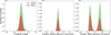 |
Fig. 2 Pixel value distribution in the r band for different stages of processing. Left: flux distribution in the original image tile. Middle: data after scaling via the inverse hyperbolic sine function. Right: bimodal distribution of the scaled data after gamma correction. Pixel values attributed to the signal (astronomical objects) are shown in green and the ones coming from areas devoid of objects (background noise) are shown in red. |
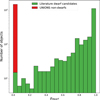 |
Fig. 3 Stacked histogram showing the label distribution in the dataset used for training. Dwarf candidates from the literature are shown in green, and non-dwarf objects are in red. The y-axis is shown on a logarithmic scale. |
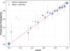 |
Fig. 4 Prediction vs label performance of the network on the test set consisting of 347 objects. On the x-axis, we show the 21 soft labels from our visual classification. On the y-axis, we show the mean predictions of the model in the 21 soft-label bins. The data point size reflects the number of examples in each bin, with the smallest points (e.g., two points between 0.1 and 0.2), representing bins containing only a single data point. Error bars represent the standard deviation of predictions within each bin. We assumed a Gaussian distribution to compute the mean and standard deviation. The red dashed line shows the one-to-one relation, indicating ideal calibration. |
4 Results
4.1 Model performance
Our models reached their lowest validation loss on average after 30 epochs and we used this ensemble of models for all fur- ther analyses. Figure 4 illustrates the performance of the model ensemble on the test set. The final predictions are calculated as the average prediction of our ten models. For simplicity, we are henceforth referring to our ensemble of models as one model. The model demonstrates generally robust performance across the soft label range, achieving a Brier score (Brier 1950) of BS = 0.0076. The Brier score ranges from 0 to 1, with 0 indicating perfect prediction and higher values indicating worse performance. For soft labels such as ours, which range between 0 and 1, this low score indicates that our model’s probabilistic predictions align well with our assigned probabilities. The Brier score, mathematically equivalent to the mean squared error between predicted and labeled probabilities, not only reflects overall prediction accuracy but also serves as a measure of the calibration quality between labels and predictions. To further quantify this calibration, the model achieves an expected calibration error (ECE) of 0.018. The ECE, ranging from 0 for perfect calibration to 1, represents the weighted average of the absolute difference between the average model-predicted probability and the average value of the corresponding soft labels within each probability bin. An ECE of 0.018 signifies that this weighted average deviation is 1.8 percentage points. This low ECE, much like the Brier score, indicates that the model’s confidence levels are well-aligned with the assigned soft label probabilities. The model shows a slight systematic under-confidence for objects with labels ≥ 0.8 and has the lowest level of confidence for labels in the range of roughly 0.05 to 0.5. This is unsurprising since few objects fall into this range in the training data (see Figure 3). In Figure 5, we illustrate the distribution of predicted probabilities color-coded by their labeled probability in bins covering intervals of 0.25 between 0 and 1. We see a clear progression of the four different probability distributions, where their spread shows the level of accuracy in predicting objects of a given category. In Figure 6, we show a gallery of five random example predictions on the test dataset in ten equally sized bins from 0 to 1. The column the object appears in indicates the probability bin assigned by the model and under every image cutout, we note the object’s soft label from our visual classification. We note a clear probability trend with predictions >0.8 showing good examples of dwarf galaxies and examples in the lowest bin showing clear non-dwarfs, such as distant massive galaxies.
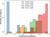 |
Fig. 5 Probability distribution of model predictions on the test dataset, color-coded by labels in four bins. The thickness of each bin distribution illustrates the level of accuracy in classifying objects of a given category. We note that the peaks of the distribution are distinct and show a consistent progression. |
4.2 The GOBLIN catalog
Using the trained model, we ran inference on all ( ∼1.5 million) MTO candidates that passed the filtering and band cross-matching step described in Section 3.3. Due to the tiling architecture of the UNIONS footprint, there is a slight overlap (∼ 3% total) between neighboring image tiles. Therefore, we removed any duplicate detections stemming from this overlap and from extended sources featuring regions of strongly varying brightness that may have been detected as two or more distinct objects. To achieve this efficiently, we use a friends-of-friends (FoF) clustering approach with a union-find algorithm to group objects that are close in angular separation. We used the object’s mean Re in the available bands as estimated by MTO to determine whether they are in the same group. Two objects are considered part of the same group if the angular separation between them is smaller than 1.5 times the effective radius of the larger object. We chose this factor to account for errors in the estimation of Re. We kept only the object with the highest model prediction from each group. This procedure removed ∼56k objects from the catalog, where ∼55k of the duplicates are due to the overlapping nature of the footprint and ∼1k are same-tile duplicates, mostly due to multiple detections of the same extended object.
We show the distribution of the model predictions on the de-duplicated catalog in Figure 7. Table 2 shows the corresponding detailed number of predictions in probability bins of 0.05. We note the stark difference between the populations in the first (0–0.05) and second (0.05–0.1) bins, illustrating that the vast majority ( ∼80%) of MTO candidates are non-dwarfs with a high confidence. Our catalog includes 42 965 objects with a model prediction score >0.8. We report this number because our visual inspection of the test set (see Figure 6) suggests that objects in these highest probability bins are consistently good dwarf candidates. However, this 0.8 threshold serves merely as a reference point, as the full catalog contains objects across the entire probability range, and many genuine dwarf galaxies likely exist at lower probability scores. Users of the GOBLIN catalog may select different thresholds depending on their specific requirements for completeness versus contamination. After removing objects that were in the training data, 41 462 candidates remain, with probabilities of >0.8.
In Figure 8, we show a 2D density map of all objects in the catalog with a model prediction >0.9 (23 072). We overlay the distribution of massive galaxies up to 120 Mpc and a stellar mass log (M∗ /M⊙) ≥10 that fall within the footprint. We gather the information about nearby massive galaxies from the Heraklion Extragalactic CATaloguE (HECATE; Kovlakas et al. 2021), a value-added catalog of galaxies up to a distance of 200 Mpc from the Milky Way. As expected, we see that peaks in the density map coincide with the presence of massive host galaxies. Blank regions within the footprint have not yet been covered by the three bands we used in this work.
It is important to note that while this spatial correlation provides circumstantial evidence supporting many of our candidates, our catalog has a fundamental limitation: we lack distance measurements for the vast majority of these objects. Even galaxies with high probability scores should still be considered candidates, as background spiral galaxies at larger distances can appear morphologically similar to nearby dwarf galaxies when their detailed features (such as spiral arms) become unresolvable due to distance. The angular resolution limits of our observations mean that distant galaxies lose their distinctive morphological characteristics and may be classified as dwarf-like based on their apparent size, surface brightness, and diffuse appearance. Therefore, although the correlation with massive galaxies is encouraging, individual confirmation of these candidates requires dedicated follow-up observations.
We present a small sample of our extensive GOBLIN catalog in Table 3. The full version is available at the CDS. The catalog contains the object’s coordinates right ascension and declination in degrees, the literature ID if it is in one of the dwarf catalogs we used for training, a column indicating whether or not the object was used to train our model, its soft label from our visual classification, the UNIONS tile it appears in, the model prediction and several photometric parameters provided by MTO and derived properties (e.g., magnitude and mean effective surface brightness). We provide these parameters in g, r, and i. If a given object was not detected in one of the bands, the corresponding columns are filled with NaN values. We note that these MTO parameters were derived from the binned images. The magnitudes and, therefore, the mean effective surface brightnesses are calculated by multiplying the total flux measured on the binned image tiles by a factor of 16 to account for the 4 × 4 binning scheme. They should not be regarded as accurate measurements but rather as rough estimates. To gain accurate structural parameters, a 2D model fitting via software such as GALFIT (Peng et al. 2010) should be used.
To illustrate and quantify the quality of the parameters obtained through MTO, we gathered photometric measurements for the dwarf galaxies from the literature that we used to train our model. Different parameters are available for the source catalogs we used. We gathered the effective radius, the magnitude, as well as the mean effective surface brightness in the g band and r band, where available. We show parameter comparisons between MTO and literature measurements in Figures E.1 and E.2 in Appendix E. We note that MTO largely underestimates the effective radius, in particular, towards larger values and for objects from the SMUDGES survey (Zaritsky et al. 2019, 2023; Goto et al. 2023). This discrepancy is caused by the method by which MTO calculates the effective radius (see Section 3.3). The magnitudes are approximately consistent, albeit with a positive bias for the g band and a scaling bias for the r band. We can correct for these biases by fitting linear relationships to the data. The standard deviations of the residuals for these linear fits are σres(g) = 0.59 and σres(r) = 0.42. In the final catalog, we report the measured magnitudes as well as the corrected relationships for the g and r bands. There are no corresponding i band measurements available in the literature. As a consequence of the discrepancy in the effective radius measurement, the mean effective surface brightness ends up largely underestimated by MTO. We did not attempt to correct the effective radius and the mean effective surface brightness since the discrepancy cannot be accounted for by a simple linear shift.
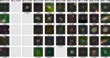 |
Fig. 6 Gallery of multiple different cutout examples from the test dataset. The columns are divided into prediction probability bins from the network. Under every cutout, we show the soft label from our visual classification. Gray squares indicate missing examples in a given probability bin. |
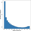 |
Fig. 7 Probability distribution of model predictions of the full deduplicated catalog of MTO candidates. The y-axis is shown on a logarithmic scale. |
Distribution of objects across the different probability bins.
5 Summary and conclusions
In this work, we have conducted an extensive search for dwarf galaxies in the UNIONS footprint, a deep and wide optical survey in the northern hemisphere. We have developed an automatic method to robustly detect these objects in an elaborate multi-step process that heavily relies on image preprocessing and uses machine learning in the final classification step. We ran our pipeline on all UNIONS tiles that have been observed and reduced in the g, r, and i bands at the time of writing. These bands are most relevant for detecting LSB objects, cover most of the final UNIONS footprint and exhibit a good overlap. For each band, there are ∼20k 0.51 × 0.51 deg image tiles available, and ∼16.5k are covered by all three. After a preprocessing routine that involves binning the image, along with detecting and masking corrupted data patches, small sources, and stars, we employed the software MTO to detect LSB objects. We filtered the resulting detections by making parameter cuts using known dwarfs from the literature that reside in the UNIONS footprint. Cross-matching the detections between the three bands and requiring a detection to be present in at least two out of three bands led to the final catalog of candidates (∼90 detections per tile).
We finetuned the deep-learning model ZOOBOT, which was pretrained on galaxy morphology classification tasks using labeled data from the Galaxy Zoo project. After initial attempts using dwarf galaxies from various catalogs from the literature yielded poor results, we relabeled ∼2000 literature dwarfs plus ∼1500 non-dwarf examples from the UNIONS data. The average of these labels represents the probability that a given object is a dwarf galaxy. We used this information to train our dwarf galaxy classifier, and rather than outputting a binary classification (dwarf or no dwarf), the model learned to predict the probability that an object is a dwarf.
We applied the trained model on the ∼1.5 × 10⁶ candidates and, thus, we assigned a dwarf probability to each of them. After removing duplicate detections due to the small overlap between neighboring tiles and large objects being split into multiple detections, 1 478 733 objects remain in the catalog. Following our model predictions, the vast majority (∼ 80%) of these objects are non-dwarfs (pmodel < 0.05). Finally, 42 965 objects achieved a probability of >0.8 and 41 462 of these were not used to train the model.
A density map of the highest probability candidates reveals that the detected objects follow the projected distribution of massive galaxies in the sky. In a future work, we will conduct a detailed study of the distribution of these identified objects in relation to their potential host galaxies.
While our detection approach has identified a vast number of dwarf galaxy candidates, we acknowledge that some of these objects may have been previously detected in other surveys. Given the distributed nature of astronomical databases and the continuous updates to the literature, we present this as an independent catalog rather than claiming first detections. We provide the complete de-duplicated catalog of ∼1.5 million objects along with their classification probabilities, allowing researchers to select candidates based on probability thresholds that best suit their specific science goals. Whether we are studying the most secure candidates (pmodel > 0.9) or investigating a larger sample with more relaxed probability cuts, the GOBLIN catalog’s flexible character supports a wide range of scientific investigations. We anticipate that this comprehensive dataset will serve as a valuable resource for the community, enabling various follow-up studies and complementing existing catalogs of LSB galaxies.
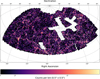 |
Fig. 8 Distribution of high-confidence dwarf galaxy candidates (prediction score >0.9) from the GOBLIN catalog on a Lambert azimuthal equalarea projection. Each pixel (or bin) represents an equal size of 0.5 × 0.5 degrees, regardless of the location on the map. Black dots with white outlines show massive galaxies up to 120 Mpc with stellar masses log (M∗/M⊙)≥ 10. The color bar shows counts per bin on a logarithmic scale. Colored areas show survey coverage in g, r, and i. |
Sample of the full GOBLIN catalog with a subset of the available columns.
Data availability
Full Table 3 is available at the CDS via anonymous ftp to cdsarc.cds.unistra.fr (130.79.128.5) or via https://cdsarc.cds.unistra.fr/viz-bin/cat/J/A+A/699/A232
Acknowledgements
We thank the referee for the constructive report, which helped to clarify and improve the manuscript. O.M. and N.H. are grateful to the Swiss National Science Foundation for financial support under the grant number PZ00P2_202104. N.H. thanks Stephen Gwyn for the help provided with questions regarding the UNIONS data. N.H. also thanks Jean-Charles Cuillandre for clarifying the nature of the surface brightness limit for the UNIONS r band data. E.S. is grateful to the Leverhulme Trust for funding under the grant number RPG-2021-205. D.C. is grateful for the financial support provided by the Harding Distinguished Postgraduate Scholars Programme. MJH acknowledges support from NSERC through a Discovery Grant. We are honored and grateful for the opportunity of observing the Universe from Maunakea and Haleakala, which both have cultural, historical and natural significance in Hawaii. This work is based on data obtained as part of the Canada-France Imaging Survey, a CFHT large program of the National Research Council of Canada and the French Centre National de la Recherche Scientifique. Based on observations obtained with MegaPrime/MegaCam, a joint project of CFHT and CEA Saclay, at the Canada-France-Hawaii Telescope (CFHT) which is operated by the National Research Council (NRC) of Canada, the Institut National des Science de l’Univers (INSU) of the Centre National de la Recherche Scientifique (CNRS) of France, and the University of Hawaii. This research used the facilities of the Canadian Astronomy Data Centre operated by the National Research Council of Canada with the support of the Canadian Space Agency. This research is based in part on data collected at Subaru Telescope, which is operated by the National Astronomical Observatory of Japan. Pan-STARRS is a project of the Institute for Astronomy of the University of Hawaii, and is supported by the NASA SSO Near Earth Observation Program under grants 80NSSC18K0971, NNX14AM74G, NNX12AR65G, NNX13AQ47G, NNX08AR22G, 80NSSC21K1572 and by the State of Hawaii. This work has made use of data from the European Space Agency (ESA) mission Gaia (https://www.cosmos.esa.int/gaia), processed by the Gaia Data Processing and Analysis Consortium (DPAC, https://www.cosmos.esa.int/web/gaia/dpac/consortium). Funding for the DPAC has been provided by national institutions, in particular the institutions participating in the Gaia Multilateral Agreement. This research made use of Photutils, an Astropy package for detection and photometry of astronomical sources (Bradley et al. 2024).
Appendix A Enhancing UDG detectability through binning
The 4 × 4 binning scheme we applied as our first preprocessing step of the original images is motivated by the detectability gains for some of the faintest objects we gathered from the literature. In Figure A.1 we illustrate this sensitivity enhancement by showing the full resolution images vs. binned images and the corresponding MTO segmentation maps.
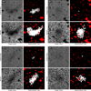 |
Fig. A.1 Detectability of four UDGs detected around NGC 5485 in Merritt et al. (2014) before and after 4 × 4 binning. Each quadrant presents one source with four panels arranged as follows: original data (upper left) with its corresponding segmentation map (upper right), and 4 × 4 binned data (lower left) with its corresponding segmentation map (lower right). The segmentation map shows the UDG segment in white and all other sources in red. |
Appendix B Object filtering criteria
To identify potential dwarf galaxy candidates, we implemented a multi-stage filtering process across the three different photometric bands we used in this work. For each band, we applied both basic threshold filtering and complex relational criteria designed to isolate low-surface-brightness galaxies. Tables B.1, B.2, and B.3 present the basic selection thresholds applied to our catalog in the r, g, and i bands, respectively. Beyond basic thresholds, we implemented more complex relational criteria to refine our selection further. These criteria were empirically derived to maximize the inclusion of known dwarf galaxies from the literature while minimizing contamination from other astronomical sources. We report these relational criteria for each band in the following subsections. In addition to the parameters already described in Table 3, μmedian, μmean, μmax are the median, mean and maximum pixel values of the objects provided by MTO. Dashes in the tables indicate the absence of a limiting value. In Figure B.1 we show examples of separation criteria for the different bands that allowed for the clearest separations between dwarfs and likely non-dwarfs we could determine for our dataset.
B.1 Filtering criteria for the r band
Basic selection criteria for the r band
![Mathematical equation: $[\frame{\mu _r}\frame{ > _e}0.6155 \times \frame{m_r} + 10.2257,\]$](/articles/aa/full_html/2025/07/aa54501-25/aa54501-25-eq6.png) (B.1)
(B.1)
![Mathematical equation: $[\frame{\mu _r}\frame{ > _e}1.35 \times \frame{m_r} - 5.3464,\]$](/articles/aa/full_html/2025/07/aa54501-25/aa54501-25-eq7.png) (B.2)
(B.2)
![Mathematical equation: $[\frac{\frame{\frame{\mu _r}_e}}{\frame{\frame{R_\frame{75}}}} < \max \left(\nolbrace \frame{1.3611 \times \frame{m_r} - 18.2513,2.51} \norbrace\right),\]$](/articles/aa/full_html/2025/07/aa54501-25/aa54501-25-eq8.png) (B.3)
(B.3)
![Mathematical equation: $[\log \left(\nolbrace \frame{\frac{\frame{\frame{R_\frame{90}}}}{\frame{\frame{R_\frame{75}}}}} \norbrace\right) < 0.295 \times \log \left(\nolbrace \frame{\frame{R_\frame{100}}} \norbrace\right) - 0.13.\]$](/articles/aa/full_html/2025/07/aa54501-25/aa54501-25-eq9.png) (B.4)
(B.4)
Basic selection criteria for the WHIGS g band
B.2 Filtering criteria for the g band
![Mathematical equation: $[\frame{\mu _g}\frame{ > _e}0.7063 \times \frame{m_g} + 8.5579,\]$](/articles/aa/full_html/2025/07/aa54501-25/aa54501-25-eq10.png) (B.5)
(B.5)
![Mathematical equation: $[\frame{\mu _g}\frame{ > _e}4.1 \times \frame{m_g} - 68.6681\frame{\text{,~}}\]$](/articles/aa/full_html/2025/07/aa54501-25/aa54501-25-eq11.png) (B.6)
(B.6)
![Mathematical equation: $[\log \left(\nolbrace \frame{\frac{\frame{\frame{R_\frame{100}}}}{\frame{\frame{R_\frame{90}}}}} \norbrace\right) < - 1.0795 \times \log \left(\nolbrace \frame{\frame{m_g}} \norbrace\right) + 3.57,\]$](/articles/aa/full_html/2025/07/aa54501-25/aa54501-25-eq12.png) (B.7)
(B.7)
![Mathematical equation: $[\log \left(\nolbrace \frame{\frac{\frame{\frame{m_g}}}{\frame{\frame{R_\frame{75}}}}} \norbrace\right) < \max \left(\nolbrace \frame{5.6017 \times \log \left(\nolbrace \frame{\frame{m_g}} \norbrace\right) - 14.6037,0.57} \norbrace\right)\]$](/articles/aa/full_html/2025/07/aa54501-25/aa54501-25-eq13.png) (B.8)
(B.8)
B.3 Filtering criteria for the i band
Basic selection criteria for the i band
![Mathematical equation: $[\frac{\frame{\frame{R_\frame{90}}}}{\frame{\frame{R_\frame{75}}}} < 0.01 \times \frame{R_\frame{100}} + 1.4\]$](/articles/aa/full_html/2025/07/aa54501-25/aa54501-25-eq14.png) (B.9)
(B.9)
![Mathematical equation: $[\frac{{{R_{100}}}}{{{R_{90}}}} < - 0.085 \times {m_i} + 3.0441,\]$](/articles/aa/full_html/2025/07/aa54501-25/aa54501-25-eq15.png) (B.10)
(B.10)
![Mathematical equation: $[\frac{\frame{\frame{m_i}}}{\frame{\frame{R_\frame{75}}}} < \max \left(\nolbrace \frame{1.2479 \times \frame{m_i} - 16.9164,2.08} \norbrace\right),\]$](/articles/aa/full_html/2025/07/aa54501-25/aa54501-25-eq16.png) (B.11)
(B.11)
![Mathematical equation: $[\frac{{{R_{90}}}}{{{R_{75}}}} < - 0.07 \times {m_i} + 2.7593,\]$](/articles/aa/full_html/2025/07/aa54501-25/aa54501-25-eq17.png) (B.12)
(B.12)
![Mathematical equation: $[\frac{{{R_{75}}}}{{{R_{25}}}} < 0.2 \times {m_i} + 1.6021\]$](/articles/aa/full_html/2025/07/aa54501-25/aa54501-25-eq18.png) (B.13)
(B.13)
![Mathematical equation: $[\frac{{{R_{75}}}}{{{R_{25}}}} < - 1.1 \times {m_i} + 27.1887\]$](/articles/aa/full_html/2025/07/aa54501-25/aa54501-25-eq19.png) (B.14)
(B.14)
![Mathematical equation: $[\log \left(\nolbrace \frame{\frac{\frame{\frame{R_\frame{100}}}}{\frame{\frame{R_\frame{75}}}}} \norbrace\right) < - 2.3353 \times \log \left(\nolbrace \frame{\frame{m_i}} \norbrace\right) + 7.5703\]$](/articles/aa/full_html/2025/07/aa54501-25/aa54501-25-eq20.png) (B.15)
(B.15)
![Mathematical equation: $[\log \left(\nolbrace \frame{\frac{\frame{\frame{R_\frame{75}}}}{\frame{\frame{R_\frame{25}}}}} \norbrace\right) < 0.6606 \times \log \left(\nolbrace \frame{\frame{m_i}} \norbrace\right) - 0.2820.\]$](/articles/aa/full_html/2025/07/aa54501-25/aa54501-25-eq21.png) (B.16)
(B.16)
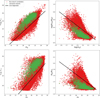 |
Fig. B.1 Examples of parameter spaces used to filter dwarf galaxy candidates. These four panels show the clearest separations we could empirically determine for our data between known dwarf galaxies from the literature (green points) and their nearest neighbors assumed to be non-dwarfs (red points). Top-left: Mean effective surface brightness, < μg >e vs. apparent magnitude, mg in the g band. Top-right: log(R100/R90) vs. log(mg) in the g band. Bottom-left: Mean effective surface brightness, < μr >e vs. mr in the r band. Bottom-right: R90/R75 vs. mi in the i band. The solid black line in each panel indicates the selection boundary we applied to filter out likely non-dwarf objects while preserving the majority of known dwarfs. The lines follow the relations B.5, B.7, B.1, and B.12, respectively. |
Appendix C Classification tool
In Figure C.1, we show the user interface (UI) for the classification tool we used to label our training data. It supports both single-view (single RGB cutout) and multi-view (six different versions of the same cutout) classification. The first question asks about the nature of the object, with the possible answers “dwarf” (1), “maybe dwarf” (0.5), and “no dwarf” (0). If the first question is answered with “dwarf” or “maybe dwarf”, the user is asked about the morphology of the candidate. The possible choices are dwarf elliptical (dE), nucleated dwarf elliptical (dEN), dwarf irregular (dI), and nucleated dwarf irregular (dIN). The third question asks about special features, such as globular clusters, or whether the object is disturbed due to gravitational interaction. In this work, we only utilized the answers to the first question about the dwarf nature, but we plan to use the additional classifications in future work.
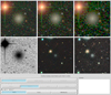 |
Fig. C.1 Classification tool used to label our training data. The UI shows six different views of the same object. Top-left: Full resolution RGB image cutout, top-center: 2 × 2 binned RGB cutout, top-right: 2 × 2 binned and smoothed RGB cutout. Bottom-left: r band image cutout. Bottom-center: Legacy Survey cutout. Bottom-right: 2 × 2 binned and CLAHE enhanced Legacy Survey cutout. The tool asks the questions: 1) Is this a dwarf galaxy? If yes or maybe: 2) What is the morphology? and 3) Any special feature? Finally, a comment box is available to note any additional features. |
Appendix D Visually classified non-dwarfs
During the visual classification of dwarf galaxies presented in the literature, we found 7 objects that we unanimously classified as non-dwarfs during all three classification runs. For reference, we show image cutouts of these objects along with their source catalog in Figure D.1.
 |
Fig. D.1 RGB image cutouts of objects we unanimously visually classified as non-dwarfs while generating labels to train our dwarf classifier. These objects were reported as dwarf galaxy candidates in the literature. We show their ID in the top left corner and the source catalog in the bottom right corner of every cutout. The references for the source papers are SMUDGES (Goto et al. 2023; Zaritsky et al. 2023) and dEs in the Local Universe (Paudel et al. 2023). |
Appendix E Comparison between MTO and literature parameters
This section compares MTO-derived parameters with published literature values for the dwarf galaxy candidates used in our training sample. In Figure E.1 we show the comparison for the effective radius, Re. We note that Re is mostly underestimated by MTO, especially towards larger radii. We attribute this discrepancy to the fact that MTO does not calculate Re via a radial profile, but sorts the pixels, regardless of their location from the center of the object, to calculate the effective radius. In Figure E.2 we show the comparisons for the absolute magnitude, m and the mean effective surface brightness, < μ >e in the g and r bands; corresponding i band parameters are not available in the literature sample. For the magnitudes, there is a positive bias for the g band, i.e., MTO systematically overestimates the magnitude. For the r band, there is a scaling bias, i.e., the data points follow a different slope than the one-to-one relation. These two biases can be corrected via simple linear shifts. Therefore, we report the corrected along with the measured values for mg and mr in the final catalog. The standard deviations of the residuals after this correction are σres(g) = 0.59 and σres(r) = 0.42. Due to the discrepancy in the determination of Re, < μ >e is also largely underestimated but cannot be addressed via a linear correction.
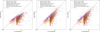 |
Fig. E.1 Comparison between the effective radii Re measured by MTO and the values reported in the literature for the dwarf candidates we used to train our model. We show the literature values on the x-axis and the values measured by MTO on the y-axis. Both axes are shown on logarithmic scales. The data points are color coded by the survey they were identified in as shown in the figure legends. The one-to-one relation is plotted as the gray dashed line. We compare our measurements in the individual bands with the single values reported in the literature. Left: g band, center: r band, and right: i band. |
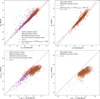 |
Fig. E.2 Comparison between the apparent magnitudes, m (top row) and the mean effective surface brightnesses, < μ >e (bottom row) derived from the MTO measurements and the values reported in the literature for the dwarf candidates we used to train our model. We show the literature values on the x-axis and the values measured by MTO on the y-axis. The data points are color coded by the survey they were identified in as shown in the figure legends. The one-to-one relation is plotted as the gray dashed line. The red dashed line in the top row plots shows a linear fit to the data that can be used to correct the magnitude offset from the one-to-one relation. We report the standard deviation of the residuals with respect to this linear fit σres in the legend. Left column: g band, right column: r band. |
References
- Abbott, T. M. C., Abdalla, F. B., Allam, S., et al. 2018, ApJS, 239, 18 [Google Scholar]
- Aihara, H., Arimoto, N., Armstrong, R., et al. 2018a, PASJ, 70, S4 [NASA ADS] [Google Scholar]
- Aihara, H., Armstrong, R., Bickerton, S., et al. 2018b, PASJ, 70, S8 [NASA ADS] [Google Scholar]
- Ayçoberry, E., Ajani, V., Guinot, A., et al. 2023, A&A, 671, A17 [NASA ADS] [CrossRef] [EDP Sciences] [Google Scholar]
- Babusiaux, C., Fabricius, C., Khanna, S., et al. 2023, A&A, 674, A32 [NASA ADS] [CrossRef] [EDP Sciences] [Google Scholar]
- Barbary, K. 2016, JOSS, 1, 58 [Google Scholar]
- Bennet, P., Sand, D. J., Crnojević, D., et al. 2017, ApJ, 850, 109 [NASA ADS] [CrossRef] [Google Scholar]
- Bennet, P., Sand, D., Crnojević, D., et al. 2020, ApJ, 893, L9 [CrossRef] [Google Scholar]
- Bertin, E. 2010, Astrophysics Source Code Library [record ascl:1010.068] [Google Scholar]
- Bertin, E., & Arnouts, S. 1996, A&AS, 117, 393 [NASA ADS] [CrossRef] [EDP Sciences] [Google Scholar]
- Bickley, R. W., Bottrell, C., Hani, M. H., et al. 2021, MNRAS, 504, 372 [NASA ADS] [CrossRef] [Google Scholar]
- Bickley, R. W., Ellison, S. L., Patton, D. R., et al. 2022, MNRAS, 514, 3294 [NASA ADS] [CrossRef] [Google Scholar]
- Bickley, R. W., Ellison, S. L., Patton, D. R., & Wilkinson, S. 2023, MNRAS, 519, 6149 [CrossRef] [Google Scholar]
- Bílek, M., Duc, P.-A., Cuillandre, J.-C., et al. 2020, MNRAS, 498, 2138 [Google Scholar]
- Binggeli, B., Sandage, A., & Tammann, G. A. 1985, AJ, 90, 1681 [Google Scholar]
- Binggeli, B., Tarenghi, M., & Sandage, A. 1990, A&A, 228, 42 [NASA ADS] [Google Scholar]
- Bom, C., Poh, J., Nord, B., Blanco-Valentin, M., & Dias, L. 2019, arXiv e-prints [arXiv:1911.06341] [Google Scholar]
- Bosch, J., Armstrong, R., Bickerton, S., et al. 2018, PASJ, 70, S5 [Google Scholar]
- Bosch, J., AlSayyad, Y., Armstrong, R., et al. 2019, in ASP Conference Series, 523, ADASS XXVII, eds. P. J. Teuben, M. W. Pound, B. A. Thomas, & E. M. Warner, 521 [Google Scholar]
- Bradley, L., Sipőcz, B., Robitaille, T., et al. 2024, 10.5281/zenodo.12585239 [Google Scholar]
- Brier, G. W. 1950, Monthly Weather Rev., 78, 1 [CrossRef] [Google Scholar]
- Bullock, J. S., & Boylan-Kolchin, M. 2017, ARA&A, 55, 343 [Google Scholar]
- Caldeira, J., Wu, W. K., Nord, B., et al. 2019, Astron. Comput., 28, 100307 [NASA ADS] [CrossRef] [Google Scholar]
- Carlsten, S. G., Beaton, R. L., Greco, J. P., & Greene, J. E. 2019, ApJ, 878, L16 [NASA ADS] [CrossRef] [Google Scholar]
- Carlsten, S. G., Greene, J. E., Beaton, R. L., Danieli, S., & Greco, J. P. 2022, ApJ, 933, 47 [CrossRef] [Google Scholar]
- Chambers, K. C., Magnier, E., Metcalfe, N., et al. 2016, arXiv e-prints [arXiv:1612.05560] [Google Scholar]
- Chan, J., Lemon, C., Courbin, F., et al. 2022, A&A, 659, A140 [NASA ADS] [CrossRef] [EDP Sciences] [Google Scholar]
- Cheng, T.-Y., Conselice, C. J., Aragón-Salamanca, A., et al. 2020, MNRAS, 493, 4209 [Google Scholar]
- Chiboucas, K., Jacobs, B. A., Tully, R. B., & Karachentsev, I. D. 2013, AJ, 146, 126 [Google Scholar]
- Chu, A., Durret, F., Ellien, A., et al. 2023, A&A, 673, A100 [NASA ADS] [CrossRef] [EDP Sciences] [Google Scholar]
- Ćiprijanović, A., Snyder, G. F., Nord, B., & Peek, J. E. 2020, Astron. Comput., 32, 100390 [NASA ADS] [CrossRef] [Google Scholar]
- Collins, M. L. M., Tollerud, E. J., Rich, R. M., et al. 2020, MNRAS, 491, 3496 [NASA ADS] [CrossRef] [Google Scholar]
- Cortes, C. & Vapnik, V. 1995, Mach. Learn., 20, 273 [Google Scholar]
- Crnojević, D., Sand, D., Bennet, P., et al. 2019, ApJ, 872, 80 [Google Scholar]
- Crosby, E., Jerjen, H., Müller, O., et al. 2023, MNRAS, 521, 4009 [Google Scholar]
- Crosby, E., Jerjen, H., Müller, O., et al. 2024, MNRAS, 527, 9118 [Google Scholar]
- Danieli, S., & van Dokkum, P. 2019, ApJ, 875, 155 [Google Scholar]
- Danieli, S., van Dokkum, P., Merritt, A., et al. 2017, ApJ, 837, 136 [NASA ADS] [CrossRef] [Google Scholar]
- Davies, A., Serjeant, S., & Bromley, J. M. 2019, MNRAS, 487, 5263 [NASA ADS] [CrossRef] [Google Scholar]
- De Angeli, F., Weiler, M., Montegriffo, P., et al. 2023, A&A, 674, A2 [NASA ADS] [CrossRef] [EDP Sciences] [Google Scholar]
- Dey, A., Schlegel, D. J., Lang, D., et al. 2019, AJ, 157, 168 [Google Scholar]
- Dieleman, S., Willett, K. W., & Dambre, J. 2015, MNRAS, 450, 1441 [NASA ADS] [CrossRef] [Google Scholar]
- Doliva-Dolinsky, A., Collins, M. L. M., & Martin, N. F. 2025, arXiv e-prints, [arXiv:2502.06948] [Google Scholar]
- Domber, J. L., Gygax, J. D., Aumiller, P., et al. 2022, SPIE Conf. Ser., 12180, 121801O [Google Scholar]
- Domínguez Sánchez, H., Huertas-Company, M., Bernardi, M., Tuccillo, D., & Fischer, J. 2018, MNRAS, 476, 3661 [CrossRef] [Google Scholar]
- Drlica-Wagner, A., Carlin, J. L., Nidever, D. L., et al. 2021, ApJS, 256, 2 [NASA ADS] [CrossRef] [Google Scholar]
- Drlica-Wagner, A., Ferguson, P. S., Adamów, M., et al. 2022, ApJS, 261, 38 [NASA ADS] [CrossRef] [Google Scholar]
- Duc, P.-A., Cuillandre, J.-C., Karabal, E., et al. 2015, MNRAS, 446, 120 [Google Scholar]
- Ellison, S. L., Viswanathan, A., Patton, D. R., et al. 2019, MNRAS, 487, 2491 [NASA ADS] [CrossRef] [Google Scholar]
- Ellison, S. L., Wilkinson, S., Woo, J., et al. 2022, MNRAS, 517, L92 [NASA ADS] [CrossRef] [Google Scholar]
- Euclid Collaboration (Mellier, Y., et al.) 2025, A&A, 697, A1 [Google Scholar]
- Fantin, N. J., Côté, P., McConnachie, A. W., et al. 2019, ApJ, 887, 148 [NASA ADS] [CrossRef] [Google Scholar]
- Fantin, N. J., Côté, P., McConnachie, A. W., et al. 2021, ApJ, 913, 30 [NASA ADS] [CrossRef] [Google Scholar]
- Ferguson, H. C. 1989, AJ, 98, 367 [Google Scholar]
- Ferguson, H. C., & Binggeli, B. 1994, A&A Rev., 6, 67 [NASA ADS] [CrossRef] [Google Scholar]
- Ferguson, A. M., Irwin, M. J., Ibata, R. A., Lewis, G. F., & Tanvir, N. R. 2002, AJ, 124, 1452 [Google Scholar]
- Ferguson, H. C., & Sandage, A. 1988, AJ, 96, 1520 [Google Scholar]
- Ferguson, H. C., & Sandage, A. 1990, AJ, 100, 1 [NASA ADS] [CrossRef] [Google Scholar]
- Ferrarese, L., Cote, P., Cuillandre, J.-C., et al. 2012, ApJS, 200, 4 [NASA ADS] [CrossRef] [Google Scholar]
- Ferreira, L., Bickley, R. W., Ellison, S. L., et al. 2024, MNRAS, 533, 2547 [NASA ADS] [CrossRef] [Google Scholar]
- Frenk, C. S., & White, S. D. 2012, Ann. Phys., 524, 507 [NASA ADS] [CrossRef] [Google Scholar]
- Gaia Collaboration (Prusti, T., et al.) 2016, A&A, 595, A1 [NASA ADS] [CrossRef] [EDP Sciences] [Google Scholar]
- Gaia Collaboration (Mignard, F., et al.) 2018, A&A, 616, A14 [NASA ADS] [CrossRef] [EDP Sciences] [Google Scholar]
- Gaia Collaboration (Vallenari, A., et al.) 2023, A&A, 674, A1 [NASA ADS] [CrossRef] [EDP Sciences] [Google Scholar]
- Geha, M., Wechsler, R. H., Mao, Y.-Y., et al. 2017, ApJ, 847, 4 [NASA ADS] [CrossRef] [Google Scholar]
- Goto, H., Zaritsky, D., Karunakaran, A., Donnerstein, R., & Sand, D. J. 2023, AJ, 166, 185 [Google Scholar]
- Greco, J. P., Greene, J. E., Strauss, M. A., et al. 2018, ApJ, 857, 104 [NASA ADS] [CrossRef] [Google Scholar]
- Guerrini, S., Kilbinger, M., Leterme, H., et al. 2024, A&A, submitted [arXiv:2412.14666] [Google Scholar]
- Guinot, A., Kilbinger, M., Farrens, S., et al. 2022, A&A, 666, A162 [NASA ADS] [CrossRef] [EDP Sciences] [Google Scholar]
- Gwyn, S. D. 2008, PASP, 120, 212 [Google Scholar]
- Gwyn, S. 2019, ADASS XXVII, 523, 649 [Google Scholar]
- Gwyn, S., McConnachie, A. W., Cuillandre, J.-C., et al. 2025, AJ, submitted [arXiv:2503.13783] [Google Scholar]
- Habas, R., Marleau, F. R., Duc, P.-A., et al. 2020, MNRAS, 491, 1901 [NASA ADS] [Google Scholar]
- Ibata, R. A., Gilmore, G., & Irwin, M. 1994, Nature, 370, 194 [NASA ADS] [CrossRef] [Google Scholar]
- Ibata, R., Martin, N. F., Irwin, M., et al. 2007, ApJ, 671, 1591 [CrossRef] [Google Scholar]
- Ibata, R. A., McConnachie, A., Cuillandre, J.-C., et al. 2017a, ApJ, 848, 128 [Google Scholar]
- Ibata, R. A., McConnachie, A., Cuillandre, J.-C., et al. 2017b, ApJ, 848, 129 [NASA ADS] [CrossRef] [Google Scholar]
- Irwin, M., Bunclark, P., Bridgeland, M., & McMahon, R. 1990, MNRAS, 244,16 [Google Scholar]
- Irwin, M., Ferguson, A., Huxor, A., et al. 2008, ApJ, 676, L17 [Google Scholar]
- Ivezić, Ž., Kahn, S. M., Tyson, J. A., et al. 2019, ApJ, 873, 111 [Google Scholar]
- Jacobs, C., Collett, T., Glazebrook, K., et al. 2019, MNRAS, 484, 5330 [NASA ADS] [CrossRef] [Google Scholar]
- Javanmardi, B., Martinez-Delgado, D., Kroupa, P., et al. 2016, A&A, 588, A89 [NASA ADS] [CrossRef] [EDP Sciences] [Google Scholar]
- Jerjen, H., & Dressler, A. 1997, A&AS, 124, 1 [NASA ADS] [CrossRef] [EDP Sciences] [Google Scholar]
- Kaiser, N., Aussel, H., Burke, B. E., et al. 2002, in Survey and Other Telescope Technologies and Discoveries, 4836, SPIE, 154 [Google Scholar]
- Kim, E. J., & Brunner, R. J. 2016, MNRAS, stw2672 [Google Scholar]
- Kingma, D. P., & Ba, J. 2014, arXiv e-prints [arXiv:1412.6980] [Google Scholar]
- Klypin, A., Kravtsov, A. V., Valenzuela, O., & Prada, F. 1999, ApJ, 522, 82 [Google Scholar]
- Kovlakas, K., Zezas, A., Andrews, J. J., et al. 2021, MNRAS, 506, 1896 [NASA ADS] [CrossRef] [Google Scholar]
- Lanusse, F., Ma, Q., Li, N., et al. 2018, MNRAS, 473, 3895 [Google Scholar]
- LeCun, Y., Bottou, L., Bengio, Y., & Haffner, P. 1998, Proc. IEEE, 86, 2278 [Google Scholar]
- Li, Q., Kilbinger, M., Luo, W., et al. 2024, ApJ, 969, L25 [Google Scholar]
- Lim, S., Hill, R., Scott, D., et al. 2023, MNRAS, 525, 1443 [Google Scholar]
- Lintott, C. J., Schawinski, K., Slosar, A., et al. 2008, MNRAS, 389, 1179 [NASA ADS] [CrossRef] [Google Scholar]
- Lintott, C., Schawinski, K., Bamford, S., et al. 2011, MNRAS, 410, 166 [Google Scholar]
- Liu, Z., Mao, H., Wu, C.-Y., et al. 2022, arXiv e-prints [arXiv:2201.03545] [Google Scholar]
- Loshchilov, I., & Hutter, F. 2019, in International Conference on Learning Representations, https://openreview.net/forum?id=Bkg6RiCqY7 [Google Scholar]
- Lupton, R., Blanton, M. R., Fekete, G., et al. 2004, PASP, 116, 133 [NASA ADS] [CrossRef] [Google Scholar]
- MacGillivray, H., Bhatia, R., Beard, S., & Dodd, R. 1987, in ESO Conference Workshop Proceedings, 27, 477 [Google Scholar]
- Magnier, E. A., Chambers, K. C., Flewelling, H. A., et al. 2020a, ApJS, 251, 3 [NASA ADS] [CrossRef] [Google Scholar]
- Magnier, E. A., Schlafly, E. F., Finkbeiner, D. P., et al. 2020b, ApJS, 251, 6 [NASA ADS] [CrossRef] [Google Scholar]
- Mao, Y.-Y., Geha, M., Wechsler, R. H., et al. 2021, ApJ, 907, 85 [NASA ADS] [CrossRef] [Google Scholar]
- Mao, Y.-Y., Geha, M., Wechsler, R. H., et al. 2024, ApJ, 976, 117 [NASA ADS] [CrossRef] [Google Scholar]
- Martin, N., Ibata, R., Irwin, M., et al. 2006, MNRAS, 371, 1983 [NASA ADS] [CrossRef] [Google Scholar]
- Martin, N. F., McConnachie, A. W., Irwin, M., et al. 2009, ApJ, 705, 758 [NASA ADS] [CrossRef] [Google Scholar]
- Martin, N. F., Ibata, R. A., McConnachie, A. W., et al. 2013, ApJ, 776, 80 [NASA ADS] [CrossRef] [Google Scholar]
- Martinez-Delgado, D., Stein, M., Pawlowski, M. S., et al. 2024, A&A, submitted arXiv e-prints [arXiv:2405.03769] [Google Scholar]
- Mateo, M., Olszewski, E., Welch, D. L., Fischer, P., & Kunkel, W. 1991, AJ, 102, 914 [NASA ADS] [CrossRef] [Google Scholar]
- McConnachie, A. W., Huxor, A., Martin, N. F., et al. 2008, ApJ, 688, 1009 [NASA ADS] [CrossRef] [Google Scholar]
- McConnachie, A. W., Irwin, M. J., Ibata, R. A., et al. 2009, Nature, 461, 66 [Google Scholar]
- Merritt, A., van Dokkum, P., & Abraham, R. 2014, ApJ, 787, L37 [NASA ADS] [CrossRef] [Google Scholar]
- Merritt, A., van Dokkum, P., Danieli, S., et al. 2016, ApJ, 833, 168 [NASA ADS] [CrossRef] [Google Scholar]
- Moore, B., Ghigna, S., Governato, F., et al. 1999, ApJ, 524, L19 [Google Scholar]
- Mosby, G., Rauscher, B. J., Bennett, C., et al. 2020, JATIS, 6, 046001 [Google Scholar]
- Mpetha, C. T., Taylor, J. E., Amoura, Y., & Haggar, R. 2024, MNRAS, 532, 2521 [Google Scholar]
- Mpetha, C. T., Taylor, J. E., Amoura, Y., et al. 2025, MNRAS, submitted [arXiv:2501.09147] [Google Scholar]
- Müller, O., & Jerjen, H. 2020, A&A, 644, A91 [NASA ADS] [CrossRef] [EDP Sciences] [Google Scholar]
- Müller, O., & Schnider, E. 2021, OJAp, 4, 3 [Google Scholar]
- Müller, O., Jerjen, H., & Binggeli, B. 2017a, A&A, 597, A7 [NASA ADS] [CrossRef] [EDP Sciences] [Google Scholar]
- Müller, O., Scalera, R., Binggeli, B., & Jerjen, H. 2017b, A&A, 602, A119 [NASA ADS] [CrossRef] [EDP Sciences] [Google Scholar]
- Pace, A. B. 2024, arXiv e-prints [arXiv:2411.07424] [Google Scholar]
- Paranjpye, D., Mahabal, A., Ramaprakash, A., et al. 2020, MNRAS, 491, 5151 [NASA ADS] [CrossRef] [Google Scholar]
- Paudel, S., Yoon, S.-J., Yoo, J., et al. 2023, ApJS, 265, 57 [NASA ADS] [CrossRef] [Google Scholar]
- Payerne, C., d’Assignies Doumerg, W., Yèche, C., et al. 2025, J. Cosmology Astropart. Phys., 2025, 031 [Google Scholar]
- Peng, C. Y., Ho, L. C., Impey, C. D., & Rix, H.-W. 2010, AJ, 139, 2097 [Google Scholar]
- Poulain, M., Marleau, F. R., Habas, R., et al. 2021, MNRAS, 506, 5494 [NASA ADS] [CrossRef] [Google Scholar]
- Revaz, Y., & Jablonka, P. 2018, A&A, 616, A96 [NASA ADS] [CrossRef] [EDP Sciences] [Google Scholar]
- Ribli, D., Pataki, B. Á., Zorrilla Matilla, J. M., et al. 2019, MNRAS, 490, 1843 [CrossRef] [Google Scholar]
- Richardson, J. C., Irwin, M. J., McConnachie, A. W., et al. 2011, ApJ, 732, 76 [Google Scholar]
- Roberts, I. D., Parker, L. C., Gwyn, S., et al. 2022, MNRAS, 509, 1342 [Google Scholar]
- Robison, B., Hudson, M. J., Cuillandre, J.-C., et al. 2023, MNRAS, 523, 1614 [NASA ADS] [CrossRef] [Google Scholar]
- Sandage, A., & Binggeli, B. 1984, AJ, 89, 919 [Google Scholar]
- Savary, E., Rojas, K., Maus, M., et al. 2022, A&A, 666, A1 [NASA ADS] [CrossRef] [EDP Sciences] [Google Scholar]
- Smith, S. E., Jensen, J., Roediger, J., et al. 2023, AJ, 166, 76 [CrossRef] [Google Scholar]
- Smith, S. E., Cerny, W., Hayes, C. R., et al. 2024, ApJ, 961, 92 [Google Scholar]
- Sola, E., Duc, P.-A., Richards, F., et al. 2022, A&A, 662, A124 [NASA ADS] [CrossRef] [EDP Sciences] [Google Scholar]
- Szegedy, C., Vanhoucke, V., Ioffe, S., Shlens, J., & Wojna, Z. 2016, in Proceedings of the IEEE Conference on Computer Vision and Pattern Recognition, 2818 [Google Scholar]
- Tanoglidis, D., Ćiprijanović, A., & Drlica-Wagner, A. 2021a, Astron. Comput., 35, 100469 [NASA ADS] [CrossRef] [Google Scholar]
- Tanoglidis, D., Drlica-Wagner, A., Wei, K., et al. 2021b, ApJS, 252, 18 [Google Scholar]
- Teeninga, P., Moschini, U., Trager, S. C., & Wilkinson, M. H. 2015, Lect. Notes Comput. Sci., 9082, 157 [Google Scholar]
- Teeninga, P., Moschini, U., Trager, S. C., & Wilkinson, M. H. 2016, MMTA, 1, 100 [Google Scholar]
- Thomas, G. F., McConnachie, A. W., Ibata, R. A., et al. 2018, MNRAS, 481, 5223 [NASA ADS] [CrossRef] [Google Scholar]
- Thomas, G. F., Annau, N., McConnachie, A., et al. 2019a, ApJ, 886, 10 [NASA ADS] [CrossRef] [Google Scholar]
- Thomas, G. F., Laporte, C. F., McConnachie, A. W., et al. 2019b, MNRAS, 483, 3119 [NASA ADS] [CrossRef] [Google Scholar]
- Thomas, G. F., Jensen, J., McConnachie, A., et al. 2020, ApJ, 902, 89 [NASA ADS] [CrossRef] [Google Scholar]
- van Dokkum, P. G., Abraham, R., Merritt, A., et al. 2015, ApJ, 798, L45 [NASA ADS] [CrossRef] [Google Scholar]
- Walker, M. G., Mateo, M., Olszewski, E. W., et al. 2009, ApJ, 704, 1274 [Google Scholar]
- Walmsley, M., Allen, C., Aussel, B., et al. 2023, JOSS, 8, 5312 [Google Scholar]
- Wilkinson, S., Ellison, S. L., Bottrell, C., et al. 2022, MNRAS, 516, 4354 [CrossRef] [Google Scholar]
- Willett, K. W., Lintott, C. J., Bamford, S. P., et al. 2013, MNRAS, 435, 2835 [Google Scholar]
- Willman, B. 2010, Adv. Astron., 2010, 285454 [Google Scholar]
- York, D. G., Adelman, J., Anderson Jr, J. E., et al. 2000, AJ, 120, 1579 [NASA ADS] [CrossRef] [Google Scholar]
- Zaritsky, D., Donnerstein, R., Dey, A., et al. 2019, ApJS, 240, 1 [Google Scholar]
- Zaritsky, D., Donnerstein, R., Dey, A., et al. 2023, ApJS, 267, 27 [NASA ADS] [CrossRef] [Google Scholar]
- Zhang, Z., Kilbinger, M., Peters, F. H., et al. 2024, A&A, 691, A75 [NASA ADS] [CrossRef] [EDP Sciences] [Google Scholar]
- Zhu, X.-P., Dai, J.-M., Bian, C.-J., et al. 2019, Ap&SS, 364, 1 [Google Scholar]
openCV.resize
openCV.GaussianBlur with σ = 0.9.
All Tables
Number of dwarf galaxy candidates within the UNIONS footprint and their distance ranges, compiled from the listed literature catalogs.
All Figures
|
Fig. 1 Illustration of the main preprocessing steps on a g band image cutout. Top-left: original full-resolution image. Top-center: image after the 4 ×4 pixel binning. Top-right: corrected for background oversubtraction near bright objects (spiral galaxy at the center) and set anomalies, such as vertical stripes, to zero. Bottom-left: small objects replaced with nearby background noise. Bottom-right: MW stars replaced with the local background. |
| In the text | |
|
Fig. 2 Pixel value distribution in the r band for different stages of processing. Left: flux distribution in the original image tile. Middle: data after scaling via the inverse hyperbolic sine function. Right: bimodal distribution of the scaled data after gamma correction. Pixel values attributed to the signal (astronomical objects) are shown in green and the ones coming from areas devoid of objects (background noise) are shown in red. |
| In the text | |
|
Fig. 3 Stacked histogram showing the label distribution in the dataset used for training. Dwarf candidates from the literature are shown in green, and non-dwarf objects are in red. The y-axis is shown on a logarithmic scale. |
| In the text | |
|
Fig. 4 Prediction vs label performance of the network on the test set consisting of 347 objects. On the x-axis, we show the 21 soft labels from our visual classification. On the y-axis, we show the mean predictions of the model in the 21 soft-label bins. The data point size reflects the number of examples in each bin, with the smallest points (e.g., two points between 0.1 and 0.2), representing bins containing only a single data point. Error bars represent the standard deviation of predictions within each bin. We assumed a Gaussian distribution to compute the mean and standard deviation. The red dashed line shows the one-to-one relation, indicating ideal calibration. |
| In the text | |
|
Fig. 5 Probability distribution of model predictions on the test dataset, color-coded by labels in four bins. The thickness of each bin distribution illustrates the level of accuracy in classifying objects of a given category. We note that the peaks of the distribution are distinct and show a consistent progression. |
| In the text | |
|
Fig. 6 Gallery of multiple different cutout examples from the test dataset. The columns are divided into prediction probability bins from the network. Under every cutout, we show the soft label from our visual classification. Gray squares indicate missing examples in a given probability bin. |
| In the text | |
|
Fig. 7 Probability distribution of model predictions of the full deduplicated catalog of MTO candidates. The y-axis is shown on a logarithmic scale. |
| In the text | |
|
Fig. 8 Distribution of high-confidence dwarf galaxy candidates (prediction score >0.9) from the GOBLIN catalog on a Lambert azimuthal equalarea projection. Each pixel (or bin) represents an equal size of 0.5 × 0.5 degrees, regardless of the location on the map. Black dots with white outlines show massive galaxies up to 120 Mpc with stellar masses log (M∗/M⊙)≥ 10. The color bar shows counts per bin on a logarithmic scale. Colored areas show survey coverage in g, r, and i. |
| In the text | |
|
Fig. A.1 Detectability of four UDGs detected around NGC 5485 in Merritt et al. (2014) before and after 4 × 4 binning. Each quadrant presents one source with four panels arranged as follows: original data (upper left) with its corresponding segmentation map (upper right), and 4 × 4 binned data (lower left) with its corresponding segmentation map (lower right). The segmentation map shows the UDG segment in white and all other sources in red. |
| In the text | |
|
Fig. B.1 Examples of parameter spaces used to filter dwarf galaxy candidates. These four panels show the clearest separations we could empirically determine for our data between known dwarf galaxies from the literature (green points) and their nearest neighbors assumed to be non-dwarfs (red points). Top-left: Mean effective surface brightness, < μg >e vs. apparent magnitude, mg in the g band. Top-right: log(R100/R90) vs. log(mg) in the g band. Bottom-left: Mean effective surface brightness, < μr >e vs. mr in the r band. Bottom-right: R90/R75 vs. mi in the i band. The solid black line in each panel indicates the selection boundary we applied to filter out likely non-dwarf objects while preserving the majority of known dwarfs. The lines follow the relations B.5, B.7, B.1, and B.12, respectively. |
| In the text | |
|
Fig. C.1 Classification tool used to label our training data. The UI shows six different views of the same object. Top-left: Full resolution RGB image cutout, top-center: 2 × 2 binned RGB cutout, top-right: 2 × 2 binned and smoothed RGB cutout. Bottom-left: r band image cutout. Bottom-center: Legacy Survey cutout. Bottom-right: 2 × 2 binned and CLAHE enhanced Legacy Survey cutout. The tool asks the questions: 1) Is this a dwarf galaxy? If yes or maybe: 2) What is the morphology? and 3) Any special feature? Finally, a comment box is available to note any additional features. |
| In the text | |
|
Fig. D.1 RGB image cutouts of objects we unanimously visually classified as non-dwarfs while generating labels to train our dwarf classifier. These objects were reported as dwarf galaxy candidates in the literature. We show their ID in the top left corner and the source catalog in the bottom right corner of every cutout. The references for the source papers are SMUDGES (Goto et al. 2023; Zaritsky et al. 2023) and dEs in the Local Universe (Paudel et al. 2023). |
| In the text | |
|
Fig. E.1 Comparison between the effective radii Re measured by MTO and the values reported in the literature for the dwarf candidates we used to train our model. We show the literature values on the x-axis and the values measured by MTO on the y-axis. Both axes are shown on logarithmic scales. The data points are color coded by the survey they were identified in as shown in the figure legends. The one-to-one relation is plotted as the gray dashed line. We compare our measurements in the individual bands with the single values reported in the literature. Left: g band, center: r band, and right: i band. |
| In the text | |
|
Fig. E.2 Comparison between the apparent magnitudes, m (top row) and the mean effective surface brightnesses, < μ >e (bottom row) derived from the MTO measurements and the values reported in the literature for the dwarf candidates we used to train our model. We show the literature values on the x-axis and the values measured by MTO on the y-axis. The data points are color coded by the survey they were identified in as shown in the figure legends. The one-to-one relation is plotted as the gray dashed line. The red dashed line in the top row plots shows a linear fit to the data that can be used to correct the magnitude offset from the one-to-one relation. We report the standard deviation of the residuals with respect to this linear fit σres in the legend. Left column: g band, right column: r band. |
| In the text | |
Current usage metrics show cumulative count of Article Views (full-text article views including HTML views, PDF and ePub downloads, according to the available data) and Abstracts Views on Vision4Press platform.
Data correspond to usage on the plateform after 2015. The current usage metrics is available 48-96 hours after online publication and is updated daily on week days.
Initial download of the metrics may take a while.