| Issue |
A&A
Volume 699, July 2025
|
|
|---|---|---|
| Article Number | A281 | |
| Number of page(s) | 14 | |
| Section | Extragalactic astronomy | |
| DOI | https://doi.org/10.1051/0004-6361/202553678 | |
| Published online | 16 July 2025 | |
The ionisation structure and chemical history in isolated H II regions of dwarf galaxies with integral field unit
I. The Sagittarius dwarf irregular galaxy⋆
1
Universidad Andres Bello, Facultad de Ciencias Exactas, Departamento de Física y Astronomía – Instituto de Astrofísica, Fernández Concha 700, Las Condes, Santiago, Chile
2
European Southern Observatory, Alonso de Cordova 3107, Vitacura, Casilla 19001, Santiago de Chile 19, Chile
3
Universidad Andres Bello, Facultad de Ciencias Exactas, Departamento de Física y Astronomía – Instituto de Astrofísica, Autopista Concepción-Talcahuano, 7100, Talcahuano, Chile
4
INAF – Osservatorio Astronomico di Trieste, Via G. B. Tiepolo 11, 34143 Trieste, Italy
5
INAF – Osservatorio Astronomico di Padova, Vicolo dell’Osservatorio 5, I-35122 Padova, Italy
⋆⋆ Corresponding author: This email address is being protected from spambots. You need JavaScript enabled to view it.
Received:
3
January
2025
Accepted:
22
May
2025
Abstract
Context. Studying metal-poor galaxies is crucial for understanding physical mechanisms that drive the formation and evolution of galaxies, such as internal dynamics, star formation history, and chemical enrichment. Most of the observational studies on dwarf galaxies employ integral field spectroscopy to investigate gas physics in the entire body of galaxies. However, these past studies have not investigated the detailed spatially resolved properties of individual extragalactic H II regions.
Aims. We study the only known H II region in the Sagittarius dwarf irregular galaxy, a metal-poor galaxy of the local Universe, using integral field unit (IFU) VIMOS/VLT and long-slit EFOSC2/NTT archival data. We explore the spatially resolved gaseous structure by using optical emission lines, to (i) provide insights into the physical processes that are shaping the evolution of this H II region, and (ii) relate these mechanisms to the metal-poor, gas-phase component in extragalactic H II regions.
Methods. We probe optical emission line structures of the H II region, fully covered within the 27″×27″ field of view of VIMOS. The oxygen abundances were estimated by applying the Te-sensitive method, by using the auroral [O III]λ4363 emission line detectable at S/N > 3 integrating the spectral fibres of the data cube.
Results. From the emission line maps, the O++ emission is concentrated towards the centre, in comparison to the low-ionised species such as O+ and H+. The Hβ maps reveal that the H II shows two prominent clumps, showing a biconic-like shape aligned along the same axis. Radial flux-density profiles reveal that those clumps are similar in terms of size (∼8″) and flux distribution in Hβ and [O III]λ5007. Comparing stellar populations from HST photometry in the gaseous structure, we find that old stellar populations (>1 Gyr) are uniformly distributed across the H II region, whereas the young stellar populations (⪅700 Myr) are found closer to the edges of the Hβ clumps and distributed in filamentary configurations. We estimate Te = 17 683±1254 K for the gaseous structure. The Te-based oxygen abundance of the SagDIG H II region is 12+log(O/H) = 7.23±0.04, which is in agreement with empirical estimations of the literature, and is also in line with the low-mass end of the mass-metallicity relation (MZR). Considering corrections on Te fluctuations, we estimate 12+log(O/H) = 7.50±0.08.
Conclusions. The stratified composition of the H II region is a signature that this gaseous structure is expanding. This feature, together with SagDIG falling in the low-mass end of the MZR, suggests that the evolution of this H II region is sustained by ionisation from massive stars, stellar winds, and supernovae explosions expanding the gas structure. The filamentary configuration of young stars is likely produced by the interaction between atomic and ionised gas, in line with many galactic H II regions and those found in the Large Magellanic Cloud. If this proposed scenario is confirmed with multi-wavelength data and data cubes with better spectral coverage and spatial resolution, it could imply that H II regions in metal-poor dwarf galaxies are subject to the same physics as H II regions in the Milky Way.
Key words: ISM: abundances / HII regions / galaxies: abundances / galaxies: dwarf / galaxies: evolution / galaxies: ISM
Based on observations from the ESO programme ID 63.N-0726(B), and 077.C-0812(A).
© The Authors 2025
 Open Access article, published by EDP Sciences, under the terms of the Creative Commons Attribution License (https://creativecommons.org/licenses/by/4.0), which permits unrestricted use, distribution, and reproduction in any medium, provided the original work is properly cited.
This article is published in open access under the Subscribe to Open model. This email address is being protected from spambots. You need JavaScript enabled to view it. to support open access publication.
1. Introduction
The local Universe has been our preferred laboratory for understanding the formation and evolution of dwarf galaxies. These systems dominate in number in the Universe (Schechter 1976; Moffett et al. 2016) and present a huge variety in terms of their structure and kinematics, such as dwarf irregular (dIrr) galaxies, dwarf spheroidal (dSph) galaxies, and blue compact dwarfs (BCD). In particular, dIrrs show irregular morphologies in their gas and stellar components and are characterised by their small size (a few hundred parsecs) and low mass (Hunter et al. 2024). Because of the shallower potential wells of dIrrs, the atomic species created by stellar nucleosynthesis are not only redistributed in the interstellar medium (ISM), but large amounts of metals are expelled into their haloes.
In general, dIrrs have a high gas reservoir compared with their stellar masses. H I observations and simulations show that the atomic gas is found in their outer regions, surrounding the stellar body (Young & Lo 1996, 1997; Hunter et al. 2019), which is decomposed in two dispersion-dominated gas velocity H I profiles – a narrow (∼2−5 km s−1) and a broad (∼10 km s−1) component – since stellar feedback from massive stars creates thermal and material motion as turbulence, which suppresses the gas accretion with high angular momentum (Dutta et al. 2009; Burkhart et al. 2010; Oh et al. 2015; McNichols et al. 2016; Maier et al. 2017; El-Badry et al. 2018).
Theoretical models and cosmological simulations under the ΛCDM framework have demonstrated that these systems are key to the hierarchical growth of star-forming (SF) galaxies (Tosi 2003; Tolstoy et al. 2009). For this reason, their properties are usually linked to the primordial conditions of the Universe (Izotov & Thuan 2004), and it is believed that they are the primary agents of the reionisation in the early Universe (Bunker et al. 2010; Atek et al. 2024).
Dwarf galaxies have been extensively studied in terms of their chemical evolution, setting a shallower slope in the low mass end of the mass-metallicity relation (MZR), with respect to typical SF galaxies (≥109 M⊙, Lee et al. 2006; Saviane et al. 2008; Berg et al. 2012; Andrews & Martini 2013; Torrey et al. 2019; Curti et al. 2020).
Due to shallower potential wells of dwarf galaxies, supernovae (SNe) explosions and galactic winds can accelerate enough gas particles, surpassing the escape velocity and expelling their gas-phase component, so dwarf galaxies are mostly dominated by outflows as a product of the stellar feedback, which can modify even the morphology of these systems (Tremonti et al. 2004; Tissera et al. 2005; Scannapieco et al. 2008). However, metal-poor gas accretion from galaxy-galaxy interactions or the circum-galactic medium can also dilute the gas-phase metallicity, disturbing also the galactic morphology (Montuori et al. 2010; Finlator & Davé 2008; Pérez-Díaz et al. 2024). Therefore, attributing the chemical evolution of a galaxy to a single physical process is difficult, because such objects are not always in equilibrium between star formation and material flow (inflow and outflow) mechanisms (Davé et al. 2011; Lin et al. 2023).
Most of these studies have examined the physical processes inferred from the chemical abundances obtained by using either long-slit spectroscopy or multi-object spectroscopy (together with masses obtained from stellar photometry or spectral fitting), because (i) the angular dimensions are not large enough to resolve the gas-phase component of distant metal-poor galaxies, and (ii) observational studies in spatially resolved metal-poor galaxies mostly focus on analysing the stellar populations they harbour. For this reason, understanding the behaviour in terms of the gas-phase metal content of different physical mechanisms solely by employing an optical spectral analysis is challenging. Therefore, employing a multi-wavelength spectro-photometric exploration of dIrr galaxies can reveal important clues to the role of feedback mechanisms in their H II regions. Hence, we focus our attention on one of the most studied dIrr galaxies in the local Universe, the Sagittarius Dwarf Irregular Galaxy (SagDIG, M* = 1.8±0.5×10⁶ M⊙, reff = 227±20 pc, and D = 1068±88 kpc; McConnachie 2012; Kirby et al. 2017), which offers a spatially resolved stellar population, as well as H I and H II spatially resolved components, compared to other dIrr galaxies in the local Universe.
The SagDIG was discovered using photometric plates obtained with the ESO Schmidt telescope by Cesarsky et al. (1977). Using VLA observations, Young & Lo (1997) probed the H I medium and found that the stellar body of SagDIG is surrounded by the atomic gas.
Up to date, SagDIG has been one of the most studied extragalactic sources in terms of its stellar populations. Using HST photometry, Momany et al. (2002, 2005) found a well-defined red-giant branch (RGB), showing that the galaxy is dominated by populations older than 1 Gyr, with a stellar metallicity of [Fe/H]≃−2.0 dex. Moreover, the detection of carbon-rich and oxygen-rich stars in the asymptotic giant branch, and horizontal branch stars (Cook 1987; Demers & Battinelli 2002; Gullieuszik et al. 2007; Momany et al. 2014) suggests that SagDIG experienced its first star formation episode 9−10 Gyr ago, which lasted ∼8 Gyr. On the other hand, a well-defined blue main sequence has also been detected, containing young stars with ages of a few hundred Myr, located mainly closer to the edges of the high-density H I columns and remaining regions of propagated star formation.
The life path of dIrrs has been studied through theoretical models and cosmological simulations supported by observational evidence. In general, the common star formation history (SFH) of dIrrs shows extended episodes of star formation, which are suppressed at early epochs and, in many cases, are followed by a reignition of star formation to the present day (Benítez-Llambay et al. 2015, Ledinauskas & Zubovas 2018). This is also the case of SagDIG. Held et al. (2007) derived the SagDIG's SFH in line with an analysis of the stellar content of (Momany et al. 2005). They observed that SagDIG experienced an extended period of star formation between ∼2–9 Gyr ago, with the highest efficiency reached ∼6 Gyr ago. Moreover, at the present day, SagDIG is showing an ongoing star-formation episode that began ∼1 Gyr ago, which is at least two times stronger than the extended one. This picture is consistent with a recent SFH derived from long-period variable (LPV) stars by Parto et al. (2023), suggesting that between 30%−50% of the stellar mass of SagDIG was assembled at the peak of the extended star-formation episode.
In line with the current picture of the evolution of dIrr galaxies, SagDIG seems to have experienced poor chemical enrichment. Optical spectroscopic studies done on the only known H II region, by Skillman et al. (1989, 1989) and Saviane et al. (2002, hereafter S02) using ‘strong-line’ methods, derived a total oxygen abundance of 7.26<12+log(O/H)<7.50, showing its low gas-phase metallicity content. However, it is well known that strong-line methods are biassed by the set of the emission lines used to construct the correlation between the emission line ratios and metallicity, showing differences of up to ∼1 dex in the most extreme cases between different strong-line methods (Kewley & Ellison 2008; Poetrodjojo et al. 2021).
Numerous studies have presented exciting results on SF galaxies through integral field unit (IFU) data (e.g. James et al. 2010, 2013, 2020; Pérez-Montero et al. 2011; Vanzi et al. 2011; Kumari et al. 2017, 2018; Emsellem et al. 2022), aimed at understanding the gas physics on the entire body of disc galaxies, BCGs, dIrrs, and merger systems. However, there are no published studies on the spatially resolved gas components of individual H II regions in extragalactic sources beyond the Magellanic Clouds. For this reason, in this work, we present a new perspective on the chemical analysis in metal-poor dwarf galaxies in the local Universe, by studying the spatially resolved extragalactic H II region of SagDIG with IFU data. We aim to probe the physical structure of the SagDIG H II region and estimate the total oxygen abundance with the so-called Te-sensitive method, the best metallicity estimator.
This paper is structured as follows: In Section 2, we present archival long-slit and IFU observations together with their corresponding data reduction. In Section 3, we describe the data analysis, which includes emission line maps, flux density profiles, metallicity estimations, and a discussion about the biases of the method. In Section 4, we compare the stellar population in the SagDIG H II region with its gas-phase content, and we place SagDIG in the mass-metallicity plane, discussing our results. Lastly, in Section 5 we present our conclusions.
2. Observations and data reduction
2.1. VIMOS data
We used archival data of the only known H II region in SagDIG. This gaseous nebula is located at α = 19h30m02.59s, δ=−17o41′28.6″ (J2000). The data was obtained with the VIsible MultiObject Spectrograph (VIMOS, Le Fèvre et al. 2003) under the programme 077.C-0812(A) in April 2006 (PI: M. Gullieuszik). The VIMOS was a visible (360 nm to 1000 nm) wide-field imager and multi-object spectrograph mounted on a Nasmyth focus B of VLT/UT 3 (Melipal). The IFU mode was used to explore the spatially resolved gaseous nebula in three observing blocks (OBs) of one hour each.
The IFU consists of 1600 fibres (pseudo-slits) storing 400 fibres per quadrant. The field of view (FoV) covers a sky region of 27″×27″ with a spatial resolution of 0.67″ px−1 in the wide-field mode. This is enough to observe completely the gaseous nebula and also an adjacent galaxy field free from nebular emission; hence, a significant number of fibres were used to represent the sky spectra for the respective decontamination of telluric lines and sky subtraction. Observations were conducted with the HR-blue grism, which covers the wavelength domain of 4150−6200 Å, with a spectral resolution of R = 2020 (0.51 Å px−1). We detected the Balmer emission lines Hβ and Hγ, the collisional excitation [O III]λλ4959,5007 emission line doublet, all with S/N>3, allowing us to study the physical structure of the gaseous nebula.
Each frame was reduced independently with the VIMOS pipeline in the EsoReflex environment (Freudling et al. 2013). The pipeline performs bias subtraction, flat normalisation, wavelength calibration, and flux calibration. For the latter, the calibration was done by using spectrophotometric standard stars from Hamuy et al. (1992, 1994) and Moehler et al. (2014): namely, the F-type LTT3864 (V = 12.17, B−V = 0.50), the G-type LTT7379 (V = 10.23, B−V = 0.61), and the DA-type EG247 (V = 11.03, B−V=−0.14). The final products were flux-calibrated in units of 10−16 erg s−1 cm−2 Å−1. Cosmic rays were removed by taking the median of the three spectra per spaxel (one per OB). Spaxels that have two available spectra (due to exposure superposition and bad pixels) were averaged to represent the main spectrum per spaxel.
In order to reduce the spectral noise in each spectral fibre, we applied an average fibre smoothing. This technique works by weighting each spectral bin with the mean values of its neighbour bins. Three neighbour bins per spectral bin were used to apply the smoothing. A second-order Chebyshev polynomial was fitted by using Specultils (Astropy-Specutils Development Team 2019) to subtract the continuum contribution.
2.2. The auroral [OIII]λ4363 emission line detection in the VIMOS-IFU data
We aim to estimate Te-based metallicities, which make use of the [O III]λ4363 emission line to estimate the electron temperature, Te (Peimbert 1967; Aller 1984; Izotov et al. 2006). However, by integrating all the VIMOS-IFU fibres, the resulting spectra do not show the auroral line with S/N>3. We define the signal (S) as the flux value at the peak of the [O III]λ4363 auroral line, and noise (N) as the standard deviation evaluated in the continuum inside the spectral windows 4355−4360 Å and 4365−4370 Å. Therefore, we require that an additional treatment be performed in order to measure the auroral line with the desired S/N and, thereby, obtain a reliable Te-based oxygen abundance.
We applied the following method: First, we assumed that [O III]λ5007 and [O III]λ4363 would have similar spatial distributions across the H II region, since they are different emission lines from the same ionisation state of the oxygen. Therefore, we applied a criterion based on the behaviour of the [O III]λ5007 emission line. Next, we defined the ‘jump’ as the ratio between the flux value at the peak of the [O III]λ5007 emission line and the semiquartile range of the spectral noise in the wavelength region of 4970–5040 Å. We chose the semiquartile range of spectral noise because it gives a representation of the flux level that is not sensitive to outliers (i.e. emission lines are outliers with respect to the flux noise). With this criterion, we are able to select those fibres with jumps high enough to reproduce an integrated spectrum in which the [O III]λ4363 emission line is detectable with S/N > 3.
The distribution of jumps is shown in Figure 1, covering values between 0 and 90. To obtain the integrated spectrum in which the auroral line is detectable, we employed an iterative procedure on the jump values that is described as follows: (i) we selected the fibres based on a threshold jump value, starting in jump = 1; (ii) we integrated the spectrum of the selected fibres with jumps greater than the threshold; and (iii) we evaluated the S/N of the auroral line in the integrated spectrum. If the estimated S/N of the auroral line was less than 3, we increased the value of the jump threshold and repeated the procedure. We find that the threshold jump value, which shows that the emission line [O III]λ4363 is detected with S/N > 3 is jump = 25, as the result of integrating 234 fibres. The threshold jump value that reproduces the integrated SagDIG H II region spectrum with a detectable S/N > 3 is shown as the vertical dashed black line in Figure 1.
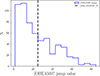 |
Fig. 1. Distribution of jumps for SagDIG H II region spectral fibres shown in blue. The vertical dashed black line indicates the lower limit (25) used to select those fibres in which the integrated spectra of SagDIG H II show the auroral line with S/N > 3. |
The integrated spectrum representing the SagDIG H II region is shown in the left and middle panels of Figure 2, where the auroral [O III]λ4363 line is marked with a red arrow. The spatial distribution of the spectral fibres with jump > 25 is shown in the right panel of Figure 2, where the colour code represents the jump value per spaxel. The Hβ emission line map (grey contours) of the complete data cube is superimposed for reference.
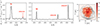 |
Fig. 2. Integrated spectrum of the SagDIG H II region. The left panel shows the window wavelength of the Hγ and [O III]λ4363 emission lines. The middle panel shows the Hβ and [O III]λλ4959,5007 emission lines. The right panel shows the spatial distribution of the selected fibres to generate the integrated spectrum of the SagDIG H II region with auroral detection. The colour code represents the jump value of each selected fibre. The grey contours represent the Hβ emission of the nebula as reference. |
In our reduced and integrated spectrum, we do not detect underlying stellar absorption in the recombination lines of H. Therefore, no additional subtraction was done after the data reduction. Single Gaussian functions were fitted to all available emission lines for the SagDIG integrated spectrum. To correct for internal absorption due to dust, we performed the Balmer decrement corrections. When available, the procedure consists in using the theoretical H recombination emission line ratio, IHα/IHβ = 2.85 (Hummer & Storey 1987), adopting Case B (Te≃104K). However, the Hα emission line falls outside the spectral coverage of the VIMOS-IFU observations used in this work. Therefore, following Hummer & Storey (1987), we used the theoretical IHβ/IHγ = 2.137 emission line ratio assuming Case B. The correction is as follows: The reddening constant was calculated as CHγ=[log(IHβ/IHγ)−log(FHβ/FHγ)]/[f(Hβ)−f(Hγ)], where f(λ) = 〈A(λ)/A(V)〉 is the extinction law at a given wavelength. Following Cardelli et al. (1989), we adopted RV = 3.1. Lastly, the emission line measurements were corrected applying Iλ/IHγ=(Fλ/FHγ)×10CHγ[f(λ)−f(Hγ)]. The emission line flux measurements are shown in Table 1.
Emission line flux measurements of the SagDIG H II region integrated spectrum.
2.3. EFOSC2 data
In order to estimate the total oxygen abundance and explore variations in the different ionisation states of oxygen across the SagDIG H II region, the [O II]λ3727 emission line measurement is also needed. For this reason, we used the archival long-slit data from the ESO Faint Object Spectrograph Camera (v.2; EFOSC2, Buzzoni et al. 1984), presented in Saviane et al. (2002). The observations were taken in August 2000 (PI: Y. Momany) under the programme 63.N-0726(B), at the ESO observatory in La Silla, Chile. The EFOSC2 is a versatile instrument for low-resolution spectroscopy and imaging, and it was attached to the ESO 3.6m telescope at the time of the observations. The EFOSC2 observations consist of 4×1200 s exposures using grism #7 (327–5250 nm, and 0.96 Å px−1 dispersion) and grism #9 (470–677 nm, and 1 Å px−1 dispersion), both with a 1.5″ slit.
Each scientific frame was reduced independently with the Image Reduction and Analysis Facility (IRAF1) software. We performed bias subtraction, flat normalisation, wavelength calibration, and flux calibration at each position along the slit, which covers the H II region. We selected 10 slit pixels outside the H II region to extract the sky spectrum and stellar continuum and applied the subtraction to each slit pixel of the H II region. The flux calibration was done by using a spectrophotometric standard star from Hamuy et al. (1992, 1994): namely, the G-type LTT-1020 (V = 11.52, B−V = 0.56). The final products were flux-calibrated in units of 10−16 erg s−1 cm−2 Å−1. The dust reddening correction was applied in the same way as the VIMOS-IFU data. The flux-calibrated 2D frame is shown in Figure 3, with the detected emission lines shown in yellow.
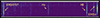 |
Fig. 3. EFOSC2 long-slit, flux-calibrated 2D frame of the SagDIG H II region. Yellow arrows show the detected emission lines in each slit column. |
3. Data analysis
3.1. Spatially resolved flux distributions
Once the VIMOS-IFU fibre spectra were reduced, we proceeded to study the gas-phase structures of the SagDIG nebula. The flux distributions presented in this subsection were constructed by measuring the flux of the detectable (S/N > 3) strong emission lines Hβ and [O III]λ5007, fitting Gaussian curves to each continuum and sky-subtracted spectrum for all spectral fibres of the VIMOS cube.
Figure 4 shows the SagDIG H II region spatial flux distribution for Hβ in the left panel and the [O III]λ5007 in the right panel. Dashed grey circles with increasing radius from 1.34″ (2 px) up to 12.06″ (18 px) are also shown for a subsequent analysis of the flux density profiles, centred at α = 19h30m3.2s, δ=−14°41′29.94″ (J2000). The centre was determined as the intermediate point between the two Hβ clumps. Additionally, we applied bilinear interpolation in the flux maps to smooth out spatial variations between the pixels and to remove artefacts.
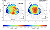 |
Fig. 4. SagDIG H II region emission line maps. The left panel shows the Hβ emission line distribution. The right panel shows the [O III]λ5007 emission line distribution. The colour map represents the flux at each emission line. The dashed grey lines indicate circles of increasing radius of 1.34″ (2 px) up to 12.06″ (18 px). The dotted black lines show the angles that separate the S clump, the NE tail, and the NW clump. |
The Hβ flux distribution reveals that the SagDIG H II region has two main clumps: one in the southern region and the other one in the north-west direction, both at ∼5″ from the centre. We also note a small tail-like structure from the centre in the left panel towards the north-east up to ∼8″.
The right panel of Figure 4 shows the [O III]λ5007 flux distribution. This seems to cover a larger area on the map than the Hβ emission, which is indicated with reddish colours out to ∼8″ from the centre. This is even clearer with the composite image created with the left and right panels of Figure 4, as shown in Figure 5, where blueish and reddish colours represent the Hβ and [O III]λ5007 emission, respectively.
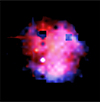 |
Fig. 5. Composite image of the flux distribution shown in Figure 4. The blue colour represents the Hβ flux distribution, and the red colour represents the [O III]λ5007 flux distribution. |
Radial flux density profiles were generated to study the Hβ and [O III]λ5007 structures. These are defined as Σλ=∑Fλ/Aring, where ∑Fλ is the sum of the flux of a given emission line from the fibres inside the area between two consecutive concentric circles of radii, rin and rout, described as
 (1)
(1)
as shown in Figure 4. ϕ0 and ϕf are the angles that contain each structure (clockwise along the x-axis from the centre of the concentric circles, from left to right), i.e. the southern clump, the north-west clump, and the north-east tail-like structure.
To generate the southern clump (hereafter, S clump) flux density profile, we selected all the fibres between 20°<ϕ<150°. The north-east tail-like structure (hereafter, NE tail) radial profile was produced by selecting fibres between 170°<ϕ<230°. Lastly, the north-west clump (hereafter, NW clump) radial profile was produced by using the fibres between 240°<ϕ<360°. The angular selection of the Hβ structures is shown by the dotted black lines in both panels of Figure 4. The flux density profiles have units of 10−16 ergs s−1 cm−2 Å−1 arcsec−2.
The top and middle panels of Figure 6 show the Hβ, and [O III]λ5007 radial flux density profiles, respectively, for the three structures. The black lines represent the S clump, the red lines represent the NW clump, and the blue lines represent the NE tail.
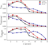 |
Fig. 6. Flux density profiles for the S clump, NW clump, and NE tail structures present in the SagDIG nebula, indicated by black dots, red squares, and blue triangles, respectively. The top panel shows the Hβ flux density profiles. The middle panel shows the [O III]λ5007 flux density profiles. The bottom panel shows the [O III]λ5007 / Hβ flux density profile. |
The upper panel of Figure 6 indicates that both the S clump and the NW clump are similar in terms of Hβ flux density. Both increase in flux density, reaching a peak between ∼4″−6″, then decrease in flux density up to ∼8″ and ∼9″ for the S clump and NW clump, respectively.
Both clumps show similar behaviour in terms of the [O III]λ5007 flux density. However, the [O III]λ5007 flux density is almost twice the Hβ flux density. Both peak at ∼3″. Comparing the Hβ and the [O III]λ5007 flux densities, the latter is more concentrated in the centre than the former. On the other hand, the NE tail shows a different flux density distribution in Hβ and a lower flux-density with respect to the clumps. However, although the [O III]λ5007 flux density profile of the NE tail shows a gradual radial decrement, the profile is similar to those of the clumps, suggesting that the distribution of oxygen is more symmetric in the H II region compared to the hydrogen flux distribution.
The bottom panel of Figure 6 presents the flux density profile of the emission line ratio [O III]λ5007/Hβ for the three substructures. The flux-density profiles of both clumps reveal similar trends: the S clump shows values closer to 1, while the NW clump exhibits values slightly greater than 1. In addition, both flux-density profiles show a decrease in their emission line ratio for radii greater than 6″. This feature suggests that O++ is more centrally concentrated with respect to H+. Otherwise, the flux density profile of this emission line ratio would show a flat behaviour.
The Hβ and the [O III]λ5007 emission maps and flux density profiles show signs of ‘stratification’ in the H II regions (Osterbrock & Ferland 2006): the SNe explosions and UV radiation from massive stars (OB spectral type) located in the H II regions can inject a huge energy budget into their surrounding gas. Because radiation density decreases with distance, the central regions host a highly ionised species (such as O++), whereas the outskirts host a lower ionisation species (such as H+, O+, N+, and S+), where the H+ prevails over O++. This creates a stratified ionisation structure with different ionised zones for different atoms, as seen in certain galactic H II regions as well as in the Large Magellanic Cloud (Sánchez 2013; Barman et al. 2022; Kreckel et al. 2024).
3.2. The search for stratification in the EFOSC long-slit data
In this section, we employ the EFOSC2 long-slit spectrum to further study the ionisation stratification of the H II region using a more direct approach that compares two oxygen ionisation levels (O+ and O++). The slit position in the SagDIG H II region is shown in the left image of Figure 7, which corresponds to the pre-imaging frame of the EFOSC2 long-slit observations.
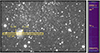 |
Fig. 7. Left panel: EFOSC2 pre-imaging frame of the SagDIG H II region. The yellow rectangle shows the slit position used to extract the 2D frame spectra. The vertical yellow lines indicate the area covered by the H II region, from column 280 to column 320. Right panel: 2D frame spectra, where the emission lines detected are indicated by yellow arrows. |
The slit position is shown with the yellow rectangle, and the vertical yellow lines indicate the position along the slit where the SagDIG H II region is covered (x = 280 to x = 320). The right image of Figure 7 shows the spectra of the SagDIG H II region inside the slit area from pixel 280 to 320 in the 2D frame from left to right, respectively. As seen in the right panel of Figure 7, the Hβ, Hγ, [O II]λ3727, and [O III]λλ4959,5007 emission lines are detected.
To confirm the stratification, it is necessary to determine whether O+ is spatially distributed (across the slit region covered) in a similar way to H+, with respect to O++. Therefore, we proceed to study the emission line ratios [O III]λ5007/Hβ and [O III]λ5007/[O II]λ3727 as a function of the position along the slit. It is important to note that the position along the slit represents the spatial coordinates on the x-axis. Therefore, we study here the behaviour of the emission line ratios in the east-west direction within the slit area that covers the H II region.
Figure 8 presents the distribution of the emission line ratios between Hβ, [O II]λ3727, and [O III]λ5007 along the slit. The x-axis represents the position along the slit, where 0 is the centre of the H II region used in Figure 4. The upper panel of Figure 8 presents the emission line ratios [O III]λ5007/Hβ and the [O III]λ5007/[O II]λ3727, with green dots and purple squares, respectively, together with a second degree polynomial fitting for each emission line using the same colours. This panel reveals that both emission line ratios behave similarly, showing higher values of emission line ratios at the centre compared to the outskirts. The lower panel presents the emission line ratio [O II]λ3727/Hβ with black dots, along with its respective linear fit shown as a grey line. This reveals that the emission line is flat across the position along the slit, at [O II]λ3727/Hβ ∼1.6. The linear fit suggests a slope 0.004±0.006.
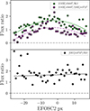 |
Fig. 8. Emission line ratios across the slit column, representing east-west coordinates in the SagDIG H II region. The upper panel shows the [O III]λ5007/Hβ and the [O III]λ5007/[O II]λ3727 emission line ratios, with green dots and purple squares, respectively. The lower panel shows the [O II]λ3727/Hβ emission line ratio with black dots. |
These panels indicate that (i) O++ is more concentrated at the centre of the H II region compared to both O+ and H+, and (ii) O+ is distributed in a way similar to H+ along the slit area that covers the H II region. These features yield the same information as the emission line maps and the flux-density profiles shown in Figure 6 and Figure 7. This hence confirms that the SagDIG H II region is a dynamic nebula.
3.3. Te-based oxygen abundances
Our aim was to estimate oxygen abundances with the so-called ‘direct method’ (Peimbert 1967; Aller 1984; Izotov et al. 2006). We thus used the integrated spectrum of the SagDIG H II region in order to estimate metallicities. This method uses emission line ratios sensitive to the electron temperature, Te, together with the computation of the corresponding line emissivities. The estimated values are available in Table 2 and are discussed in Appendix A.
Electron temperature and ionic oxygen abundances estimated for SagDIG.
The Te-sensitive emission line ratios are estimated by using weak auroral lines such as [O III]λ4363 and [N II]λ5755. Measuring the auroral line in each spectrum fibre is quite difficult because this emission line is ∼3−4 orders of magnitudes fainter than the Balmer emission lines (Maiolino & Mannucci 2019), and can be lost in the spectral noise. Using the integrated spectra reduces the spectral noise compared to the individual fibre spectra. As seen in Figure 2, the integrated spectrum of SagDIG shows the auroral [O III]λ4363 emission line with S/N>3.
This method also requires the electron density, Ne, to compute the oxygen abundances. However, our data does not cover the wavelength range for the estimation of Ne through emission lines such as [S II]λλ6717,6731. We hence assumed Ne = 100 cm−3 according to the low-density limit (Hummer & Storey 1987).
We used the [O III](λ4959+λ5007)/λ4363 emission line ratio to estimate Te([O III]). We did this by using the getTemDen module of the Pyneb python package (Luridiana et al. 2015). We then calculated Te([O II]) by using the linear relation, Te([O II]) = 0.7×Te([O III])+3000, calibrated by Campbell et al. (1986) from the Stasińska (1982) photoionisation models.
The Te-based oxygen abundance was estimated using two different approaches: (i) the getIonAbundance Pyneb module, which uses Eq. 4 of Luridiana et al. (2015); and (ii) Eq. 3 and Eq. 5 from Izotov et al. (2006, hereafter, I06), which were estimated by using photoionisation grid models of H II regions. Both equations of I06 require that Te be used in order to estimate the ionic oxygen abundances O+/H and O++/H. We thus used the estimated values from the getTemDen Pyneb module for Te. The Te estimates are shown in Table 2.
We derived Te = 17 683±1254 accouting for the integrated spectrum of the SagDIG H II region (Table 1 and Figure 2). The total oxygen abundance is defined as 12+log(O/H), where O/H=(O+/H++O++/H+). The VIMOS-IFU spectral range does not cover the wavelength region where [O II]λ3727 is found. For this reason, we used the [O II]λ3727 flux measurement from S02 to estimate the O+/H ionic abundance. However, that measurement comes from a 1.5″ EFOSC2 long-slit spectrum, covering the central part of the H II region, as shown in Figure 7. The combination of the VIMOS-IFU integrated spectrum and the EFOSC2 long-slit spectrum can introduce both instrumental biases and aperture effects. For this reason, we reproduced a mock-slit in the VIMOS IFU data following the EFOSC2 long-slit observations of S02. Our mock-slit is 2px wide, i.e.  , and has the same position and orientation as S02.
While the mock-slit aperture is slightly narrower than the actual slit employed in S02, and despite likely imperfect centring, we find that the EFOSC2 and mock-slit measurements yield ionic O++/H abundances in excellent agreement. Therefore, we derived a tentative Te-based metallicity by combining the EFOSC2 measurements of the [O II]λ3727 emission line with the Te obtained from the VIMOS mock-slit [O III]λ4363 emission line, together with the lines common to both datasets. The complete procedure for the different approaches to estimate Te and oxygen abundances is described in Appendix A.
We derived Te[O III] = 22 165±1122 K, Te[O II] = 18 515±987 K, and a Te-based total oxygen abundance of 12+log(O/H) = 7.23±0.04 dex using Pyneb. However, the I06 calibration results in 12+log(O/H) = 7.00±0.03 dex. The discrepancy between Pyneb and I06 Te-based oxygen abundances has been previously explored by Laseter et al. (2024) in a sample of high-redshift galaxies, showing differences (∼0.1 dex on average and 0.2 dex in extreme cases) consistent with our results. Further investigation led us to conclude that the difference in metallicities is produced by the estimated O+/H, as shown in Table 2, probably because I06 provides an empirical relation between the flux [O II]λ3727 and Te[O III] with the ionic abundance O+/H. Therefore, we use the Pyneb Te-based oxygen abundances to interpret the results presented in Section 4. The difference between the Te-integrated spectrum and the mock-slit suggests temperature fluctuations in the SagDIG H II region with subsequent aperture effects.
3.4. Intrinsic biases of the Te−sensitive method
Several studies in the literature have discussed the well-known biases affecting the direct method (Kobulnicky & Skillman 1996; Pilyugin & Grebel 2016; Cameron et al. 2023). These biases include: (i) temperature fluctuations, which in general lead to overestimated temperatures and subsequent underestimated metallicities, because of the dependence of the emissivities on the statistical factor e−hν/kTe (Aller 1984; Osterbrock & Ferland 2006; Maiolino & Mannucci 2019); (ii) different ways of estimating the electron temperature, such as the use of emission line ratios as well as Balmer or Paschen jumps (Peimbert 1967); and (iii) O++ abundances estimated from recombination lines, which can yield metallicities up to three times higher than those estimated from the collisional excitation lines (Esteban et al. 2014). Despite these biases, the direct method is still the best choice for estimating oxygen abundances, because the so-called ‘empirical methods’ (which make use of different strong emission lines depending on the choice of the calibrator) show oxygen abundance differences of up to 0.7 dex among them (Kewley & Ellison 2008; Poetrodjojo et al. 2021).
We are able to address the temperature fluctuation problem, since our integrated spectrum has a detectable [O III]λ4363 emission line. Specifically, Cameron et al. (2023) used the Katz (2022) dwarf galaxy (Mhalo = 1010 M⊙, Mgas = 3.5×10⁸ M⊙, and central metallicity of 0.1 Z⊙) simulated with the RAMSES-RTZ code. They tackled the temperature fluctuation problem by introducing the ‘line temperature’, Tline, which links the emissivities of the emission lines along a range of probed temperatures (see their Figure 1). With this approach, the authors report the relation Tline = 0.6Tratio+3258 K, where Tratio is the standard Te estimated from the [OIII] ratio.
Applying the Tline correction, we obtain 12+log(O/H)corr = 7.50±0.08 (Tline = 16 557±1093) with our flux measurements. The correction leads to an increase in the oxygen abundances of ∼0.3 dex.
3.5. Te and oxygen abundance spatial variations in the SagDIG H II region
In Section 3.3 we show that the Te of the H II region is ∼22100 K. However, it is possible to explore Te and metallicity variations inside the area covered by the EFOSC2 observations (coloured area in Figure 9). This is because we flux-calibrated the 2D frame of the S02 long-slit data (Section 2.3). To explore possible spatial variations, we (i) selected a central and external region in the VIMOS-IFU simulated slit to estimate Te and the ionic abundance O++/H and (ii) applied the same spatial cuts in the EFOSC2 2D frame (Figure 9) in order to measure the corresponding [O II]λ3727 emission line flux and a subsequent O+/H ionic abundance, for a central and external region of the H II region.
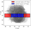 |
Fig. 9. Simulated slit in the IFU data following the EFOSC2 long-slit observations of S02 compared to the [O III]λ5007 emission line map indicated by the black contours. The simulated slit was divided into four sections of equal area, where the first and fourth represent the external region in red, and the second and third represent the central region in blue, from left to right, respectively. |
We divided the simulated slit into four sections of the same area, where the external region is defined as the first and fourth sections, and the central region is defined as the second and third section from left to right, as shown in Figure 9 in red and blue. The same was done in the 2D frame for the EFOSC-long slit data. Each section in the simulated slit in the VIMOS-IFU data is 7px long. Both the central and external regions hence cover 14px long, which is 9.4″. The central region has a Te = 23 390±1096 and 12+log(O/H) = 7.24±0.05, whereas the external region has a Te = 21 941±2572 and 12+log(O/H) = 7.50±0.08, showing a decrease of ∼1500 K and an increase of ∼0.25 dex towards the outskirts.
On the other hand, the individual ionic abundances for the central region and external are 12+log(O+/H) = 7.06±0.06 and 12+log(O++/H) = 6.78±0.04, and 12+log(O+/H) = 7.45±0.15 and 12+log(O++/H) = 6.53±0.12, respectively. These results suggest that (i) the centre is slightly hotter and more metal-poor than the outskirts, (ii) the centre has more O++ ionic abundance than the outskirts, and (iii) the outskirts have more O+ ionic abundance than the centre, in line with the stratified composition of the SagDIG H II region observed in Sections 3.1 and 3.2.
4. Results and discussion
4.1. The role of star formation in the SagDIG H II region
Using HST photometry to explore SagDIG's stellar populations, Momany et al. (2005) reported a young main sequence (MS), indicative of an ongoing star-formation episode, as well as a well-defined red giant branch, suggesting that SagDIG also experienced an extended star-formation episode between 1 and 9 Gyr ago. The suggestions from these features were confirmed by SFHs derived by Held et al. (2007), and Parto et al. (2023). The old stars are uniformly distributed across the SagDIG structure. On the other hand, young MS stars are located closer to the high H I gas density clump previously studied by Young & Lo (1997).
To analyse the spatial distribution of stars located inside the H II region, we applied cuts on the SagDIG's colour-magnitude diagram (CMD) similar to those of Momany et al. (2005), as shown in the right panel of Figure 10. Old RGB stars and red clump stars (∼1−9 Gyr) as 0.5<F475W−F606W<1.2 (white dots), and young MS stars (31−630 Myr) are selected as F475W−F606W<0.3 and F606W<26.5 (cyan dots and crosses), where the most luminous MS star is marked with an orange star, and the second and the third ones are indicated with magenta and green crosses, respectively.
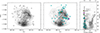 |
Fig. 10. Comparison of the SagDIG H II region Hβ emission (black contours) with the stellar HST photometry from Momany et al. (2005). The left panel shows the old RGB and red clump stars (white dots) in the H II region. The middle panel shows the distribution of young MS stars (<7 M⊙ and 7−10 M⊙, indicated by cyan dots and cyan crosses, respectively) in the H II region. The orange star is the most luminous (15 M⊙), and the magenta and green crosses are the second and third (>10 M⊙) most luminous stars. The right panel shows the CMD of SagDIG, with the same symbols and colours as in the left and the middle panel. The vertical black curve is a 10 Myr isochrone, showing the MS of young stars to provide a proxy for the stellar masses of the young stars. The horizontal black lines show the corresponding range of masses in the main sequence. |
The spatial distribution of the selected old RGB and red clump stars in the H II region (black contours) is shown in the left panel of Figure 10. These stars are uniformly distributed. However, the young MS stars do not follow the same trend, as seen in the middle panel. These MS stars are located closer to the edges of the southern and the north-west Hβ clumps in a filamentary-like configuration, and the most luminous star is located near the centre of the biconic-like distribution.
Stars are born in high gas-density regions, where the ionising flux of young massive stars expels the surrounding gas. This results in either denser gas regions with stars located in situ, and/or crowded regions of stars surrounded by an ionised gas structure. Therefore, the spatial distribution shown in the middle panel of Figure 10 is not expected.
The spatial distribution of young MS stars could be produced by an observational bias: the clumps of the Hβ emission may indicate potential regions of active star formation, so it is possible that those zones could contain significant dust that prevents us from detecting young stars, i.e. high C(Hγ) values (or high Hβ/Hγ ratio) compared to the remaining zones of the H II region. However, the reddening constant, C(Hγ), shows a flat behaviour across the H II region. Therefore, the spatial distribution of the SagDIG stars in the H II region must be due to a physical phenomenon.
As shown in the right panel of Figure 10, a 10 Myr PARSEC isochrone (Bressan et al. 2012) was used, adopting Z = 0.004 and AV = 0.62 (Momany et al. 2005) to provide a proxy for stellar masses of the young MS stars, suggesting that the most luminous star has a mass of 15 M⊙ (orange star), and the second and third most luminous stars have masses in the range 10−15 M⊙. The middle panel of Figure 10 shows that the 15 M⊙ is located near the centre, whereas the two stars between 10 and 15 M⊙ are located at the edges of the biconic-like shape.
In order to better understand the SagDIG H II region, we visually inspected the HST image acquired from Momany et al. (2005), shown in Figure 11. The left panel shows the distribution of the old stellar population marked with yellow squares, whereas the right panel shows the distribution of the young stellar population marked with cyan circles. As seen, the horizontal filamentary structure is clearly visible in the right panel, and the diagonal filamentary structure seems to be a mix of clumps of stars aligned. In addition, there is a large vertical emitting structure likely formed by unresolved young stars, which are not in the Momany et al. (2005) photometric catalogue.
 |
Fig. 11. HST image (F475W, F606W and F814W combined) acquired by Momany et al. (2005) observations, showing the SagDIG H II region. The left panel shows the location of the old stellar population marked with yellow squares. The right panel shows the young stellar population marked with cyan circles. In both panels, the vertical diffuse column density is indicated with the red arrow. The source in the upper right region is a foreground star. |
OB-type MS stars are able to ionise their surrounding gas by radiation pressure in UV wavelengths, where the range of the observed wind velocities in OB stars goes up to a few hundred km s−1 (Lamers & Cassinelli 1999, Lamers & Levesque 2017, Osterbrock & Ferland 2006). However, there are stars with masses <10 M⊙, covering ages up to 630 Myr (Momany et al. 2005) located at the edges of the lobes, suggesting that the two-lobe structure was created before the ionising stars in the centre were born. This feature is also in line with observational studies, which suggest that stellar outflows can trigger sequential star formation, setting age gradients across H II regions (Matsuyanagi et al. 2006, Ogura et al. 2007, Rygl et al. 2014). Hence, a mix between SNe explosions and UV ionisation from massive stars likely shapes the evolution of the H II region.
Because the SagDIG H II region is expanding and is located at the edge of the densest H I density clump (Young & Lo 1997), the interaction between the H I component and the gas ionised from massive stars and SNe explosions could somehow create the filamentary structures of young stars. The H II regions show complex morphologies depending on ionising sources, non-uniform gas distributions, and young stellar objects frequently detected in such layers and filamentary gas structures as those found in the Orion nebula, the Eagle nebula, the Rosette nebula and other galactic H II regions (Hill et al. 2012, Tremblin et al. 2014, Zavagno et al. 2020, Gaudel et al. 2023). The existence of filamentary structures has been known since the last century (Schneider & Elmegreen 1979, Ungerechts & Thaddeus 1987), but only Herschel observations were able to link the existence of those objects with star formation (André et al. 2010, Molinari et al. 2010). However, although their properties are well identified, they are poorly constrained. High-resolution observations will help us get an understanding of their formation and evolution, putting new constraints on the underlying physics employed by theoretical simulations (e.g. Xu et al. 2019).
The interaction between the H I material and H II regions for the formation of filaments is still an open question (see discussion in Zavagno et al. 2020), but important clues were given by Tremblin et al. (2014), which demonstrate that the ionisation feedback (compression of the material induced by the expansion of ionised gas) is key in assembling material in the photo-dissociation region (PDR) to form filamentary structures. Theoretically, the turbulent gas compressed by UV radiation from OB stars may trigger star formation (Menon et al. 2020). However, few observational studies suggest that the net effect of the ionised radiation and stellar winds can trigger star formation (Billot et al. 2010, Chauhan et al. 2011, Roccatagliata et al. 2013).
4.2. The sagDIG H II region in the mass-metallicity plane
Analysing the physical structure of the H II region with both the VIMOS-IFU and the EFOSC2-long slit data provided us with important insights into the physical mechanisms shaping the evolution of the gaseous nebula. These insights can also be constrained by the gas-phase chemical content. Therefore, we place the SagDIG H II region in the mass-metallicity plane. It is important to note that we use the total stellar mass of SagDIG and assume that the metallicity of the only known H II region is representative of the whole galaxy. Therefore, the inferred properties should be interpreted with caution, considering the potential uncertainties and the limited sample size.
We used 1.8±0.5×10⁶ M⊙ as the stellar mass of SagDIG from Kirby et al. (2017). This value is based on the stellar mass-to-light ratios of Woo et al. (2008). Because of the biases discussed in Section 3.4, we considered both the Te corrected and the uncorrected gas-phase metallicities of the SagDIG H II region (from the VIMOS-IFU data), since most of the studies that employ this method do not take into account this bias. Figure 12 shows SagDIG in the mass-metallicity plane marked with a white triangle and white dot as the corrected and uncorrected oxygen abundances by Te fluctuations, respectively. We compare these values with the Te-based local Universe MZR of Andrews & Martini (2013) and Curti et al. (2020). In addition, we also compare our results with the low-mass end of the MZR of Lee et al. (2006) and Berg et al. (2012). Colour contours represent the galaxy sample of dIrr galaxies used to fit the low-mass end of the MZR in both studies.
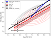 |
Fig. 12. SagDIG in the mass-metallicity plane marked with a white triangle and white dots for the Te corrected and uncorrected oxygen abundance, respectively. The dotted black and solid blue lines are the local Universe Te−based MZR of Curti et al. (2020) and Andrews & Martini (2013). The black and solid red lines represent the low-mass end of the MZR from Lee et al. (2006) and Berg et al. (2012). The contours represent the respective galaxy sample of dIrr galaxies used to fit the low-mass end of the MZR marked with corresponding colours. The dashed red area indicates the respective scatter of σ = 0.15 dex of the Berg et al. (2012) low-mass end of the MZR. |
The intrinsic scatter of the MZR increases as the metallicity and mass decrease (Zahid et al. 2012), because low-mass galaxies are more likely to be disturbed by pristine gas inflow and outflow mechanisms, in which the gas flows in these systems can change how efficiently the gas can form stars (Peeples et al. 2008, Davé et al. 2011, Lilly et al. 2013). Therefore, the non-equilibrium regime put a galaxy outside the main locus of the low-mass end of the MZR. In particular, outflow processes from SNe explosions in low-mass galaxies have a significant impact because they act on shallower potential wells. Hence, it is inherent to conclude that, in general, the evolution of a low-mass metal-poor galaxy is truncated when outflow mechanisms act, expelling metals with a high mass-loading factor (Chisholm et al. 2018).
Zoom-in hydrodynamical simulations demonstrate that small galaxies (Mdyn<108 M⊙) grow in stellar mass up to z∼4 as a consequence of cosmic reionisation, where the strong stellar feedback driven by galactic winds increases the ISM temperature, preventing the gas infall onto those galaxies (Agertz et al. 2020; Rey et al. 2024). This results in a slow chemical evolution in dwarf galaxies, which is in line with the observational evidence of suppression of star formation at early epochs in dwarf galaxies (Held et al. 2007, Cole et al. 2007, Tolstoy et al. 2009). Hence, the shallower slope at the low-mass end of the MZR can begin to be observed from the high-redshift Universe (z>6, Curti et al. 2023) to the local Universe (Lee et al. 2006, Berg et al. 2012), likely shaped by galaxies affected by outflows triggered by momentum-driven SNe winds, according to the theoretical models from Murray et al. (2005), and Davé et al. (2012). As viewed in Figure 12, the location of SagDIG in the mass-metallicity plane falls inside the 1σ scatter (0.15 dex) at the low-mass end of the MZR, suggesting that the SagDIG H II region is likely dominated by low-scale outflows processes, in line with the features observed in the previous subsections.
The observed stratification of the ionised gas, revealed by the emission line maps and flux-density profiles, and the filamentary configuration of the young stellar populations, together with their low-metallicity content (which places SagDIG in the low-mass end of the MZR), all suggest that the scenario best explaining the observed features of the SagDIG H II region, is one in which the gaseous structure is dominated by stellar feedback processes, such as ionisation from massive stars, SNe explosions, and stellar winds. This would mean that extragalactic H II regions in the local Universe are governed by similar underlying physics as the H II regions in the Milky Way.
This proposed scenario should be tested with (i) a kinematic analysis of the ionised gas, (ii) an exploration of other atomic species (such as N+, and S+), (iii) infrared observations to study the dust content and the filamentary structures, and (iv) UV observations to get information on stellar winds from massive OB stars. High performance instruments, (e.g. MUSE/VLT, NIRSpec/JWST, and MIRI/JWST) will help to disentangle the nature of the evolution of the SagDIG H II region with better spatial resolution and spectral coverage.
5. Summary and conclusions
This work presents, for the first time, a detailed analysis of an H II region beyond the Milky Way. We used archival optical, intermediate-resolution VIMOS/VLT-IFU and EFOSC2/NTT-long slit data to explore the physical structure of the only known H II region in SagDIG, to probe the physical mechanisms shaping the chemical evolution of this nebula. We detected the auroral [O III]λ4363 emission line and estimated oxygen abundances with the direct method, integrating the spectral fibres covering the H II region. The IFU data allowed us to generate emission line maps and flux-density profiles of Hβ and [O III]λ5007 in order to study their structures. Furthermore, the EFOSC2 long-slit data allowed us to explore emission line flux variations in the east-west direction of the H II region with more emission lines than the IFU data.
The analysis done in this work suggests that the H II region of the metal-poor dwarf galaxy SagDIG shows a similar evolution to galactic H II regions. Our main conclusions are summarised as follows:
-
The SagDIG H II region shows two prominent Hβ clumps. The flux-density maps reveal that those clumps are similar in terms of size and flux, in the Hβ and [O III]λ5007 emission lines. They also seem to be aligned across the same axis.
-
The O++ distribution is more concentrated towards the centre compared to such low ionisation species as O+ and H+, suggesting that the stratified composition of this nebula is due to ongoing expansion.
-
The young stellar population, located closer to the edges of the two clumps, is distributed in a filamentary-like configuration, whereas the old stellar population is uniformly distributed across the H II region. These features suggest that stellar feedback mechanisms, such as UV radiation from massive stars, stellar winds, and SNe explosions, are likely the main physical phenomena shaping the evolution of this nebula.
-
The direct method Te−based oxygen abundance of the SagDIG H II region is 12+log(O/H) = 7.23±0.04, or 12+log(O/H) = 7.50±0.08 with the Cameron et al. (2023) temperature correction applied.
-
The SagDIG H II region shows spatial variations in terms of decreasing Te and increasing Te−based oxygen abundances of ∼1500 K and ∼0.25 dex towards the outskirts, respectively, in line with the stratified composition.
-
The position of SagDIG in the mass-metallicity plane is consistent with the low-mass end of the MZR, suggesting that the H II region is dominated by stellar feedback mechanisms.
Acknowledgments
We thank the anonymous referee for their useful comments which improved the quality of the paper. A special thanks goes to Eric Andersson, Joseph Anderson, Bastian Ayala, Ana Jimenez, Timo Kravtsov, Thomas Moore, and Felipe Vivanco Cádiz for the opportunity to discuss our results. L.M. acknowledges support from ANID-FONDECYT Regular Project 1251809.
IRAF is distributed by the National Optical Astronomy Observatories, which are operated by the Association of Universities for Research in Astronomy, Inc., under a cooperative agreement with the National Science Foundation.
References
- Agertz, O., Pontzen, A., Read, J. I., et al. 2020, MNRAS, 491, 1656 [Google Scholar]
- Aller, L. H. 1984, Astrophysics and Space Science Library (Dordrecht: Reidel) [Google Scholar]
- André, P., Men'shchikov, A., Bontemps, S., et al. 2010, A&A, 518, L102 [CrossRef] [EDP Sciences] [Google Scholar]
- Andrews, B. H., & Martini, P. 2013, ApJ, 765, 140 [NASA ADS] [CrossRef] [Google Scholar]
- Astropy-Specutils Development Team 2019, Astrophysics Source Code Library, [record ascl:1902.012] [Google Scholar]
- Atek, H., Labbé, I., Furtak, L. J., et al. 2024, Nature, 626, 975 [NASA ADS] [CrossRef] [Google Scholar]
- Barman, S., Neelamkodan, N., Madden, S. C., et al. 2022, ApJ, 930, 100 [NASA ADS] [CrossRef] [Google Scholar]
- Benítez-Llambay, A., Navarro, J. F., Abadi, M. G., et al. 2015, MNRAS, 450, 4207 [CrossRef] [Google Scholar]
- Berg, D. A., Skillman, E. D., Marble, A. R., et al. 2012, ApJ, 754, 98 [NASA ADS] [CrossRef] [Google Scholar]
- Billot, N., Noriega-Crespo, A., Carey, S., et al. 2010, ApJ, 712, 797 [NASA ADS] [CrossRef] [Google Scholar]
- Bressan, A., Marigo, P., Girardi, L., et al. 2012, MNRAS, 427, 127 [NASA ADS] [CrossRef] [Google Scholar]
- Bunker, A. J., Wilkins, S., Ellis, R. S., et al. 2010, MNRAS, 409, 855 [Google Scholar]
- Burkhart, B., Stanimirović, S., Lazarian, A., et al. 2010, ApJ, 708, 1204 [NASA ADS] [CrossRef] [Google Scholar]
- Buzzoni, B., Delabre, B., Dekker, H., et al. 1984, The Messenger, 38, 9 [NASA ADS] [Google Scholar]
- Cameron, A. J., Katz, H., & Rey, M. P. 2023, MNRAS, 522, L89 [NASA ADS] [CrossRef] [Google Scholar]
- Campbell, A., Terlevich, R., & Melnick, J. 1986, MNRAS, 223, 811 [NASA ADS] [CrossRef] [Google Scholar]
- Cardelli, J. A., Clayton, G. C., & Mathis, J. S. 1989, ApJ, 345, 245 [Google Scholar]
- Cesarsky, D. A., Laustsen, S., Lequeux, J., et al. 1977, A&A, 61, L31 [Google Scholar]
- Chauhan, N., Pandey, A. K., Ogura, K., et al. 2011, MNRAS, 415, 1202 [NASA ADS] [CrossRef] [Google Scholar]
- Chisholm, J., Tremonti, C., & Leitherer, C. 2018, MNRAS, 481, 1690 [NASA ADS] [CrossRef] [Google Scholar]
- Cole, A. A., Skillman, E. D., Tolstoy, E., et al. 2007, ApJ, 659, L17 [Google Scholar]
- Cook, K. H. 1987, Ph.D. Thesis, Univ. Arizona, USA [Google Scholar]
- Curti, M., Mannucci, F., Cresci, G., et al. 2020, MNRAS, 491, 944 [NASA ADS] [CrossRef] [Google Scholar]
- Curti, M., D’Eugenio, F., Carniani, S., et al. 2023, MNRAS, 518, 425 [Google Scholar]
- Davé, R., Finlator, K., & Oppenheimer, B. D. 2011, MNRAS, 416, 1354 [CrossRef] [Google Scholar]
- Davé, R., Finlator, K., & Oppenheimer, B. D. 2012, MNRAS, 421, 98 [Google Scholar]
- Demers, S., & Battinelli, P. 2002, AJ, 123, 238 [Google Scholar]
- Dutta, P., Begum, A., Bharadwaj, S., et al. 2009, MNRAS, 398, 887 [Google Scholar]
- El-Badry, K., Quataert, E., Wetzel, A., et al. 2018, MNRAS, 473, 1930 [NASA ADS] [CrossRef] [Google Scholar]
- Emsellem, E., Schinnerer, E., Santoro, F., et al. 2022, A&A, 659, A191 [NASA ADS] [CrossRef] [EDP Sciences] [Google Scholar]
- Esteban, C., García-Rojas, J., Carigi, L., et al. 2014, MNRAS, 443, 624 [NASA ADS] [CrossRef] [Google Scholar]
- Finlator, K., & Davé, R. 2008, MNRAS, 385, 2181 [NASA ADS] [CrossRef] [Google Scholar]
- Freudling, W., Romaniello, M., Bramich, D. M., et al. 2013, A&A, 559, A96 [NASA ADS] [CrossRef] [EDP Sciences] [Google Scholar]
- Gaudel, M., Orkisz, J. H., Gerin, M., et al. 2023, A&A, 670, A59 [NASA ADS] [CrossRef] [EDP Sciences] [Google Scholar]
- Gullieuszik, M., Rejkuba, M., Cioni, M. R., et al. 2007, A&A, 475, 467 [NASA ADS] [CrossRef] [EDP Sciences] [Google Scholar]
- Hamuy, M., Walker, A. R., Suntzeff, N. B., et al. 1992, PASP, 104, 533 [NASA ADS] [CrossRef] [Google Scholar]
- Hamuy, M., Suntzeff, N. B., Heathcote, S. R., et al. 1994, PASP, 106, 566 [NASA ADS] [CrossRef] [Google Scholar]
- Held, E. V., Momany, Y., Rizzi, L., et al. 2007, Stellar Populations as Building Blocks of Galaxies, 241, 339 [Google Scholar]
- Hill, T., Motte, F., Didelon, P., et al. 2012, A&A, 542, A114 [NASA ADS] [CrossRef] [EDP Sciences] [Google Scholar]
- Hopkins, A. M., Miller, C. J., Nichol, R. C., et al. 2003, ApJ, 599, 971 [Google Scholar]
- Hummer, D. G., & Storey, P. J. 1987, MNRAS, 224, 801 [NASA ADS] [CrossRef] [Google Scholar]
- Hunter, D. A., Elmegreen, B. G., & Berger, C. L. 2019, AJ, 157, 241 [NASA ADS] [CrossRef] [Google Scholar]
- Hunter, D. A., Elmegreen, B. G., & Madden, S. C. 2024, ARA&A, 62, 113 [NASA ADS] [CrossRef] [Google Scholar]
- Izotov, Y. I., & Thuan, T. X. 2004, ApJ, 602, 200 [CrossRef] [Google Scholar]
- Izotov, Y. I., Stasińska, G., Meynet, G., et al. 2006, A&A, 448, 955 [CrossRef] [EDP Sciences] [Google Scholar]
- James, B. L., Tsamis, Y. G., & Barlow, M. J. 2010, MNRAS, 401, 759 [NASA ADS] [CrossRef] [Google Scholar]
- James, B. L., Tsamis, Y. G., Barlow, M. J., et al. 2013, MNRAS, 428, 86 [NASA ADS] [CrossRef] [Google Scholar]
- James, B. L., Kumari, N., Emerick, A., et al. 2020, MNRAS, 495, 2564 [NASA ADS] [CrossRef] [Google Scholar]
- Katz, H. 2022, MNRAS, 512, 348 [NASA ADS] [CrossRef] [Google Scholar]
- Kewley, L. J., & Ellison, S. L. 2008, ApJ, 681, 1183 [Google Scholar]
- Kirby, E. N., Rizzi, L., Held, E. V., et al. 2017, ApJ, 834, 9 [Google Scholar]
- Kobulnicky, H. A., & Kewley, L. J. 2004, ApJ, 617, 240 [CrossRef] [Google Scholar]
- Kobulnicky, H. A., & Skillman, E. D. 1996, ApJ, 471, 211 [NASA ADS] [CrossRef] [Google Scholar]
- Kreckel, K., Egorov, O. V., Egorova, E., et al. 2024, A&A, 689, A352 [NASA ADS] [CrossRef] [EDP Sciences] [Google Scholar]
- Kumari, N., James, B. L., & Irwin, M. J. 2017, MNRAS, 470, 4618 [NASA ADS] [CrossRef] [Google Scholar]
- Kumari, N., James, B. L., Irwin, M. J., et al. 2018, MNRAS, 476, 3793 [NASA ADS] [CrossRef] [Google Scholar]
- Lamers, H. J. G. L. M., & Cassinelli, J. P. 1999, in Introduction to Stellar Winds (Cambridge, UK: Cambridge University Press), 452 [Google Scholar]
- Lamers, H. J. G. L. M., & Levesque, E. M. 2017, in Understanding Stellar Evolution (Bristol, UK: IOP Publishing) [Google Scholar]
- Laseter, I. H., Maseda, M. V., Curti, M., et al. 2024, A&A, 681, A70 [NASA ADS] [CrossRef] [EDP Sciences] [Google Scholar]
- Le Fèvre, O., Saisse, M., Mancini, D., et al. 2003, Proc. SPIE, 4841, 1670 [NASA ADS] [CrossRef] [Google Scholar]
- Ledinauskas, E., & Zubovas, K. 2018, A&A, 615, A64 [NASA ADS] [CrossRef] [EDP Sciences] [Google Scholar]
- Lee, H., Skillman, E. D., Cannon, J. M., et al. 2006, ApJ, 647, 970 [NASA ADS] [CrossRef] [Google Scholar]
- Lilly, S. J., Carollo, C. M., Pipino, A., et al. 2013, ApJ, 772, 119 [NASA ADS] [CrossRef] [Google Scholar]
- Lin, Y. -H., Scarlata, C., Mehta, V., et al. 2023, ApJ, 951, 138 [Google Scholar]
- Luridiana, V., Morisset, C., & Shaw, R. A. 2015, A&A, 573, A42 [NASA ADS] [CrossRef] [EDP Sciences] [Google Scholar]
- Maier, E., Elmegreen, B. G., Hunter, D. A., et al. 2017, AJ, 153, 163 [Google Scholar]
- Maiolino, R., & Mannucci, F. 2019, A&ARv, 27, 3 [Google Scholar]
- Matsuyanagi, I., Itoh, Y., Sugitani, K., et al. 2006, PASJ, 58, L29 [NASA ADS] [Google Scholar]
- McConnachie, A. W. 2012, AJ, 144, 4 [Google Scholar]
- McNichols, A. T., Teich, Y. G., Nims, E., et al. 2016, ApJ, 832, 89 [NASA ADS] [CrossRef] [Google Scholar]
- Menon, S. H., Federrath, C., & Kuiper, R. 2020, MNRAS, 493, 4643 [CrossRef] [Google Scholar]
- Moehler, S., Modigliani, A., Freudling, W., et al. 2014, A&A, 568, A9 [NASA ADS] [CrossRef] [EDP Sciences] [Google Scholar]
- Moffett, A. J., Ingarfield, S. A., Driver, S. P., et al. 2016, MNRAS, 457, 1308 [NASA ADS] [CrossRef] [Google Scholar]
- Molinari, S., Swinyard, B., Bally, J., et al. 2010, A&A, 518, L100 [NASA ADS] [CrossRef] [EDP Sciences] [Google Scholar]
- Momany, Y., Held, E. V., Saviane, I., et al. 2002, A&A, 384, 393 [NASA ADS] [CrossRef] [EDP Sciences] [Google Scholar]
- Momany, Y., Held, E. V., Saviane, I., et al. 2005, A&A, 439, 111 [NASA ADS] [CrossRef] [EDP Sciences] [Google Scholar]
- Momany, Y., Clemens, M., Bedin, L. R., et al. 2014, A&A, 572, A42 [NASA ADS] [CrossRef] [EDP Sciences] [Google Scholar]
- Montuori, M., Di Matteo, P., Lehnert, M. D., et al. 2010, A&A, 518, A56 [NASA ADS] [CrossRef] [EDP Sciences] [Google Scholar]
- Murray, N., Quataert, E., & Thompson, T. A. 2005, ApJ, 618, 569 [NASA ADS] [CrossRef] [Google Scholar]
- Ogura, K., Chauhan, N., Pandey, A. K., et al. 2007, PASJ, 59, 199 [Google Scholar]
- Oh, S. -H., Hunter, D. A., Brinks, E., et al. 2015, AJ, 149, 180 [CrossRef] [Google Scholar]
- Osterbrock, D. E., & Ferland, G. J. 2006, Astrophysics of gaseous nebulae and active galactic nuclei (Sausalito, CA: University Science Books) [Google Scholar]
- Parto, T., Dehghani, S., Javadi, A., et al. 2023, ApJ, 942, 33 [Google Scholar]
- Peeples, M. S., Pogge, R. W., & Stanek, K. Z. 2008, ApJ, 685, 904 [NASA ADS] [CrossRef] [Google Scholar]
- Peimbert, M. 1967, ApJ, 150, 825 [NASA ADS] [CrossRef] [Google Scholar]
- Peng, Y., Maiolino, R., & Cochrane, R. 2015, Nature, 521, 192 [Google Scholar]
- Pérez-Díaz, B., Pérez-Montero, E., Fernández-Ontiveros, J. A., et al. 2024, Nat. Astron., 8, 368 [Google Scholar]
- Pérez-Montero, E., Vílchez, J. M., Cedrés, B., et al. 2011, A&A, 532, A141 [CrossRef] [EDP Sciences] [Google Scholar]
- Pilyugin, L. S., & Grebel, E. K. 2016, MNRAS, 457, 3678 [NASA ADS] [CrossRef] [Google Scholar]
- Poetrodjojo, H., Groves, B., Kewley, L. J., et al. 2021, MNRAS, 502, 3357 [NASA ADS] [CrossRef] [Google Scholar]
- Rey, M. P., Katz, H. B., Cameron, A. J., et al. 2024, MNRAS, 528, 5412 [Google Scholar]
- Roccatagliata, V., Preibisch, T., Ratzka, T., et al. 2013, A&A, 554, A6 [NASA ADS] [CrossRef] [EDP Sciences] [Google Scholar]
- Romano, M., Nanni, A., Donevski, D., et al. 2023, A&A, 677, A44 [NASA ADS] [CrossRef] [EDP Sciences] [Google Scholar]
- Rygl, K. L. J., Goedhart, S., Polychroni, D., et al. 2014, MNRAS, 440, 427 [Google Scholar]
- Sánchez Almeida, J., Muñoz-Tuñón, C., Elmegreen, D. M., et al. 2013, ApJ, 767, 74 [CrossRef] [Google Scholar]
- Sánchez Almeida, J., Pérez-Montero, E., Morales-Luis, A. B., et al. 2016, ApJ, 819, 110 [CrossRef] [Google Scholar]
- Sánchez, S. F. 2013, Adv. Astron., 2013, 1 [CrossRef] [Google Scholar]
- Saviane, I., Rizzi, L., Held, E. V., et al. 2002, A&A, 390, 59 [NASA ADS] [CrossRef] [EDP Sciences] [Google Scholar]
- Saviane, I., Ivanov, V. D., Held, E. V., et al. 2008, A&A, 487, 901 [NASA ADS] [CrossRef] [EDP Sciences] [Google Scholar]
- Scannapieco, C., Tissera, P. B., White, S. D. M., et al. 2008, MNRAS, 389, 1137 [CrossRef] [Google Scholar]
- Schechter, P. 1976, ApJ, 203, 297 [Google Scholar]
- Schneider, S., & Elmegreen, B. G. 1979, ApJS, 41, 87 [Google Scholar]
- Skillman, E. D., Terlevich, R., & Melnick, J. 1989, MNRAS, 240, 563 [NASA ADS] [Google Scholar]
- Skillman, E. D., Kennicutt, R. C., & Hodge, P. W. 1989, ApJ, 347, 875 [NASA ADS] [CrossRef] [Google Scholar]
- Stasińska, G. 1982, A&AS, 48, 299 [Google Scholar]
- Tissera, P. B., De Rossi, M. E., & Scannapieco, C. 2005, MNRAS, 364, L38 [NASA ADS] [CrossRef] [Google Scholar]
- Tolstoy, E., Hill, V., & Tosi, M. 2009, ARA&A, 47, 371 [Google Scholar]
- Torrey, P., Vogelsberger, M., Marinacci, F., et al. 2019, MNRAS, 484, 5587 [NASA ADS] [Google Scholar]
- Tosi, M. 2003, Ap&SS, 284, 651 [Google Scholar]
- Tremblin, P., Anderson, L. D., Didelon, P., et al. 2014, A&A, 568, A4 [NASA ADS] [CrossRef] [EDP Sciences] [Google Scholar]
- Tremonti, C. A., Heckman, T. M., Kauffmann, G., et al. 2004, ApJ, 613, 898 [Google Scholar]
- Ungerechts, H., & Thaddeus, P. 1987, ApJS, 63, 645 [Google Scholar]
- Vanzi, L., Cresci, G., Sauvage, M., et al. 2011, A&A, 534, A70 [NASA ADS] [CrossRef] [EDP Sciences] [Google Scholar]
- Woo, J., Courteau, S., & Dekel, A. 2008, MNRAS, 390, 1453 [NASA ADS] [Google Scholar]
- Xu, S., Ji, S., & Lazarian, A. 2019, ApJ, 878, 157 [CrossRef] [Google Scholar]
- Young, L. M., & Lo, K. Y. 1996, ApJ, 462, 203 [Google Scholar]
- Young, L. M., & Lo, K. Y. 1997, ApJ, 490, 710 [NASA ADS] [CrossRef] [Google Scholar]
- Zahid, H. J., Bresolin, F., Kewley, L. J., et al. 2012, ApJ, 750, 120 [CrossRef] [Google Scholar]
- Zavagno, A., André, P., Schuller, F., et al. 2020, A&A, 638, A7 [NASA ADS] [CrossRef] [EDP Sciences] [Google Scholar]
Appendix A: Combination of EFOSC2 long-slit and VIMOS-IFU mock-slit spectrum for Te−based oxygen abundance estimations
The total oxygen abundance is defined as 12+log(O/H), where O/H=(O+/H++O++/H+). The VIMOS-IFU data allow us to measure the O++/H ionic abundance estimate. However, the VIMOS-IFU spectral range does not cover the wavelength region where [O II]λ3727 is found. For this reason, we used the EFOSC2 long-slit spectrum from S02 to measure the [O II]λ3727 for a posterior O+/H ionic abundance estimate.
The combination of the VIMOS-IFU integrated spectrum and the EFOSC2 long-slit spectrum should introduce instrumental biases since those datasets come from different instruments covering different areas of H II region. We face this problem by simulating a slit in the VIMOS data cube following the S02 observing setup, shown with the red rectangle in Figure A.1. We have also plotted the spectral fibres selected to generate the integrated spectrum with blueish colours (same as the right panel of Figure 2), and the Hβ emission map of the SagDIG H II region was superimposed for reference.
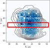 |
Fig. A.1. Simulated slit in the IFU data following the EFOSC2 long-slit observations of S02 marked with a red rectangle. The blueish pixels are those selected to generate the integrated SagDIG spectrum shown in Figure 2, with their respective jump value shown in the colour bar. The black contours represent the Hβ emission line map. |
We found that the reddening corrected emission line measurements of S02 (Table 1 of S02) present a emission line ratio Hγ/Hβ = 0.41±0.11. Hγ/Hβ should be 0.468 under Case B recombination, Te = 10000 K, and Ne = 100 cm−3. This may be produced because S02 perform dust correction with the theoretical ratio Hα/Hβ = 2.85 in the EFOSC2 grism GR#9 spectrum, producing a flux difference for the grism GR#7 spectrum, where the emission lines selected to estimate R23−based metallicities are taken. For this reason, we proceed to perform dust-corrected flux measurements using the Hγ/Hβ = 0.468 theoretical ratio in the EFOSC2 GR#7 spectrum.
To test reliability in the combination between those two spectra for estimating Te−based metallicities, we first compare total oxygen abundances between the mock-slit spectrum and the EFOSC2 spectrum via strong line method R23 (Kobulnicky & Kewley 2004), being the same as used in S02. The R23 index is defined as R23=[I(3727)+I(4959)+I(5007)]/I(Hβ).
We combine the I(3727) measurement from the EFOSC2 long-slit and I(4959)+I(5007) from the VIMOS mock-slit, under the same theoretical ratio to apply dust-correction (Hγ/Hβ = 0.468). The R23 index with this combination is derived as follows:
 (A.1)
(A.1)
On the other hand, R23 index using all the required emission lines from EFOSC2 is estimated with the following expresion:
 (A.2)
(A.2)
So if the derived R23−based metallicities are in agreement between those two ways to estimate R23, we are able to combine the flux measurements to estimate Te−based oxygen abundances, since the combination relies on the flux measurements under the same theoretical value in the dust reddening corrections.
We derived a R23−based oxygen abundance as 12+log(O/H) = 7.30±0.10 using all the required emission line from the EFOSC2 spectrum. Then, using I(3727) form the EFOSC2 and I(4959)+I(5007) from the VIMOS mock-slit, we derived a R23−based oxygen abundance as 12+log(O/H) = 7.31±0.08. Those values are in excellent agreement.
Hence, we proceed to estimate Te for a subsequent derivation of the oxygen abundance using the direct method. We estimate Te[O III] = 22165±1122 K, and Te[O II] = 18515±987. The total oxygen abundances for the VIMOS-mock slit is 12+log(O/H) = 7.23±0.04, and the total oxygen abundance using the EFOSC2 measurements results in 12+log(O/H) = 7.22±0.03. Those estimates are in agreement. The values estimated with this procedure are shown in Table A.1.
Electron temperature and ionic oxygen abundances estimated for SagDIG using Pyneb.
Uncertainties were computed by running 1000 Monte Carlo simulations. We represent each emission line as a random value of a Gaussian distribution centred on the line flux measurement and a standard deviation as the error of the flux measurement.
All Tables
Electron temperature and ionic oxygen abundances estimated for SagDIG using Pyneb.
All Figures
|
Fig. 1. Distribution of jumps for SagDIG H II region spectral fibres shown in blue. The vertical dashed black line indicates the lower limit (25) used to select those fibres in which the integrated spectra of SagDIG H II show the auroral line with S/N > 3. |
| In the text | |
|
Fig. 2. Integrated spectrum of the SagDIG H II region. The left panel shows the window wavelength of the Hγ and [O III]λ4363 emission lines. The middle panel shows the Hβ and [O III]λλ4959,5007 emission lines. The right panel shows the spatial distribution of the selected fibres to generate the integrated spectrum of the SagDIG H II region with auroral detection. The colour code represents the jump value of each selected fibre. The grey contours represent the Hβ emission of the nebula as reference. |
| In the text | |
|
Fig. 3. EFOSC2 long-slit, flux-calibrated 2D frame of the SagDIG H II region. Yellow arrows show the detected emission lines in each slit column. |
| In the text | |
|
Fig. 4. SagDIG H II region emission line maps. The left panel shows the Hβ emission line distribution. The right panel shows the [O III]λ5007 emission line distribution. The colour map represents the flux at each emission line. The dashed grey lines indicate circles of increasing radius of 1.34″ (2 px) up to 12.06″ (18 px). The dotted black lines show the angles that separate the S clump, the NE tail, and the NW clump. |
| In the text | |
|
Fig. 5. Composite image of the flux distribution shown in Figure 4. The blue colour represents the Hβ flux distribution, and the red colour represents the [O III]λ5007 flux distribution. |
| In the text | |
|
Fig. 6. Flux density profiles for the S clump, NW clump, and NE tail structures present in the SagDIG nebula, indicated by black dots, red squares, and blue triangles, respectively. The top panel shows the Hβ flux density profiles. The middle panel shows the [O III]λ5007 flux density profiles. The bottom panel shows the [O III]λ5007 / Hβ flux density profile. |
| In the text | |
|
Fig. 7. Left panel: EFOSC2 pre-imaging frame of the SagDIG H II region. The yellow rectangle shows the slit position used to extract the 2D frame spectra. The vertical yellow lines indicate the area covered by the H II region, from column 280 to column 320. Right panel: 2D frame spectra, where the emission lines detected are indicated by yellow arrows. |
| In the text | |
|
Fig. 8. Emission line ratios across the slit column, representing east-west coordinates in the SagDIG H II region. The upper panel shows the [O III]λ5007/Hβ and the [O III]λ5007/[O II]λ3727 emission line ratios, with green dots and purple squares, respectively. The lower panel shows the [O II]λ3727/Hβ emission line ratio with black dots. |
| In the text | |
|
Fig. 9. Simulated slit in the IFU data following the EFOSC2 long-slit observations of S02 compared to the [O III]λ5007 emission line map indicated by the black contours. The simulated slit was divided into four sections of equal area, where the first and fourth represent the external region in red, and the second and third represent the central region in blue, from left to right, respectively. |
| In the text | |
|
Fig. 10. Comparison of the SagDIG H II region Hβ emission (black contours) with the stellar HST photometry from Momany et al. (2005). The left panel shows the old RGB and red clump stars (white dots) in the H II region. The middle panel shows the distribution of young MS stars (<7 M⊙ and 7−10 M⊙, indicated by cyan dots and cyan crosses, respectively) in the H II region. The orange star is the most luminous (15 M⊙), and the magenta and green crosses are the second and third (>10 M⊙) most luminous stars. The right panel shows the CMD of SagDIG, with the same symbols and colours as in the left and the middle panel. The vertical black curve is a 10 Myr isochrone, showing the MS of young stars to provide a proxy for the stellar masses of the young stars. The horizontal black lines show the corresponding range of masses in the main sequence. |
| In the text | |
|
Fig. 11. HST image (F475W, F606W and F814W combined) acquired by Momany et al. (2005) observations, showing the SagDIG H II region. The left panel shows the location of the old stellar population marked with yellow squares. The right panel shows the young stellar population marked with cyan circles. In both panels, the vertical diffuse column density is indicated with the red arrow. The source in the upper right region is a foreground star. |
| In the text | |
|
Fig. 12. SagDIG in the mass-metallicity plane marked with a white triangle and white dots for the Te corrected and uncorrected oxygen abundance, respectively. The dotted black and solid blue lines are the local Universe Te−based MZR of Curti et al. (2020) and Andrews & Martini (2013). The black and solid red lines represent the low-mass end of the MZR from Lee et al. (2006) and Berg et al. (2012). The contours represent the respective galaxy sample of dIrr galaxies used to fit the low-mass end of the MZR marked with corresponding colours. The dashed red area indicates the respective scatter of σ = 0.15 dex of the Berg et al. (2012) low-mass end of the MZR. |
| In the text | |
|
Fig. A.1. Simulated slit in the IFU data following the EFOSC2 long-slit observations of S02 marked with a red rectangle. The blueish pixels are those selected to generate the integrated SagDIG spectrum shown in Figure 2, with their respective jump value shown in the colour bar. The black contours represent the Hβ emission line map. |
| In the text | |
Current usage metrics show cumulative count of Article Views (full-text article views including HTML views, PDF and ePub downloads, according to the available data) and Abstracts Views on Vision4Press platform.
Data correspond to usage on the plateform after 2015. The current usage metrics is available 48-96 hours after online publication and is updated daily on week days.
Initial download of the metrics may take a while.