© The Authors 2025

1 Introduction

Knowledge of the interior structure of Venus is needed to understand its history and to gather insights into why its evolutionary path diverged so significantly from that of Earth. Magellan, the most recent mission to Venus with a specific focus on its interior, enabled measurements of its gravity field (Konopliv et al. 1999) and tidal deformations (Konopliv & Yoder 1996), but lacked the precision needed to determine the state of the core (Dumoulin et al. 2017). Current plausible interior models for Venus consider a core that can be entirely liquid, entirely solid, or composed of a liquid outer core with a solid inner core (Dumoulin et al. 2017; Shah et al. 2022; Saliby et al. 2023).

Examining an object’s rotational dynamics can offer clues about the nature and properties of its interior. The motion of a planet’s spin axis can be described relative to the fixed celestial sphere (precession and nutation) or relative to the planetary surface itself (polar motion). Both motions bring complementary constraints for interior models. Venus’s spin axis precession was first measured by Margot et al. (2021) using ground-based observations, providing an estimate of its moment of inertia which imposed loose constraints on the size of the core. This is a powerful technique, as it measures the orientation of a planet’s spin axis in inertial space without requiring direct observation of the planetary surface. However, as a consequence, it did not measure the orientation of the spin pole relative to the surface.

The free component of a planet’s polar motion is directly linked to its internal properties. On Earth, it was first measured by Chandler (1891) and has since been named the “Chandler wobble”. Among the other planets, this free motion has only been detected on Mars (Konopliv et al. 2020), which allowed to constrain the mantle rheology at a larger period than other tidal periods. Polar motions of the proto-planets (1) Ceres and (2) Vesta have been computed in perspective of the Dawn mission, but were not detected (Rambaux et al. 2011; Rambaux 2013). During the early Pioneer Venus Orbiter mission, Yoder & Ward (1979) studied the hypothesized Chandler wobble of Venus, focusing on its amplitude (i.e., the angle between the spin axis and the polar principal axis of inertia), but that angle could not be measured. Since a non-zero amplitude is not a stable state, they explored the potential value of this amplitude by characterizing the wobble excitation and estimating its damping efficiency. Based on the degree-2 gravity field obtained later by the Magellan mission, this angle was measured at 0.5° (Konopliv et al. 1999). The mechanisms that could excite Venus’s polar motion to that amplitude are still not fully understood, although mantle convection has been studied as a potential excitation source (e.g., Spada et al. 1996). Measuring the period of Venus’s Chandler wobble, which offers a direct link to the planet’s interior, requires detecting the motion of its spin pole, rather than solely measuring its position.

With a spacecraft in orbit around Venus, signals of its precession and polar motion could be detected by tracking surface radar features, or through the gravitational effect of spin dynamics on the spacecraft trajectory. The Magellan mission lacked the precision to detect these signals with either approach, but the detection of the precession has already been simulated for upcoming missions (Rosenblatt et al. 2021; Cascioli et al. 2021). However, detecting Venus’s polar motion has not yet been addressed with similar analyses.

As a step toward this goal, we present a complete model for Venus’s polar motion, by determining its relationship with the planet’s interior and its atmospheric dynamics. In this work, Venus is modeled with a spherical core, a solid deformable triaxial mantle, and a fluid atmosphere. In Sect. 2, we describe the framework used to study the dynamics of the spin axis of Venus’s mantle in a body-fixed reference frame: the Euler-Liouville equation, which forms the basis of our derivation of polar motion, and the relevant physical phenomena; namely, the solar torque, solid deformations, and atmospheric dynamics. Their individual effects on polar motion are presented in Sect. 3, where we characterize the Chandler period and damping time, and the forced polar motion, as applied to Venus. In Sect. 4.2, we discuss the impact of different assumptions for core-mantle dynamical coupling and how they relate to the physical state of the core. Then, applications of the polar motion model to Venus, Earth and Mars are compared in Sect. 4.3. Finally, in Sect. 4.4, we discuss the potential for future missions, focusing on EnVision, to detect and measure Venus’s polar motion. We also discuss the constraints this could provide on Venus’s internal structure.

2 Polar motion model

2.1 Linearized Euler-Liouville equation

We analyzed the polar motion of Venus, defined as the motion of its spin axis in a body-fixed frame, via the Euler rotation equation. It describes the dynamics of angular momentum H in a non-inertial reference frame with $$\dot{H}+\omega \times H=\mathrm{\Gamma },$$(1)

where ω is the instantaneous rotation vector of that reference frame and Γ is the external torque. The polar motion is obtained by solving this equation for ω in a Venus body-fixed frame, such that ω also describes the rotation of the planet (Munk & MacDonald 1960; Gross 2015; Rambaux 2013).

We worked in the body-fixed frame in which the time-averaged inertia matrix, I₀, is diagonal, referred to as the body reference frame (BRF), whose axes are the principal axes of inertia of the planet. In this reference frame, Venus’s spin axis remains close to the z-axis (with a present-day angle of 0.481° ± 0.020°, Konopliv et al. 1999), so the rotation vector can then be written as variations, Δω, to the main z-axis component, ω₀: $$\omega ={\omega }_0+\mathrm{\Delta }\omega =\left(\begin{array}{c}0\\ 0\\ \mathrm{\Omega }\end{array}\right)+\mathrm{\Omega }\left(\begin{array}{c}{m}_x\\ m_y\\ m_z\end{array}\right),$$(2)

where Ω is the constant mean rotation rate of Venus, and m_x, m_y, and m_z are treated as small quantities. In this work, the retrograde rotation of Venus appears as a negative Ω, with an obliquity that is between 0° and 90° (ε = 2.6392° ± 0.0008°, Margot et al. 2021), but switching to the opposite convention does not affect the results. The values of parameters used for Venus in this work are listed in Table A.1.

To solve Eq. (1) for ω we express the angular momentum as $$H=\mathcal{I}\omega +h,$$(3)

where I is the inertia matrix of the planet including the atmosphere, so that Iω represents the angular momentum of a uniformly rotating planet including an atmosphere at rest. The winds contribute additional angular momentum, h. When written in the BRF, the inertia matrix, I, is decomposed into a mean term, I₀, and the small deformation term ΔI originating from both mantle and atmospheric deformation, with $$\mathcal{I}={\mathcal{I}}_0+\mathrm{\Delta }\mathcal{I}=\left[\begin{array}{ccc}A& 0& 0\\ 0& B& 0\\ 0& 0& C\end{array}\right]+\left[\begin{array}{ccc}\mathrm{\Delta }{\mathcal{I}}_{xx}& \mathrm{\Delta }{\mathcal{I}}_{xy}& \mathrm{\Delta }{\mathcal{I}}_{xz}\\ \mathrm{\Delta }{\mathcal{I}}_{xy}& \mathrm{\Delta }{\mathcal{I}}_{yy}& \mathrm{\Delta }{\mathcal{I}}_{yz}\\ \mathrm{\Delta }{\mathcal{I}}_{xz}& \mathrm{\Delta }{\mathcal{I}}_{yz}& \mathrm{\Delta }{\mathcal{I}}_{zz}\end{array}\right].$$(4)

In this work, the mean moments of inertia (A, B, C) are either those of the whole planet (core, mantle and atmosphere) if the core is assumed to be dynamically locked with the mantle; or those without the core, if it is decoupled from the mantle (see Sect. 4.2).

As is the case for Venus, the atmosphere is in a state of global super-rotation when the excess angular momentum h from the winds has a non-zero average. Here, this excess angular momentum is assumed to have constant amplitude and to take place around the planet’s spin axis. It is noted h_sr, and the small variations from atmospheric dynamics are denoted as Δh : $$h=h_{sr}+\mathrm{\Delta }h=k\omega +\left(\begin{array}{c}\mathrm{\Delta }{h}_x\\ \mathrm{\Delta }{h}_y\\ \mathrm{\Delta }{h}_z\end{array}\right),$$(5)

where k is the scalar coefficient between hsr and ω. In the absence of super-rotation, k = 0. For Venus, k/C ≈ 10⁻³ (see Sect. 4.1). With a first-order expansion in small quantities, the effects of atmosphere super-rotation are too minor to be taken into account here. Still, in Sect. 4.1 we retain the terms with k to discuss how super-rotation affects polar motion.

Using Eqs. (2)-(4) in Eq. (1), and keeping only the first-order terms in Δω, ΔI and h, we have the Euler-Liouville equations (e.g., Munk & MacDonald 1960, Chap. 6): $$\begin{gathered} A\dot{m_x}+\dot{\mathrm{\Delta }{\mathcal{I}}_{xz}}+\frac{1}{\mathrm{\Omega }}\dot{\mathrm{\Delta }{h}_x}+\mathrm{\Omega }(C-B)m_y-\mathrm{\Omega }\mathrm{\Delta }{\mathcal{I}}_{yz}-\mathrm{\Delta }{h}_y=\frac{1}{\mathrm{\Omega }}{\mathrm{\Gamma }}_x \\ B\dot{m_y}+\dot{\mathrm{\Delta }{\mathcal{I}}_{yz}}+\frac{1}{\mathrm{\Omega }}\dot{\mathrm{\Delta }{h}_y}-\mathrm{\Omega }(C-A)m_x+\mathrm{\Omega }\mathrm{\Delta }{\mathcal{I}}_{xz}+\mathrm{\Delta }{h}_x=\frac{1}{\mathrm{\Omega }}{\mathrm{\Gamma }}_y \\ C\dot{m_z}+\dot{\mathrm{\Delta }{\mathcal{I}}_{zz}}+\frac{1}{\mathrm{\Omega }}\dot{\mathrm{\Delta }{h}_z}=\frac{1}{\mathrm{\Omega }}{\mathrm{\Gamma }}_z. \end{gathered}$$(6)

The third dimension is now decoupled from the others and can be studied separately to analyze m_z, the spin rate variations (Cottereau et al. 2011). The polar motion is described by m_x and m_y, the projection of the unit rotation vector onto the equatorial plane of the BRF. The first two dimensions of Eq. (6) are combined into a single complex equation by introducing the following complex notations: m = m_x + im_y, T = Γ_x + iΓ_y, ΔI = ΔI_xz + iΔΙ_yz, and Δh = Δh_x + iΔ h_y. This yields $$\begin{gathered} [\frac{A+B}{2}\dot{m}-i\mathrm{\Omega }(C-\frac{A+B}{2})m]-\frac{B-A}{2}(\dot{\overline{m}}+i\mathrm{\Omega }\overline{m}) \\ =\frac{1}{\mathrm{\Omega }}T-(i\mathrm{\Omega }\mathrm{\Delta }I+\dot{\mathrm{\Delta }I})-(i\mathrm{\Delta }h+\frac{1}{\mathrm{\Omega }}\dot{\mathrm{\Delta }h}), \end{gathered}$$(7)

where m̄ is the complex conjugate of m.

The Chandler wobble is the free oscillation that can be characterized by solving the homogeneous equation from Eq. (7) for m, effectively ignoring the terms that are periodic with external forcing periods. However, some terms on the right-hand side of the equation depend on m, thus affecting the homogeneous system. They need to be identified for a complete description of the Chandler wobble. For instance, the solid rotational deformation term is proportional to m, lengthening the Earth’s calculated wobble period by 38% (e.g., Gross 2015). As pointed out by Baland et al. (2019, Appendix 2), the solar torque term for a rigid planet also contains components proportional to m, but shortens the Earth’s free wobble period by less than 0.001%. In the sections below, we explore how these m-dependent terms affect Venus’s free wobble.

2.2 Solar torque influence on the rigid Chandler wobble

Here, we highlight how the solar torque affects the wobble by considering a simplified non-deformable solid body without relative atmospheric angular momentum, thus ignoring the terms in ΔI and h. Venus’s orbit currently has an eccentricity of 0.0067, the lowest among Solar System planets; hence, our analysis assumes a circular orbit.

The solar torque exerted on Venus depends on the position r of the Sun and on Venus’s inertia matrix, both expressed in the BRF. It can be written like in Williams et al. (2001) as $$\mathrm{\Gamma }=3\frac{G{M}_{\odot }}{\Vert r{\Vert }^5}r\times \mathcal{I}r,$$(8)

where G is the gravitational constant and M the mass of the Sun. By neglecting the deformations and the eccentricity, we find the complex representation of the torque: $$T_0=3n^2[(C-\frac{A+B}{2})(yz-ixz)-\frac{B-A}{2}(yz+ixz)],$$(9)

with n the mean orbital motion of Venus, and $r/\Vert r\Vert =(x,y,z{)}^T$ in the BRF. Then, to solve Eq. (7), we need to derive analytical expressions for the products yz and xz.

We define an orbital reference frame (ORF) centered on Venus. Its xy-plane coincides with Venus’s orbital plane, and the ascending node of this plane on the ICRF equator defines the ORF x-axis. In this work, the effects of other planets on Venus’s orbit are neglected, allowing the ORF to be considered an inertial reference frame. For a circular orbit, with M = nt + M₀ the mean anomaly of Venus, the planet’s coordinates in its own orbital plane are given by $\Vert r\Vert (\cos M,\sin M,0{)}^T={\mathcal{R}}_z(-M)(\Vert r\Vert ,0,0{)}^T$, using the elementary rotation matrices: $${\mathcal{R}}_z(\theta )=\left[\begin{array}{ccc}\cos \theta & \sin \theta & 0\\ -\sin \theta & \cos \theta & 0\\ 0& 0& 1\end{array}\right]\text{\hspace{0.17em}and\hspace{0.17em}}{\mathcal{R}}_x(\theta )=\left[\begin{array}{ccc}1& 0& 0\\ 0& \cos \theta & \sin \theta \\ 0& -\sin \theta & \cos \theta \end{array}\right].$$(10)

The coordinates of the Sun in the ORF, centered on Venus, are given by the opposite vector $$\frac{r_{\mathrm{O}\mathrm{R}\mathrm{F}}}{\Vert r\Vert }=-\left(\begin{array}{c}\cos M\\ \sin M\\ 0\end{array}\right)=-{\mathcal{R}}_z(-M)\left(\begin{array}{c}1\\ 0\\ 0\end{array}\right).$$(11)

To obtain the coordinates of the Sun in the BRF, we use an intermediate rotating frame, referred to as the spin reference frame (SRF), whose z-axis coincides with the spin axis ω, and whose x-axis points toward Venus’s prime meridian. The transformation from the ORF to the SRF is described with Euler angles, as illustrated in Fig. 1: $$r_{\mathrm{S}\mathrm{R}\mathrm{F}}={\mathcal{R}}_z(\varphi ){\mathcal{R}}_x(ϵ){\mathcal{R}}_z(\psi )r_{\mathrm{O}\mathrm{R}\mathrm{F}}.$$(12)

Here, ε is the obliquity of Venus, φ = Ωt + φ₀ is the rotation angle of its prime meridian, and ψ is the longitude of the ascending node of Venus’s equator on its orbital plane (i.e., the nodal precession angle).

Due to the non-zero polar motion, the SRF is not a body-fixed reference frame. When the inertia matrix of Venus is expressed in the SRF, its eigenvectors make up the rows of the matrix transformation from the SRF to the BRF, which we describe with Euler angles (α, β, γ): $$r_{\mathrm{B}\mathrm{R}\mathrm{F}}={\mathcal{R}}_z(\alpha ){\mathcal{R}}_x(\beta ){\mathcal{R}}_z(\gamma )r_{\mathrm{S}\mathrm{R}\mathrm{F}}.$$(13)

They can be derived from a set of degree-2 gravity coefficients that uses the SRF, as in Konopliv et al. (1999), and the values of (α, β, γ) for Venus at epoch J2000 are given in Table A.1. Here, β is the angle between the spin axis and the polar principal axis of inertia (i.e., the amplitude of polar motion). Both angles α and γ evolve with the phase of polar motion, with α increasing and γ decreasing in the case of Venus. The configuration depicted in Fig. 1 is similar to that at epoch J2000, where α_J2000 is positive and γ_J2000 is negative. The sum α + γ represents the longitudinal offset between the smallest principal axis of inertia of Venus and its prime meridian, measured at −3.17° (Konopliv et al. 1999).

Using Eqs. (11)-(13), we have a complete representation of the coordinates of the Sun in the BRF: $$\frac{r_{BRF}}{\Vert r\Vert }=-{\mathcal{R}}_z(\alpha ){\mathcal{R}}_x(\beta ){\mathcal{R}}_z(\gamma ){\mathcal{R}}_z(\varphi ){\mathcal{R}}_x(ϵ){\mathcal{R}}_z(\psi ){\mathcal{R}}_z(-M)\left(\begin{array}{c}1\\ 0\\ 0\end{array}\right)$$(14) $$\frac{r_{BRF}}{\Vert r\Vert }=\left(\begin{array}{c}x\\ y\\ z\end{array}\right)=\left(\begin{array}{c}-\cos ((M-\varphi )-(\psi +\gamma +\alpha ))\\ -\sin ((M-\varphi )-(\psi +\gamma +\alpha ))\\ ϵ\sin (M-\psi )+\beta \sin ((M-\varphi )-(\psi +\gamma ))\end{array}\right),$$(15)

where we considered only the first-order terms in ε and β. Here M and φ are the fast-rotating angles, with respectively a 224.7 days orbital period and a −243.0 days rotation period. The other angles are much slower, namely, the precession angle ψ has a ≈29 000 years period (Margot et al. 2021), and both −α and γ have periods corresponding to the Chandler period which we find to be ≈16 000 years. The products xz and yz are found to contain terms with the three fast angles θ_j defined in Table 1, but also contain a term with the angle α: $$\begin{gathered} xz=\frac{ϵ}{2}(\sin {\theta }_1-\sin {\theta }_2)-\frac{\beta }{2}(\sin {\theta }_3+\sin \alpha ) \\ yz=-\frac{ϵ}{2}(\cos {\theta }_1-\cos {\theta }_2)+\frac{\beta }{2}(\cos {\theta }_3-\cos \alpha ) \\ xy=\frac{1}{2}\sin ({\theta }_3-\alpha ). \end{gathered}$$(16)

Moreover, from the definition of both reference frames we have: ${\omega }_{\mathrm{B}\mathrm{R}\mathrm{F}}=\mathrm{\Omega }(m_x,m_y,1+m_z{)}^T$ and ${\omega }_{\mathrm{S}\mathrm{R}\mathrm{F}}=\mathrm{\Omega }(0,0,1{)}^T$. Hence, the Euler angles α and β, involved in the transformation Eq. (13) describing the polar motion, are linked to m_x and m_y with $$m=m_x+i{m}_y=\beta (\sin \alpha +i\cos \alpha )=i\beta e^{-i\alpha }.$$(17)

The torque Eq. (9) is thus found to be $$\begin{gathered} T_0=i\frac{3}{2}{n}^2[(C-\frac{A+B}{2})m+\frac{B-A}{2}\overline{m}] \\ +\frac{3}{2}{n}^2(C-\frac{A+B}{2})[ϵ(-e^{i{\theta }_1}+e^{i{\theta }_2})+\beta e^{i{\theta }_3}] \\ +\frac{3}{2}{n}^2\frac{B-A}{2}[ϵ(e^{-i{\theta }_1}-e^{-i{\theta }_2})-\beta e^{-i{\theta }_3}]. \end{gathered}$$(18)

The components in θ_j, in the last two lines, contain the fast angles. Thus, they are unrelated to the Chandler wobble and treated as forcing terms, as described in Sect. 3.2.

On the other hand, the terms in the first line are proportional to m and m̄; we substitute these terms in the Euler Equation (7): $$\begin{gathered} [\frac{A+B}{2}\dot{m}-i\mathrm{\Omega }(C-\frac{A+B}{2})m]-\frac{B-A}{2}(\dot{\overline{m}}+i\mathrm{\Omega }\overline{m}) \\ -i\frac{3}{2}\frac{n^2}{\mathrm{\Omega }}[(C-\frac{A+B}{2})m+\frac{B-A}{2}\overline{m}]=0. \end{gathered}$$(19)

It lets us find the free rigid Chandler wobble solution: $$m(t)=m_0\exp (i{\sigma }_{r}t)-\frac{\kappa -1}{\kappa +1}\overline{m_0}\exp (-i{\sigma }_{r}t),$$(20)

which can be written as $$\begin{gathered} m_x(t)=m_{x0}\cos ({\sigma }_{r}t+\eta ) \\ {m}_y(t)=\kappa m_{x0}\sin ({\sigma }_{r}t+\eta ), \end{gathered}$$(21)

with the frequency and the ellipticity of the wobble being $${\sigma }_r=\mathrm{\Omega }\sqrt{\frac{C-A}{A}\frac{C-B}{B}}(1+\frac{3}{2}\frac{n^2}{{\mathrm{\Omega }}^2}),$$(22) $$\kappa =\sqrt{\frac{C-A}{C-B}\frac{A}{B}},$$(23)

and where the complex initial condition m₀ , or the real ones (m_x0, η), must be constrained by observations. The triaxiality of the planet results in an elliptic motion as shown in Fig. 3, with κ > 1, and with the presence of the negative Chandler frequency in Eq. (20). As previously discussed, the values to use for (A, B, C) should either be those of the whole planet (core, mantle and atmosphere) or those without the core, depending on the core-mantle coupling assumption.

Equation (22) for the Chandler frequency accounts for the solar torque, aligning with the expressions already obtained by Yoder (1997) and Baland et al. (2019, Appendix 2), while also accounting for triaxiality as done in Rambaux (2013). In Sect. 2.3, we extend it to incorporate the effects of solid deformation. The key point here is that the solar torque, usually ignored when studying the free Chandler wobble, actually increases the Chandler frequency by a factor of 1 + (3n²)/(2Ω²), which is about 2.75 when applied to Venus. For Earth and Mars, which rotate faster, this factor has respective values of (1 + 10⁻⁵) and (1 + 3 × 10⁻⁶) and can be considered negligible. Another way to understand the contribution of the solar torque is to develop the Chandler frequency Eq. (22) as $${\sigma }_r=\mathrm{\Omega }\sqrt{\frac{C-A}{A}\frac{C-B}{B}}+q\frac{3}{2}\frac{n^2}{\mathrm{\Omega }}\frac{C-\frac{A+B}{2}}{C},$$(24)

where $q=\frac{C}{\sqrt{AB}}\frac{2\sqrt{(C-A)(C-B)}}{(C-A)+(C-B)}$ accounts for the non-sphericity of the planet, and is close to 1. The first term is the usual formulation of the Chandler frequency which ignores the solar torque (e.g., Rambaux 2013; Konopliv et al. 2020). Neglecting triaxiality (q = 1) and assuming a small obliquity, we recognize in the second term the frequency of the precession due to solar torque (e.g., Williams 1994). Comparing the two terms of Eq. (24), in the cases of Earth and Mars, the torque-free wobble has a relatively high frequency (on the order of a few hundred days) compared to that of the solar-induced precession, which is on the order of a hundred thousand years, making the second term negligible. In the case of Venus, the torque-free wobble and solar-induced precession have periods of the same order, respectively, ≈51000 years and ≈29 000 years, so both terms in Eq. (24) should be kept, resulting in a Chandler wobble period shorter than both.

The expression in Eq. (22) for the Chandler frequency, σ_r, is valid for a non-deformable solid body, where ignoring the dissipative processes leads to the absence of damping for the Chandler wobble. In the next section, we introduce solid deformation into the model.

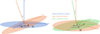Fig. 1 Transformations between the ORF (blue), SRF (orange), and BRF (green), with Euler angles. The SRF and the BRF are both rotating frames, with ZS the spin axis of Venus and ZB its polar principal axis. The polar motion is the relative motion between the SRF and the BRF.

2.3 Solid deformations

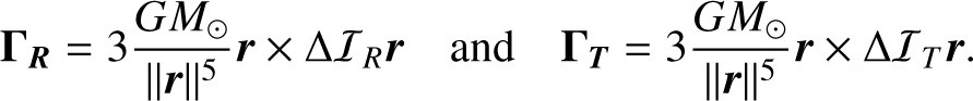
The solid viscoelastic deformation of Venus’s solid body affects polar motion in two distinct ways. A direct effect is due to angular momentum conservation and is seen in Eq. (7) with the terms in ΔI and its derivative; and indirectly, variations of I can induce variations in the net solar torque, as shown in Eq. (8). Here, we explore two sources of solid deformation for Venus: the centrifugal potential and the solar tidal potential, which cause variations ΔI_R and ΔI_T of the inertia matrix. They result in additional torque terms, respectively Γ_R and Γ_T. All of these terms are taken into account in Eq. (7) with ΔI = ΔIR + ΔIT and T=T +T +T.

2.3.1 Love numbers formalism

The tidal response ΔI of a body to a perturbation ΔI^p depends on the history of said perturbation: $\mathrm{\Delta }{\mathcal{I}}^p$, where the symbol * designates the temporal convolution, and $\widetilde{k_2}(\tau )$ is a convolution kernel that depends on the rheology of the body (e.g., Boué et al. 2016; Correia & Valente 2022).

In practice, when the excitation is decomposed as a set of distinct periodic components, it means that components of different frequencies ν_j are affected by different Love numbers $k_2^{(j)}$, which come from the Fourier transform of $\widetilde{k_2}(\tau )$. These Love numbers have complex values $k_2^{(j)}=|k_2^{(j)}|\exp (i{\delta }_j)$, where the modules $|k_2^{(j)}|$ are the amplitude gains of Venus’s response, and the arguments δ_j are the phase lags that characterize the inelastic response. Here, in equations where an excitation term contains multiple periodic components, we use the convolution notation for improved clarity. When the components are developed separately, we use the individual $k_2^{(j)}$ values.

To date, the tidal response of Venus has only been measured at the semi-diurnal period of 58 days (Konopliv & Yoder 1996) and rheological models are needed to extrapolate this data to other frequencies. We use models provided by Musseau et al. (2024), where some have a constant mantle viscosity, ranging from 10¹⁹ Pas to 10²² Pa s, and some have a viscosity profile which they fitted to match the current rotation rate of Venus, where the thermal atmospheric tides compensate the solid tides to an equilibrium. The $|k_2^{(j)}|$ and δ_j values from their four-layer viscosity profile and V5-T_hot interior model are given in Table 1.

Here, we use the convention that for positive frequencies δ_j is negative, whereas for negative frequencies, δ_j is positive.

2.3.2 Centrifugal and tidal deformations

We derive the centrifugal deformation ΔI_R caused by Venus’s rotation and the tidal deformation ΔI_T caused by the gravity of the Sun. We followed the expressions of Williams et al. (2001) where we removed the average components, already contained in I₀, and retained only the first-order terms in β and ε. It leads to the following expressions: $$\begin{gathered} \mathrm{\Delta }{\mathcal{I}}_R=\widetilde{k_2}\ast \frac{{\mathrm{\Omega }}^2{R}^5}{3G}\left[\begin{array}{c}-\frac{2}{3}{m}_{z}0m_x\\ 0-\frac{2}{3}{m}_z{m}_y\\ m_x{m}_y\frac{4}{3}{m}_z\end{array}\right], \\ \mathrm{\Delta }{\mathcal{I}}_T=-\widetilde{k_2}\ast \frac{n^2{R}^5}{G}\left[\begin{array}{c}{x}^2-\frac{1}{2}xyxz\\ xy{y}^2-\frac{1}{2}yz\\ xzyz0\end{array}\right], \end{gathered}$$(25)

where R is the mean radius of Venus, and $\widetilde{k_2}$ encompasses the response of Venus’s gravitational potential to a perturbation potential. With Eq. (16), we can express their complex representations with only the terms from their third column, $\mathrm{\Delta }I=\mathrm{\Delta }{\mathcal{I}}_{xz}+i\mathrm{\Delta }{\mathcal{I}}_{yz}$: $$\begin{gathered} \mathrm{\Delta }{I}_R=k_2^{(\mathrm{c}\mathrm{w})}\frac{{\mathrm{\Omega }}^2{R}^5}{3G}m, \\ \mathrm{\Delta }{I}_T=k_2^{(\mathrm{c}\mathrm{w})}\frac{n^2{R}^5}{2G}m+i\frac{n^2{R}^5}{2G}[ϵ(k_2^{(1)}{e}^{i{\theta }_1}-k_2^{(2)}{e}^{i{\theta }_2})-\beta k_2^{(3)}{e}^{i{\theta }_3}]. \end{gathered}$$(26)

We find that ΔI_R is entirely proportional to m, whereas ΔI_T combines a term proportional to m along with three terms with fast forcing frequencies.

2.3.3 Additional torque on the deformations

The additional solar torque terms that arise from the deformations terms ΔI_R and ΔI_T are $${\mathrm{\Gamma }}_R=3\frac{G{M}_{\odot }}{\Vert r{\Vert }^5}r\times \mathrm{\Delta }{\mathcal{I}}_{R}r\text{and}{\mathrm{\Gamma }}_T=3\frac{G{M}_{\odot }}{\Vert r{\Vert }^5}r\times \mathrm{\Delta }{\mathcal{I}}_{T}r.$$(27)

Plugging in the matrices of Eq. (25), with a careful handling of the frequency dependence of the k₂ Love number (see Appendix B), we find $$T_R=-i{k}_2^{(\mathrm{c}\mathrm{w})}\frac{n^2{\mathrm{\Omega }}^2{R}^5}{2G}m-\overline{k_2^{(\mathrm{c}\mathrm{w})}}\beta \frac{n^2{\mathrm{\Omega }}^2{R}^5}{2G}{e}^{i{\theta }_3},$$(28) $$\begin{gathered} T_T=-i\frac{3}{4}\frac{n^4{R}^5}{G}(k_2^{(\mathrm{c}\mathrm{w})}+\overline{k_2^{(3)}}-k_2^{(3)})m+\frac{3}{4}\frac{n^4{R}^5}{G}[-\overline{k_2^{(\mathrm{c}\mathrm{w})}}\beta e^{i{\theta }_3} \\ +(k_2^{(1)}+\overline{k_2^{(2)}}-k_2^{(3)})ϵe^{i{\theta }_1}-(\overline{k_2^{(1)}}+k_2^{(2)}-k_2^{(3)})ϵe^{i{\theta }_2}]. \end{gathered}$$(29)

The terms proportional to m from ΔI_R, ΔI_T, TR and T_R, from Eqs. (26), (28), and (29), must be taken into account along with those from Eq. (18) to fully characterize the free response. This will be achieved in Sect. 3.1.

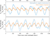Fig. 2 X and Y equatorial components of the atmospheric relative angular momentum (Δha, blue) and of the polar motion it induces on the solid body (ma, orange). The angular momentum is normalized by |CΩ| which is the transfer function for high frequencies. Bright lines show the numerical time series for the Δha, with ma computed through a Discrete Fourier Transform. Darker lines show the quasi-periodic approximation for Δha with only the first three components of Table 2, with ma computed analytically. The time axis is in Earth days.

2.4 Atmospheric forcing

The atmosphere of Venus affects its solid body spin dynamics through pressure and friction forces on the surface, resulting in a net torque exerted on the solid body. Here, we consider the system composed of the solid planet and the atmosphere, so this forcing is no longer seen as an external torque. Instead, the interaction is controlled by the conservation of total angular momentum. The effect on polar motion appears in Eq. (7), where winds vary the angular momentum vector of the atmosphere and mass motions vary its inertia matrix.

The Venus Planetary Climate Model (V-PCM) reproduces atmospheric dynamics (Lebonnois et al. 2010; Lai et al. 2024), by simulating physical, chemical and radiative processes within a 3D grid. Of particular interest here, it computes for each cell the zonal and meridional wind velocities (u and v, respectively) along with the density ρ, which all contribute to the angular momentum and inertia of the whole atmosphere. The simulation run by Lai et al. (2024) provides us with an uninterrupted time series spanning 20 Venus solar days - more than 6 Earth years. They simulated the dynamics with 240 time steps per Venus solar day, in a grid of 145 latitudes, 288 longitudes, and 50 vertical levels. Closer to the surface, the levels become progressively thinner and follow the topography, providing a finer vertical resolution in the deep atmosphere.

The wind and density quantities contribute to the terms h and ΔI, when spatially integrated over the longitude, λ, the latitude, μ, and the radius, r : $$\begin{gathered} h_{a,x}={\int }_{V}r(u\cos \lambda \sin \mu +v\sin \lambda )dm \\ {h}_{a,y}={\int }_{V}r(u\sin \lambda \sin \mu -v\cos \lambda )dm \\ {h}_{a,z}={\int }_{V}r(-u\cos \mu )dm, \end{gathered}$$(30) $$\begin{gathered} \mathrm{\Delta }{\mathcal{I}}_{a,xz}={\int }_V{r}^2\cos \lambda \cos \mu \sin \mu dm \\ \mathrm{\Delta }{\mathcal{I}}_{a,yz}={\int }_V{r}^2\sin \lambda \cos \mu \sin \mu dm \\ \mathrm{\Delta }{\mathcal{I}}_{a,zz}={\int }_V{r}^2{\cos }^2\mu dm, \end{gathered}$$(31)

where dm = ρr² cosμ dr dμ dλ, and taking u positive when westward and v positive when northward. This is similar to the approach of Dehant et al. (2005), but we integrate vertically using the distance coordinate rather than the pressure coordinate. Here, Eqs. (30) and (31) use longitudes and latitudes given in the V-PCM coordinate system, attached to the SRF defined in Sect. 2.2.

We obtain time series for h_a and ΔI_a, from which we determine h_sr, and Δh_a = ha - h_sr. The resulting polar motion response can be computed through the transfer function determined in Sect. 3.2, using a Discrete Fourier Transform. Additionally, to provide greater interpretability of individual frequency contributions, we approximate each complex-valued time series as a finite sum of periodic components: $$\mathrm{\Delta }{h}_a=\sum _k\mathrm{\Delta }{h}_k{e}^{i{\nu }_{k}t}\text{and}\mathrm{\Delta }{I}_a=\sum _k\mathrm{\Delta }{I}_k{e}^{i{\nu }_{k}t},$$(32)

with the process described by Laskar (1993), implemented in the frequency analysis tools provided by TRIP (Gastineau & Laskar 2011).

Figure 2 shows the numerical series for the equatorial angular momentum Δh_a, along with its analytical approximation consisting of the first three frequency components listed in Table 2. The main periodicity is found to be at 243.42 days, closely matching Venus’s sidereal rotation period, and the next significant components match the solar day of 116.75 days. The effect of the atmospheric inertia variations ΔI_a on polar motion is three orders of magnitude smaller that of Δh_a; the frequencies and amplitudes recovered for ΔI_a are nonetheless listed in Table 3.

Excitation functions in the right-hand side of Eq. (7) can also be written as sums of periodic components: $$\begin{gathered} i\mathrm{\Delta }{h}_a+\frac{1}{\mathrm{\Omega }}\dot{\mathrm{\Delta }{h}_a}=i\sum _k(1+\frac{{\nu }_k}{\mathrm{\Omega }})\mathrm{\Delta }{h}_k{e}^{i{\nu }_{k}t}, \\ i\mathrm{\Omega }\mathrm{\Delta }{I}_a+\dot{\mathrm{\Delta }{I}_a}=i\sum _k(\mathrm{\Omega }+{\nu }_k)\mathrm{\Delta }{I}_k{e}^{i{\nu }_{k}t}. \end{gathered}$$(33)

These excitation terms, along with those from T₀, ΔI_T, T_R and TT in Eqs. (18), (26), (28), and (29), excite the polar motion, whose forced response computation is described in Sect. 3.2.

3 Polar motion solution for Venus

Here, we analytically characterize the period and damping time of Venus’s Chandler wobble in Sect. 3.1, as well as the amplitudes and phases of the forced polar motion response in Sect. 3.2.

The terms not associated with forcing (i.e., those depending on m rather than on forcing frequencies) from the expressions of (i) the solar torque on the mean figure of Venus Eq. (18); (ii) the centrifugal and tidal deformations Eq. (26); and (iii) the solar torque exerted on these deformations Eqs. (28), (29), are all gathered on the left-hand side of Eq. (7). The forcing terms are kept on the right-hand side, as a sum of periodic terms. We use the following notations: $$s=1+\frac{3}{2}\frac{n^2}{{\mathrm{\Omega }}^2},D=k_2^{(\mathrm{c}\mathrm{w})}\frac{{\mathrm{\Omega }}^2{R}^5}{3G},$$(34) $$\text{and}{D}^{\prime }=-i\mathrm{I}\mathrm{m}[{\mathrm{k}}_2^{(3)}]\frac{\mathrm{s}-1}{\mathrm{s}}\frac{{\mathrm{n}}^2{\mathrm{R}}^5}{\mathrm{G}},$$(35)

where s is the factor already encountered in Eq. (22) and D is a complex deformation term homogeneous to a moment of inertia having the same phase δ_cw as $k_2^{(\mathrm{c}\mathrm{w})}$. D′ involves the dissipation at the semi-diurnal tide (58 days). We obtain $$\begin{gathered} (\frac{A+B}{2}+sD)\dot{m}-i\mathrm{\Omega }s(C-\frac{A+B}{2}-sD-D^{\prime })m \\ -\frac{B-A}{2}(\dot{\overline{m}}+i\mathrm{\Omega }s\overline{m})=\sum _k{F}_k{e}^{i{\nu }_{k}t}. \end{gathered}$$(36)

3.1 Chandler wobble

The free solution to Eq. (36) has an expression similar to the rigid case solution: $$m(t)=m_0\exp (i{\alpha }_{\mathrm{c}\mathrm{w}}t)-\frac{\kappa -1}{\kappa +1}\overline{m_0}\exp (-i{\overline{\alpha }}_{\mathrm{c}\mathrm{w}}t),$$(37)

with the frequency and the ellipticity being $${\alpha }_{\mathrm{c}\mathrm{w}}=\mathrm{\Omega }s{\left(\frac{C-A-sD-D^{\prime }}{A+sD}\frac{C-B-sD-D^{\prime }}{B+sD}\right)}^{1/2},$$(38) $$\kappa \approx \sqrt{\frac{C-A-s\mathrm{R}\mathrm{e}[\mathrm{D}]}{C-B-s\mathrm{R}\mathrm{e}[\mathrm{D}]}}.$$(39)

With the presence of D and D′ in α_cw, the frequency now has a complex value that encompasses a damping behavior, as can be seen by writing Eq. (37) as $$\begin{gathered} m_x(t)=m_{x0}\cos ({\sigma }_{\mathrm{c}\mathrm{w}}t+\eta )\exp (-t/{\tau }_{\mathrm{c}\mathrm{w}}) \\ {m}_y(t)=\kappa m_{x0}\sin ({\sigma }_{\mathrm{c}\mathrm{w}}t+\eta )\exp (-t/{\tau }_{\mathrm{c}\mathrm{w}}), \end{gathered}$$(40)

with ${\alpha }_{\mathrm{c}\mathrm{w}}={\sigma }_{\mathrm{c}\mathrm{w}}+i/{\tau }_{\mathrm{c}\mathrm{w}}$. The initial conditions m₀, or (m_x0, η), again must be constrained by observations. Unlike D, the term D′ has no real part. It thus affects the damping of the free mode, but not the period.

Figure 3 shows different possible solutions for the polar motion of Eq. (40). Uncertainties in the wobble period are driven mainly by the uncertainties in the moment of inertia, which we sampled from the interior models of Shah et al. (2022) for Fig. 3. Uncertainties in the initial conditions (mx0 , η), in green, are driven by uncertainties of the degree 2 gravitational field, which is taken from Konopliv et al. (1999). As recommended in their article, we multiplied the formal uncertainties by a factor of 3, obtaining a distance 50.8 km ± 2.1 km between the current spin pole and the figure pole.

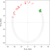Fig. 3 Possible paths of Venus’s spin pole in the BRF over 12 000 years, showing less than one period of the Chandler wobble. The motion corresponds to Eq. (40) for a liquid outer core. The thirty green dots show possible initial positions of the pole at epoch J2000. The red dots show the positions after 12 000 years, their spread reflecting the Chandler period range from Eq. (42). Fluctuations due to high-frequency forcing are too small to be seen at this scale (see Fig. 5).

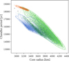Fig. 4 Chandler period of Venus computed for different interior models using Eq. (41). Colored bars correspond to the density profiles from Shah et al. (2022), featuring either a fully liquid core (green), a solid inner core with a liquid outer core (blue), or a fully solid core (orange). For each core state, the 99% contour of a kernel density estimate is shown. Black bars correspond to the density profiles from Dumoulin et al. (2017), all featuring fully liquid cores. The y-axis uncertainties are due to the lengthening of the Chandler period by tidal deformation (from 0.6% to 1.3% lengthening).

3.1.1 Period of the Chandler wobble

For the wobble frequency, due to the centrifugal and tidal bulges reacting to the wobble, we find an expression that is slightly modified from the rigid case Eq. (22): $$\begin{gathered} {\sigma }_{\mathrm{c}\mathrm{w}}=Re[{\alpha }_{\mathrm{c}\mathrm{w}}], \\ {\sigma }_{\mathrm{c}\mathrm{w}}=\mathrm{\Omega }s\sqrt{\frac{C-A-sRe[D]}{A+sRe[D]}\frac{C-B-sRe[D]}{B+sRe[D]}}, \end{gathered}$$(41)

where Re[D] = |D| cos δ_cw. Again, here, (A, B, C) are either the whole planet’s moments of inertia (core, mantle and atmosphere) or those without the core, depending on the core-mantle coupling assumption (see Sect. 4.2). With our current knowledge of the interior of Venus, the expected Chandler period is not well constrained: Figure 4 shows the possible values we obtain for a wide range of interior models.

In the case of Venus, the effect of mantle deformation D is small. Using the tidal responses from Musseau et al. (2024) with our Eq. (41), we find that the wobble period is slightly increased (compared to the rigid case Eq. (22)), with increases ranging from 0.6% for more viscous models to 1.3% for less viscous models. As noted by Van Hoolst (2015), this effect is minor because the mean shape of Venus is already far from hydrostatic equilibrium, so the tidal and rotational deformations have relatively little effect on the deviation from equilibrium: $s|D|\cos {\delta }_{\mathrm{c}\mathrm{w}}\ll C-A$.

As a result, the values obtained from Eq. (41) and from the rigid case Eq. (22) differ by less than 1.5%. Instead, the main source of uncertainty in determining the Chandler period resides in the value of the moment of inertia. If the outer core is liquid (green or blue in Fig. 4), only the mantle wobbles. Using the mantle moments of inertia from the density profiles of Shah et al. (2022), we find Cm/(M_vR²) ε [0.226; 0.328] when excluding profiles with a fully solid core. This gives a Chandler period range of $$P_{\mathrm{c}\mathrm{w}}=(2\pi /{\sigma }_{\mathrm{c}\mathrm{w}})\in [12900;18800]\text{\hspace{0.17em}years.}$$(42)

Otherwise in the case of a fully crystallized core (orange in Fig. 4), the planet wobbles as a whole. Using the moments of inertia from the density profiles of Shah et al. (2022), we find C/(MVR²) ε [0.317; 0.329] for these solid core cases, yielding a Chandler period in the range P_cw ε [18 100; 18 900] years. The ranges for the coupled (fully crystallized core) and decoupled (liquid outer core) cases overlap noticeably, so a measurement of polar motion alone may not be sufficient to distinguish between the two scenarios. This is discussed further in Sect. 4.4.

3.1.2 Damping of the Chandler wobble

From Eq. (38), we derive the characteristic damping time of the wobble. We identify two distinct damping processes, involving the tidal phase lags of both the pole tide and the semi-diurnal tide (58 days), respectively δ_cw and δ₃: $${\displaystyle \frac{1}{{\tau }_{\mathrm{c}\mathrm{w}}}}=\mathrm{I}\mathrm{m}[{\alpha }_{\mathrm{c}\mathrm{w}}]={\displaystyle \frac{1}{{\tau }^{(\mathrm{c}\mathrm{w})}}}+{\displaystyle \frac{1}{{\tau }^{(3)}}},$$(43)

with $${\tau }^{(\mathrm{c}\mathrm{w})}=\frac{1}{\mathrm{\Omega }{s}^2}\frac{fC}{\mathrm{I}\mathrm{m}[-\mathrm{D}]}=\frac{1}{\mathrm{\Omega }{s}^2}\frac{3G{M}_V}{{\mathrm{\Omega }}^2{R}^3}\frac{fC}{M_V{R}^2}{\displaystyle \frac{1}{-\mathrm{I}\mathrm{m}[{\mathrm{k}}_2^{(\mathrm{c}\mathrm{w}])}}},$$(44) $${\tau }^{(3)}=\frac{1}{\mathrm{\Omega }s}\frac{f^{\prime }C}{\mathrm{I}\mathrm{m}[-{\mathrm{D}}^{\prime }]}=\frac{1}{\mathrm{\Omega }(s-1)}\frac{G{M}_V}{n^2{R}^3}\frac{f^{\prime }C}{M_V{R}^2}\frac{1}{\mathrm{I}\mathrm{m}[{\mathrm{k}}_2^{(3)}]}$$(45)

with M_V and R the mass and radius of Venus, and f = AB/C² and $f^{\prime }=\frac{AB/C}{(A+B)/2}$ account for the non-sphericity of the planet, and are close to 1. With an interest only in the order of magnitude for the damping, these factors can be assumed equal to 1.

From our phase lag formalism, δ_cw and Ω have opposite signs, which results in τ^(cw) always being positive. Equation (44) agrees with the expression obtained by Yoder (1997). The effect of the solar torque appears in τ^(cw) through the factor s², which is around 7.6 for Venus, accounting for almost an order of magnitude faster damping. The tidal dissipation term Im[$k_2^{(\mathrm{c}\mathrm{w})}$], which should be taken at the period of the Chandler wobble of 16 000 years, is the least constrained factor in Eq. (44): the inelastic response of Venus has yet to be measured, and its elastic response is known only at the semi-diurnal period of 58 days. Venus’s tidal response can be extrapolated to low frequencies with a range of rheological models (Y. Musseau, priv. comm. 2024), obtaining values spanning nearly two orders of magnitude: $\mathrm{I}\mathrm{m}[{\mathrm{k}}_2^{(\mathrm{c}\mathrm{w})}]\in [0.003;0.2]$. Including uncertainties in the moment of inertia, we obtain τ^(cw) ε [0.8; 80] × 10⁶ years.

Interestingly, for Venus, the least viscous models result in less effective damping (up to 80 Myrs), while the most viscous models lead to more effective damping (down to 0.8 Myr). This can be explained by the fact that, at the Chandler period of around 16 000 years, for the tidal responses used here, the mantle’s behavior begins to approach its fluid limit, where the phase lag δ_cw tends toward zero. In this regime, a higher mantle viscosity moves the behavior further from the fluid limit, thereby increasing the phase lag and allowing for a more effective dissipation of the Chandler wobble. For most viscosity profiles, the phase lag of the pole tide is the dominant damping mechanism for Venus, with τ^(cw) < τ⁽³⁾.

The opposite is true only for the lowest-viscosity endmembers where Venus’s mantle viscosity is constant at 10¹⁹ Pas, and the phase lag of the semi-diurnal tide becomes the dominant damping mechanism. This additional damping Eq (45) has little effect for fast rotating planets, for which s is close to 1. The tidal dissipation term Im[$k_2^{(3)}$], evaluated at the semi-diurnal period of 58 days, varies by nearly an order of magnitude across the viscosity profiles considered: $-\mathrm{I}\mathrm{m}[{\mathrm{k}}_2^{(3)}]\in [0.002;0.02]$, leading to τ⁽³⁾ ε [9.7; 120] × 10⁶ years. Combining both contributions in Eq (43), with the tidal responses used here (Musseau, priv. commun.), we find an overall Chandler wobble damping time within: $${\tau }_{\mathrm{c}\mathrm{w}}\in [0.8;13]\times {10}^6\text{\hspace{0.17em}years.}$$(46)

The damping is barely too slow to be noticeable in Fig. 3, which covers only 12 000 years. It is fast enough however, that an excitation process near the Chandler frequency is required to explain the measured angle 0.481° ± 0.020° (Konopliv et al. 1999) between the spin axis and the figure axis.

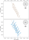Fig. 5 Path of Venus’s spin pole in the BRF over 4 years (2034-2038). The gray line represents the free wobble, appearing as a linear trend at this scale. Colored curves show the polar motion caused by: the solar torque only (top panel), the solar torque and the atmosphere (bottom panel, light blue), the solar torque and just the 117-day atmospheric contribution (bottom panel, dark blue, added for readability). Initial positions are indicated with dots. For reference, the surface resolution of EnVision’s VenSAR is indicated, for the regional (30 m) and targeted (10m) imaging.

3.2 High-frequency forced polar motion

The polar motion forced response m_F from Eq. (36) is $$\begin{gathered} m_F(t)=\sum _k{F}_k{e}^{i{\nu }_{k}t}\frac{\mathrm{\Omega }s(C^{\prime }-\frac{A^{\prime }+B^{\prime }}{2})+{\nu }_k\frac{A^{\prime }+B^{\prime }}{2}}{i{A}^{\prime }{B}^{\prime }({\nu }_k^2-{\alpha }_{\mathrm{c}\mathrm{w}}^2)} \\ +\sum _k\overline{F}{e}^{-i{\nu }_{k}t}\frac{(\mathrm{\Omega }s-{\nu }_k)\frac{B^{\prime }-A^{\prime }}{2}}{i{A}^{\prime }{B}^{\prime }({\nu }_k^2-{\alpha }_{\mathrm{c}\mathrm{w}}^2)}, \end{gathered}$$(47)

where A′ =A+sD, B′ =B+sD and C′ = C-D′. Here the complex value of α_cw again encompasses a damping behavior, preventing an infinite response at $|{\nu }_k|=|{\alpha }_{\mathrm{c}\mathrm{w}}|$.

The excitation terms found in the solar torque Eqs. (18), (28), and (29) and in the tidal deformation Eq. (26), along with the atmospheric excitation Eq. (33), all have periods of a few hundred days maximum. The excitation we consider here is thus in the high-frequency regime when compared to the resonant frequency, with |v_k| >> |α_cw| ≈ 2π/16 000 yr. In this regime, considering (C - A) ≪ A and (B - A) ≪ A, the transfer function in Eq. (47) acts as a simple low-pass filter in 1/ν: $$m_F(t)=-i\frac{A^{\prime }+B^{\prime }}{2A^{\prime }{B}^{\prime }}\sum _k\frac{1}{{\nu }_k}{F}_k{e}^{i{\nu }_{k}t},$$(48) $$m_F(t)\approx -\frac{i}{C}\sum _k\frac{1}{{\nu }_k}{F}_k{e}^{i{\nu }_{k}t}.$$(49)

In particular, within m_F, the response m_A to the atmospheric excitation terms from Eq. (33) can be written as $$m_A(t)=-\frac{1}{C}\sum _k(\frac{1}{\mathrm{\Omega }}+\frac{1}{{\nu }_k})(\mathrm{\Delta }{h}_k+\mathrm{\Omega }\mathrm{\Delta }{I}_k)e^{i{\nu }_{k}t},$$(50)

where for higher frequencies |v_k| >> |Ω| = 2π/243d, the transfer function becomes constant at -(CΩ)⁻¹. This is convenient when needing to input the raw signal given by the V-PCM, with any high-frequency noise in Δh_a simply multiplied by this constant.

The transfer function Eq. (50) cancels out for ν = -Ω, which happens the be the dominant component of Δh_a (Table 2). As a consequence, in Fig. 2, the 243-day periodicity in Δh_a (blue) is filtered-out in ma (orange) by the transfer function, leaving the +117 days and −117 days contributions as the dominant components in the atmosphere-induced polar motion. The high-frequency noise is passed unchanged from Δh_a to m_a, where it appears at the same scale for both in Fig. 2 due to the choice of normalization.

Given the finite 2333-day span of the atmospheric simulation, small-amplitude components with periods of ±2333 days and ±1167 days appear in Δh_a, both in the Discrete Fourier Transform and the frequency decomposition. The frequency analysis for such low frequencies is unreliable, and these components could result from a trend or from longer periods generated by the Venus Planetary Climate Model. For this reason, we manually filter out periods longer than 800 days in Δh_a, as these require longer time series in order to be properly analyzed. If such low frequency truly exist in Δh_a, they would be significantly amplified in the polar motion through the transfer function Eq. (47).

Applying the transfer function Eq. (49) to each excitation term, we find that the major contributors to the forced polar motion of Venus are the atmospheric winds and the solar torque, as detailed in Table 4. Figure 5 depicts the polar motion of Venus without and with the atmospheric contribution. When measuring the Chandler frequency, the signal of interest is the average speed of the spin pole along its linear trend (gray line), while the forced fluctuations are regarded as additional noise. The potential detection and measurement of the polar motion by future Venus orbiters is discussed in Sect. 4.4.

Mantle internal dynamics, core-mantle interactions, and low-frequency atmospheric dynamics could also contribute to the excitation of Venus’s polar motion through variations in the mantle’s angular momentum and mass distribution. A long-period excitation process is required to explain the current amplitude of its polar motion. It could be a geologically recent event, in which case the observed amplitude would correspond to a purely decaying Chandler wobble, or it could be an ongoing process that actively sustains a large amplitude. Low-frequency excitation is beyond the scope of this work, and further study is needed to determine whether its effects are significant enough to be detected in future measurements.

4 Discussion

4.1 Influence of atmosphere super-rotation

The wind-induced excess angular momentum, h, is calculated for Venus using the V-PCM with Eq. (30). It has a non-zero average, indicating that the atmosphere is in a state of global super-rotation. We find that this average component is close to the spin axis, with an offset of only 127 arcseconds, which led us to assume in Eq. (5) that it is aligned with the spin axis. This is a first approach, and a more detailed model of the super-rotation axis orientation could be explored in future work.

Here we focus on the effects of super-rotation on polar motion by deriving again Eq. (6) while keeping the terms from the mean super-rotation excess angular momentum, h_sr. We normalize the coefficient k by the mean polar moment of inertia of the atmosphere, I_a, introducing a dimensionless super-rotation coefficient S identical to that of Mendonça & Read (2016): $$h_{sr}=S{I}_a\omega .$$(51)

Defined this way, S represents the ratio of the wind-induced angular momentum to the angular momentum of a windless atmosphere. In the absence of super-rotation, S = 0. Using the V-PCM, with the third component of Eqs. (30) and (31) we compute the mean values $\Vert h_{sr}\Vert =2.0\times {10}^{28}\mathrm{k}\mathrm{g}{\mathrm{m}}^2{\mathrm{s}}^{-1}$ = 2.0 × 10²⁸ kg m² s⁻¹ and Ia = 1.2 × 10³⁴ kg m². This corresponds to a global superrotation coefficient S = 5.7, which is consistent with the value $S={7.66}_{-3.6}^{+4.2}$ estimated by Mendonça & Read (2016) based on available observational data.

Equation (6) becomes $$\begin{gathered} (A+S{I}_a)\dot{m_x}+\dot{\mathrm{\Delta }{\mathcal{I}}_{xz}}+\frac{1}{\mathrm{\Omega }}\dot{\mathrm{\Delta }{h}_x}+\mathrm{\Omega }(C-B)m_y-\mathrm{\Omega }\mathrm{\Delta }{\mathcal{I}}_{yz}-\mathrm{\Delta }{h}_y=\frac{1}{\mathrm{\Omega }}{\mathrm{\Gamma }}_x \\ (B+S{I}_a)\dot{m_y}+\dot{\mathrm{\Delta }{\mathcal{I}}_{yz}}+\frac{1}{\mathrm{\Omega }}\dot{\mathrm{\Delta }{h}_y}-\mathrm{\Omega }(C-A)m_x+\mathrm{\Omega }\mathrm{\Delta }{\mathcal{I}}_{xz}+\mathrm{\Delta }{h}_x=\frac{1}{\mathrm{\Omega }}{\mathrm{\Gamma }}_y \\ (C+S{I}_a)\dot{m_z}+\dot{\mathrm{\Delta }{\mathcal{I}}_{zz}}+\frac{1}{\mathrm{\Omega }}\dot{\mathrm{\Delta }{h}_z}=\frac{1}{\mathrm{\Omega }}{\mathrm{\Gamma }}_z. \end{gathered}$$(52)

Here, we notice that the super-rotation adds k = SI_α to the moments of inertia (A, B, C), essentially increasing the effective inertia of the planet. The Chandler frequency becomes $${\sigma }_{\mathrm{c}\mathrm{w}}=\mathrm{\Omega }s\sqrt{\frac{C-A-sRe[D]}{A+sRe[D]+S{I}_a}\frac{C-B-sRe[D]}{B+sRe[D]+S{I}_a}},$$(53)

where the super-rotation slightly increases the Chandler period. We find the effect to be negligible for Venus: it slows down the wobble by a factor of about S I_a/C_m, with the super-rotation coefficient S = 5.7 and the atmosphere/mantle inertia ratio of I_a/C_m = 1/4000, for a overall period increase of only 0.1%.

4.2 Influence of core-mantle coupling

At the core-mantle boundary, a viscosity discontinuity may lead to dynamical decoupling, where the core and the mantle rotate at different speeds and around different axes, exerting a viscous torque on each other. Depending on the core’s effective viscosity at the boundary, the Chandler wobble of the mantle may or may not translate to the core. This makes the Chandler period particularly sensitive to the physical state of the core.

Previously, we only considered the two limiting cases in which the core of Venus is either decoupled from the mantle (zero torque) or fully locked with it (infinite torque). Here, in this section, we analyze a toy model with a finite coupling coefficient showing that our results in Sect. 3 hold in both limiting cases, provided that the moments of inertia used in the equations are those of the mantle only in the decoupled case, instead of those of the whole planet that are used in the locked case.

Our simplified model in this section is a planet with a rigid axisymmetric mantle and a spherical core whose moment of inertia is I_c. The rotation vectors of the mantle and the core, ω and ω_c, can differ, resulting in a torque at the core-mantle boundary. A spherical interface implies that the torque exerted on the mantle by the core lies in the direction of the differential rotation (Aoki 1969): $${\mathrm{\Gamma }}_c=k_c({\omega }_c-\omega ),\text{with k\_c > 0,}$$(54)

where k_c is the coupling coefficient. As in Sect. 2.2, we also take into account the solar torque exerted on the mantle.

Similarly to Eq. (2), the core’s spin axis remains close to the z-axis and we write it as ${\omega }_c=\mathrm{\Omega }(m_{c,x},m_{c,y},1+m_{c,z}{)}^T$ where m_c,x, m_c,y, and m_c,z are treated as small quantities. We consider two Euler rotation equations, one for the mantle and one for the whole planet, which become $$\begin{gathered} A_m\dot{m}-i\mathrm{\Omega }s(C-A)m=k_c(m_c-m) \\ {A}_m\dot{m}-i\mathrm{\Omega }s(C-A)m+I_c\dot{m_c}+i\mathrm{\Omega }{I}_c(m_c-m)=0, \end{gathered}$$(55)

where A_m = A - I_c is the smallest moment of inertia of the mantle. Here, the factor s = 1 + (3n²)/(2Ω²) comes directly from the solar torque Eq. (18), computed for an axisymmetric mantle. With this system of equations, we find a damped wobble for m, whose period and characteristic damping time are $${\sigma }_c=\mathrm{\Omega }s(C-A)\frac{KA+\frac{1}{K}{A}_m}{K{A}^2+\frac{1}{K}{A}_m^2},$$(56) $${\tau }_c=\frac{1}{\mathrm{\Omega }s}\frac{K{A}^2+\frac{1}{K}{A}_m^2}{(C-A)I_c},$$(57)

where K = k_c/(I_c Ω) is the normalized coupling coefficient. We note that, while K and σ_c have the same sign as ω, the damping time, τ_c, remains positive.

As expected for the wobble period, in the locked case with |K| >> 1, we find σ_c = Ωs(C - A)/A as for a fully rigid body. In the decoupled case with |K ≪ 1, where only the mantle’s inertia opposes the wobble, we find a faster wobble σ_c = Ωs(C - A)/A_m. Between both regimes, there is a continuous transition at values of |K| around (A_m/A)² ≈ 1, as shown in Fig. 6.

It is currently uncertain whether Venus’s core is entirely solid, entirely liquid, or consists of a liquid outer core with a solid inner core (Dumoulin et al. 2017). If the entire core has crystallized, then $|K|\to \mathrm{\infty }$ and Venus wobbles as a single unit. In that case, the Chandler period would serve as a proxy for the total inertia of the planet, similarly to the precession period. On the other hand, if the core has an outer liquid layer or is fully liquid, the coupling coefficient |K| is very weakly constrained. The ranges of kinematic viscosities considered for Venus by both Yoder (1997) and Correia et al. (2003) indicate that a turbulent friction regime is expected, where |K| ≪ 1, which implies that a liquid outer core would not wobble along with the mantle. In that case, the Chandler period serves as a proxy for the mantle’s inertia.

The wobble damping caused by core-mantle friction is most efficient for values of |K| around (A_m /A)² ≈ 1, where it can become the dominant damping process, with the coremantle damping time τ_c falling below the [10⁶; 10⁷] years range obtained for the mantle deformation damping time τ_cw in Sect. 3.1.2. In the coupled and decoupled limiting cases, however, there is no core-mantle damping occurring, and the dominant process remains mantle deformation damping.

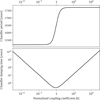Fig. 6 Period and damping time of the Chandler wobble for a simplified Venus (rigid axisymmetric mantle and spherical core), as a function of the core-mantle coupling coefficient.

4.3 Comparison with Earth and Mars

Among the planets, the Chandler wobble has been detected on Earth (Chandler 1891) and Mars (Konopliv et al. 2020). Both planets rotate more than two orders of magnitude faster than Venus and are thus much more oblate, with their (C - A)/A also being more than two orders of magnitude larger than that of Venus. As a result, the expected wobble for Venus is four orders of magnitude slower than the Chandler wobble measured on Earth or Mars (see Table 5). In this slow spin regime, the interior properties that influence a planet’s Chandler period differ from those in a fast rotation regime.

The solar torque causes a faster wobble, but this effect is significant only for slowly rotating planets (see Sect. 2.2). For Earth and Mars, where Ω² >> n², the wobble frequency increases by less than 0.001%, well below current measurement accuracy. In contrast, for Venus, |Ω| = 0.92n, resulting in a wobble frequency increase by a factor of 2.75.

Solid mantle deformations slow down the wobble, lengthening its period by a factor of approximately |1 - sD/(C - A)| (see Sect. 2.3). This effect is more pronounced for fast-rotating planets, where the factor is expressed as $|1-k_2^{(\mathrm{c}\mathrm{w})}/k_2^{(f)}|$, as their oblateness factor C - A is primarily due to the hydrostatic rotational bulge. Here, $k_2^{(f)}$ is the Love number in the fluid limit, at the frequency 0. This leads to a 38% increase in Earth’s Chandler period and a 16% increase for Mars, when comparing the measured values (Table 5) to those obtained using Eq. (22). For Venus, which rotates more slowly, the non-hydrostatic contribution to C - A becomes dominant, resulting in |sD/(C - A)| 1 and reducing the impact of solid deformation. Comparing the values obtained with Eqs. (22) and (41), we find that this effect increases the Chandler period by less than 1.5%.

The amplitude of the Chandler wobble, unlike its period, cannot be solely linked to the planet’s internal structure, as it depends on the excitation mechanisms near the Chandler frequency. With an estimate of the damping efficiency of the wobble (see Sect. 3.1.2), measuring the amplitude could help characterize these excitation sources as they sustain the wobble. On Earth, the amplitudes of both free motion (Chandler wobble) and forced motion are comparable, around 150 milliarcseconds (Gross 2000). On Mars, the free motion amplitude is 6 milliarcseconds, about four times weaker than the forced motion (Konopliv et al. 2020). In contrast, Venus’s predicted wobble amplitude of 0.5° is four orders of magnitude larger than Earth’s. That is three orders of magnitude larger than the forced motion expected from atmospheric dynamics and solar torque.

The combined excitation from Earth’s ocean and atmosphere near its Chandler period of 433 days has been shown sufficient to sustain its observed wobble (Gross 2015), essentially through their inertia terms, noted ΔI_a in our work. For Mars, Dehant et al. (2006) identify atmospheric stochastic excitation as the primary excitation source of the wobble at 207 days. For Venus, the source of wobble excitation is still an open question.

As a result of the contrasts in the Chandler wobble’s periods and amplitudes, the detection methods vary between planets. For the first detection of Earth’s Chandler wobble, Chandler (1891) relied on ground-based stellar observations spanning nearly a full period. For Mars, the wobble was detected through its effect on Mars orbiters trajectories, using spacecraft tracking data spanning 21 years thus covering tens of periods (Konopliv et al. 2020). For Venus, with an expected Chandler period of around 16 000 years, even a similar 20-year observational coverage would represent only 0.1% of a full period. At this timescale, the wobble manifests as a linear trend rather than a periodic signal (see Fig. 5). However, the large amplitude - 52 km when projected onto Venus’s surface - could still make polar motion detectable by future orbiters, despite its long period.

4.4 Observations with EnVision

ESA’s EnVision and NASA’s VERITAS, two spacecraft currently scheduled for launch no earlier than 2031, are set to study Venus from low, circular, polar orbits, with a focus on geophysics as part of their missions (Widemann et al. 2023). We focus on EnVision, one of its objectives being to “determine the size of the major internal layers (. . . ) and the state of the core, to better understand Venus’ thermo-chemical evolution” (ESA 2023). This will be achieved by its radio science and radar experiments, which will measure Venus’s gravity field and rotational dynamics.

The synthetic aperture radar, VenSAR, in its imaging mode, will provide repeated views of regions of interest on Venus’s surface. This will enable the construction of a geodetic control network by matching radar features across multiple images and solving for their surface coordinates along with a planetary rotation model. For Venus, this approach was first implemented by Davies et al. (1992) using Magellan radar images, recovering its rotation period and spin axis orientation, though without sufficient resolution to detect the precession or polar motion signals.

The Radio Science Experiment (RSE), in its gravity experiment mode, will produce Doppler tracking data of the EnVision spacecraft, enabling the joint recovery of Venus’s gravitational field and spacecraft trajectory. If the gravity field is considered attached to a body-fixed reference frame, a rotation model can be derived simultaneously. Alternatively, if the gravity field is considered attached to the spin reference frame (SRF, see Fig. 1), the polar motion signal is seen instead as variations in the degree-2 gravity coefficients C₂₁ and S₂₁. For Mars, both approaches were implemented by Konopliv et al. (2020), yielding consistent results. For Venus, Magellan tracking data provided a gravity field solution (Konopliv et al. 1999), albeit only using the predetermined, uniform rotation model of Davies et al. (1992). Recovering Venus’s spin axis precession from Doppler tracking data has already been proposed and simulated for the next Venus missions (Rosenblatt et al. 2021; Cascioli et al. 2021), but the recovery of its polar motion has not been similarly studied.

The combined capabilities of VenSAR and RSE could enable a joint inversion of the gravitational field, spacecraft trajectory, control network, and rotation model. Cascioli et al. (2021) propose this approach for the future VERITAS mission, simulating its VISAR radar and Doppler tracking system, with a rotation model that includes the spin orientation and precession, without the polar motion. They find that the synergy between tie points and Doppler observations should allow for the detection of Venus’s precession, with a 0.3% relative uncertainty for its period.

The polar motion model developed here suggests that, over EnVision’s 4-year primary mission, Venus’s polar motion could be detected alongside its precession. During this period, the spin axis precesses by 8 arcseconds in inertial space, a motion corresponding to 240 meters at the surface, while the Chandler wobble appears as a drift of approximately 90 meters of the spin pole in a body-fixed reference frame. This implies that a surface feature initially coincident with the spin axis, would, after four years, trace circular paths with a radius of 90 meters in inertial space, with a period of 243 days. Such motion should be accounted for: not only to measure the Chandler period, but also to potentially strengthen the determination of the precession period. Additionally, the signal of polar motion could be enhanced by combining future radar and Doppler data from both EnVision and VERITAS. Both Earth-based and Magellan’s radar observations have lower resolution, but the long time span between their datasets and those of future missions might still make them valuable for detecting Venus’s polar motion.

The science operations of EnVision are currently planned to begin in 2034 and could measure both the precession and wobble periods. Figure 7 shows both of these observables for the wide range of interior models produced by Shah et al. (2022). If both periods yield compatible values for Venus’s total moment of inertia, it indicates that both motions are opposed by the same total inertia (orange dotted line). It would imply that the core is locked to the mantle even for the Chandler wobble motion, leading to the conclusion that the core is fully solid (see Sect. 4.2). However, if the two estimates of moments of inertia obtained are incompatible, it would indicate that the core is not fully solid (blue and green regions in Fig. 7), in which case the moment of inertia derived from the wobble corresponds to the mantle alone. Based on interior modeling (e.g., Shah et al. 2022), measuring both periods would provide a refined estimate of Venus’s core size: interior models which have the same total moment of inertia and the same mantle moment of inertia also have similar core sizes, to within 50 km, allowing core size level lines to be drawn in Fig. 7.

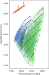Fig. 7 Chandler and precession periods of Venus computed for the density profiles of Shah et al. (2022), featuring either a fully liquid core (green), a solid inner core with a liquid outer core (blue), or a fully solid core (orange). For each core state, the 99% contour of a kernel density estimate is shown. Black bars correspond to the density profiles from Dumoulin et al. (2017), all featuring fully liquid cores. Black level lines indicate the core size of the models in kilometers, to within 50 km.

5 Conclusions

This work provides a comprehensive model of Venus’s polar motion. Incorporating the effects of solar torque, mantle viscoelasticity, and atmospheric dynamics, we derived the Chandler wobble period and damping time, as well as the frequencies and amplitudes of the forced motion, with expressions that are valid for both slowly and rapidly rotating terrestrial planets.

To apply this model to Venus, we used available measurements (Konopliv et al. 1999; Margot et al. 2021) and relied on interior models (Shah et al. 2022; Musseau et al. 2024). Our results emphasize the significant role of the solar torque in accelerating the Chandler wobble with a factor of 2.75, predicting a wobble period ranging between 12 900 and 18 900 years, depending on the state of Venus’s core and the moments of inertia of the mantle and of the whole body. This wobble is damped on timescales ranging from 0.8 to 13 million years, with poor constraints for Venus’s dissipation efficiency at these low frequencies.

We addressed the high-frequency excitation of Venus’s polar motion by atmospheric dynamics and solar torque, which operate at periods up to a few hundred days, predicting the high-frequency polar motion to be accounted for when searching for the free Chandler wobble signal. However, the long-period excitation required to explain the current amplitude should be explored further to determine whether it could contribute to the polar motion measured by future missions.

We highlight the necessity of incorporating polar motion into Venus rotation models when anticipating the upcoming orbiter missions. Over EnVision’s 4-year mission, the predicted ~90-meter polar shift in body-fixed frame due to the Chandler wobble, along with the ~240-meter shift in inertial space due to precession, should be measurable. If both motions are indeed detected by the EnVision mission, the physical state of the core would be determined. If Venus’s core is not found to be fully solid, the Chandler period is a proxy for the mantle’s moment of inertia, providing refined constraints for the size of the core and for thermo-chemical properties of Venus’s interior.

Acknowledgements

We thank R. Helled and O. Shah for providing the Venus density profiles, S. Lebonnois and E. Millour for providing atmospheric simulation data with assistance in reading it, and Y. Musseau for contributing tidal response curves. We thank R.-M. Baland for the careful review.

Appendix A Numerical parameters used for Venus

Appendix B Derivation of the torque acting on the tidal bulges

Here we use the notation {X} to denote the tidal response of Venus to a perturbation X: $$X(t)=\widetilde{k_2}(\tau )\ast X(t)={\int }_0^{+\mathrm{\infty }}\widetilde{k_2}(\tau )X(t-\tau )d\tau ,$$(B.1)

where $\widetilde{k_2}(\tau )$ is the convolution kernel that encompasses the body’s rheological properties. With this notation, perturbations with opposite frequencies are associated with conjugate love numbers (e.g., Efroimsky 2012): if $e^{i{\nu }_{j}t}=k_2^{(j)}{e}^{i{\nu }_{j}t}$ then $e^{-i{\nu }_{j}t}=\overline{k_2^{(j)}}{e}^{-i{\nu }_{j}t}$. With conjugate love numbers having opposite phase lags, then all time lags remain negative, as physically expected.

For clarity, the tidal deformation is first expressed with the notation {.}, and we switch to using the individual $k_2^{(j)}$ values from Table 1 when the frequencies are separately identified.

B.1 Solar torque on the centrifugal bulge

Using the coordinates r of the Sun in the BRF (Eq. 15), we derive the solar torque Γ_R acting on Venus’s centrifugal deformation: $${\mathrm{\Gamma }}_R=3\frac{G{M}_{\odot }}{\Vert r{\Vert }^5}r\times \mathrm{\Delta }{\mathcal{I}}_{R}r,\text{with}\mathrm{\Delta }{\mathcal{I}}_R=\frac{{\mathrm{\Omega }}^2{R}^5}{3G}\left[\begin{array}{c}-\frac{2}{3}{m}_{z}0m_x\\ 0-\frac{2}{3}{m}_z{m}_y\\ m_x{m}_y\frac{4}{3}{m}_z\end{array}\right],\text{and}\frac{r}{\Vert r\Vert }=\left[\begin{array}{c}x\\ y\\ z\end{array}\right],$$(B.2) $${\mathrm{\Gamma }}_R=\frac{n^2{\mathrm{\Omega }}^2{R}^5}{G}\left[\begin{array}{c}xy{m}_x+y^2{m}_y\\ -x^2{m}_x-xy{m}_y\\ 0\end{array}\right],$$(B.3)

where we considered only the first-order terms in ε and β. With T_R = Γ_R,x + iΓ_R,y, we have $$T_R=\frac{n^2{\mathrm{\Omega }}^2{R}^5}{2G}[(y^2+x^2)m_y-i{m}_x+(y^2-x^2-2ixy)m_y+i{m}_x],$$(B.4) $$T_R=\frac{n^2{\mathrm{\Omega }}^2{R}^5}{2G}[\beta e^{-i\alpha }-e^{i({\theta }_3-\alpha )}\beta e^{i\alpha }].$$(B.5)

We then finally obtain $$T_R=-i{k}_2^{(\mathrm{c}\mathrm{w})}\frac{n^2{\mathrm{\Omega }}^2{R}^5}{2G}m-\overline{k_2^{(\mathrm{c}\mathrm{w})}}\beta \frac{n^2{\mathrm{\Omega }}^2{R}^5}{2G}{e}^{i{\theta }_3}.$$(B.6)

B.2 Solar torque on the solar tidal bulge

We then derive the solar torque Γ_T acting the solar tidal deformation: $${\mathrm{\Gamma }}_T=3\frac{G{M}_{\odot }}{\Vert r{\Vert }^5}r\times \mathrm{\Delta }{\mathcal{I}}_{T}r,\text{with}\mathrm{\Delta }{\mathcal{I}}_T=-\frac{n^2{R}^5}{G}\left[\begin{array}{c}{x}^2-\frac{1}{2}xyxz\\ xy{y}^2-\frac{1}{2}yz\\ xzyz0\end{array}\right],\text{and}\frac{r}{\Vert r\Vert }=\left[\begin{array}{c}x\\ y\\ z\end{array}\right].$$(B.7) $${\mathrm{\Gamma }}_T=-3\frac{n^4{R}^5}{G}\left[\begin{array}{c}xyxz+y^{2}yz-xzxy-yz{y}^2-\frac{1}{2}\\ xz{x}^2-\frac{1}{2}+yzxy-x^{2}xz-xyyz\\ x^{2}xy+xy{y}^2-\frac{1}{2}-xy{x}^2-\frac{1}{2}-y^{2}xy\end{array}\right],$$(B.8)

where we considered only the first-order terms in ε and β. With $T_R={\mathrm{\Gamma }}_{R,x}+i{\mathrm{\Gamma }}_{R,y}$, we have $$T_T=-\frac{3}{2}\frac{n^4{R}^5}{G}[(y^2+x^2)yz-ixz-(x^2-y^2+2ixy)yz+ixz+(yz+ixz)x^2-y^2+2ixy-(yz-ixz)y^2+x^2-1],$$(B.9) $$\begin{gathered} T_T=-\frac{3}{4}\frac{n^4{R}^5}{G}[-ϵe^{i{\theta }_1}+ϵe^{i{\theta }_2}+\beta e^{i{\theta }_3}-\beta e^{-i\alpha } \\ -e^{i({\theta }_3-\alpha )}-ϵe^{-i{\theta }_1}+ϵe^{-i{\theta }_2}+\beta e^{-i{\theta }_3}-\beta e^{i\alpha }+(-ϵe^{-i{\theta }_1}+ϵe^{-i{\theta }_2}+\beta e^{-i{\theta }_3}-\beta e^{i\alpha })e^{i({\theta }_3-\alpha )}]. \end{gathered}$$(B.10)

Noticing that θ₁ + θ₂ = θ₃ - α, $$\begin{gathered} T_T=-\frac{3}{4}\frac{n^4{R}^5}{G}[(-k_2^{(1)}ϵe^{i{\theta }_1}+k_2^{(2)}ϵe^{i{\theta }_2}+k_2^{(3)}\beta e^{i{\theta }_3}-k_2^{(\mathrm{c}\mathrm{w})}\beta e^{-i\alpha }) \\ -(-\overline{k_2^{(1)}}ϵe^{i{\theta }_2}+\overline{k_2^{(2)}}ϵe^{i{\theta }_1}+\overline{k_2^{(3)}}\beta e^{-i\alpha }-\overline{k_2^{(\mathrm{c}\mathrm{w})}}\beta e^{i{\theta }_3})+(-k_2^{(3)}ϵe^{i{\theta }_2}+k_2^{(3)}ϵe^{i{\theta }_1}+k_2^{(3)}\beta e^{-i\alpha }-k_2^{(3)}\beta e^{i{\theta }_3})]. \end{gathered}$$(B.11)

We then finally obtain $$T_T=-i\frac{3}{4}\frac{n^4{R}^5}{G}(k_2^{(\mathrm{c}\mathrm{w})}+\overline{k_2^{(3)}}-k_2^{(3)})m+\frac{3}{4}\frac{n^4{R}^5}{G}[(k_2^{(1)}+\overline{k_2^{(2)}}-k_2^{(3)})ϵe^{i{\theta }_1}-(\overline{k_2^{(1)}}+k_2^{(2)}-k_2^{(3)})ϵe^{i{\theta }_2}-\overline{k_2^{(\mathrm{c}\mathrm{w})}}\beta e^{i{\theta }_3}].$$(B.12)

References

- Aoki, S. 1969, AJ, 74, 284 [Google Scholar]
- Baland, R.-M., Coyette, A., & Van Hoolst, T. 2019, Celest. Mech. Dyn. Astron., 131 [CrossRef] [Google Scholar]
- Bizouard, C. 2020, Geophysical Modelling of the Polar Motion (De Gruyter) [CrossRef] [Google Scholar]
- Boué, G., Correia, A. C. M., & Laskar, J. 2016, Celest. Mech. Dyn. Astron., 126, 31 [CrossRef] [Google Scholar]
- Cascioli, G., Hensley, S., De Marchi, F., et al. 2021, Planet. Sci. J., 2, 220 [Google Scholar]
- Chandler, S. C. 1891, AJ, 11, 59 [NASA ADS] [CrossRef] [Google Scholar]
- Correia, A. C. M., & Valente, E. F. S. 2022, Celest. Mech. Dyn. Astron., 134 [CrossRef] [Google Scholar]
- Correia, A. C. M., Laskar, J., & Néron de Surgy, O. 2003, Icarus, 163, 1 [NASA ADS] [CrossRef] [Google Scholar]
- Cottereau, L., Rambaux, N., Lebonnois, S., & Souchay, J. 2011, A&A, 531, A45 [NASA ADS] [CrossRef] [EDP Sciences] [Google Scholar]
- Davies, M. E., Colvin, T. R., Rogers, P. G., et al. 1992, JGR Planets, 97, 13141 [Google Scholar]
- Dehant, V., de Viron, O., & Greff-Lefftz, M. 2005, A&A, 438, 1149 [NASA ADS] [CrossRef] [EDP Sciences] [Google Scholar]
- Dehant, V., de Viron, O., Karatekin, O., & Van Hoolst, T. 2006, A&A, 446, 345 [NASA ADS] [CrossRef] [EDP Sciences] [Google Scholar]
- Dumoulin, C., Tobie, G., Verhoeven, O., Rosenblatt, P., & Rambaux, N. 2017, JGR Planets, 122, 1338 [Google Scholar]
- Efroimsky, M. 2012, Celest. Mech. Dyn. Astron., 112, 283 [NASA ADS] [CrossRef] [Google Scholar]
- ESA 2023, EnVision - Understanding why Earth’s closest neighbour is so Different, Definition Study Report (Red Book), ESA document reference [Google Scholar]
- Gastineau, M., & Laskar, J. 2011, ACM Commun. Comput. Algebra, 44, 194 [Google Scholar]
- Gross, R. S. 2000, Geophys. Res. Lett., 27, 2329 [Google Scholar]
- Gross, R. S. 2015, in Treatise on Geophysics (Elsevier), 215 [Google Scholar]
- Konopliv, A. S., & Yoder, C. F. 1996, Geophys. Res. Lett., 23, 1857 [CrossRef] [Google Scholar]
- Konopliv, A. S., Banerdt, W. B., & Sjogren, W. L. 1999, Icarus, 139, 3 [Google Scholar]
- Konopliv, A. S., Park, R. S., Rivoldini, A., et al. 2020, Geophys. Res. Lett., 47 [CrossRef] [Google Scholar]
- Lai, D., Lebonnois, S., &Li, T. 2024, JGR Planets, 129, e2023JE008253 [Google Scholar]
- Laskar, J. 1993, Celest. Mech. Dyn. Astron., 56, 191 [NASA ADS] [CrossRef] [Google Scholar]
- Lebonnois, S., Hourdin, F., Eymet, V., et al. 2010, JGR Planets, 115, E06006 [Google Scholar]
- Margot, J.-L., Campbell, D. B., Giorgini, J. D., et al. 2021, Nat. Astron., 5, 676 [NASA ADS] [CrossRef] [Google Scholar]
- Mendonça, J. M., & Read, P. L. 2016, Planet. Space Sci., 134, 1 [CrossRef] [Google Scholar]
- Munk, W. H., & MacDonald, G. J. 1960, The Rotation of the Earth: A Geophysical Discussion (Cambridge University Press) [Google Scholar]
- Musseau, Y., Tobie, G., Dumoulin, C., et al. 2024, Icarus, 422, 116245 [Google Scholar]
- Rambaux, N. 2013, A&A, 556, A151 [NASA ADS] [CrossRef] [EDP Sciences] [Google Scholar]
- Rambaux, N., Castillo-Rogez, J., Dehant, V., & Kuchynka, P. 2011, A&A, 535, A43 [NASA ADS] [CrossRef] [EDP Sciences] [Google Scholar]
- Rosenblatt, P., Dumoulin, C., Marty, J.-C., & Genova, A. 2021, Remote Sensing, 13, 1624 [Google Scholar]
- Saliby, C., Fienga, A., Briaud, A., Mémin, A., & Herrera, C. 2023, Planet. Space Sci., 231, 105677 [CrossRef] [Google Scholar]
- Shah, O., Helled, R., Alibert, Y., & Mezger, K. 2022, ApJ, 926, 217 [Google Scholar]
- Spada, G., Sabadini, R., & Boschi, E. 1996, Geophys. Res. Lett., 23, 1997 [Google Scholar]
- Van Hoolst, T. 2015, in Treatise on Geophysics (Elsevier), 121 [Google Scholar]
- Widemann, T., Smrekar, S. E., Garvin, J. B., et al. 2023, Space Sci. Rev., 219, 56 [NASA ADS] [CrossRef] [Google Scholar]
- Williams, J. G. 1994, AJ, 108, 711 [Google Scholar]
- Williams, J. G., Boggs, D. H., Yoder, C. F., Ratcliff, J. T., & Dickey, J. O. 2001, JGR Planets, 106, 27933 [Google Scholar]
- Yoder, C. F. 1997, in Venus II (University of Arizona Press), 1087 [Google Scholar]
- Yoder, C. F., & Ward, W. R. 1979, ApJ, 233, L33 [Google Scholar]
All Tables
Composite angles involved in the forcing of Venus’s polar motion and associated Love numbers.
Periodic components of the atmospheric equatorial angular momentum computed with the V-PCM.
Periodic components of the atmospheric moment of inertia computed with the V-PCM.
Periodic components of Venus’s forced polar motion response projected on its surface: .