© The Authors 2024

1 Introduction

Tidal dissipation is one of the main mechanisms for energy loss in planetary systems. Since the seminal work in Darwin (1879), many scientists have investigated the effects of tidal forces in the dynamical evolution of celestial bodies, which modify orbital elements and spin orientations, and lead to diverse dynamical phenomena such as spin-orbit coupling and planetary migration (e.g. Goldreich & Peale 1966; Boué & Efroimsky 2019; Correia & Delisle 2019; Valente & Correia 2022; Gomes & Correia 2023). The rheology of the body plays an important role in these phenomena since it provides the relation between the frequency of the tidal perturbation and the decrease in energy (e.g. MacDonald 1964; Efroimsky & Lainey 2007; Ferraz-Mello 2013; Rodríguez et al. 2016; Correia & Valente 2022).

In Ragazzo & Ruiz (2015) the authors introduce an alternative model to describe the dynamics of an isolated and selfgravitating deformable body with a simple viscoelastic response. It was developed in a Lagrangian framework, and it provided a Lagrangian function and a dissipation function that depended on the body’s rotation, its gravitational quadrupole moment, and its physical viscoelastic parameters. Later, in Ragazzo & Ruiz (2017) the authors generalise their previous work by considering the gravitational interaction with other bodies, hence taking into account not only the deformation due to rotation but also the deformation due to tides. With that, they derived the full equations of motion for the spin, orbit, and deformation of a body with any viscoelastic model. This was possible due to the postulate of the Association Principle, a method to construct a potential and a dissipation function for the body’s deformation variables from the spring-dashpot representation of the body’s rheology.

The theory is further developed in Correia et al. (2018) where they show that the effect of the deformation inertia can be safely neglected on the orbital evolution of a deformable body if the perturbing tidal frequency is much lower than the system’s natural frequency of oscillation¹. In their work, the authors also discuss the equivalence between the Association Principle and the Correspondence Principle discussed in Efroimsky (2012), whose main difference relies on the fact that the latter was formulated in the frequency domain. In contrast, the former was formulated in the time domain, making it easier to employ in time-domain numerical integrations. After that, it is shown in Gevorgyan (2021) using this theory that the dissipation profile of a stratified body with an icy crust can be reproduced in a homogeneous model using a specific viscoelastic model that was proposed in Sundberg & Cooper (2010). This result is later extended in Gevorgyan et al. (2023) where they establish an equivalence between simple multilayered models and homogeneous rheological models such as the generalised Maxwell and the generalised Voigt. Finally, a set of equations in the theory’s framework is derived in Ragazzo et al. (2022) to describe the librations of a body made of a deformable mantle and a fluid core. In that paper, the authors also introduce the concept of prestress, associating the body’s permanent triaxiality to the parameters of the adopted rheological model, and also providing a convenient reference frame for investigating the body’s dynamics.

The combination of the previous works rendered the development of a theory with many advantages such as time-domain modelling, easier implementation of complex rheological models, the inclusion of fossil deformation (by means of prestress), and the possibility of determining the contribution of each body in the system to the overall dissipation of energy. The present work serves two purposes. First, and more importantly, it introduces an open-source tool that can be used by the scientific community to investigate dynamical phenomena in celestial mechanics that require a more refined tidal response. Second, it provides a summary of the extensive theory developed by the aforementioned authors.

This manuscript is divided as follows. In Sect. 2 we briefly discuss rheological models and present the one considered here, namely, the generalised Voigt model. Later, in Sect. 3, we state the Association Principle and derive the differential equations for the deformation of a triaxial body. Then, in Sect. 4, we derive the full equations for the orbital, rotational, and rheological dynamics involved in the simulation of a N -body system. In Sect. 5, we discuss the implementation and usability of our program. After that, in Sect. 6, we provide some practical examples in the Solar System. These examples showcase our code and are ordered in an increasing level of complexity, starting from the rotational motion of an isolated Earth, going through the Moon’s orbital motion under the influence of the Earth, and ending with the rotational motion of the Moon in the Earth-Moon-Sun system. Finally, in Sect. 7, we present our conclusions and lay out some perspectives on our work.

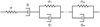Fig. 1 Spring-dashpot representation of the generalised Voigt model.

2 Rheological models

The term rheology refers to the study of flow and deformation of matter (Barnes et al. 1989). Our rheological models are based on linear viscoelastic models, meaning that the body may exhibit both viscous and elastic properties, and they establish the relationship between force and deformation in the body.

2.1 Generalised Voigt model

For each linear viscoelastic model we can associate a spring– dashpot representation (Bland 1960). This representation is composed of an association of springs and dashpots, whose most basic elements are the Maxwell element, formed by a spring and a dashpot in series, and the Voigt element, formed by a spring and a dashpot in parallel. Each model has an associated force-extension equation, which describes how a material represented by this model behaves under a tensile force. In particular, the generalised Voigt model is composed of one Maxwell element in series with m Voigt elements, as shown in Fig. 1.

The generalised Voigt model is a general model with most of the simple models used in the literature being a particular case of this one. It can indeed reproduce the linear model (e.g. Mignard 1979), the Creep model (e.g. Ferraz-Mello 2013), the Maxwell model (e.g. Correia et al. 2014), the Standard Anelas- tic Solid model (e.g. Henning et al. 2009), and the Burgers model (e.g. Faul & Jackson 2005). Furthermore, Gevorgyan et al. (2020) and Gevorgyan (2021) have shown that the Andrade model and the Sundberg-Cooper model can also be described by the generalised Voigt model to a very good approximation. Both these rheological models are based on laboratory experiments (see Sundberg & Cooper 2010 and, for example, Efroimsky 2012 and Correia & Valente 2022). In particular, the Sundberg-Cooper model fits well the rheology of fine-grained peridotite (olivine + 39 vol. % orthopyroxene) rock, which constitutes the upper mantle of Earth under ocean basins, at depths of approximately 10–400 km.

Due to the arbitrary number of elements in the model, the generalised Voigt rheology can be calibrated using any given number of relaxation times, rendering it a very complex model. In Gevorgyan et al. (2023), it is shown that a homogeneous body with a complex rheology, given by the generalised Voigt model for example, can reproduce the same tidal response as that of a multilayered body.

2.2 Force-extension equation

The force-extension equation for a rheological model can be derived via a Lagrangian formalism (see Ragazzo & Ruiz 2017, Sect. 3.1). Let us call ξ_α and ξ_η the displacement in the spring with elastic constant α and in the dashpot with viscous constant η, respectively, and ${\xi }_{e_k}$ the displacement in the k-th Voigt element (see Fig. 1). The total displacement ξ of the system is then given by $$\xi ={\xi }_{\alpha }+{\xi }_{\eta }+{\displaystyle \sum _{k=1}^m{\xi }_{e_k}}.$$(1)

Using this relation as a constraint, we can write a Lagrangian function ℒ_gV for the model’s displacement as $${ℒ}_{gV}=-\frac{\alpha {\xi }_{\alpha }^2}{2}-{\displaystyle \sum _{k=1}^m\frac{{\alpha }_k{\xi }_{e_k}^2}{2}}+\lambda \left({\xi }_{\alpha }+{\xi }_{\eta }+{\displaystyle \sum _{k=1}^m{\xi }_{e_k}}-\xi \right),$$(2)

where λ is a Lagrange multiplier that represents the force in the system, and a Rayleigh dissipation function 𝒟_gV as $${\mathcal{D}}_{gV}=\frac{\eta {\dot{\xi }}_{\eta }^2}{2}+{\displaystyle \sum _{k=1}^m\frac{{\eta }_k{\dot{\xi }}_{e_k}^2}{2}}.$$(3)

For m = 0, for instance, we have from the Euler-Lagrange equations (see, for example, Goldstein 1950) $$\frac{\partial {ℒ}_{gV}}{\partial {\xi }_{\alpha }}=\frac{\partial {\mathcal{D}}_{gV}}{\partial {\dot{\xi }}_{\alpha }}\Rightarrow -\alpha {\xi }_{\alpha }+\lambda =0,$$(4a) $$\frac{\partial {ℒ}_{gV}}{\partial {\xi }_{\eta }}=\frac{\partial {\mathcal{D}}_{gV}}{\partial {\dot{\xi }}_{\eta }}\Rightarrow \lambda =\eta {\dot{\xi }}_{\eta },$$(4b)

that, using Eq. (1), leads to $$\frac{\dot{\lambda }}{\alpha }+\frac{\lambda }{\eta }=\dot{\xi },$$(5)

which is the force-extension equation for a Maxwell element (Bland 1960).

3 Body’s deformation

In order to study the dynamics of a rigid body, it is natural to choose a reference frame in which the body is always at rest, such as the one composed by the principal moments of inertia of the body. For a deformable body, however, such a frame does not exist, but there does exist a reference frame, named Tisserand frame, in which the relative angular momentum of the body in relation to an inertial reference frame is null (see, for example, Munk & MacDonald 1960). In the theory that follows, we adopt the Tisserand frame as the body frame.

Let us consider an extended deformable body that satisfies the following conditions:

1. It is spherically symmetric at equilibrium;

2. It is only subject to small deformations;

3. Its material is incompressible under such deformations; and let I denote its inertia matrix in the Tisserand frame. Under these hypotheses, the body’s mean moment of inertia I_o, which is defined here as $${\text{I}}_{°}:=\frac{1}{3}\mathrm{Tr}(I),$$(6)

   is constant in time (Rochester & Smylie 1974).

We now use Eq. (6) to split I into an isotropic and a traceless part in the following manner² $$I={\text{I}}_{°}(\mathbb{I}-B),$$(7)

where 𝕀 is the identity matrix and B is a non-dimensional matrix that represents the body’s deformation called deformation matrix. In accordance with the conditions imposed on the body, B measures the deviation from the spherical configuration, I = I_o𝕀, and it satisfies ||B|| << 1.

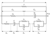Fig. 2 Rheology based on the generalised Voigt viscoelastic model with self-gravity and prestress.

3.1 The Association Principle

Let us construct the spring-dashpot representation of our rheology. We choose the generalised Voigt model as the basis, but we also add a time-dependent force F(t), and two elements in parallel: a spring with elastic constant γ, and a Maxwell element with elastic and viscosity constants given by α₀ and η₀. The first added element corresponds to the body’s self-gravity, and the second added element will be later associated with the dynamical behaviour in long timescales. In Fig. 2, we show a schematic for the body’s rheology.

As stated in Ragazzo & Ruiz (2017), the Association Principle is “a procedure to associate to each spring-dashpot model, which defines the rheology of a body, a potential and a dissipation functions for the body deformation variables”. First, we choose a rheological model, and we derive a Lagrangian function and a Rayleigh dissipation function for the variables associated with its spring-dashpot representation. Then, the recipe given by the Association Principle is the following: we construct similar functions for the body’s deformation by taking the expression for the Lagrangian and dissipation functions written for the spring-dashpot representation, replacing all the displacement variables by deformation matrices ($\xi ,{\xi }_{\alpha },{\xi }_{\eta },{\xi }_{e_k},{\xi }_{{\alpha }_0},{\xi }_{{\eta }_0}\to B,B_{\alpha },B_{\eta },B_{e_k},B_{{\alpha }_0},B_{{\eta }_0}$), replacing the Lagrange multipliers by auxiliary matrices (λ, λ₀ → Λ, Λ₀), replacing the applied force by a matrix (F → F), and rescaling both functions by I_o.

3.2 Deformation equations

After obtaining the Lagrangian and the dissipation functions for the rheology shown in Fig. 2, similarly to what was done in Sect. 2.2, and applying the Association Principle, as explained in the previous section, the resulting Lagrangian function L for the body’s deformation is given by³ $$\begin{array}{l}ℒ={\text{I}}_{°}[-\frac{\gamma \Vert B{\Vert }^2}{2}-\frac{{\alpha }_0{\Vert B_{{\alpha }_0}\Vert }^2}{2}-\frac{\alpha {\Vert B_{\alpha }\Vert }^2}{2}-{\displaystyle \sum _{k=1}^m\frac{{\alpha }_k{\Vert B_{e_k}\Vert }^2}{2}}\\ +F\cdot B+{\Lambda }_0\cdot \left(B_{{\alpha }_0}+B_{{\eta }_0}-B\right)\\ +\Lambda \cdot \left(B_{\alpha }+B_{\eta }+{\displaystyle \sum _{k=1}^m{B}_{e_k}}-B\right)],\end{array}$$(8)

and the resulting Rayleigh dissipation function D is given by $$\mathcal{D}={\text{I}}_{\text{o}}\left[\frac{{\eta }_0{\Vert {\stackrel{.}{B}}_{{\eta }_0}\Vert }^2}{2}+\frac{\eta {\Vert {\stackrel{.}{B}}_{\eta }\Vert }^2}{2}+{\displaystyle \sum _{k=1}^m\frac{{\eta }_k{\Vert {\stackrel{.}{B}}_{e_k}\Vert }^2}{2}}\right].$$(9)

Note that the holonomic constraints in the deformation variables are $$B_{{\alpha }_0}+B_{{\eta }_0}=B,$$(10a) $$B_{\alpha }+B_{\eta }+{\displaystyle \sum _{k=1}^m{B}_{e_k}}=B,$$(10b)

and that the Lagrange multipliers are now symmetric traceless matrices that still represent the force acting on their corresponding elements. Finally, we derive the following relations from the Euler-Lagrange equations $$\frac{\partial ℒ}{\partial B}=\frac{\partial \mathcal{D}}{\partial \stackrel{.}{B}}\Rightarrow F-\gamma B-{\Lambda }_0-\Lambda =0,$$(11a) $$\frac{\partial ℒ}{\partial B_{{\alpha }_0}}=\frac{\partial \mathcal{D}}{\partial {\stackrel{.}{B}}_{{\alpha }_0}}\Rightarrow {\Lambda }_0-{\alpha }_0{B}_{{\alpha }_0}=0,$$(11b) $$\frac{\partial ℒ}{\partial B_{{\eta }_0}}=\frac{\partial \mathcal{D}}{\partial {\stackrel{.}{B}}_{{\eta }_0}}\Rightarrow {\Lambda }_0={\eta }_0{\stackrel{.}{B}}_{{\eta }_0},$$(11c) $$\frac{\partial ℒ}{\partial B_{\alpha }}=\frac{\partial \mathcal{D}}{\partial {\stackrel{.}{B}}_{\alpha }}\Rightarrow \Lambda -\alpha B_{\alpha }=0,$$(11d) $$\frac{\partial ℒ}{\partial B_{\eta }}=\frac{\partial \mathcal{D}}{\partial {\stackrel{.}{B}}_{\eta }}\Rightarrow \Lambda =\eta {\stackrel{.}{B}}_{\eta },$$(11e) $$\frac{\partial ℒ}{\partial B_{e_k}}=\frac{\partial \mathcal{D}}{\partial {\stackrel{.}{B}}_{e_k}}\Rightarrow \Lambda -{\alpha }_k{B}_{e_k}={\eta }_k{\stackrel{.}{B}}_{e_k},k=1,\dots ,m.$$(11f)

Equations (11a)–(11f) are the body’s deformation equations, that can be used to derive a relation for the body’s deformation matrix and to determine the time evolution of the body’s rheological parameters.

3.3 Centrifugal and tidal forces

The term denoted by F that appears in the Lagrangian for the body’s deformation is called deformation-force matrix, and it represents the force that is being exerted in the body. It is composed of a rotational part F_cent that corresponds to the centrifugal force, and an orbital part F_tide that corresponds to the tide-raising force. For a body with angular velocity Ω in the body’s reference frame, which interacts with a system comprised of N − 1 bodies with mass M_j and at a distance X_j from said body, the force matrix is given by (see Boekholt & Correia 2023, Section 2.1.2)⁴ $$\begin{array}{l}F=F_{\mathit{cent}}+F_{\mathit{tide}}\\ =-\left(\text{Ω}{\text{Ω}}^T-\frac{\Vert \text{Ω}{\Vert }^2}{3}\mathbb{I}\right)+3G{\displaystyle \sum _{j=1}^{N-1}\frac{M_j}{{\left|X_j\right|}^5}}\left(X_j{X}_j^T-\frac{{\Vert X_j\Vert }^2}{3}\mathbb{I}\right),\end{array}$$(12)

where G is the gravitational constant.

3.4 Prestress

The second element added to our rheology was done so as to account for the residual deformation on a body after we halt its rotation and remove all external forces. By assuming that the stress in this element’s spring is finite (Λ₀ < ∞), and that the viscosity constant in this element’s dashpot is very large (η₀ → ∞), we can interpret the body’s residual deformation as a transient state with a very long transient time (see the discussion in Ragazzo et al. 2022, Sect. 4). Such reasoning makes it possible for us to introduce a permanent triaxiality to the body.

From Eq. (11c) we have $${\stackrel{.}{B}}_{{\eta }_0}=\frac{{\Lambda }_0}{{\eta }_0}\to 0\Rightarrow B_{{\eta }_0}=\text{ constant, }$$(13)

where we call $B_{{\eta }_0}$ the fossil deformation matrix. Moreover, from Eq. (11b) and the constraint in Eq. (10a), we have $${\Lambda }_0={\alpha }_0\left(B-B_{{\eta }_0}\right).$$(14)

If $B=B_{{\eta }_0}$, the spring is not stressed and the body has a constant deformation, and if B = 0, the stress is given by -$-{\alpha }_0{B}_{{\eta }_0}$. With this, we define the prestress matrix $$P\equiv {\alpha }_0{B}_{{\eta }_0}.$$(15)

The prestress matrix is then responsible for inducing a permanent deformation in the body that is not associated with the body’s rotational motion nor with tidal effects. Furthermore, the frame defined by the fossil deformation matrix, and consequently by the prestress matrix, is a Tisserand frame. We call such a frame the prestress frame.

3.5 The deformation matrix

Applying the constraint given in Eqs. (10b)–(11d), we obtain a relation for Λ, which is given by $$\Lambda =\alpha \left(B-B_{\eta }-{\displaystyle \sum _{k=1}^m{B}_{e_k}}\right).$$(16)

Finally, substituting Eqs. (14), (15) and (16) into Eq. (11a), and solving for B, we have $$B=\frac{1}{{\gamma }_0+\alpha }\left(F+P+\alpha B_{\eta }+\alpha {\displaystyle \sum _{k=1}^m{B}_{e_k}}\right),$$(17)

where we have defined γ₀ ≡ γ + α₀. We thus obtain an expression for the body’s deformation B that depends on the applied forces F, the prestress matrix P, and the state variables $B_{\eta },B_{e_1},\dots ,B_{e_m}$.

3.6 Energy dissipation

Let us call 𝒟_i the Rayleigh dissipation function associated with the i-th body. It can be shown under some conditions which are satisfied here that the time evolution of the system’s total energy E is given by (Ragazzo & Ruiz 2015) $$\dot{E}=-2{\displaystyle \sum _{i=1}^N{\mathcal{D}}_i}\le 0.$$(18)

There are two main consequences from Eq. (18). First, any bounded solution in phase space is asymptotic to a solution that does not dissipate energy, and for which $\Vert {\stackrel{.}{B}}_{\eta }\Vert =\Vert {\stackrel{.}{B}}_{e_1}\Vert =\cdots =\Vert {\stackrel{.}{B}}_{e_m}\Vert =0$ for all bodies (see Eqs. (9) and (13)). Second, we can isolate the individual contribution of each body to the decrease of energy in the entire system, which comes solely from the body’s deformation. The latter consequence is a direct advantage of the theory presented in this Section, which formally defines a Lagrangian for the deformation.

4 Equations of motion

In this Section, we lay out the full equations for the dynamics of a deformable celestial body. In order to conveniently deal with a system composed of multiple bodies, we write these equations in relation to an inertial reference frame, including the ones associated with the body’s deformation.

4.1 Reference frames

Let κ be an inertial reference frame and K be a Tisserand frame associated with the body, and let Y(t) : K → κ be the orthogonal transformation that associates K with κ. The angular velocity matrix in the inertial frame can then be written as $$\stackrel{⌢}{\mathit{\omega }}=\stackrel{.}{Y}{Y}^T,$$(19)

where $\widehat{\omega }$ is an anti-symmetric operator associated with the angular velocity vector ω via the hat map defined as⁵ $$\omega =\left(\begin{array}{l}{\omega }_1\hfill \\ {\omega }_2\hfill \\ {\omega }_3\hfill \end{array}\right)\mapsto \widehat{\omega }=\left[\begin{array}{ccc}0& -{\omega }_3& {\omega }_2\\ {\omega }_3& 0& -{\omega }_1\\ -{\omega }_2& {\omega }_1& 0\end{array}\right].$$(20)

The body’s rheology, namely the deformation matrix B and all other auxiliary matrices $B_{\eta },B_{e_1},\dots ,B_{e_m}$, and P, are defined in K. Given a variable A in this frame, we can express it in the inertial reference frame via Y in the following manner⁶ $$a=YA{Y}^T,$$(21)

and, using the definition of the angular velocity given in Eq. (19), the time derivative of this variable can be written as $$\stackrel{.}{a}=[\widehat{\mathit{\omega }},a]+Y\stackrel{.}{A}{Y}^T,$$(22)

where [] is the standard matrix commutator and $\dot{\mathbf{\text{A}}}$ is the time derivative in the Tisserand frame.

4.2 Orbital dynamics

In the inertial frame, the total potential energy due to gravitational interactions in a system composed of N extended bodies, with the i-th body located at x_i, is given by (e.g. Correia 2018) $$\begin{array}{l}{U}_g=-G{\displaystyle \sum _{i=1}^{N-1}{\displaystyle \sum _{j>i}^N\{\frac{m_i{m}_j}{\left|x_{ij}\right|}}}\\ +\frac{3}{2}\frac{1}{{\left|x_{ij}\right|}^3}\left[{\widehat{x}}_{ij}\cdot \left(m_i{I}_j+m_j{I}_i\right){\widehat{x}}_{ij}-\frac{1}{3}\mathrm{Tr}\left(m_i{I}_j+m_j{I}_i\right)\right]\},\end{array}$$(23)

where $x_{ij}=x_i-x_j,{\widehat{x}}_{ij}=x_{ij}/\left|x_{ij}\right|$, and we neglect terms in |x_ij|⁻⁴ (quadrupolar approximation). Using the inertia tensor as defined in Eq. (7), we can rewrite Eq. (23) as $$\begin{array}{l}{U}_g=-G{\displaystyle \sum _{i=1}^{N-1}{\displaystyle \sum _{j>i}^N\{\frac{m_i{m}_j}{\left|x_{ij}\right|}}}\\ +\frac{3}{2}\frac{1}{{\left|x_{ij}\right|}^5}\left[m_j{I}_{°i}\left(x_{ij}\cdot b_i{x}_{ij}\right)+m_i{\text{I}}_{°j}\left(x_{ij}\cdot b_j{x}_{ij}\right)\right]\},\end{array}$$(24)

where b is the deformation matrix B in the inertial frame (see Eq. (21)). Finally, from $m_i{\stackrel{\mathrm{..}}{x}}_i=-{\nabla }_{x_i}{U}_g$ we have $$\begin{array}{l}{\stackrel{\mathrm{..}}{x}}_i=G{\displaystyle \sum _{\begin{array}{c}j=1\\ j\ne i\end{array}}^N\{-\frac{m_j}{{\left|x_{ij}\right|}^3}{x}_{ij}}\\ -\frac{15}{2m_i}\frac{1}{{\left|x_{ij}\right|}^{\mid }}\left(\left(m_j{\text{I}}_{°i}{b}_i+m_i{\text{I}}_{°j}{b}_j\right)x_{ij}\cdot x_{ij}\right)x_{ij}\\ +\frac{3}{m_i}\frac{1}{{\left|x_{ij}\right|}^5}\left(m_j{\text{I}}_{°i}{b}_i+m_i{\text{I}}_{°j}{b}_j\right)x_{ij}\}.\end{array}$$(25)

4.3 Rotational dynamics

The gravitational torque on an extended body i due to a point mass j is given by $${\tau }_{ij}=-{\displaystyle \int r}\times {\nabla }_r\text{Φ}\left(r,x_{ij}\right)\rho (r)\text{dV},$$(26)

where r is a vector from the body’s center of mass to a point inside the body, and $$\text{Φ}\left(r,x_{ij}\right)=-\frac{G{m}_j}{\left|r+x_{ij}\right|}$$(27)

is the gravitational potential on said point due to the body j. By expanding Eq. (27) for |r| << |x_ij| up to the quadrupolar approximation and substituting the result in Eq. (26) we have $${\stackrel{.}{\mathit{\ell }}}_i={\displaystyle \sum _{\begin{array}{c}j=1\\ j\ne i\end{array}}^N{\tau }_{ij}}=-3G{\text{I}}_{°i}{\displaystyle \sum _{\begin{array}{c}j=1\\ j\ne i\end{array}}^N\frac{m_j}{{\left|x_{ij}\right|}^{\mid }}}{x}_{ij}\times b_i{x}_{ij},$$(28)

where ℓ_i is the rotational angular momentum vector of body i.

4.4 Rheological dynamics

The equations that describe the dynamics of the body’s internal rheological variables are obtained from the Euler-Lagrange equations, Eqs. (11), which were derived in Sect. 3.2. Substituting the expression for Λ, Eq. (16), into Eqs. (11e) and (11f), and transforming these equations to the inertial reference frame via Eq. (22), we obtain $${\stackrel{.}{b}}_{\eta }=\left[\widehat{\omega },b_{\eta }\right]+\frac{\alpha }{\eta }\left(b-b_{\eta }-{\displaystyle \sum _{k=1}^m{b}_{e_k}}\right),$$(29)

and $${\stackrel{.}{b}}_{e_k}=\left[\widehat{\omega },b_{e_k}\right]-\frac{{\alpha }_k}{{\eta }_k}{b}_{e_k}+\frac{\alpha }{{\eta }_k}\left(b-b_{\eta }-{\displaystyle \sum _{k^{\prime }=1}^m{b}_{e_{k^{\prime }}}}\right),$$(30)

with k = 1,…, m.

4.5 Tisserand frame dynamics

The dynamics of the Tisserand frame are determined by the body’s rotation, as stated in Eq. (19). Hence it can be described by a rotation quaternion (see, for example, Betsch & Siebert 2009).

The time evolution of a rotation quaternion s = (s₀, s) = (s₀, s₁, s₂, s₃) is given by $$\dot{s}=\frac{1}{2}(0,\mathit{\omega })°s,$$(31)

where ○ stands for quaternion product⁷. The rotation matrix Y can then be obtained via a transformation from the rotation quaternion to a Direction Cosine Matrix in the following manner (e.g. Bernardes & Viollet 2022) $$Y=\left[\begin{array}{ccc}{s}_0^2+s_1^2-s_2^2-s_3^2& 2\left(s_1{s}_2-s_0{s}_3\right)& 2\left(s_1{s}_3+s_0{s}_2\right)\\ 2\left(s_1{s}_2+s_0{s}_3\right)& s_0^2-s_1^2+s_2^2-s_3^2& 2\left(s_2{s}_3-s_0{s}_1\right)\\ 2\left(s_1{s}_3-s_0{s}_2\right)& 2\left(s_2{s}_3+s_0{s}_1\right)& s_0^2-s_1^2-s_2^2+s_3^2\end{array}\right].$$(32)

5 Numerical code

The open-source software presented in this work is called RheoVolution, which stands for Rheology evolution in the time domain. It simulates the orbital and rotational motion of N interacting extended bodies using the equations of motion described in Sect. 4. The user can consider each body as a point mass, a rigid body, or a deformable body, where both the centrifugal and tidal forces can be set independently, with a rheology given by the generalised Voigt model (Sect. 2). Furthermore, the user can also assign a permanent deformation (triaxiality) to each body, which is given by the prestress formulation.

In its current version, the code is written entirely in the c programming language, and it uses the GNU Scientific Library (GSL) for some tasks such as numerical integration of ODEs, matrix diagonalization, and linear systems solving (Galassi et al. 2001). The project contains a Makefile to compile and help run the code, and it is publicly available⁸.

5.1 Input and output

The user provides as input the initial orbital and rotational configuration and also the physical and rheological parameters for each body, which are needed to set and initialize the N -body system, as well as the parameters used in the numerical integration scheme. In particular, the positions of the bodies are provided using orbital elements with the first body as the central one. The user also determines if each body is to be treated as a point mass, as a rigid triaxial body, or as a deformable body, and, in the latter case, if both the centrifugal and tidal effects are to be taken into consideration.

The time evolution for the phase space variables, as well as for the orbital elements, orientation angles, and dissipation function of each body, is printed as output from the program. Furthermore, the total angular momentum of the system, given by $${\mathit{\ell }}_T={\displaystyle \sum _{i=1}^N{\mathit{\ell }}_i}+m_i{x}_i\times {\stackrel{.}{x}}_i,$$(33)

is also provided as an output. From Eqs. (25) and (28), we can show that ${\dot{\mathit{\ell }}}_T=0$, that is, the total angular momentum is conserved. Therefore, it can be used as a measure of the code’s precision.

5.2 Determining the prestress matrix

In order to determine P, we examine the case where the forces are static $F=\overline{F}$, and the body is at equilibrium $B=\overline{B}$. In this situation, the deformation in the spring whose elastic constant is given by α is null (which is equivalent to Λ = 0), and from Eqs. (16) and (17) we have $$P={\gamma }_0\overline{B}-\overline{F}.$$(34)

The prestress matrix P can thus be interpreted as the remainder between the stress on a body and the forces applied to it. $\overline{B}$ is the real deformation, which can be determined from the Stokes coefficients of the gravitational potential, and $\overline{F}$ is the average deformation force which can be decomposed in two terms: an average centrifugal force and an average tidal force. For more information, see Appendices A and B.

The prestress formulation also provides a natural manner in which to represent the rigid body case, achieved when γ₀ → ∞. From Eqs. (17) and (34), we obtain in this case $$\underset{{\gamma }_0\to \infty }{\lim }B=\underset{{\gamma }_0\to \infty }{\lim }\frac{1}{{\gamma }_0}P=\overline{B}.$$(35)

5.3 Inertial and Tisserand frames

All parameters entered by the user are defined in relation to a given reference frame which is the same for all bodies, and we take this reference frame as our inertial frame. More precisely, the x-y plane of the inertial frame is the reference plane to which the orbital inclination of all bodies is defined, and the orientation of the inertial plane is such that its x-axis is aligned with the reference direction to which the ascending node is defined. The origin of the inertial frame is then set at the initial location of the system’s center of mass.

The body frame is chosen as follows. First, if the body is not initially spherical, we calculate its principal moments of inertia, and we align them with the axis of the inertial reference frame. This is the basis where the real deformation matrix is diagonal (see Appendix A). Then, we rotate the frame, along with the body, according to the orientation angles given by the user. If there’s prestress in the body, this procedure also defines the location of the prestress frame (see Sect. 3.4).

5.4 Program functioning

Our code numerically integrates Eqs. (25), (28), (29), (30) (if applicable), and (31) for each one of the N bodies, using as default an explicit embedded Runge-Kutta Prince-Dormand 7(8) scheme with adaptive step size (Prince & Dormand 1981). The maximum step size, which also determines the frequency of output data, is either given by the user or determined by the program, which automatically calculates the shortest timescale in the simulation. The initial step size is then set as a fifth of the maximum step size.

The equations of motion depend on both $\stackrel{⌢}{\omega }$ and b, which are calculated at each time step in the following manner. By using the definition of a Tisserand frame, and the relation between angular velocity and angular momentum, we can write $$\widehat{\mathit{\omega }}=\frac{\widehat{\ell }}{{\text{I}}_{°}}-(b\widehat{\mathit{\omega }}+\widehat{\mathit{\omega }}b),$$(36)

where $b=b(\stackrel{⌢}{\omega })$. Additionally, we can separate the body’s deformation into a centrifugal, a tidal, a prestress, and a rheological contribution (see Eqs. (12) and (17)) $$b=b_{\mathit{cent}}+b_{\mathit{tide}}+b_{\mathit{pres}}+b_{\mathit{rheo}},$$(37)

where $$\begin{array}{l}{b}_{\mathit{cent}}=\frac{1}{{\gamma }_0+\alpha }\left[-\omega {\mathit{\omega }}^{\text{T}}+\frac{|\mathit{\omega }{|}^2}{3}\mathbb{I}\right],\\ b_{\mathit{tide}}=\frac{3G}{{\gamma }_0+\alpha }{\displaystyle \sum _{\begin{array}{c}j=1\\ j\ne i\end{array}}^N\frac{m_j}{{\left|x_{ij}\right|}^5}}\left(x_{ij}{x}_{ij}^{\text{T}}-\frac{{\left|x_{ij}\right|}^2}{3}\mathbb{I}\right),\\ b_{\mathit{pres}}=\frac{1}{{\gamma }_0+\alpha }p,\\ b_{\mathit{rheo}}=\frac{\alpha }{{\gamma }_0+\alpha }\left[b_{\eta }+{\displaystyle \sum _{k=1}^m{b}_k}\right].\end{array}$$

By applying Eq. (37) to Eq. (36), we arrive at an expression for the angular velocity that can be solved via Newton’s method using the value of $\stackrel{⌢}{\omega }$ at the previous time step as seed⁹. Finally, by plugging this solution back into Eq. (37), we can calculate the body’s deformation.

It is important to note that b possesses a prestress component that depends on the prestress matrix p. According to Eqs. (13) and (15), this matrix is constant in the body’s frame. Therefore, we can simply use Eqs. (21) and (32) to calculate it at each time step via $$p(t)=Y(t)P\left(t_0\right)Y^T(t).$$(38)

Similarly, when dealing with a rigid body, we can calculate the time evolution of the real deformation matrix in the inertial reference frame via $$\overline{b}(t)=Y(t)\overline{B}\left(t_0\right)Y^T(t),$$(39)

which corresponds to the body’s deformation matrix b in this case (see Eq. (35)).

When numerically integrating the equations of motion, we also take into consideration that the matrices b_η and $b_{e_k}$ , for k = 1,…, m, are all traceless and symmetric, which means that we only need 5 elements each to specify them. Furthermore, since $\stackrel{⌢}{\omega }$ is anti-symmetric, the commutator of $\stackrel{⌢}{\omega }$ with the aforementioned matrices are also traceless symmetric matrices. These matrices are initialized by the program as to guarantee that the initial deformation of the body is given by the real deformation (see Appendix A).

6 Examples

In this section, we demonstrate a set of classical examples in the Solar System using our software. In each example, we discuss on the calibration of the rheological parameters, which is always done via the Love number, defined in Sect. 6.1. All the main information provided as input to the code and used in the numerical simulations are given in Table 1. In all cases, the numerical integrator’s time step is chosen between a half and a tenth of the smallest timescale in the system, depending on the total simulation time.

6.1 Love number

The deformation of a planet’s external gravitational potential due to a perturbing potential is usually modelled by the second Love number for potential, k₂ (Love 1927). This quantity takes values in the complex plane, and while |k₂| gives the amplitude of the tidal deformation, Im k₂ is related to the phase lag between the perturbation and the deformation, hence being associated to energy dissipation (see, for example, Correia & Rodriguez 2013).

In the tidal theory presented in Sect. 3, the Love number relates to an arbitrary rheological model via (Ragazzo & Ruiz 2017)¹⁰ $$k_2(\sigma )=\frac{3G{\text{I}}_{°}}{R^5}\frac{1}{{\gamma }_0+J^{-1}(\sigma )},$$(40)

where J is a complex compliance. For the generalised Voigt model with m = 0 (see Sect. 2), which is known as the Maxwell model, we have $$J(\sigma )=\frac{1}{\alpha }+\frac{1}{i\sigma \eta }.$$(41)

Concomitantly, we can write the Love number of a Maxwell solid (see Correia & Valente 2022, Sect. 2.7.3) as (Darwin 1907) $$k_2(\sigma )=k_0\frac{1+i\sigma {\tau }_e}{1+i\sigma \tau },$$(42)

where τ_e is the Maxwell relaxation time, τ = τ_e + τ_v with τ_v the viscous time, σ is a perturbing frequency, and k₀ is the Love number at σ = 0. By substituting Eq. (41) into Eq. (40), and then comparing it to Eq. (42), we find a simple relation between the Love number parameters and the parameters of the rheology’s spring-dashpot representation $${\gamma }_0=\frac{3G{\text{I}}_{°}}{R^5{k}_0},\eta ={\gamma }_0\left(\tau -{\tau }_e\right),\alpha =\frac{\eta }{{\tau }_e}.$$(43)

For the generalised Voigt model with m , 0, we have $$J(\sigma )=\frac{1}{\alpha }+\frac{1}{i\sigma \eta }+{\displaystyle \sum _{k=1}^m\frac{1}{{\alpha }_k+i\sigma {\eta }_k}}.$$(44)

Due to the extra terms in the generalised Voigt rheology, the relation between the Love number parameters and the rheological parameters is more cumbersome than the one given by the Maxwell rheology. However, it is in principle always possible to calibrate the system if k₂ is known for a sufficient number of perturbing frequencies.

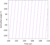Fig. 3 Spin axis nutation for a solid Earth.

6.2 Rotational dynamics of an isolated Earth

Our first example concerns the rotational motion of the Earth without external gravitational fields perturbing its dynamics. We focus our investigation on two effects: Chandler wobble and true polar wander, both of which are a consequence of the misalignment between Earth’s spin and figure axes.

6.2.1 Solid Earth

We start by considering the Earth as a triaxial rigid body, which is a possible setting of the program. In this scenario, the Earth does not experience any deformation and, therefore, there is no elastic response nor energy dissipation. We set an initial tilt to Earth’s spin axis in relation to its figure axis of approximately 0.145 seconds of arc, which corresponds to 4.5 meters on the Earth’s surface (Lang 1992).

In Fig. 3, we express the Earth’s angular velocity in the body’s reference frame in spherical coordinates, and we show the time evolution of its azimuthal angle (associated with the x- y plane) for a period of ten years. We set the starting time at 100 years to filter out the transient effects at the beginning of the simulation. The observed periodic motion corresponds to Earth’s free nutation, since the system is being treated here as isolated, and has a value of approximately 304 days, which is consistent with a value of about 10 months (see Munk & MacDonald 1960, Chapter 6).

6.2.2 Earth’s rheology calibration via Chandler wobble

The Earth’s deformation increases the period of free nutation to a value of approximately 433 days (Vondrák et al. 2017), which is known as Chandler wobble (see Munk & MacDonald 1960). We will use this effect to calibrate our rheology.

Let us consider a Maxwell rheology for the Earth (m = 0), and let’s assume k₀ = 0.9 ≲ k_f = 0.934 (Lambeck 2005)¹¹. The real part of Earth’s Love number k₂ at the Chandler wobble frequency σ_CW can be estimated for a body of revolution and with negligible gravitational torque by (see Ragazzo et al. 2022, Eq. (6.19))¹² $$\mathrm{Re}{k}_2\left({\sigma }_{CW}\right)\approx \frac{3{\text{I}}_{°}G}{{\omega }^2{R}^5}\left({\overline{\alpha }}_e-\frac{{\sigma }_{CW}}{\omega }\right)\approx 0.28389,$$(45)

where ${\overline{\alpha }}_e$ is the Earth’s flatness. The imaginary part of the Love number at the Chandler wobble frequency can be taken from Fig. 10 of Ragazzo et al. (2022), Im k₂(σ_CW) = −0.002.

From Eq. (42), we have $$\mathrm{Re}{k}_2(\sigma )=k_0\frac{1+{\sigma }^2{\tau }_e\tau }{1+{\sigma }^2{\tau }^2}\text{\hspace{1em} and \hspace{1em}}\mathrm{Im}{k}_2(\sigma )=-k_0\frac{\sigma {\tau }_v}{1+{\sigma }^2{\tau }^2}.$$(46)

With the values of k₀, σ_CW, Re k₂(σ_CW), and Im k₂(σ_CW), we can use Eq. (46) to obtain Earth’s relaxation and viscous times, and later use Eq. (43) to obtain Earth’s rheological parameters calibrated using the Chandler wobble. The results are presented in Table 2.

6.2.3 Deformable Earth

By adopting the previously calculated rheological parameters and performing the same analysis done for the solid Earth, we now obtain a nutation period of approximately 434 days. Furthermore, given the Earth’s triaxial shape and the energy dissipation due to its deformation, its largest moment of inertia axis moves in relation to Earth’s spin axis, and the system tends to a dynamical equilibrium where both axes are aligned, a phenomenon known as true polar wander (e.g. Goldreich & Toomre 1969). We can observe this event in Figure 4, where we plot the angle between such axes as a function of time using a centered moving average of about 11 years to filter out small oscillations. For the calibration used in this example, the timescale for alignment is approximately 250 years.

6.3 Moon’s orbital motion for a deformable Earth

Our second example concerns the orbital motion of the Moon. Here, we consider the Earth-Moon system, with the Earth as a deformable body and the Moon as a point mass. Furthermore, we assume that the Moon is orbiting Earth’s equator in a circular orbit with orbital mean motion n, while the Earth spins with angular velocity Ω_E. Under these conditions, we can show that the total energy in the system is given by (see Ragazzo & Ruiz 2017, Sect. 6.4) $$E(d)=\frac{1}{2}\left({\text{I}}_{\text{o}}{\text{Ω}}_E^2(d)-\frac{G{m}_E{m}_M}{d}\right),$$(47)

where d is the Earth-Moon distance.

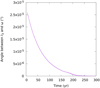Fig. 4 Angle between Earth’s rotation axis and largest moment of inertia vector.

6.3.1 Earth’s rheology calibration via lunar recession

The main contribution to the Moon’s orbital drift of about 3.82 ± 0.07 cm/yr (Dickey et al. 1994) is the energy loss caused by the Earth’s response to the tides exerted by the Moon at the semi-diurnal frequency σ_SD = 2(Ω_E(d) − n(d)). As discussed in Sect. 6.1, energy dissipation is associated with the imaginary part of the second Love number k₂(σ). The time-average dissipation of tidal energy W is given by (see Ragazzo & Ruiz 2017, Eq. (47)) $$W\left(\mathrm{Im}{k}_2\left({\sigma }_{SD}\right)\right)=g(d){\sigma }_{SD}\mathrm{Im}{k}_2\left({\sigma }_{SD}\right),$$(48)

where $$g(d)=-\frac{3}{4}\frac{G{m}_M^2{R}^5}{d^6}.$$

On the other hand, the energy dissipation can be derived via Eq. (47) as $\dot{E}=h(d)\dot{d}$, where $$h(d)=\frac{1}{2}\frac{G{m}_E{m}_M}{d^2}-\mu \sqrt{\frac{GM}{d}}{\text{Ω}}_E(d),$$

with M = m_E + m_M the total mass and µ = m_Em_M/M the reduced mass. Finally, from $\dot{E}=-W$ we have $$\mathrm{Im}{k}_2\left({\sigma }_{SD}\right)=-\frac{h(d)}{g(d)}\frac{\dot{d}}{{\sigma }_{SD}}.$$(49)

Assessing Eq. (49) with the current values for the EarthMoon mean distance d, and the measured semi-major axis growth $\dot{d}$, we obtain Im k₂(σ_SD) = −2.55978 × 10⁻². The real part of the Love number at the semi-diurnal frequency can be obtained from Petit et al. (2010) (see Ragazzo et al. 2022, Table 1), and it is given by Re k₂(σ_SD) = 0.2811.

As in the previous example, we choose a Maxwell rheology for the Earth and we assume k₀ = 0.9. Following the same transformations as before, Eqs. (46) and (43), we obtain Earth’s rheological parameters calibrated at the semi-diurnal frequency using Moon’s orbital drift. The results are presented in Table 3.

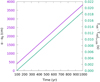Fig. 5 Evolution of the semi-major axis in the Earth-Moon system (purple) and Earth’s rotation period (green).

6.3.2 Moon’s orbital drift and Earth’s rotational deceleration

Figure 5 shows the Moon’s semi-major axis as a function of time for the Earth-Moon system (purple curve) under the aforementioned considerations and for the parameters calculated in the previous section. From the slope of the curve, we obtained a growth of about 3.818 cm/yr.

The Moon’s orbital drift is a consequence of the conservation of the system’s total angular momentum. As energy is dissipated in the Earth due to tidal forces, its spinning slows down and, as a consequence, the orbit of the Moon enlarges. In Figure 5, we also plot the Earth’s period of rotation as a function of time (green curve), which shows a growth of about 2.084 × 10⁻³ s/century, and from where we can observe the rotational deceleration of the Earth’s spin.

6.4 Earth’s rheology calibration via two or more distinct dynamical phenomena

In Sections 6.2 and 6.3, we implicitly used the centrifugal deformation of the Earth, plus the deformation due to the prestress, to set a value for k₀ . Hence, due to the number of free parameters in the model, the Maxwell rheology could only be calibrated using one additional dynamical effect. If we wanted to calibrate Earth’s response using both the Chandler wobble and the Moon’s orbital drift at the same, a more complex rheological model would be necessary. In this situation, we can use the generalised Voigt model with m = 1, which is known as the Burgers model.

The derivation of the rheological parameters for such a model follows the same procedure as was done for the Maxwell model. Substituting the complex compliance with m = 1, Eq. (44), into the Love number expression, Eq. (40), and comparing it to the Love number for a Maxwell solid, Eq. (42), we arrive at a set of equations which relates the Love number parameters to the parameters of the rheology. We can then use the information in the previous sections, namely, the values of k₀, σ_CW , Re k₂(σ_CW), Im k₂(σ_CW), σ_SD, Re k₂(σ_SD), and Im k₂(σ_SD), and solve this set of equations via Newton’s method for a suitable seed. The results are presented in Table 4.

With the Burgers model, we are able to reproduce both dynamical effects using the same rheology. Figures 6 and 7 show the modulus and the imaginary part of the Love number k₂ as a function of the perturbing frequency σ, respectively. In both plots, the values used to calibrate our rheology are marked by green dots.

It follows that we can always choose m in the generalised Voigt model according to the number of dynamical phenomena we are interested in, making the rheology as complex as needed. As long as we know the perturbing frequency associated with each effect, and we can estimate the values of the real and the imaginary part of the Love number at these frequencies, we can try and calibrate the rheological parameters by substituting Eq. (44) with the adequate m into Eq. (40), comparing it to Eq. (42), and numerically solving the resulting equation.

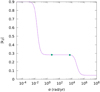Fig. 6 Modulus of Earth’s Love number.

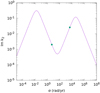Fig. 7 Imaginary component of Earth’s Love number.

6.5 Rotational dynamics of a deformable Moon

Our third example concerns the rotational motion of the Moon in the Sun-Earth-Moon system. We consider here the Earth and the Sun as point masses, and the Moon as a triaxial deformable body.

We assume a Maxwell rheology for the Moon which can be calibrated using the quality factor¹³ Q = 46 and the absolute value of the complex Love number |k₂| = 0.00236 at the sidereal rotation period T = 27.32 days, both taken from Ragazzo et al. (2022), Table 8, via (see, for example, Efroimsky 2012) $$Q(\sigma )=\frac{1}{\sin \delta (\sigma )},\text{\hspace{1em} where }\delta (\sigma )=-\arctan \frac{\mathrm{Im}{k}_2(\sigma )}{\mathrm{Re}{k}_2(\sigma )},$$(50)

and using γ₀ = γ + α₀ with γ = (2π/1.992 h)² and α₀ = (2π/0.2575 h)², both taken from Ragazzo et al. (2022), Table 9¹⁴. Finally, from Eqs. (46) and (43), we obtain the values given in Table 5 for the Moon’s rheological parameters.

6.5.1 Spin-orbit resonance

The Moon is currently tidally locked in a synchronous spinorbit resonance, meaning that its orbital period and its rotational period are the same on average. In Fig. 8, we show the ratio between the Moon’s rotational frequency ωrot and its orbital frequency $${\mathit{\omega }}_{\mathit{orb}}=\frac{x_{ME}\times {\stackrel{.}{x}}_{ME}}{{\left|x_{ME}\right|}^2},\text{\hspace{1em} where \hspace{1em}}{x}_{ME}=x_{\mathit{Earth}}-x_{\mathit{Moon}},$$

for a time span of 5 Myr. We obtain a moving average of approximately 1.003.

The Moon’s hemisphere which faces Earth librates due to the Moon’s slightly eccentric and inclined orbit, and also to its orientation in space. To observe this phenomenon, we look at the time-evolution of the Moon’s spin-orbit angle, defined here as the angle between the direction of the Moon’s lowest principal moment of inertia I₁ , and the direction of the Moon’s position relative to the Earth x_ME . As we can see in Fig. 9, the Moon’s spin-orbit angle oscillates around zero, with a range of ±8.5°.

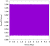Fig. 8 Ratio between the Moon’s rotational and orbital frequencies.

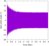Fig. 9 Evolution of Moon’s spin-orbit angle.

6.5.2 Moon’s obliquity

The Moon is in a Cassini state (see, for example, Colombo 1966) and, consequently, its obliquity has a constant value of approximately 6.68° (Williams 2016). In Fig. 10 we show the evolution of the Moon’s obliquity for a time interval of 5 Myr using two initial conditions: θ (t = 0) = 0° (green) and θ (t = 0) = 10° (purple). In both situations, the obliquity converges to a value of approximately 6.55°.

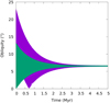Fig. 10 Moon’s stabilization in the Cassini state 2.

7 Conclusion and perspectives

In this work, we present an open-source software developed for evolving a system composed of N extended interacting bodies in time while taking into consideration permanent triaxiality and a complex rheology for each body. The rheological model we use here is based on the generalised Voigt model for viscoelastic materials, which is a generalization of, and can be reduced to, many models applied in the literature, such as the linear model and the Maxwell model. Our program then differentiates itself from other software such as REBOUNDx (Lu et al. 2023), which uses the constant- Q and linear models, and TIDYMESS (Boekholt & Correia 2023), which uses the linear and Creep models, by being able to reproduce more refined dynamical phenomena.

We have tested our code against various examples that served as benchmarks for the program functionalities. It is important to stress that, although our examples focus on the Earth-Moon system, the program can be applied to all the remaining bodies in the Solar System, as well as to extrasolar systems. Possible future improvements to our code include the addition of new integration schemes and the implementation of a graphical user interface. Furthermore, all new theory developments are planned to be implemented accordingly. As a final remark, this paper also works as a summary of the extensive theory developed for treating tidal models in the time domain.

Acknowledgements

V.M.O. would like to thank Tomaz Vieira for his comments and suggestions regarding the software and Timothée Vaillant for helpful discussions regarding the manuscript. C.R. also thanks Alain Albouy, Gwe- naël Boué, AUCANI-Universidade de São Paulo, the French Consulate in São Paulo, and the Observatoire de Paris, where part of this work has been done. We acknowledge the Laboratory for Advanced Computing at University of Coimbra (https://www.uc.pt/lca) and the Laboratory for Applied Mathematics at the University of São Paulo (https://labmap.ime.usp.br) for providing the resources to perform the numerical simulations. This work was partially supported by the São Paulo Research Foundation (FAPESP, Brazil), under Grants No. 2016/25053-8, 2021/11306-0, 2022/12785-1, and 2023/070764, and by Fundação para a Ciência e a Tecnologia (FCT, Portugal), under projects UIDP/04564/2020 (https://doi.org/10.54499/UIDP/04564/2020) and UIDB/04564/2020 (https://doi.org/10.54499/UIDB/04564/2020).

Appendix A Real deformation

The transformation between the gravity potential terms and the elements of the inertia tensor are (see, for example, Correia & Rodriguez 2013) $$\begin{array}{l}{r}_g=\frac{I_{33}}{m{R}^2},J_2=\frac{2I_{33}-I_{11}-I_{22}}{2m{R}^2},C_{22}=\frac{I_{22}-I_{11}}{4m{R}^2},\\ C_{21}=-\frac{I_{13}}{m{R}^2},S_{21}=-\frac{I_{23}}{m{R}^2},S_{22}=-\frac{I_{12}}{2m{R}^2},\end{array}$$(A.1)

where m and R are the mass and the mean radius of the body, respectively. From Eqs. (7) and (A.1), we can now write the deformation matrix in terms of the Stokes coefficients (see Boué 2020, Eq. (6)) $$B_s=\frac{1}{3r_g-2J_2}\left[\begin{array}{ccc}{J}_2+6C_{22}& 6S_{22}& 3C_{21}\\ 6S_{22}& J_2-6C_{22}& 3S_{21}\\ 3C_{21}& 3S_{21}& -2J_2\end{array}\right].$$(A.2)

Since we choose the Tisserand frame at t = t₀ to coincide with the reference frame formed by the body’s principal moments of inertia (see Sect. 4.1), we set the real deformation as the one given by the Stokes coefficients in such a frame $$\overline{B}=P^{-1}{B}_{s}P,$$(A.3)

where P is an eigenvectors matrix which, following the definition in Eq. (7), also diagonalizes the inertia tensor.

Appendix B Mean deformation force

The mean deformation force F can be decomposed into a centrifugal component and a tidal component (see Ragazzo et al. 2022, Sect. 4.1) $$\overline{F}={\overline{F}}_{\mathit{cent}}+{\overline{F}}_{\mathit{tide}}.$$(B.1)

Let us now choose the body frame aligned with the principal axes of the body. In this situation, both components of Eq. (B.1) are diagonal matrices. The mean centrifugal force matrix is then given by the Average-Maclaurin operator $${\overline{F}}_{\mathit{cent}}=\frac{{\text{Ω}}^2}{3}\left[\begin{array}{ccc}1& 0& 0\\ 0& 1& 0\\ 0& 0& -2\end{array}\right],$$(B.2)

where Ω is the body’s angular velocity in this frame.

Here, we consider that the mean centrifugal force is much larger than the mean tidal force, $\Vert {\overline{F}}_{\mathit{cent}}\Vert \gg >\Vert {\overline{F}}_{\mathit{tide}}\Vert \approx 0$, and, consequently, $\overline{F}\approx {\overline{F}}_{\mathit{cent}}$ . If needed, however, the effect of the mean tidal force can be added by the user via the Stokes coefficients, which define the mean deformation of the body (see Eq. (A.2)).

References

All Tables

All Figures

	Fig. 1 Spring-dashpot representation of the generalised Voigt model.
In the text

	Fig. 2 Rheology based on the generalised Voigt viscoelastic model with self-gravity and prestress.
In the text

	Fig. 3 Spin axis nutation for a solid Earth.
In the text

	Fig. 4 Angle between Earth’s rotation axis and largest moment of inertia vector.
In the text

	Fig. 5 Evolution of the semi-major axis in the Earth-Moon system (purple) and Earth’s rotation period (green).
In the text

	Fig. 6 Modulus of Earth’s Love number.
In the text

	Fig. 7 Imaginary component of Earth’s Love number.
In the text

	Fig. 8 Ratio between the Moon’s rotational and orbital frequencies.
In the text

	Fig. 9 Evolution of Moon’s spin-orbit angle.
In the text

	Fig. 10 Moon’s stabilization in the Cassini state 2.
In the text

References

- Barnes, H., Hutton, J., & Walters, K. 1989, An Introduction to Rheology (Amsterdam: Elsevier Science), 3 [Google Scholar]
- Bernardes, E., & Viollet, S. 2022, PLOS one, 17, e0276302 [Google Scholar]
- Betsch, P., & Siebert, R. 2009, Int. J. Numer. Methods Eng., 79, 444 [NASA ADS] [CrossRef] [Google Scholar]
- Bland, D. 1960, The Theory of Linear Viscoelasticity (Amsterdam: Elsevier Science & Technology) [Google Scholar]
- Boekholt, T. C., & Correia, A. C. 2023, MNRAS, 522, 2885 [Google Scholar]
- Boué, G. 2020, Celest. Mech. Dyn. Astron., 132, 21 [CrossRef] [Google Scholar]
- Boué, G., & Efroimsky, M. 2019, Celest. Mech. Dyn. Astron., 131, 1 [CrossRef] [Google Scholar]
- Colombo, G. 1966, AJ, 71, 891 [Google Scholar]
- Correia, A. C. 2018, Icarus, 305, 250 [NASA ADS] [CrossRef] [Google Scholar]
- Correia, A. C. M., & Delisle, J.-B. 2019, A&A, 630, A102 [NASA ADS] [CrossRef] [EDP Sciences] [Google Scholar]
- Correia, A. C., & Rodriguez, A. 2013, ApJ, 767, 128 [NASA ADS] [CrossRef] [Google Scholar]
- Correia, A. C., & Valente, E. F. 2022, Celest. Mech. Dyn. Astron., 134, 24 [NASA ADS] [CrossRef] [Google Scholar]
- Correia, A. C., Boué, G., Laskar, J., & Rodríguez, A. 2014, A&A, 571, A50 [NASA ADS] [CrossRef] [EDP Sciences] [Google Scholar]
- Correia, A., Ragazzo, C., & Ruiz, L. 2018, Celest. Mech. Dyn. Astron., 130, 1 [NASA ADS] [CrossRef] [Google Scholar]
- Darwin, G. H. 1879, Proc. R. Soc. Lond., 29, 168 [Google Scholar]
- Darwin, G. 1907, Scientific Papers (Cambridge: Cambridge University Press Archive), 1 [Google Scholar]
- Dickey, J. O., Bender, P., Faller, J., et al. 1994, Science, 265, 482 [Google Scholar]
- Efroimsky, M. 2012, Celest. Mech. Dyn. Astron., 112, 283 [NASA ADS] [CrossRef] [Google Scholar]
- Efroimsky, M., & Lainey, V. 2007, J. Geophys. Res.: Planets, 112, E12003 [NASA ADS] [CrossRef] [Google Scholar]
- Faul, U. H., & Jackson, I. 2005, Earth Planet. Sci. Lett., 234, 119 [CrossRef] [Google Scholar]
- Ferraz-Mello, S. 2013, Celest. Mech. Dyn. Astron., 116, 109 [Google Scholar]
- Galassi, M., Gough, B., Rossi, F., et al. 2001, GNU Scientific Library: Reference Manual (UK: Network Theory Limited) [Google Scholar]
- Gevorgyan, Y. 2021, A&A, 650, A141 [NASA ADS] [CrossRef] [EDP Sciences] [Google Scholar]
- Gevorgyan, Y., Boué, G., Ragazzo, C., Ruiz, L. S., & Correia, A. C. 2020, Icarus, 343, 113610 [NASA ADS] [CrossRef] [Google Scholar]
- Gevorgyan, Y., Matsuyama, I., & Ragazzo, C. 2023, MNRAS, 523, 1822 [Google Scholar]
- Goldstein, H. 1950, Classical Mechanics (Boston: Addison-Wesley) [Google Scholar]
- Goldreich, P., & Peale, S. 1966, AJ, 71, 425 [NASA ADS] [CrossRef] [Google Scholar]
- Goldreich, P., & Toomre, A. 1969, J. Geophys. Res., 74, 2555 [CrossRef] [Google Scholar]
- Gomes, S. R., & Correia, A. C. 2023, A&A, 674, A111 [NASA ADS] [CrossRef] [EDP Sciences] [Google Scholar]
- Goossens, S., Lemoine, F., Sabaka, T., et al. 2016, in 47th Annual Lunar and Planetary Science Conference No. 1903, 1484 [Google Scholar]
- Henning, W. G., O’Connell, R. J., & Sasselov, D. D. 2009, ApJ, 707, 1000 [Google Scholar]
- Lainey, V., Casajus, L. G., Fuller, J., et al. 2020, Nat. Astron., 4, 1053 [Google Scholar]
- Lambeck, K. 2005, The Earth’s Variable Rotation: Geophysical Causes and Consequences (Cambridge: Cambridge University Press) [Google Scholar]
- Lang, K. R. 1992, Astrophysical Data: Planets and Stars (New York: Springer) [CrossRef] [Google Scholar]
- Lemoine, F. G., Goossens, S., Sabaka, T. J., et al. 2014, Geophys. Res. Lett., 41, 3382 [Google Scholar]
- Love, A. E. H. 1927, A Treatise on the Mathematical Theory of Elasticity (New York: Dover) [Google Scholar]
- Lu, T., Rein, H., Tamayo, D., et al. 2023, ApJ, 948, 41 [NASA ADS] [CrossRef] [Google Scholar]
- MacDonald, G. J. F. 1964, Rev. Geophys., 2, 467 [Google Scholar]
- Mignard, F. 1979, Moon Planets, 20, 301 [Google Scholar]
- Munk, W., & MacDonald, G. 1960, The Rotation of the Earth: a Geophysical Discussion, Cambridge monographs on mechanics and applied mathematics (Cambridge: Cambridge University Press) [Google Scholar]
- Pavlis, N. K., Holmes, S. A., Kenyon, S. C., & Factor, J. K. 2008, An Earth Gravitational Model to Degree 2160: EGM2008, presented at the 2008 General Assembly of the European Geosciences Union, Vienna, Austria, April 13-18 [Google Scholar]
- Pavlis, N. K., Holmes, S. A., Kenyon, S. C., & Factor, J. K. 2012, J. Geophys. Res. Solid Earth, 117, 1 [Google Scholar]
- Petit, G., Luzum, B., et al. 2010, IERS Technical Note, 36 [Google Scholar]
- Prince, P. J., & Dormand, J. R. 1981, J. Comput. Appl. Math., 7, 67 [CrossRef] [Google Scholar]
- Ragazzo, C., & Ruiz, L. 2015, Celest. Mech. Dyn. Astron., 122, 303 [NASA ADS] [CrossRef] [Google Scholar]
- Ragazzo, C., & Ruiz, L. S. 2017, Celest. Mech. Dyn. Astron., 128, 19 [NASA ADS] [CrossRef] [Google Scholar]
- Ragazzo, C., Boué, G., Gevorgyan, Y., & Ruiz, L. S. 2022, Celest. Mech. Dyn. Astron., 134, 10 [NASA ADS] [CrossRef] [Google Scholar]
- Rochester, M., & Smylie, D. 1974, J. Geophys. Res., 79, 4948 [CrossRef] [Google Scholar]
- Rodríguez, A., Callegari, N., & Correia, A. C. M. 2016, MNRAS, 463, 3249 [Google Scholar]
- Schwarz, R. 2017, Memorandum nº6 Quaternions and Spatial Rotation, https://www.rene-schwarz.com, accessed: 2024-02-07 [Google Scholar]
- Sundberg, M., & Cooper, R. F. 2010, Philos. Mag., 90, 2817 [Google Scholar]
- Valente, E. F., & Correia, A. C. 2022, A&A, 665, A130 [NASA ADS] [CrossRef] [EDP Sciences] [Google Scholar]
- Vondrák, J., Ron, C., & Chapanov, Y. 2017, Adv. Space Res., 59, 1395 [CrossRef] [Google Scholar]
- Williams, D. R. 2016, NASA NSSDCA Planetary Fact Sheets, https://nssdc.gsfc.nasa.gov/planetary/planetfact.html, accessed: 2024-08-29 [Google Scholar]
The presence of internal waves in fluid planets, neglected in Correia et al. (2018), may require modifications to be made in the model under certain circumstances, as described in Lainey et al. (2020).
By definition, B relates to the gravitational quadrupole moment Q via
The matrix operations are defined as
whereT stands for matrix transpose.
The components of F can also be derived from the rotational and gravitational Lagrangians. See Ragazzo & Ruiz (2017), Eqs. (34) and (35).
For a list of formulas involving vectors, matrices, and the hat operator see Ragazzo et al. (2022), Table 2.
To help with text clarity, we have defined the following whenever applicable. If a variable is described in a Tisserand frame we write it using capital letters, and if it is described in an inertial reference frame we write it using small case letters.
The quaternion product between two quaternions  is defined by
where <, > and × are the canonical inner and cross product for vectors, respectively. For a comprehensive list of operations involving quaternions, see Schwarz (2017).
The default number of iterations for Newton’s method is 5. If a certain tolerance precision is not reached after this, the integration is stopped by the program and a warning is issued to the user.
There is an additive term in the denominator of the expression for k2 given by Eq. (40) due to the inertia deformation that was shown in Correia et al. (2018) to be negligible.
kf is the fluid Love number (e.g. Munk & MacDonald 1960).
In Ragazzo et al. (2022), the mean moment of inertia is written as  is due to the mantle and
is due to a fluid core. Here we do not distinguish between the rotational motion of the mantle and the core so we use Eq. (6.19) in Ragazzo et al. (2022) with
.
The quality factor Q is a dimensionless measure of the tidal dissipation defined as the peak energy stored during one forcing period over the total energy dissipated during this period (Correia & Valente 2022).
These parameters were calibrated for a simple rheology (see Ragazzo et al. 2022, Fig. 1) that is equivalent to the Maxwell model in the regime η/α << 1.
All Tables
Earth’s rheological parameters calibrated via both Chandler wobble and Moon’s orbital drift.