| Issue |
A&A
Volume 699, July 2025
|
|
|---|---|---|
| Article Number | A132 | |
| Number of page(s) | 18 | |
| Section | Catalogs and data | |
| DOI | https://doi.org/10.1051/0004-6361/202453330 | |
| Published online | 02 July 2025 | |
Spectroscopic quasar anomaly detection (SQuAD)
I. Rest-frame UV spectra from SDSS DR16
1
Indian Institute of Science Education and Research,
Bhopal,
Madhya Pradesh
462066,
India
2
Indian Institute of Astrophysics,
100 Feet Rd, Santhosapuram, 2 nd Block, Koramangala,
Bengaluru,
Karnataka,
India
★ Corresponding authors: This email address is being protected from spambots. You need JavaScript enabled to view it.
; This email address is being protected from spambots. You need JavaScript enabled to view it.
Received:
6
December
2024
Accepted:
10
May
2025
Abstract
Aims. We present the results of applying anomaly detection algorithms to a quasar spectroscopic subsample from the SDSS DR16 quasar catalog, covering the redshift range of 1.88 ≤ z ≤ 2.47.
Methods. A principal component analysis (PCA) was employed for the dimensionality reduction of the quasar spectra, followed by a hierarchical k-means clustering in a 20-dimensional PCA eigenvector hyperspace. To prevent broad absorption line (BAL) quasars from being identified as the primary anomaly group, we conducted separate analyses on BAL and non-BAL quasars (a.k.a. QSOs), comparing both classes for a clearer identification of other anomalous quasar types.
Results. We identified 2066 anomalous quasars, categorized into 10 broadly defined groups. The anomalous groups include: C IV peakers: quasars with extremely strong and narrow C IV emission lines; Excess Si IV emitters: quasars where the Si IV line is as strong as the C IV line; and Si IV deficient anomalies: which exhibit significantly weaker Si IV emission compared to typical quasars. The anomalous nature of these quasars is attributed to lower Eddington ratios for C IV peakers, supersolar metallicity for Excess Si IV emitters, and subsolar metallicity for Si IV deficient anomalies. Additionally, we identified four groups of BAL anomalies: blue BALs, flat BALs, reddened BALs, and FeLoBALs, distinguished primarily by the strength of reddening in these sources. Furthermore, among the non-BAL quasars, we identified three types of reddened anomaly groups classified as heavily reddened, moderately reddened, and plateau-shaped spectrum quasars, each exhibiting varying degrees of reddening. We present the detected anomalies as an accompanying value-added catalog.
Key words: catalogs / galaxies: active / galaxies: nuclei / quasars: general
© The Authors 2025
 Open Access article, published by EDP Sciences, under the terms of the Creative Commons Attribution License (https://creativecommons.org/licenses/by/4.0), which permits unrestricted use, distribution, and reproduction in any medium, provided the original work is properly cited.
This article is published in open access under the Subscribe to Open model. This email address is being protected from spambots. You need JavaScript enabled to view it. to support open access publication.
1 Introduction
Active galactic nuclei (AGNs) that are characterized as quasars are highly luminous galactic cores powered by gas accreting onto a supermassive black hole, emitting radiation across the entire electromagnetic spectrum (Shakura & Sunyaev 1973). They emit radiation through various physical mechanisms contributing to their broadband spectrum. Thermal emission from the accretion disk includes X-rays from hot inner regions and optical/UV light from cooler outer areas. Synchrotron radiation, produced by relativistic electrons spiraling in magnetic fields, is prominent in radio-loud AGNs and spans radio waves to X-rays. Bremsstrahlung radiation occurs when electrons decelerate near ions, emitting X-rays significant in hot gas regions such as the corona or narrow-line region (NLR). Inverse Compton scattering in the corona boosts low-energy photons to higher energies via interactions with high-energy electrons, contributing to X-ray and gamma-ray emissions (see, e.g., Begelman et al. 1984; Haardt & Maraschi 1991; Koratkar & Blaes 1999, for a review).
The UV spectrum of an AGN often follows a power-law distribution, expressed as Fν ∝ ν−α, where the spectral index, α typically ranges from 0.5 to 1.5. The power-law continuum arises from the superposition of multiple blackbody spectra emitted by the accretion disk’s varying radial temperature zones. Additionally, the UV emission exhibits strong emission and absorption lines with broad and narrow components, often modeled using double or single Gaussian profiles. These lines involve ions such as C IV, Si IV, Al III, Mg II, and He II. They serve as key diagnostics of the physical conditions in the AGN’s environment (e.g., Zheng et al. 1997; Brotherton et al. 2001; Harris et al. 2016).
Due to the multiple physical processes involved, quasars exhibit a wide range of properties that can differ greatly from one quasar to another, or even over time within the same quasar (e.g., Wilhite et al. 2005; Vivek et al. 2012a,b; LaMassa et al. 2015; Green et al. 2022). In UV spectra, features such as the spectral slope and the strength of emission lines display significant variability among quasars. Processes such as gravitational lensing and obscuration by gas clouds along the line of sight also contribute to this spectral variability (e.g., Wiklind & Combes 1996).
Several past studies have revealed the presence of a variety of unusual quasar spectra that deviate significantly from the standard SED such as the Vanden Berk et al. (2001) composite. Such studies have also confirmed the existence of unusual or anomalous quasar types. For instance, Plotkin et al. (2008) presented a sample of unusual BL Lac objects analytically selected from SDSS DR5, while Diamond-Stanic et al. (2009) identified a sample of 74 high-redshift quasars (z > 3) with weak emission lines from the SDSS DR5 and Hines et al. (2001) analyzed two unusually spectro-polarized QSOs. Artymowicz (1993) studied the AGN metallicity as a function of unusual star formation activities at high redshifts. Two “extraordinarily red” quasars have been found and their dust reddening is characterized by Gregg et al. (2002) from the Faint Images of the Radio Sky at Twenty-centimeters (FIRST) survey. Collin et al. (2002) studied the disc dynamics and supermassive blackhole (SMBH) mass of a quasar population with super-Eddington accretion. Hall et al. (2002) identified 23 unusual broad absorption line (BAL) quasars with diverse properties, including a quasar with the most recorded absorption lines and others with complex Mg II absorption patterns. Additionally, they found rare cases of low-ionization broad absorption line (LoBAL) quasars and iron low-ionization broad absorption-line (FeLoBAL) quasars with strong Fe II emissions, along with unique cases of Fe III absorption without Fe II. Studying unusual quasar spectra is important as it can reveal physical processes or environmental factors that are not apparent in typical quasars. These unusual characteristics may result from enhanced mechanisms such as star formation, accretion activity, reprocessed emission, outflows, or feedback. By examining these outliers, we can gain valuable insights into the diversity of quasar properties and improve our understanding of the underlying physics governing quasars.
With the massive number of quasars being discovered every day, it is likely to miss out on an extremely interesting or rare object that might get covered in the pile of data being pumped by survey telescopes all around the world. Machine learning serves as a golden tool in this scenario as it can be used to quickly pick out anomalous or weird-behaving objects (quasars in this case) from all of the “normal” samples. Several studies have focused on detecting peculiar objects from large datasets, with some specifically using spectra for anomaly detection. For example, Meusinger et al. (2012) identified around 1000 spectroscopically unusual quasars in SDSS DR7 using Kohonen Maps, while Reis et al. (2021) evaluated the effectiveness of various outlier detection algorithms applied to SDSS galactic spectra. Similarly, Solarz et al. (2020) extracted a sample of spectroscopic anomalies from the All-Sky Wide-field Infrared Survey Explorer (AllWISE) Sky Survey.
The high dimensionality and complexity of astronomical spectral data hinder the effective application of anomaly detection algorithms. In such cases, a principal component analysis (PCA) can offer a robust method for dimensionality reduction. This technique transforms the original spectral features into a lower dimensional space, retaining the most critical variance in the data. The efficiency of PCA in preprocessing data for clustering algorithms such as k-means is well-established. PCA enhances the clustering process by reducing noise and irrelevant variations, allowing k-means to operate more effectively on transformed data. Several pioneering studies have demonstrated the power of PCA in analyzing quasar spectra. Francis et al. (1992) introduced one of the first objective classification schemes for quasar spectra using PCA, highlighting its ability to extract dominant spectral components. Boroson & Green (1992) conducted one of the earliest systematic applications of PCA in quasar studies, identifying two principal components that encapsulate the primary variations in quasar spectra. Their analysis revealed that the first principal component correlates strongly with the strength of Fe II emission and [O III] λ5007, defining an “eigenvector 1” parameter space that later became fundamental in quasar classification and AGN unification models. This pioneering work demonstrated the power of PCA in reducing the complexity of quasar spectra, while preserving key physical correlations and laying the groundwork for subsequent studies in quasar spectral analysis. Yip et al. (2004) expanded upon this by applying PCA to a large sample of Sloan Digital Sky Survey (SDSS) quasars, demonstrating how eigenspectra capture variations due to redshift and luminosity. Suzuki (2006) further refined the approach by focusing on PCA-based classification of quasar emission lines in the Lyα forest, enabling a better understanding of quasar spectral diversity. Pâris et al. (2011) applied PCA to high-redshift quasar spectra, revealing significant variations in UV spectral properties, while Ma et al. (2019) used PCA to analyze the Hβ region of low-redshift SDSS quasars, providing insights into the spectral diversity of broad-line regions (BLRs).
Beyond quasar classification, PCA has proven to be an effective tool for anomaly detection in large-scale astronomical datasets. Xiong et al. (2018) and Henrion et al. (2013) demonstrated that PCA-based feature extraction improves clustering performance by filtering out noise and focusing on the most informative spectral variations. By transforming spectra into a lower dimensional representation, PCA allows anomaly detection algorithms to operate more efficiently, distinguishing rare or unusual sources from the general population. These studies collectively highlight the importance of PCA not only in quasar spectral analysis, but also in facilitating robust anomaly detection methodologies in large astrophysical datasets.
In this study, we applied a hierarchical k-means clustering approach to detect and analyze spectroscopic anomalies in quasars from the Sloan Digital Sky Survey: Sixteenth Data Release Quasar (SDSS DR16Q) catalog (Lyke et al. 2020). We chose the k-means algorithm due to its interpretability, which makes it easier to identify which characteristics of the data contribute to cluster formation. While more sophisticated algorithms might offer marginal improvements in clustering accuracy, they are often computationally expensive and more challenging to interpret, making k-means a balanced choice for efficient and meaningful analysis. K-means works effectively when combined with PCA, which reduces the dimensionality of the data, keeping only the most important variance. By leveraging PCA for dimensionality reduction, we are able to distill essential features from the high-dimensional spectral data, enhancing the ability of the k-means method to identify anomalous quasar spectra. The clustering process groups similar spectra, allowing for the detection of outliers within each cluster, which are considered anomalous. Given the large sample size, hierarchical clustering further refines the data into subgroups with distinct and consistent property trends, enabling a more detailed analysis of quasar spectral anomalies.
The Spectroscopic Quasar Anomaly Detection (SQuAD) project aims to detect spectroscopically anomalous quasars from large-scale spectroscopic surveys and conduct follow-up studies on the most interesting cases. This paper is the first in a series, with a focus specifically on identifying these anomalies in the rest-frame UV spectra from the SDSS DR16Q catalog.
The present paper is organized as follows: In Sect. 2, we describe the sample selection, data reduction, cleaning procedures, and dimensionality reduction using PCA. In Sect. 3, we cover our clustering techniques, including k-means and its hierarchical application, along with the methods we used for determining the optimal number of clusters. In Sect. 4, we present our main findings, with visual representations of the detected anomalies. In Sect. 5, we categorize the identified anomalies and discuss the observable properties of each group, as well as the implications for the physical properties of the quasars. Finally, Sect. 6 summarizes our findings.
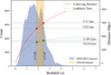 |
Fig. 1 Redshift distribution of quasars in the SDSS DR16 catalog (blue) and the selected subset of quasars (yellow) within the specified redshift range, 1.88 ≤ z ≤ 2.47. The red dashed curve represents the comoving distance, while the green dotted curve shows the lookback time as a function of redshift. The corresponding distance and time values at two key redshifts: z = 1.88 and z = 2.47, are marked. |
2 Data
The spectral data for this project were obtained from the SDSS DR16Q catalog, which contains 750 414 quasars in the redshift range from 0 < z ≤ 7.1. The spectra were obtained using the SDSS and Baryon Acoustic Oscillation Spectroscopic Survey (BOSS) spectrographs from the SDSS survey, covering wavelengths from 3600 to 10 400 Å (with good throughput between 3650 and 9500 Å) and a resolution of 1560–2270 in the blue channel and 1850–2650 in the red channel (Smee et al. 2013).
Our goal is to identify anomalous quasar spectra in this dataset. To facilitate outlier detection, we defined a “similarlooking” sample space by restricting the rest-frame wavelength range of all spectra to 1250–3000 Å. This range captures four prominent emission lines typical of quasar spectra: Si IV λ1400 Å, C IV λ1549 Å, C III λ1909 Å, and Mg II λ2798 Å (see Vanden Berk et al. 2001). With the BOSS spectrograph’s wavelength coverage of [3600, 10 400] Å, our wavelength window translates to a redshift range of z ∈ [1.88, 2.47], as shown in Fig. 1, where the yellow shaded region marks the selected sample.
Initially, our analysis included all 81 780 quasars (comprising ~13% of the DR16Q population) within the specified redshift range. However, this led to a systematic issue where broad absorption line (BAL) quasars were predominantly identified as anomalies, as discussed in Sect. 5. Additionally, running the algorithm on the complete dataset resulted in impure groups that needed several cleaning steps to achieve homogeneous properties amongst the group members. To address this, we conducted our analysis using two disjoint datasets: (a) BAL dataset comprising 26 557 BAL quasars from the sample and (b) non-BAL dataset, containing 55 223 non-BAL quasars. The BAL quasars were selected based on the keyword “BAL PROB” value being greater than or equal to 0.5 (Guo & Martini 2019). Additionally, a signal-to-noise ratio of S/N ≥ 4, value of the “IS_QSO_FINAL” parameter = 1, and no ZWARNING flag was required for all included quasar spectra.
2.1 Data preprocessing
The quasar spectra from SDSS contain observed flux (ergs/cm2/s/Å) distributed logarithmically on a wavelength (Å) scale. Given the wide range of redshift, we first corrected all spectra to the rest frame using the equation: ![Mathematical equation: $\[\lambda_{0}=\frac{\lambda_{\text {obs }}}{z+1}\]$](/articles/aa/full_html/2025/07/aa53330-24/aa53330-24-eq1.png) , where λ0 is the rest wavelength, λobs is the observed wavelength, and z is the quasar redshift. The rest frame spectra underwent a four step preprocessing procedure (to remove noise and artifacts and prepare them for the clustering algorithm), which included the following steps chronologically:
, where λ0 is the rest wavelength, λobs is the observed wavelength, and z is the quasar redshift. The rest frame spectra underwent a four step preprocessing procedure (to remove noise and artifacts and prepare them for the clustering algorithm), which included the following steps chronologically:
Resampling: The raw spectra were resampled following the method of Carnall (2017) to bring all spectra onto a common wavelength grid, specifically 1250 to 3000 Å, and trim off the excess wavelengths. This resampling also reduced the data size by a factor of 2. A typical SDSS spectrum, originally with a flux array length of around 4000, was reduced to approximately 850 points after resampling with 2 Å binning. This significantly lowered computational costs without compromising the quality of the information retained by the spectra.
Smoothing: The resampled spectra were smoothed using a Savitzky–Golay filter (Savitzky & Golay 1964), with a window length of five pixels and a third-degree polynomial. This method effectively reduced noise without altering the length or overall shape of the spectral array. However, it did not remove artifacts like extremely narrow spikes in the spectra, which are often caused by cosmic ray hits or system-induced errors, as discussed by Newman et al. (2004).
Normalization: The resampled and smoothed spectra were normalized using the maximum flux value (e.g., Liu et al. 2011), as described in Equation (1), thereby adjusting the flux value range for all spectra to [−1, 1]. This normalization reduced the likelihood of the algorithm identifying a spectrum as an outlier based on extreme flux, whether high or low, expressed as
![Mathematical equation: $\[\left(F_{normalized}\right)_\lambda=\frac{F_\lambda}{max \left(\{F_\lambda\right\})}.\]$](/articles/aa/full_html/2025/07/aa53330-24/aa53330-24-eq2.png) (1)
(1)Padding and gap correction: As previously discussed, all spectra were shifted to their rest wavelengths and resampled onto a common wavelength grid spanning 1250–3000 Å for standardization. Due to the varying redshift values (z), not all spectra naturally cover this entire wavelength range. Consequently, any flux outside this range was excluded, and gaps at both ends were filled by padding with the trailing flux value. This procedure ensured that all spectra had uniform dimensions, which is essential for the anomaly detection algorithms. We had 717 spectra with extended regions of missing flux values. To “repair” these, we applied an iterative PCA-based gap-filling method (following Yip et al. 2004) to reconstruct missing (now padded) spectral data. First, we computed the eigenspectra by performing PCA on the available complete (a spectrum with no missing flux values) spectra, capturing the dominant variance structure. Missing regions in the 717 spectra are then iteratively reconstructed by projecting each spectrum onto the eigenspectra and refining the estimates until convergence. This approach preserves the statistical integrity of the spectra, while minimizing the reconstruction bias.
We initially attempted to utilize the AND and OR masks to obtain a clean spectrum. However, these methods proved ineffective as they removed large portions of the spectra, leading to detection as anomalies due to the missing chunks. Instead, a simple rebinning and Savitzky-Golay (Sav-Gol) smoothing approach, as discussed earlier, was more effective in eliminating bad pixels and producing a cleaner spectrum.
Similarly, we also tried using median normalization, median filtering to remove cosmic rays, and various rebinning methods but could not match the performance of the currently adopted methodology. For example, median normalization reduced the explained PCA variance to 79% (instead of the current 94.9%). The large noise in the continuum, especially in the low-S/N spectra, distributes the variance across a larger number of components, reducing the variance captured by the first few principal components in PCA. Fig. 2 shows a typical spectrum before (in blue) and after preprocessing (black).
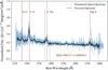 |
Fig. 2 Example quasar spectrum showing the max-normalized flux before (blue) and after preprocessing (black). Note: the preprocessing effectively reduces noise without altering the overall spectral shape. |
2.2 Principal component analysis
As discussed by Sánchez Almeida et al. (2010), a spectrum can be represented as a vector in a high-dimensional space with as many unit vectors as the wavelength grid and the flux values being the coefficients for these unit vectors. Therefore, the quasar spectral catalog can be considered as a set of vectors in this space with well-defined (Euclidean) distances between each vector pair. Since the performance of k-means clustering is inversely proportional to the number of dimensions in which the clustering is performed (e.g., Napoleon & Pavalakodi 2011), we applied a PCA to reduce the dimensions of the spectra from ~850-dimensional wavelength-flux hyperspace to a 20 dimension PCA eigenvector hyperspace. The number of components was chosen such that we obtain a cumulative explained variance of about 95%, which was achieved with 20 PCA components. This accounted for 94.9% of the total variance, as depicted in Fig. 3. Since the total explained variance by the PCA was high enough, we decided to retain all the spectra irrespective of their reconstruction error. In Fig. B.1 of the appendix, we show the 20 eigenvectors from the PCA decomposition, which represent the principal components capturing the most significant variance in the dataset. These components are crucial for understanding the underlying structure of the quasar spectra, as they highlight key recurring patterns. Among the 20 PCA components, it is note-worthy that the second PCA eigenvector captures the reddening component of a given spectra as evident from its steep positively sloped shape (see component 2, Fig. B.1 in the appendix). Therefore, if a quasar has a high coefficient for the second PCA eigenvector (PCA 2), it indicates a greater amount of reddening. In other words, the PCA 2 coefficient is directly proportional to the level of reddening in the spectrum.
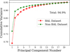 |
Fig. 3 Cumulative variance as a function of the PCA components for the PCA decomposition with 20 components, for both the BAL (red) and non-BAL (green) datasets. In both cases, a total explained variance of 94.9% is achieved with 20 PCA components. |
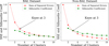 |
Fig. 4 Sum of squared errors (SSE) and silhouette coefficients as a function of cluster numbers for the BAL (left) and non-BAL (right) datasets. The optimal number of clusters is determined using both the elbow (knee) method and the silhouette coefficient for both datasets. The knee of the SSE curve occurs at three for both datasets. |
3 Clustering
K-means clustering (e.g., Bradley & Fayyad 1998) was employed to categorize quasars based on the Euclidean distances between their eigenvectors in a 20-dimensional PCA coefficient space. The algorithm initiates by selecting k random eigenspectra from the dataset, assuming these to be the centroids of distinct clusters. Subsequently, all spectra in the sample are assigned to the nearest centroid according to Euclidean distance. The cluster centroids are then recalculated as the mean of the spectra within each cluster. This iterative process continues until the cluster memberships stabilize, with no spectra re-assigned in two consecutive iterations. The final output comprises k cluster centroids and the classification of each spectrum into one of the k clusters. K-means is well-suited to large datasets due to its simplicity and efficiency. However, the algorithm requires the user to input a predefined number of clusters, k. Instead of assuming this number based on prior knowledge, we calculated it explicitly using the elbow method on the sum of squared errors (SSE) and silhouette coefficients (e.g., Syakur et al. 2018), as shown in Fig. 4. The “knee” or elbow was found using the Kneed Python module, which utilizes the Kneedle algorithm (Satopaa et al. 2011) to find the point of maximum curvature, which in a well behaved clustering problem, represents the optimum number of clusters for the distribution. The elbow method determines the optimal number of clusters by identifying the point of maximum curvature in the SSE plot. This “elbow” indicates where increasing the number of clusters yields minimal improvements in reducing error. Based on this analysis, k = 3 is obtained as the optimum number of clusters for both of our datasets. Detailed cluster visualizations are presented in Sect. 4.1. The number of quasars present in each cluster is given in Table 1.
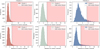 |
Fig. 5 Histograms show the distribution of the Euclidean distance of each point from its respective cluster centroid for the BAL (top panel) and non-BAL (bottom panel) datasets respectively. The red shaded region marks the respective threshold limits (Q3 + 1.5 × IQR; see Sect. 3.1). Quasars falling within the shaded region are identified as anomalous quasars. |
Number of quasars in each cluster for both datasets.
3.1 Anomaly detection
After assigning data points to the three clusters, we computed the Euclidean distance of each point from its respective cluster centroid and analyzed the resulting distribution. Typically, spectra with coefficients similar to the majority (considered “normal” spectra) are positioned close to their cluster centroid. To characterize the underlying type of each cluster’s distance distribution, we performed a comprehensive statistical analysis. First, we visualized the data using histograms (see Fig. 5) and Q–Q plots to assess normality. We then applied formal statistical tests, including the Kolmogorov-Smirnov, Anderson-Darling, and Shapiro–Wilk tests, to evaluate deviations from a normal distribution (e.g., see Razali et al. 2011). These tests consistently indicated that the data does not follow a normal distribution.
To identify the best-fitting distribution, we fit multiple candidate distributions, such as normal, exponential, gamma, Weibull, and Gumbel, using a maximum likelihood estimation (e.g., see Cousineau et al. 2004). We then compared their goodness-of-fit using the Akaike Information Criterion (AIC; see Bozdogan 1987), selecting the model with the lowest AIC as the best representation of the data. The results showed that all the distributions were Gumbel long-tailed spreads, with a significant skew toward higher values.
Given this long-tailed nature, we adopted the interquartile range (IQR) method for outlier marking, which is robust to skewed and non-normal distributions (as noted by Seo 2006; Schwertman et al. 2004; Hubert & Van der Veeken 2008, etc). For each subset of data, we compute the first (Q1) and third quartiles (Q3) and determine the IQR as IQR = Q3 − Q1. Any data points exceeding Q3 + 1.5 × IQR are classified as outliers. By setting an upper bound at Q3 + 1.5 × IQR, we effectively identify extreme values while accounting for the natural asymmetry in the data. The histograms in Fig. 5 visualize the distribution of distances within each cluster, with the outlier threshold marked by a dashed line and shaded region, highlighting extreme values beyond the computed upper bound.
We obtained a total of 1291 and 1226 anomalies in the BAL dataset and non-BAL dataset respectively. From hereon, we refer to the quasars in these samples as “anomalous quasars.”
3.2 Anomaly grouping
Visual inspection of the anomalous spectra revealed recurring characteristics, such as extremely sharp and narrow C IV peaks, as well as defects like faulty spectra. To further investigate these anomalies and derive statistical insights, we re-applied k-means clustering only on the “anomalous quasars” sample identified in Sect. 3.1, to group the anomalous spectra into similar clusters, following the methodology outlined in Sects. 2.2 and 3. For both datasets, the 20-component PCA accounted for approximately 97% of the variance. Using the elbow method, the optimal number of clusters was determined to be four for the anomalies of both the datasets (see Fig. 6). Hence, we grouped the anomalies of both the datasets into four groups each. This k-mean clustering ensured that similar anomalies are placed in the same group irrespective of which cluster they belong to.
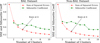 |
Fig. 6 Sum of squared errors (SSE) and silhouette coefficients as a function of cluster numbers for the k-means clustering of anomalous quasars in the BAL and non-BAL datasets. The knee of the SSE curve occurs at four for both datasets, which coincides with the maxima of the silhouette coefficient. |
3.3 Secondary anomaly grouping
For both the datasets, the results showed that out of the four groups formed, two – Group 1 (G1) and Group 4 (G4) – were identified as “pure” groups. Here, a “pure” group refers to a population where all members exhibit the same distinct anomaly trend or feature, without further variation or subdivision within the group. In other words, every quasar in Group 1 shares the same anomaly: a relatively flat, weak continuum with a sharply peaked and narrow C IV emission line. Similarly, all quasars in Group 4 display a strongly sloped blue continuum with C IV and Si IV emission lines of nearly equal strength.
On the other hand, based on a visual inspection, Group 2 (G2) and Group 3 (G3) of both the datasets were found to be consisting of a diverse sub-variety within the group. For instance, in the BAL dataset, G2 and G3 could be divided into two sub-groups each while in the non-BAL dataset, G2 and G3 showed potential to be divided into two and three subgroups each, respectively. Consequentially, we ran a k-means clustering individually, on G 2 and G3 of both the datasets. Fig. A.1 in appendix presents a flowchart outlining the steps followed by our algorithm, starting from quasar sample selection and progressing through to the final identified anomaly groups.
4 Results
It is important to note that, hereafter, the three classifications resulting from the initial k-means clustering on the entire dataset are referred to as “clusters”, while the classifications of anomalous spectra from the subsequent k-means clustering are referred to as “groups”.
4.1 Clusters
As shown in Fig. 3, the first three principal components account for nearly all the explained variance. Therefore, the k-means clusters are visualized by plotting the first two PCA coefficients. The top panel of Fig. 7 shows the three clusters identified by the initial clustering algorithm, visualized in the PCA 1 versus PCA 2 coefficient space for both the BAL dataset (left) and the non-BAL dataset (right). The outliers identified as described in Sect. 3.1 are highlighted in black in the same panel. For both datasets, clusters 1 and 2 appear relatively compact with distinct boundaries along both axes, while cluster 3 shows a broader spread, particularly along the second PCA eigenvector. This spread along the second eigenvector (which captures spectral reddening) is more pronounced in the BAL dataset, indicating larger populations of reddened quasars in case of BAL QSOs.
Some anomalies may appear to be “within” the clusters in the 2D visualization; however, this is a result of projecting the 20-dimensional hyperspace onto two dimensions. Points assigned to two distinct clusters that appear to overlap in the 2D projection may actually be distant from each other in the higher-dimensions, thereby qualifying as outliers in the full dimensional space.
To better understand the basis of clustering, we created mean or composite spectra (e.g., Vanden Berk et al. 2001) for each cluster, which highlight the average spectral properties of the members in each cluster, as shown in the bottom panel of Fig. 7. This plot provides a visual representation of why the quasars were classified into three distinct categories.
The mean spectrum of cluster 1 in both the datasets is nearly identical. This is because, the strong C IV emission line overshadows the effect of high-ionization broad absorption lines present in the quasars of the BAL dataset. Even when compared to the Vanden Berk et al. (2001) composite (see inset plots in the bottom panels of Fig. 7), both spectra appear nearly identical with subtle deviations between 1300–1600 Å, where the cluster 1 composite of the BAL dataset shows more continuum absorption which can be attributed to the absorption in the BAL QSOs. Compared to the Vanden Berk et al. (2001) composite spectra, the mean spectrum of cluster 1 shows a significantly strong C IV emission line while rest of the emissions appear fairly similar to those in the Vanden Berk et al. (2001) composite.
The mean cluster 2 spectra of both the datasets are nearly identical to each other as well as to the Vanden Berk et al. (2001) composite. This shows that most of the quasars in this group are fairly “normal” looking, which is evident by the central position of the group in the PCA hyperspace. Similarly to cluster 1, here also the BAL composite shows slightly more continuum absorption in the same wavelength window.
On the other hand, the composite spectra of cluster 3 for both datasets shows significant deviation. The mean BAL cluster 3 spectra exhibits strong reddening, exhibiting a flat continuum and significantly less flux at shorter wavelengths, as compared to the other cluster means and the Vanden Berk et al. (2001) composite. This is evident in the normalized inlay in the bottom panels of Fig. 7. The mean spectrum of cluster 3 for the non-BAL dataset is much bluer as compared to its counterpart in the BAL dataset. This can be attributed to the presence of reddened BAL QSOs and FeLoBAL quasars in the cluster 3 of BAL dataset, which are known for their strong absorption features and red continua (see Sect. 5.4).
Number of anomalies in each cluster for both datasets.
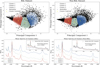 |
Fig. 7 Top: 2D projection (PCA 1 versus PCA 2 coefficients) of the BAL (left) and non-BAL (right) datasets. Each dataset is divided into three clusters (cluster 1: brown, cluster 2: green, cluster 3: blue) within the 20-dimensional PCA hyperspace, using k-means clustering. Quasars classified as anomalous after applying a Q3 + 1.5 × IQR threshold are shown as black scatter points overlayed on top of the cluster members. The cluster centroids are marked by yellow crosses. Bottom: mean composite spectrum for each cluster of the BAL (left) and non-BAL (right) datasets. The color of each spectrum corresponds to the color of the cluster as shown in the top panel. The inset plot shows the mean cluster spectra normalized at λ = 2797 Å with the Vanden Berk et al. (2001) composite. The number of anomalies present in each cluster is given in Table 2. |
4.2 Groups
As detailed in Sect. 3.2, k-means clustering was reapplied to the detected anomalies (points marked in black in the top panel of Fig. 7), resulting in the formation of four groups for the BAL and non-BAL datasets. The visualization of these anomaly groups (excluding cluster members) using the first two PCA coefficients is presented in the top panel of Fig. 8, while the bottom panel displays corresponding composite spectra for each group. The colors of each spectrum in the bottom panel of Fig. 8 are chosen to match the color scheme in the top panel. Additionally, we compared individual anomalous spectra against cluster and group composites, to ensure that spectra in a group are similar.
As discussed earlier in this paper, G1 and G4 of each dataset were found to be pure while G2 and G3 were divided into subgroups (Sect. 3.3). It was found that G 2 contained of a mixture of LoBAL QSOs and HiBAL QSOs with relatively flat spectra, and reddened BAL QSOs with strong positively sloped continua. On the other hand, G3 consisted of heavily reddened BAL QSOs along with extreme cases of FeLoBALs. Similarly, G2 and G3 of the non-BAL dataset also exhibited a scope of further classification with possible sub-groups like heavily reddened, moderately reddened, Si IV deficient QSOs etc. The subgroups created as a result of this “secondary grouping” are as follows:
BAL dataset
Group 2: Flat BAL QSOs and reddened BAL QSOs;
Table 3Number of anomalies in each group for both datasets.
Group 3: Reddened BAL QSOs and FeLoBALs;
non-BAL dataset
Group 2: Si IV d Deficient QSOs and heavily reddened QSOs;
Group 3: Heavily reddened QSOs, moderately reddened QSOs, and plateau-shaped QSOs.
The exact number of anomalies in each group is given in Table 3. Based on these composite group spectra, the four groups created by the second k-means clustering can be organized as follows.
4.2.1 Group 1
This group features quasars with an extremely sharp and narrow C IV emission line, consistently identified across both BAL and non-BAL datasets. They occupy the same location in the PCA 1 versus PCA 2 plot for both datasets, specifically in the leftmost region of the distribution, marked by blue dots in the top panel of Fig. 8. Hereafter, this group will be referred to as C IV peakers. Notably, this group also contains contaminant quasar spectra (~350) characterized by a sharp, narrow artifact peak – likely caused by cosmic ray encounters – which mimics the properties of the narrow C IV peak, leading to coincident grouping. These cosmic ray anomalies are easily removed by placing an upper cut on the C IV equivalent width (EW) and flux (λ1549 Å) since C IV peakers are known to have relatively high C IV EW and flux (see Sect. 5.1) conveniently separating them from the cosmic ray anomalies. After removing the artifacts, there are a total of 299 (169 BAL and 130 non-BAL) C IV Peaker anomalies that account for 0.36% of the total selected quasars and represents approximately 12.94% of the total detected anomalies. The only difference between the C IV peakers of the BAL and non-BAL dataset is the presence of a subtle broad-absorption line blueward of the C IV emission in the anomalies of BAL dataset.
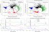 |
Fig. 8 Top: 2D projection (PCA 1 versus PCA 2 coefficients) of the anomalies of the two datasets as divided into four groups each (group 1: blue, group 2: black, group 3: green, group 4: red) in the 20 dimensional PCA hyperspace, by the second k-means clustering applied only on the anomalous quasars. The groups as characterized by further analysis (see Sect. 5) are circled and labelled to reflect the nature of their anomaly. Bottom: mean composite spectrum of each anomaly group for both the datasets. The colors of the spectra correspond to the color of the corresponding group in the top panel. |
4.2.2 Group 2
For both the datasets, Group 2 is marked by black scatter dots, and is located in the top-most region of the PCA 1 versus PCA 2 plot (see top panels of Fig. 8). These large values of PCA 2 coefficients are indicative of strong reddening in the spectra of Group 2 quasars.
BAL dataset: This group is depicted by the black scatter in the top-left panel of Fig. 8, located in the top-most region of the PCA distribution. The high PCA 2 coefficients indicate presence of strong reddening and a relatively redder spectrum. Consequently, these quasars are characterized by a either a flat or a strongly upward-sloping continuum with prominent low and high ionization absorption lines. Upon secondary k-means clustering (Sect. 3.3) these quasars are divided into two sub-groups: (1) Flat BALs: BAL quasars with a relatively flat continuum. About 80% of flat BALs are low-ionization BALs (LoBALs), which are BAL quasars that feature absorption lines from low-ionization species like Mg II and Al III, along with high-ionization lines, and (2) red BALs: BAL quasars with an upward-sloping (red) spectrum, indicating significantly more reddening than typical BAL quasar spectra. This group contains 425 members which accounts for 17.6% of the total detected anomalies.
Non-BAL dataset: This group is also represented by the black points in the uppermost region of the top-right panel of Fig. 8. The high values of the second principal component (PCA 2) coefficient correspond to quasars with relatively flat or reddened spectral slopes. Upon performing a secondary k-means clustering (Sect. 3.3), this group is further divided into two distinct sub-classes: (i) Si IV-deficient quasars, characterized by a disproportionately weak Si IV emission line. We refer to these as Si IV deficient anomalies hereafter. A total of 328 such anomalies were identified, comprising approximately 0.4% of the full quasar sample and 16.4% of all anomalies. (ii) Heavily reddened quasars, exhibiting strongly positive continua slopes indicative of significant reddening.
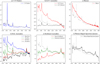 |
Fig. 9 Composite spectra for all anomaly categories identified in this project. In each plot, the gray dotted spectrum represents the Vanden Berk et al. (2001) composite. All mean spectra are aligned at the Mg II emission peak to ensure consistent comparison across categories. |
4.2.3 Group 3
For both datasets, Group 3 is shown in green scatter points located in the top-right region of the PCA 1 versus PCA 2 plot (see top panels of Fig. 8). The position is indicative of large coefficients for PCA 1 and 2 both translating to broad emission lines along with reddening continuum.
BAL dataset: This anomaly group is placed at the upper right section of the PCA 1 versus PCA 2 plot (see top panel of Fig. 8), indicating maximum values of PCA 1 and PCA 2 coefficients. These large values correspond to the strong reddening and broad line features observed in its members. Upon secondary grouping as described in Sect. 3.3, this group was divided into two parts: (1) red BALs and (2) FeLoBALs; the latter are a subset of LoBALs with absorption lines from iron transitions (excited-to-ground state), known as FeLoBALs. There are a total of 403 members in this group constituting 16.7% of the total anomalies.
Non-BAL dataset: Similar to the group 3 of the BAL dataset, this group is also present at the top right part of the PCA 1 versus PCA 2. Upon a secondary k-means clustering this group was divided into three parts: heavily reddened, moderately reddened, and plateau-shaped spectrum quasars. While the heavily reddened quasars have a steep positively sloping spectrum, the moderately reddened quasars have a relatively flat continuum. The third subgroup here, is a new type of quasar population, which we refer to as “plateau-shaped spectrum quasars”. Plateau-shaped spectrum quasars exhibit a spectral break around 2000 Å. Blueward of this break, their spectra display a flatter continuum, while redward of the break, the spectrum becomes steeper and bluer (see panel (f) in Fig. 9). These plateau-shaped spectrum quasars are present in the lowermost section of the group’s PCA spread (see black scatter points in the right panel of Fig. 12) due to their relatively bluer continua. Heavily reddened quasars constitute 60 percent of the total population of this group while the rest 40 percent is equally made of moderately reddened quasars and plateau-shaped spectrum quasars.
4.2.4 Group 4
Shown at the bottom-most region of the PCA 1 versus PCA 2 plot for both the datasets, group 4 members have the minimum values of PCA 2 coefficient and hence the bluest continuum. The members of this group are depicted by red scatter points in the top panels of Fig. 8.
BAL dataset: This group is depicted by the red scatter in the top-left panel of Fig. 8, located in the bottom-most region of the PCA distribution. Consequently, these quasars exhibit a steeply declining continuum toward longer wavelengths, along with prominent C IV and Si IV emission lines. We refer to these quasars as blue BALs: quasars with strong high-ionization absorption lines and a steep blue continuum. This is notable, as typical BAL quasars tend to exhibit significant reddening. This group has 122 members which accounts for ≈5% of the total anomalies.
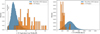
Fig. 10 Distribution of C IV EW and FWHM for all quasars in the Wu & Shen (2022) catalog (blue) compared to the C IV peakers (orange). The C IV EW for the C IV peakers is concentrated at the higher end of the distribution, while their FWHM is generally lower, indicating a strong yet narrow C IV emission line.
Non-BAL dataset: This group is depicted by the red scatter in the top-right panel of Fig. 8, located in the bottom-most region of the PCA distribution. Therefore, these quasars are characterized by a strongly downward-sloping continuum with equally strong C IV and Si IV emission lines. Hereafter, we call these quasars as Excess Si IV emitters. There are 227 Excess Si IV Emitters, representing 0.27% of the total quasars in our sample and approximately 11.3% of the total anomalies. This group also features the identification of 13 blazars, which lack any emission line but have a similar steep downward sloping spectrum as a typical Si IV Excess anomaly (refer to panel (c) in Fig. 9) for the mean spectrum of the 13 blazars). These blazars are present in the lower extreme of the Si IV excess anomalies spread in the PCA eigenspace in the top panel of Fig. 8.
5 Discussion
We have identified ten distinct groups of spectroscopic anomalies in the SDSS DR16 quasar catalog by applying hierarchical unsupervised k-means clustering to the spectral PCA decompositions. BAL quasars are well known for having spectra that differ from normal quasars due to the presence of strong absorption features. To prevent BAL quasars from being identified as major anomalous groups, we analyzed two disjoint datasets: one containing only BAL quasars, called the BAL dataset, and another devoid of BAL quasars, called the non-BAL dataset. This approach classified 81 780 quasars into three clusters, ensuring that quasars within each cluster have similar spectral characteristics, regardless of their luminosities.
The composite spectra of these clusters exhibit several properties that contribute to their unique separation. Cluster 1 (see top panel of Fig. 7) in both the datasets exhibits nearly identical spectrum as the striking, extremely strong C IV peak dilutes the impact of BAL signature absorption on the spectrum. The anomaly clusters in both datasets show a similar distribution and spread across all groups. The BAL QSOs in the BAL dataset result in more diffuse and broader spectral clusters, likely due to their strong absorption lines characteristics. In contrast, the absence of BAL QSOs in the non-BAL dataset produces more distinct and narrower spectral clusters, suggesting that BAL features contribute significantly to spectral variability, particularly at the bluer end of the UV-optical spectrum.
In this section, we analyze the distribution of the EWs, line ratios, and the full width at half maximum (FWHM) for prominent emission lines. These values are derived from the Wu & Shen (2022) catalog, which uses the PyQSOFit (Guo et al. 2018) software to calculate the parameters. This analysis is done across all anomaly groups to gain deeper insights into the underlying physics of each group. Inferences are drawn from the analyzed distributions and attributed to specific physical properties, as supported by findings from previous studies. A detailed characterization of each anomaly group, including multi-wavelength and multi-epoch analysis of individual objects, is outside the scope of this paper and will be explored in future studies.
5.1 C IV peakers
Members of this group are characterized by an exceptionally strong and narrow C IV emission line, accompanied by a weak, flat continuum (see panel a in Fig. 9). Fig. 10 shows the comparison of the C IV EW (left; a) and C IV FWHM (right; b) of the C IV peakers to that of all the quasars in the Wu & Shen (2022) catalog. For this group the median C IV FWHM is 2139 ± 170 km s−1, which is 0.53 times smaller than the median C IV FWHM of all the quasars in the Wu & Shen (2022) catalog. Additionally, the median FWHMs of all other emission lines (Si IV, He II, C III, Mg II) are also lower, ranging from 0.4 to 0.7 times their respective medians in the Wu & Shen (2022) catalog.
In terms of EWs, the median C IV EW is 173 ± 4 Å which is ~3.7 times the median C IV EW of all the quasars in Wu & Shen (2022). Except for the leftmost point in the Fig. 10b, which was identified as a Narrow Line Seyfert 1 (NLS1) galaxy as documented by Rakshit et al. (2021), the majority of the C IV peakers occupy the high EW end of the distribution. Despite the extremely high EWs, the C IV FWHM for these quasars remains on the lower end of the distribution, indicating that the extreme EW is driven by their exceptional line strength. However, five samples display relatively high FWHM alongside sharply peaked C IV emission (see Fig. 10b).
Additionally, along with C IV, the median EW of the He II line is about 2.33 times stronger than the median He II EW of all quasars in Wu & Shen (2022). However, the median EW values for Si IV, C III, and Mg II align closely with the median values observed in Wu & Shen (2022). The flux ratio, defined as the ratio of integrated fluxes between two lines, and the EW ratio of any line relative to C IV for this group are positioned at the extremely low end of the distribution compared to all quasars in Wu & Shen (2022), due to the exceptionally high strength of the C IV line. This suggests that the anomalous behavior is primarily driven by the extraordinary strength and EW of the C IV emission line. The C IV emission line stands out as the most prominent feature within the chosen wavelength window in our analysis for nearly all quasars (except for a few BALs), underscoring the algorithm’s effectiveness in identifying this strong line characteristic.
The C IV emission line, located at the higher end of the UV spectrum, predominantly originates from the accretion disk near the central black hole (Peterson 1997). It arises from the 2P3/2,1/2 → 2S1/2 (C+++ ground state) transition. As a major coolant for gas at high temperatures, well above 104 K (Ferland et al. 1996), the C IV emission is significantly enhanced. C IV λ1550 Å has an ionization potential of 64 eV, while He ir λ1640 Å has an ionization potential of 54 eV. Strong high-ionization lines like C IV and He II are typically indicative of a high ionization parameter, Γ ≥ 10−2 or harder continua (see Marziani et al. 1996).
A comprehensive explanation for the extremely high C IV flux and equivalent line width is provided by Fu et al. (2022) (hereafter F22), who conducted UV-Optical and X-ray analyses of eight quasars with very high C IV EW (>150 Å). Notably, two of these quasars are present in our group. In the F22 sample, large HeII EWs are also observed, indicating that the high-ionization BLR is receiving a significant number of ionizing photons, consistent with a hard ionizing continuum. F22 discusses the possibility that sources with large C IV EWs may represent the “opposite extreme” to weak line quasars (WLQs), which typically exhibit small C IV EWs, large C IV blueshifts, and weak X-ray emission. Overall, WLQs are often explained as quasars with high Eddington ratios, resulting in a geometrically and optically thick inner accretion disk that drives outflows. The thick inner disk together with the outflows can prevent ionizing EUV and X-ray photons from reaching the high-ionization broad emission line region and, in some cases, block the line of sight to the central X-ray-emitting region (e.g., Ni et al. 2018, 2022). In contrast, quasars with large C IV EWs may have relatively low Eddington ratios and minimal intrinsic absorption. Finally, F22 concluded that the enhancement in C IV and He II is best explained by the combined effects of a hard ionizing continuum and subsolar metallicity. Due to excessive C IV emission, the Si IV to C IV flux ratio is found to be 0.13 for these quasars, as compared to an average of 0.75 for all quasars in the Wu & Shen (2022) catalog. An enhanced high-ionization recombination line like He II suggests a harder ionizing continuum. In combination with this harder continuum, lower metallicity results in C IV becoming the dominant coolant. The strength of resonance lines depends on both ionic abundance and ionizing conditions. In a lower metallicity environment, other lines are not significantly enhanced due to reduced ionic abundance, whereas C IV remains prominent as the primary coolant under these conditions.
5.2 Excess Si IV emitters
These quasars are characterized by the presence of Si IV and C IV emission lines of nearly equal strength, accompanied by a strongly negative-sloped bluer continuum (see panel (b) in Fig. 9). A total of 227 such objects were identified in our study. The median Si IV EW of this group is 9.19 ± 0.46 Å, which is nearly equal to the median Si IV EW of all quasars in the Wu & Shen (2022) catalog. In contrast, the median EWs of other spectral lines in this group are reduced by approximately 40% to 50% compared to their respective median values in the Wu & Shen (2022) catalog. For this group, the EW ratio of Si IV to other lines – such as C IV, He II, C III, and Mg II – is approximately twice that of the corresponding EW ratios in the Wu & Shen (2022) catalog. This suggests that the overall anomalous nature of these quasars is primarily due to the heightened Si IV emission relative to other lines. The left panel of Fig. 11 shows the distribution of the flux ratio of Si IV to C IV emission lines for the excess Si IV emitter group compared to the distribution in the Wu & Shen (2022) catalog.
The median emission flux ratio of Si IV to C IV in the Wu & Shen (2022) catalog is approximately 0.72. However, for this group, the ratio increases to about 0.99, as indicated by the peak centered around 1 in the left panel of Fig. 11. This shift is attributed to a combination of factors: the Si IV emission flux is 4.2 times stronger, while the C IV flux is only half as strong. As a result, the Si IV and C IV emission line peaks reach nearly the same height, and in many cases, the Si IV peak even surpasses the C IV peak in this group’s spectra.
We note that the He II emission line in this group is significantly broader, with a FWHM nearly three times the median He II FWHM of all quasars in the Wu & Shen (2022) catalog. In contrast, the FWHM distributions for other lines (C IV, Si IV, C III, Mg II) closely match those of the quasars in the Wu & Shen (2022) catalog.
Nagao et al. (2006) demonstrated that the flux ratio of [Si IV + O IV] to C IV is a key diagnostic for probing the physical conditions and chemical composition of gas in quasars, particularly within the BLR, as the relative role of C IV as a coolant diminishes with increasing BLR metallicity. Our analysis reveals an Si IV /C IV flux ratio of approximately 1.4 (compared to an average of ≈0.75 for the overall dataset). According to Hamann et al. (2002), such a high ratio is indicative of super-solar BLR gas metallicities. This elevated metallicity reflects the presence of heavy elements produced in star-forming regions and incorporated into the quasar’s environment, a process often referred to as “chemical enrichment”. Consequently, the elevated Si IV/C IV ratio in this group suggests super-solar BLR gas metallicities, possibly due to unusual stellar activity near the galactic nuclei, which could explain their anomalous nature.
5.3 Si IV deficient anomalies
This group can be considered the counterpart to the Si IV Excess group discussed earlier. In these quasars, we observe reduced Si IV emission compared to Wu & Shen (2022) quasars, while the C IV emission between the two samples remains comparable. Their spectra typically exhibit a characteristic flatter continuum. Some members (~18%) also display notably enhanced iron emissions (~44–53%) between 2250 and 2700 Å. The ratio of Si IV to C IV flux for this group is 0.23, compared to 0.75 for the entire quasars in the Wu & Shen (2022) catalog. This ratio, which serves as a metallicity indicator for the BLR, points to an extremely low (subsolar) metallicity of Z/Z⊙ ≈ 0.4. This implies that the BLR metallicity for this group is nearly 40 times lower than that of the Si IV Excess quasars. Additionally, we also note that the median Mg II integrated flux shows a substantial increase of approximately 1.8 times compared to the median of Wu & Shen (2022) quasars.
The black dash-dot spectrum in the bottom right panel of Fig. 8 shows the mean spectra of the members of this group. It closely resembles the Flat BAL spectrum (see panel (d) in Fig. 9), which is predominantly composed of LoBAL quasar spectra. This resemblance arises because, in BAL quasars, the wide absorption troughs also result in a reduction of Si IV emission line flux, creating a similar spectral appearance.
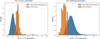 |
Fig. 11 Top: distribution of the ratio of Si IV to C IV emission line flux for the Excess Si IV emitters group (orange) compared to all quasars in the Wu & Shen (2022) catalog (blue). The Si IV to C IV ratio centered around 1 signifies an enhanced Si IV emission, where the Si IV emission line is as strong as the C IV line. Bottom: distribution of the ratio of Si IV to C IV emission line flux for the Si IV deficient group (orange) compared to all quasars in the Wu & Shen (2022) catalog (blue). |
Number of members in each BAL anomaly subgroup.
5.4 BAL anomalies
There are four types of BAL anomalies as discussed in Sect. 4.2. The majority of HiBAL quasars are not identified as anomalies because HiBAL QSOs, which constitute approximately 85% of the BAL population, are well captured by the PCA. The eigenvectors effectively adapt to map HiBAL features, ensuring that most typical HiBAL quasars are not marked as anomalies. As a result, the four BAL anomaly groups represent a minor subset of the BAL population, primarily due to the large number of HiBAL quasars that are included in the dataset. The total number of anomalies in each group is given in Table 4.
5.4.1 Blue BALs
We define blue BALs as BAL quasars with a significantly bluer continuum spectral index (α). These quasars exhibit strong C IV and Si IV absorption lines paired with a steep, downward-sloping spectrum resembling the Si IV excess anomalies, as seen in panel (d) and (b) in Fig. 9. They do not show any signs of reddening and have significantly higher emission flux towards the high-energy end of the spectrum, which rapidly decreases with increasing wavelength. This is unusual of a BAL quasar as most of them are known to be redder than a typical quasar (Menou et al. 2001). Due to the absence of reddening, they are positioned at the bottom part (with low PCA 2 coefficients) in the left panel of Fig. 12. The Mg II emission line is feeble or visibly absent in most of these quasars. This category of BAL anomalies is rare with only 103 such quasars detected in our analysis, with all of them being HiBAL quasars. Interestingly, the spectral shape of these blue BAL quasars coincide with the Vanden Berk et al. (2001) composite, with the only difference being the deep C IV and Si IV absorption troughs. This can be seen as an exception to the results by Reichard et al. (2003a) who found all HiBAL quasars in their study to be prominently redder than the SDSS Early Data Release (EDR) QSOs.
5.4.2 Flat BALs
The quasars in this group have a flat spectrum with nearly the same continuum flux throughout the wavelength range (i.e., nearly a zero power law). This feature is indicative of significant reddening which diminishes the flux at shorter wavelengths, making it comparable to the longer wavelength flux (see Hopkins et al. 2004). Their spectral slope is in between the blue BALs (steep downward slope) and reddened BALs (steep upward slope) which corresponds to their placement in the PCA eigenspace (the green scatter points in the left panel of Fig. 12).
About 80% of these flat BALs are LoBAL QSOs or Mg II BAL quasars. LoBALs are an important yet poorly understood class of quasars that provide direct evidence for energetic and variable mass outflows (e.g., see Vivek et al. 2014; Yi et al. 2019b,a). As noted by Wethers et al. (2019), LoBALs constitute about 15% of the total BAL quasar population, with HiBAL quasars making up the majority. As seen in panel d of Fig. 9, the composite Flat BAL spectrum (green) is significantly redder than both the blue BAL composite (blue) and the Vanden Berk et al. (2001) composite, consistent with the findings of Reichard et al. (2003a). This is the largest BAL anomaly group with a total of 371 members out of which 15 BALs are also cataloged by Trump et al. (2006).
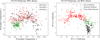 |
Fig. 12 Left: 2D projection of G2+G3 BAL anomalies (using PCA 1 versus PCA 2 coefficients) as grouped into three types by the secondary k-means clustering as discussed in Sect. 3.3. The reddened and FeLoBALs are placed on the upper region with higher PCA 2 coefficients pertaining to largely amount of reddening in their spectra. Flat BALs, usually with a flat spectrum are placed in the middle left region. Right: 2D projection of reddened anomalies (using PCA 1 versus PCA two coefficients) as grouped into three subtypes by the secondary k-means clustering as discussed in Sect. 3.3. The heavily reddened quasars, characterized by steeply sloped spectra, are positioned in the upper region with higher PCA 2 coefficients. Moderately reddened quasars, exhibiting a flat continuum, occupy the middle region. Quasars with plateau-shaped spectra are located in the lower region of the distribution, with the lowest PCA 2 coefficients, due to their overall negative slope. |
5.4.3 Red BALs
These quasars exhibit a strongly positively sloped spectrum with a redder continuum spectral index, indicating significant dust reddening (see red spectrum in panel d of Fig. 9). This reddening corresponds to significantly higher PCA 2 coefficients. The members of this group are characterized by broad C IV absorption lines that strongly suppress the blue part of the emission line, along with prominent iron absorption features in most cases. The group comprises 276 objects, of which 60% are FeLoBALs and the remaining 40% are LoBAL quasars.
The FeLoBAL quasars in this group differ from classical FeLoBALs (another subgroup within BAL anomalies) primarily due to their narrower iron absorption lines. Because of this distinction (and the occasional ambiguity in identifying Fe II absorption due to strong reddening and low Fe II strength) we opted not to combine these FeLoBALs with the classical FeLoBALs.
Notably, these BAL quasars are significantly redder than the composite LoBAL spectra constructed by Reichard et al. (2003b). Consistently, members of this group exhibit even stronger reddening than the Flat BAL group (which predominantly consists of LoBALs). This trend is consistent with findings by Hamann et al. (2017), who confirmed that BAL quasars are more frequently associated with redder quasars and tend to have stronger or deeper absorption profiles.
5.4.4 FeLoBALs
The rare class of LoBAL quasars with absorptions from metastable excited states of Fe II are known as FeLoBAL quasars (Becker et al. 2000; Choi et al. 2022). This group consists exclusively of extreme cases of these BAL quasars. Typical members exhibit properties such as absorptions from over 20 transitions involving at least a dozen elements, similar to SDSS 1723+5553, as analyzed by Hall et al. (2002). The broad-band spectral properties of FeLoBALs are thought to indicate scenarios such as mergers, star burst, etc. (e.g., Farrah et al. 2010). In addition, “Unusual” FeLoBALs can also be indicative of unique mechanisms such as a resonance-scattering interpretation of FeLoBAL 1214+2803 by Branch et al. (2002).
The composite spectrum of the 121 members of this group is shown in panel d of Fig. 9. Most members feature extremely broad and deep absorption lines that significantly obscure the continuum, resulting in a highly unusual spectrum. In the PCA eigenspace, these quasars occupy a region similar to that of the reddened BALs, as FeLoBALs represent some of the most extreme cases of reddening observed in BAL quasars.
5.5 Reddened anomalies
Reddened quasars are a subset of AGNs whose spectra exhibit significant attenuation at shorter wavelengths due to the presence of dust. This dust absorbs high-energy ultraviolet and blue light, re-emitting it at longer, redder wavelengths, producing a characteristic “reddening” effect. These quasars provide unique insights into the interplay between quasar activity and the surrounding interstellar medium, as well as the dust content within the host galaxy (see Shao et al. 2022). Reddened quasars are often associated with high levels of star formation and dust-rich environments, which may obscure the central black hole and impact the observed properties of the quasar (e.g., Andonie et al. 2022). As discussed by Hopkins et al. (2004), there could be several other processes too that result in a redder spectrum such as an intrinsically red continuum, an excess of synchrotron emission in red, intervening absorption by galaxies along the line of sight, or dust extinction in the host galaxy or the quasar central engine itself. In our analysis, we identified three groups of reddened anomalies, which are discussed below.
Sample table listing the anomalous quasars identified in this work.
5.5.1 Heavily reddened quasars
This group consists of 165 quasars exhibiting a spectrum with excessive positively sloped continuum (see panel e in Fig. 9); namely, they are significantly redder continuum spectral index. Due to the reddening, they are represented by high values of PCA 2 coefficient placing them in the topmost region of the PCA eigenspace as shown by red scatter points in the right panel of Fig. 12. Nearly all members of this group closely resemble the “too red” composite seen in (Fig. 7 Richards et al. 2003), indicating that this group represents the extreme cases of reddening in quasars. Additionally, some members also feature narrow absorption lines. Hopkins et al. (2004) showed that reddened quasars are much more likely to show narrow absorption at the redshift of the quasar than are unreddened quasars.
5.5.2 Moderately reddened quasars
This group refers to quasars with a rather constant flux throughout the wavelength range. Visual inspection revealed that this group actually consists of two subgroups: one with a flat continuum and another with a convex-shaped continuum (see green plot in panel e of Fig. 9). The reddening in this group is less pronounced compared to heavily reddened quasars. The mean spectrum of this group traces the “dust reddened” composite of (Richards et al. 2003, Fig. 7), which features a zero power law continuum between the rest wavelength of 1300 Å and 3000 Å. They are placed aptly below the heavily reddened quasars in the right panel of Fig. 12, with smaller PCA 2 coefficients representing the lesser extent of reddening. The Mg II emission in the members of this group is nearly identical to that of the heavily reddened quasars. This group also contains peculiar cases of quasars with a spectrum resembling an inverted parabola. We call these quasars as “convex” members. The inverted-parabola spectrum of these convex members has a peak luminosity around 2000 Å which tapers off symmetrically toward both ends. Some members also display narrow absorption lines, particularly toward the redder part of the spectrum. The spectra of these convex members is identical to that of the plateau-shaped spectrum (see Sect. 5.6) quasars between 2000 and 3000 Å. However, between 1250 and 2000 Å, where the plateau-shaped spectrum quasars show a constant flux, convex members show a sharp positively sloped continuum. In terms of visual appearance, the convex quasars are closer to the plateau-shaped spectrum quasars, but are placed with the moderately reddened quasars instead. This is because, in the PCA projection (see the right panel of Fig. 12) the convex members are placed along with the moderately reddened quasars (in the green group) whereas, the plateau-shaped spectrum quasars are spatially separated and clustered distinctively. There are a total of 93 quasars belonging to this group.
5.6 Plateau-shaped spectrum quasars
The continuum of these quasars can be characterized into two segments. The first half (1250–2000 Å) exhibits a relatively flat continuum with broad Si IV and C IV emission lines. The second half (2000–3000 Å) rapidly falls with increasing wavelength. These quasars are termed as “plateau-shaped spectrum” quasars. This is because the flat (or slightly convex) feature together with the steeply sloped latter half of the spectrum imparts a plateau appearance to the continuum (see panel f in Fig. 9). The members of this group have a nearly equally strong C IV and Si IV emission peak, which is caused by substantially less C IV emission flux as compared to a typical quasar. The He II strength as well as the flux between 1640 Å and 1910 Å in these quasars is significantly more than that of a typical quasar. These quasars also show a strong Mg II emission line along with an enhanced iron emissions between 2250 and 2750 Å.
5.7 Machine error anomalies
All the anomaly groups also consistently include anomalies caused by corrupted spectra. These anomalies often feature extended regions of distortions or interpolation with a line connecting the disjoint sections. One of the most consistent anomalies is the quasars featuring a sharp narrow Dirac-Delta function-like peak caused by a cosmic ray encounter as discussed in Sect. 5.1. These were removed from the C IV peakers group by a simple threshold cut on the C IV line’s EW. Other occasional machine error anomalies were visually identified and discarded, as they do not contribute to any meaningful scientific analysis.
The full list of anomalous quasars identified in this work is available as a value-added catalog with this paper. Table 5 provides a sample list, including the quasar name, right ascension, declination, and redshift, along with the cluster group numbers and their final anomaly classification.
6 Conclusion
Applying hierarchical k-means clustering in a 20-dimensional PCA eigenvector hyperspace representing quasar spectra. We have presented five broad categories of quasar anomalies divided into 10 homogeneous groups:
C IV peakers: A total of 299 quasars with an extremely strong, yet narrow (median ~2000 km s−1) C IV emission line;
Excess Si IV emitters: Quasars in this group exhibit an excessively high Si IV to C IV emission line flux ratio, nearly double the median value observed for all quasars in Wu & Shen (2022) catalog. A total of 227 such quasars were found;
Si IV deficient anomalies: 328 quasars with disproportionately low Si IV emission with Si IV to C IV flux ratio being one third of the median ratio for all quasars in Wu & Shen (2022) catalog;
BAL anomalies: A total of 871 quasars were identified as anomalies with BAL profiles. These were further subdivided into four subgroups as follows:
Blue BALs: A total of 103 HiBAL quasars with a strong negatively sloped (“blue”) continuum which is atypical of a BAL quasar;
Flat BALs: 371 BAL quasars with a relatively flat continuum. Among these, 80% are LoBAL quasars;
Reddened BALs: A total of 276 BAL quasars with heavily reddened continuum, hence, with a strongly positive slope spectra;
FeLoBALs: These are a very rare class of BAL quasars with strong Fe absorptions and heavily reddened continua. There are a total of 121 such quasars detected.
Reddened anomalies: A total of 341 quasars were identified as reddened anomalous quasars, characterized by extreme reddening, as evident from their significantly red spectral slope. They were further subdivided into three subgroups primarily based on the degree of reddening, as follows:
Heavily reddened quasars: A total of 165 quasars were identified with steep, positively sloped spectra, attributed to heavy dust reddening;
Moderately reddened quasars: Dust reddened quasars with relatively flat or slightly convex shaped continuum. A total of 93 such quasars were found;
Plateu-shaped spectrum quasars: A total of 83 peculiar quasars were identified with a plateau-shaped spectrum, characterized by a flat continuum followed by a negatively sloped continuum. These quasars exhibit a nearly flat continuum between 1250 and 2000 Å, which then rapidly declines as the wavelength increases from 2000 to 3000 Å.
In our analysis, we initially applied the methodology to the entire dataset without distinguishing BAL quasars from non-BAL quasars. This approach aimed to demonstrate what one would obtain if all spectra were analyzed without prior classifications; that is, working with spectral data as they are obtained by the spectroscopic surveys. However, this resulted in groups that were not as pure, making interpretation more challenging. Ultimately, we found that preclassifying BAL quasars significantly simplified the process and led to much cleaner and more distinct groupings. This highlights the importance of BAL classification as a preliminary step when working with large spectroscopic datasets. We recommend that future studies employing similar techniques first isolate BAL quasars before applying clustering or statistical analyses to ensure clearer and more meaningful results.
This work has significantly expanded the number of sources in each anomalous quasar group. For example, we present a sample of 121 extreme FeLoBALs with strong, broad Fe II absorption, along with an additional 127 FeLoBALs from the red BAL anomalies, where the iron absorption lines are considerably narrower. We have developed an efficient method for identifying anomalous quasars and classifying them into distinct categories. The detected anomalies are presented in a value-added catalog, available at the SQuAD website1. This approach has been successfully applied to the rest-frame UV spectra from the SDSS DR16 catalog and is currently being prepared for broader implementation. We applied the same algorithm to rest-frame optical spectra from SDSS DR16, covering around 75 000 quasars in the redshift range 0.1 ≤ z ≤ 1.1, including key emission lines such as O III, Hβ, and optical iron. This catalog will be crucial, as these emission lines, particularly in the context of Eigenvector 1, are tightly correlated with the accretion rate and orientation of quasars (see Shen & Ho 2014). The catalog is currently under preparation.
With upcoming large-scale surveys such as Dark Energy Spectroscopic Instrument (DESI), 4-metre Multi-Object Spectroscopic Telescope (4MOST), and William Herschel Telescope (WHT) Enhanced Area Velocity Explorer (WEAVE), the number of quasar spectra will increase significantly, and our methodology will aid in identifying anomalous quasars in these vast datasets. Additionally, our approach can be adapted for photometric surveys, such as the Legacy Survey of Space and Time (LSST) survey, to find photometrically anomalous quasars. By extending the sample size of these anomalous quasars, this study enables the statistical analysis of these peculiar sources, contributing to a deeper understanding of AGNs and their diverse characteristics.
Data availability
Table 5 is available at the CDS via anonymous ftp to cdsarc.cds.unistra.fr (130.79.128.5) or via https://cdsarc.cds.unistra.fr/viz-bin/cat/J/A+A/699/A132
Acknowledgements
We thank the anonymous referee for the feedback which has significantly helped to improve the paper. AT acknowledges and thanks the Indian Institute of Astrophysics (IIA) for their acceptance in the visiting student program (VSP) and hence the financial and infrastructural support provided. MV acknowledges support from Department of Science and Technology, India – Science and Engineering Research Board (DST-SERB) in the form of a core research grant (CRG/2022/007884). Funding for the Sloan Digital Sky Survey IV has been provided by the Alfred P. Sloan Foundation, the U.S. Department of Energy Office of Science, and the Participating Institutions. SDSS acknowledges support and resources from the Center for High-Performance Computing at the University of Utah. The SDSS web site is https://www.sdss4.org. SDSS is managed by the Astrophysical Research Consortium for the Participating Institutions of the SDSS Collaboration including the Brazilian Participation Group, the Carnegie Institution for Science, Carnegie Mellon University, Center for Astrophysics I Harvard & Smithsonian (CfA), the Chilean Participation Group, the French Participation Group, Instituto de Astrofísica de Canarias, The Johns Hopkins University, Kavli Institute for the Physics and Mathematics of the Universe (IPMU)/University of Tokyo, the Korean Participation Group, Lawrence Berkeley National Laboratory, Leibniz Institut für Astrophysik Potsdam (AIP), Max-Planck-Institut für Astronomie (MPIA Heidelberg), Max-Planck-Institut für Astrophysik (MPA Garching), Max-Planck-Institut für Extraterrestrische Physik (MPE), National Astronomical Observatories of China, New Mexico State University, New York University, University of Notre Dame, Observatório Nacional / MCTI, The Ohio State University, Pennsylvania State University, Shanghai Astronomical Observatory, United Kingdom Participation Group, Universidad Nacional Autónoma de México, University of Arizona, University of Colorado Boulder, University of Oxford, University of Portsmouth, University of Utah, University of Virginia, University of Washington, University of Wisconsin, Vanderbilt University, and Yale University.
Appendix A SQuAD algorithm
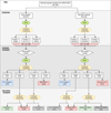 |
Fig. A.1 Flowchart showing the steps followed by our algorithm, beginning from the quasar sample selection to the final anomaly groups obtained. |
Appendix B PCA eigenvectors
The PCA Eigenvectors for the primary k-means clustering are given in Fig. B.1.
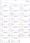 |
Fig. B.1 Each of the 20 components of the PCA decomposition shown in each panel (red dashed line for BAL dataset; blue solid line for non-BAL dataset). Each component represents an eigenvector of the 20 component PCA. The first plot on the top depicts the mean spectrum of the total dataset. This mean spectrum is coincident with the Vanden Berk et al. (2001) composite spectrum which reinforces the generalized nature of our selected data sample. |
References
- Andonie, C., Alexander, D. M., Rosario, D., et al. 2022, MNRAS, 517, 2577 [NASA ADS] [CrossRef] [Google Scholar]
- Artymowicz, P. 1993, PASP, 105, 1032 [NASA ADS] [CrossRef] [Google Scholar]
- Becker, R. H., White, R. L., Gregg, M. D., et al. 2000, ApJ, 538, 72 [NASA ADS] [CrossRef] [Google Scholar]
- Begelman, M. C., Blandford, R. D., & Rees, M. J. 1984, Rev. Mod. Phys., 56, 255 [Google Scholar]
- Boroson, T. A., & Green, R. F. 1992, ApJS, 80, 109 [Google Scholar]
- Bozdogan, H. 1987, Psychometrika, 52, 345 [CrossRef] [MathSciNet] [Google Scholar]
- Bradley, P. S., & Fayyad, U. M. 1998, in ICML [Google Scholar]
- Branch, D., Leighly, K. M., Thomas, R., & Baron, E. 2002, ApJ, 578, L37 [NASA ADS] [CrossRef] [Google Scholar]
- Brotherton, M., Tran, H. D., Becker, R., et al. 2001, ApJ, 546, 775 [NASA ADS] [CrossRef] [Google Scholar]
- Carnall, A. C. 2017, SpectRes: A Fast Spectral Resampling Tool in Python [Google Scholar]
- Choi, H., Leighly, K. M., Terndrup, D. M., et al. 2022, ApJ, 937, 74 [NASA ADS] [CrossRef] [Google Scholar]
- Collin, S., Boisson, C., Mouchet, M., et al. 2002, A&A, 388, 771 [NASA ADS] [CrossRef] [EDP Sciences] [Google Scholar]
- Cousineau, D., Brown, S., & Heathcote, A. 2004, BRM-IC, 36, 742 [Google Scholar]
- Diamond-Stanic, A. M., Fan, X., Brandt, W., et al. 2009, ApJ, 699, 782 [NASA ADS] [CrossRef] [Google Scholar]
- Farrah, D., Urrutia, T., Lacy, M., et al. 2010, ApJ, 717, 868 [NASA ADS] [CrossRef] [Google Scholar]
- Ferland, G. J., Baldwin, J. A., Korista, K. T., et al. 1996, ApJ, 461, 683 [NASA ADS] [CrossRef] [Google Scholar]
- Francis, P. J., Hewett, P. C., Foltz, C. B., & Chaffee, F. H. 1992, AJ, 398, 476 [Google Scholar]
- Fu, S., Brandt, W., Zou, F., et al. 2022, ApJ, 934, 97 [NASA ADS] [CrossRef] [Google Scholar]
- Green, P. J., Pulgarin-Duque, L., Anderson, S. F., et al. 2022, ApJ, 933, 180 [NASA ADS] [CrossRef] [Google Scholar]
- Gregg, M. D., Lacy, M., White, R. L., et al. 2002, ApJ, 564, 133 [Google Scholar]
- Guo, Z., & Martini, P. 2019, ApJ, 879, 72 [Google Scholar]
- Guo, H., Shen, Y., & Wang, S. 2018, PyQSOFit: Python code to fit the spectrum of quasars, Astrophysics Source Code Library [record ascl:1809.008] [Google Scholar]
- Haardt, F., & Maraschi, L. 1991, ApJ, 380, L51 [Google Scholar]
- Hall, P. B., Anderson, S. F., Strauss, M. A., et al. 2002, ApJS, 141, 267 [NASA ADS] [CrossRef] [Google Scholar]
- Hamann, F., Korista, K., Ferland, G. J., Warner, C., & Baldwin, J. 2002, ApJ, 564, 592 [NASA ADS] [CrossRef] [Google Scholar]
- Hamann, F., Zakamska, N. L., Ross, N., et al. 2017, MNRAS, 464, 3431 [Google Scholar]
- Harris, D. W., Jensen, T. W., Suzuki, N., et al. 2016, AJ, 151, 155 [NASA ADS] [CrossRef] [Google Scholar]
- Henrion, M., Hand, D. J., Gandy, A., & Mortlock, D. J. 2013, Statist. Anal. Data Mining, 6, 53 [Google Scholar]
- Hines, D. C., Schmidt, G. D., Gordon, K. D., et al. 2001, ApJ, 563, 512 [Google Scholar]
- Hopkins, P. F., Strauss, M. A., Hall, P. B., et al. 2004, AJ, 128, 1112 [Google Scholar]
- Hubert, M., & Van der Veeken, S. 2008, J. Chemom., 22, 235 [Google Scholar]
- Koratkar, A., & Blaes, O. 1999, PASP, 111, 1 [Google Scholar]
- LaMassa, S. M., Cales, S., Moran, E. C., et al. 2015, ApJ, 800, 144 [NASA ADS] [CrossRef] [Google Scholar]
- Liu, Z., et al. 2011, Procedia Environ. Sci., 11, 256 [Google Scholar]
- Lyke, B. W., Higley, A. N., McLane, J. N., et al. 2020, ApJS, 250, 8 [NASA ADS] [CrossRef] [Google Scholar]
- Ma, B., Shang, Z., & Brotherton, M. S. 2019, RAA, 19, 169 [Google Scholar]
- Marziani, P., Sulentic, J., Dultzin-Hacyan, D., Calvani, M., & Moles, M. 1996, ApJ, 104, 37 [Google Scholar]
- Menou, K., Berk, D. E. V., Ivezić, Ž., et al. 2001, ApJ, 561, 645 [NASA ADS] [CrossRef] [Google Scholar]
- Meusinger, H., Schalldach, P., Scholz, R.-D., et al. 2012, A&A, 541, A77 [NASA ADS] [CrossRef] [EDP Sciences] [Google Scholar]
- Nagao, T., Marconi, A., & Maiolino, R. 2006, A&A, 447, 157 [NASA ADS] [CrossRef] [EDP Sciences] [Google Scholar]
- Napoleon, D., & Pavalakodi, S. 2011, IJCA, 13, 41 [Google Scholar]
- Newman, P. R., Long, D. C., Snedden, S. A., et al. 2004, in Ground-based Instrumentation for Astronomy, 5492, SPIE, 533 [Google Scholar]
- Ni, Q., Brandt, W., Luo, B., et al. 2018, MNRAS, 480, 5184 [NASA ADS] [Google Scholar]
- Ni, Q., Brandt, W., Luo, B., et al. 2022, MNRAS, 511, 5251 [NASA ADS] [CrossRef] [Google Scholar]
- Pâris, I., Petitjean, P., Rollinde, E., et al. 2011, A&A, 530, A50 [NASA ADS] [CrossRef] [EDP Sciences] [Google Scholar]
- Peterson, B. M. 1997, Taxonomy of Active Galactic Nuclei (Cambridge University Press), 21 [Google Scholar]
- Plotkin, R. M., Anderson, S. F., Hall, P. B., et al. 2008, AJ, 135, 2453 [NASA ADS] [CrossRef] [Google Scholar]
- Rakshit, S., Stalin, C., Kotilainen, J., & Shin, J. 2021, ApJS, 253, 28 [NASA ADS] [CrossRef] [Google Scholar]
- Razali, N. M., Wah, Y. B., et al. 2011, JOSMA, 2, 21 [Google Scholar]
- Reichard, T. A., Richards, G. T., Hall, P. B., et al. 2003a, AJ, 126, 2594 [NASA ADS] [CrossRef] [Google Scholar]
- Reichard, T. A., Richards, G. T., Schneider, D. P., et al. 2003b, AJ, 125, 1711 [NASA ADS] [CrossRef] [Google Scholar]
- Reis, I., Rotman, M., Poznanski, D., Prochaska, J., & Wolf, L. 2021, Astron. Comput., 34, 100437 [NASA ADS] [CrossRef] [Google Scholar]
- Richards, G. T., Hall, P. B., Berk, D. E. V., et al. 2003, AJ, 126, 1131 [Google Scholar]
- Sánchez Almeida, J., Aguerri, J. A. L., Muñoz-Tuñón, C., & de Vicente, A. 2010, ApJ, 714, 487 [Google Scholar]
- Satopaa, V., Albrecht, J., Irwin, D., & Raghavan, B. 2011, in 2011 31st ICDCS Workshops, IEEE, 166 [Google Scholar]
- Savitzky, A., & Golay, M. J. E. 1964, Analyt. Chem., 36, 1627 [NASA ADS] [CrossRef] [Google Scholar]
- Schwertman, N. C., Owens, M. A., & Adnan, R. 2004, CSDA, 47, 165 [Google Scholar]
- Seo, S. 2006, PhD thesis, University of Pittsburgh [Google Scholar]
- Shakura, N. I., & Sunyaev, R. A. 1973, A&A, 24, 337 [NASA ADS] [Google Scholar]
- Shao, Y., Wang, R., Weiss, A., et al. 2022, A&A, 668, A121 [NASA ADS] [CrossRef] [EDP Sciences] [Google Scholar]
- Shen, Y., & Ho, L. C. 2014, Nature, 513, 210 [NASA ADS] [CrossRef] [Google Scholar]
- Smee, S. A., Gunn, J. E., Uomoto, A., et al. 2013, AJ, 146, 32 [Google Scholar]
- Solarz, A., Thomas, R., Montenegro-Montes, F. M., et al. 2020, A&A, 642, A103 [NASA ADS] [CrossRef] [EDP Sciences] [Google Scholar]
- Suzuki, N. 2006, ApJS, 163, 110 [Google Scholar]
- Syakur, M., Khotimah, B. K., Rochman, E., & Satoto, B. D. 2018, in IOP Conference Series: Materials Science and Engineering, 336 (IOP Publishing), 012017 [Google Scholar]
- Trump, J. R., Hall, P. B., Reichard, T. A., et al. 2006, ApJS, 165, 1 [Google Scholar]
- Vanden Berk, D. E., Richards, G. T., Bauer, A., et al. 2001, AJ, 122, 549 [Google Scholar]
- Vivek, M., Srianand, R., Mahabal, A., & Kuriakose, V. C. 2012a, MNRAS, 421, L107 [Google Scholar]
- Vivek, M., Srianand, R., Petitjean, P., et al. 2012b, MNRAS, 423, 2879 [Google Scholar]
- Vivek, M., Srianand, R., Petitjean, P., et al. 2014, MNRAS, 440, 799 [Google Scholar]
- Wethers, C., Kotilainen, J., Schramm, M., & Schulze, A. 2019, Proc. IAU, 15, 285 [Google Scholar]
- Wiklind, T., & Combes, F. 1996, Nature, 379, 139 [Google Scholar]
- Wilhite, B. C., Vanden Berk, D. E., Kron, R. G., et al. 2005, ApJ, 633, 638 [Google Scholar]
- Wu, Q., & Shen, Y. 2022, ApJS, 263, 42 [NASA ADS] [CrossRef] [Google Scholar]
- Xiong, L., Poczos, B., Connolly, A., & Schneider, J. 2018, Anomaly Detection for Astronomical Data, Carnegie Mellon University, https://doi.org/10.1184/R1/6475475.v1 [Google Scholar]
- Yi, W., Brandt, W., Hall, P., et al. 2019a, VizieR Online Data Catalog: J/ApJS/242/28 [Google Scholar]
- Yi, W., Brandt, W., Hall, P., et al. 2019b, ApJS, 242, 28 [NASA ADS] [CrossRef] [Google Scholar]
- Yip, C.-W., Connolly, A., Berk, D. V., et al. 2004, AJ, 128, 2603 [Google Scholar]
- Zheng, W., Kriss, G. A., Telfer, R. C., Grimes, J. P., & Davidsen, A. F. 1997, ApJ, 475, 469 [NASA ADS] [CrossRef] [Google Scholar]
All Tables
All Figures
|
Fig. 1 Redshift distribution of quasars in the SDSS DR16 catalog (blue) and the selected subset of quasars (yellow) within the specified redshift range, 1.88 ≤ z ≤ 2.47. The red dashed curve represents the comoving distance, while the green dotted curve shows the lookback time as a function of redshift. The corresponding distance and time values at two key redshifts: z = 1.88 and z = 2.47, are marked. |
| In the text | |
|
Fig. 2 Example quasar spectrum showing the max-normalized flux before (blue) and after preprocessing (black). Note: the preprocessing effectively reduces noise without altering the overall spectral shape. |
| In the text | |
|
Fig. 3 Cumulative variance as a function of the PCA components for the PCA decomposition with 20 components, for both the BAL (red) and non-BAL (green) datasets. In both cases, a total explained variance of 94.9% is achieved with 20 PCA components. |
| In the text | |
|
Fig. 4 Sum of squared errors (SSE) and silhouette coefficients as a function of cluster numbers for the BAL (left) and non-BAL (right) datasets. The optimal number of clusters is determined using both the elbow (knee) method and the silhouette coefficient for both datasets. The knee of the SSE curve occurs at three for both datasets. |
| In the text | |
|
Fig. 5 Histograms show the distribution of the Euclidean distance of each point from its respective cluster centroid for the BAL (top panel) and non-BAL (bottom panel) datasets respectively. The red shaded region marks the respective threshold limits (Q3 + 1.5 × IQR; see Sect. 3.1). Quasars falling within the shaded region are identified as anomalous quasars. |
| In the text | |
|
Fig. 6 Sum of squared errors (SSE) and silhouette coefficients as a function of cluster numbers for the k-means clustering of anomalous quasars in the BAL and non-BAL datasets. The knee of the SSE curve occurs at four for both datasets, which coincides with the maxima of the silhouette coefficient. |
| In the text | |
|
Fig. 7 Top: 2D projection (PCA 1 versus PCA 2 coefficients) of the BAL (left) and non-BAL (right) datasets. Each dataset is divided into three clusters (cluster 1: brown, cluster 2: green, cluster 3: blue) within the 20-dimensional PCA hyperspace, using k-means clustering. Quasars classified as anomalous after applying a Q3 + 1.5 × IQR threshold are shown as black scatter points overlayed on top of the cluster members. The cluster centroids are marked by yellow crosses. Bottom: mean composite spectrum for each cluster of the BAL (left) and non-BAL (right) datasets. The color of each spectrum corresponds to the color of the cluster as shown in the top panel. The inset plot shows the mean cluster spectra normalized at λ = 2797 Å with the Vanden Berk et al. (2001) composite. The number of anomalies present in each cluster is given in Table 2. |
| In the text | |
|
Fig. 8 Top: 2D projection (PCA 1 versus PCA 2 coefficients) of the anomalies of the two datasets as divided into four groups each (group 1: blue, group 2: black, group 3: green, group 4: red) in the 20 dimensional PCA hyperspace, by the second k-means clustering applied only on the anomalous quasars. The groups as characterized by further analysis (see Sect. 5) are circled and labelled to reflect the nature of their anomaly. Bottom: mean composite spectrum of each anomaly group for both the datasets. The colors of the spectra correspond to the color of the corresponding group in the top panel. |
| In the text | |
|
Fig. 9 Composite spectra for all anomaly categories identified in this project. In each plot, the gray dotted spectrum represents the Vanden Berk et al. (2001) composite. All mean spectra are aligned at the Mg II emission peak to ensure consistent comparison across categories. |
| In the text | |
|
Fig. 10 Distribution of C IV EW and FWHM for all quasars in the Wu & Shen (2022) catalog (blue) compared to the C IV peakers (orange). The C IV EW for the C IV peakers is concentrated at the higher end of the distribution, while their FWHM is generally lower, indicating a strong yet narrow C IV emission line. |
| In the text | |
|
Fig. 11 Top: distribution of the ratio of Si IV to C IV emission line flux for the Excess Si IV emitters group (orange) compared to all quasars in the Wu & Shen (2022) catalog (blue). The Si IV to C IV ratio centered around 1 signifies an enhanced Si IV emission, where the Si IV emission line is as strong as the C IV line. Bottom: distribution of the ratio of Si IV to C IV emission line flux for the Si IV deficient group (orange) compared to all quasars in the Wu & Shen (2022) catalog (blue). |
| In the text | |
|
Fig. 12 Left: 2D projection of G2+G3 BAL anomalies (using PCA 1 versus PCA 2 coefficients) as grouped into three types by the secondary k-means clustering as discussed in Sect. 3.3. The reddened and FeLoBALs are placed on the upper region with higher PCA 2 coefficients pertaining to largely amount of reddening in their spectra. Flat BALs, usually with a flat spectrum are placed in the middle left region. Right: 2D projection of reddened anomalies (using PCA 1 versus PCA two coefficients) as grouped into three subtypes by the secondary k-means clustering as discussed in Sect. 3.3. The heavily reddened quasars, characterized by steeply sloped spectra, are positioned in the upper region with higher PCA 2 coefficients. Moderately reddened quasars, exhibiting a flat continuum, occupy the middle region. Quasars with plateau-shaped spectra are located in the lower region of the distribution, with the lowest PCA 2 coefficients, due to their overall negative slope. |
| In the text | |
|
Fig. A.1 Flowchart showing the steps followed by our algorithm, beginning from the quasar sample selection to the final anomaly groups obtained. |
| In the text | |
|
Fig. B.1 Each of the 20 components of the PCA decomposition shown in each panel (red dashed line for BAL dataset; blue solid line for non-BAL dataset). Each component represents an eigenvector of the 20 component PCA. The first plot on the top depicts the mean spectrum of the total dataset. This mean spectrum is coincident with the Vanden Berk et al. (2001) composite spectrum which reinforces the generalized nature of our selected data sample. |
| In the text | |
Current usage metrics show cumulative count of Article Views (full-text article views including HTML views, PDF and ePub downloads, according to the available data) and Abstracts Views on Vision4Press platform.
Data correspond to usage on the plateform after 2015. The current usage metrics is available 48-96 hours after online publication and is updated daily on week days.
Initial download of the metrics may take a while.