| Issue |
A&A
Volume 699, July 2025
|
|
|---|---|---|
| Article Number | A380 | |
| Number of page(s) | 13 | |
| Section | Extragalactic astronomy | |
| DOI | https://doi.org/10.1051/0004-6361/202452226 | |
| Published online | 25 July 2025 | |
Mocking integral field unit observations and metallicity diagnostics from cosmological simulations
1
Institute of Astronomy, Pontificia Universidad Católica de Chile, Av. Vicuña Mackenna 4860, Santiago 7820436, Chile
2
Research School of Astronomy and Astrophysics, Australian National University, Canberra, ACT, Australia
3
Nucleus Millenium ERIS, Santiago, Chile
4
Université Côte d’Azur, Observatoire de la Côte d’Azur, CNRS, Laboratoire Lagrange, F-06000 Nice, France
5
Instituto de Astrofísica de Andalucia, Glorieta de la Astronomía s/n, 18008 Granada, Spain
6
Instituto de Radioastronomía y Astrofísica (IRYA), UNAM, Campus, Morelia, Michoacán, C.P. 58089, México
7
Instituto de Estudios Astrofísicos, Facultad de Ingeniería y Ciencias, Universidad Diego Portales, Santiago de Chile, Chile
⋆ Corresponding author: This email address is being protected from spambots. You need JavaScript enabled to view it.
Received:
12
September
2024
Accepted:
27
May
2025
Abstract
Context. Hydrodynamic simulations are powerful tools for studying galaxy formation. However, it is crucial to test and improve the subgrid physics underlying these simulations by comparing their predictions with observations. To this aim, observable quantities can be derived for simulated galaxies, enabling the analysis of simulated properties through an observational approach.
Aims. Our goal is to develop a new numerical tool capable of generating synthetic emission line spectra from spatially resolved regions in simulated galaxies, carrying out mock integral field unit (IFU) observations.
Methods. We produced synthetic spectra of simulated galaxies by integrating the software CIGALE with the outcomes of hydrodynamical simulations. We considered the contributions from both stellar populations and nebular emission. The nebular emission lines in the spectra were modeled by considering only the contributions from the simulated star-forming regions. Furthermore, our model considers the properties of the surrounding interstellar medium to estimate the ionizing parameters, the metallicity, the velocity dispersion, and the electron density.
Results. We present the new numerical tool PRISMA. Leveraging synthetic spectra generated by our model, PRISMA successfully computed and recovered the intrinsic values of the star formation rate and gas-phase metallicity in local regions of simulated galaxies. Additionally, we examined the behavior of metallicity tracers, such as N2, R23, O3N2, and N2O2, recovered by PRISMA. Here, we propose new calibrations based on our simulated result. These findings show the robustness of our tool in recovering the intrinsic properties of simulated galaxies via their synthetic spectra, offering a powerful tool for confronting simulations and observational data.
Key words: ISM: abundances / dust, extinction / HII regions / galaxies: ISM / galaxies: star formation
© The Authors 2025
 Open Access article, published by EDP Sciences, under the terms of the Creative Commons Attribution License (https://creativecommons.org/licenses/by/4.0), which permits unrestricted use, distribution, and reproduction in any medium, provided the original work is properly cited.
This article is published in open access under the Subscribe to Open model. This email address is being protected from spambots. You need JavaScript enabled to view it. to support open access publication.
1. Introduction
In recent decades, integral field unit (IFU) spectrographs, characterized by the ability to capture spectra from spatially resolved regions, have yielded invaluable datasets that significantly contribute to a deeper comprehension of the processes governing the formation and evolution of galaxies. Prominent examples of such IFU surveys include the Calar Alto Legacy Integral Field Area study (CALIFA; Sánchez et al. 2012), Sydney-AAO Multi-object IFS survey (SAMI; Croom et al. 2012), Mapping Nearby Galaxies at Apache Point Observatory (MaNGA; Bundy et al. 2015), and Physics at High Angular Resolution in Nearby Galaxies (PHANGS-MUSE; Emsellem et al. 2022). The growth in the data quality and scope of IFU surveys shows no sign of slowing, with new instruments staged to begin observing in the near future, such as Local Volume Mapper (LVM; Drory et al. 2024) and Generalising Edge-on galaxies and their Chemical bimodalities, Kinematics, and Outflows out to Solar environments survey (Geckos; van de Sande et al. 2024).
Leveraging IFU emission line spectra, astronomers can spatially resolve the physical properties of individual galaxies, as exemplified in studies by Barrera-Ballesteros et al. (2016), Sánchez-Menguiano et al. (2018), Baker et al. (2023), among others. In particular, these authors resorted to IFU data to investigate the local star formation rates (SFR) and chemical abundances, or metallicities1 (Z), across different galaxies with a variety of stellar mass and morphology.
With the advent of modern technology and the increasing number of statistical studies, scaling relations have been confirmed between different properties of galaxies, such as their mass, size, luminosity, and colors (e.g., Brinchmann et al. 2004; Tremonti et al. 2004; Daddi et al. 2007; Kewley & Ellison 2008; Peng et al. 2010; Maier et al. 2014; Zahid et al. 2014; Renzini & Peng 2015). One example of these scaling relations is the mass-metallicity relation (MZR), which connects the gas-phase metallicity with stellar mass of the galaxies. Typically, these relations are estimated using integrated galaxy quantities, reflecting their overall properties. However, they may also be shaped by processes taking place on sub-galactic scales (Boardman et al. 2022; Baker et al. 2023). Consequently, delving into the properties of local regions within galaxies offers a pathway to better understanding the origin of the integrated relations.
Several studies based on IFU observations have been used to analyze the MZR at kiloparsec (kpc) scales (e.g., Barrera-Ballesteros et al. 2016; Sánchez et al. 2021; Yao et al. 2022), confirming the existence of the local analogous relation known as the resolved MZR (rMZR). Numerical simulations have also been employed to study this relationship. (Trayford & Schaye 2019) investigated some scaling relations, including the rMZR, by analyzing the intrinsic properties of simulated galaxies selected from the EAGLE project (Schaye et al. 2015). Their study shows a very good agreement with observations from MaNGA and CALIFA surveys across various redshifts. However, in this work the intrinsic properties of the simulated galaxies are directly compared with the corresponding observed ones. An improvement over this could be achieved by combining simulations with spectral synthesis models to derive synthetic spectra of simulated galaxies (e.g., Tissera et al. 1997).
Forward modeling techniques can generate synthetic observations of simulations, facilitating a fair comparison between observed and simulated data and enabling consistent analysis with observational methods. This methodology has been previously employed to generate virtual or synthetic observations of simulations (e.g., Torrey et al. 2015; Snyder et al. 2015; Trayford et al. 2015, 2017; Bottrell et al. 2017; Rodriguez-Gomez et al. 2018; Schulz et al. 2020; Nanni et al. 2022; Garg et al. 2024; Hirschmann et al. 2023). In particular, Nanni et al. (2022) produced synthetic data cubes of IllustrisTNG galaxies (Nelson et al. 2019) using real calibrated MaNGA stellar spectra (MaStar stellar library; Yan et al. 2019; Maraston et al. 2020; Abdurroúf et al. 2022). By assembling synthetic spectra based on spectra obtained with fibers from the MaNGA spectrograph, they were able to incorporate noise into the synthetic spectra, replicating the signal-to-noise characteristics of real MaNGA galaxy observations. This numerical tool represents a major advancement in synthetic IFU data, providing a reasonable match to real data.
Emission lines in galaxy spectra serve as tracers of their star formation activity and chemical abundances (Kennicutt 1983; Falcón-Barroso & Knapen 2013). This makes them a valuable tool for estimating local properties such as the metallicity, SFR, and star formation histories (SFH). Specifically, the methods for estimating gas-phase metallicities based on emission lines are: (i) the direct method (which is based on electron temperatures), (ii) use of recombination lines, (iii) empirical calibrations, and (iv) theoretical calibrations. The metallicity estimate is strongly dependent on the method used to calculate it and the calibrations involved (Kewley & Ellison 2008). Hence, this is an extra difficulty when using observed chemical abundances to confront galaxy formation models. A plausible route is to employ forward modeling techniques to generate synthetic spectra with emission lines from simulated galaxies and make a three-fold comparison between intrinsic (from simulated models), predicted (from synthetic spectra) and observed abundances from IFU surveys.
The main goal of this paper is to generate synthetic spectra with emission lines for comparing synthetic gas-phase abundances with observed counterparts. In this work, we introduce a new numerical tool, called Producing Resolved and Integrated Spectra from siMulated gAlaxies (PRISMA), designed to produce synthetic spectra by incorporating both stellar contributions and nebular emissions. A fundamental aspect of this tool, distinguishing it from previous works (e.g., Trayford et al. 2017; Nanni et al. 2022; Garg et al. 2024; Hirschmann et al. 2023) is that nebular emission is estimated from the simulated properties of the gas surrounding recently formed stellar populations. This aspect allows us to model and analyze parameters that characterize the ionized interstellar medium (ISM), such as the ionization parameter (U), by utilizing intrinsic properties directly provided by the simulation. In this paper, we describe the main characteristics of PRISMA, the procedure developed to generated IFU-like data cubes of a simulated sample and apply PRISMA to recover the rMZR of the simulation by employing an observational approach. For this purpose, we considered three types of estimations, the intrinsic values, which are estimated directly from simulations; the predicted values, derived from the spectra generated by PRISMA; and observed values, calculated by using empirical and theoretical calibrations.
The paper is organized as follows. In Section 2 we describe the CIELO simulations and the simulated galaxy sample. In Section 3 we provide details about the pipeline and assumptions behind our numerical tool to create IFU-like data cubes of the simulated sample. Finally, in Section 4 we used the synthetic spectra to estimate the SFR, analyze the performance of five metallicity indicators, and calculate the rMZR.
2. Simulations and data selection
In this section, we provide details about the simulations used from the CIELO project and the selection criteria adopted to build the galaxy sample. This simulated sample was used as a test-bed for PRISMA. However, this code can be applied to any simulation that provides the required information.
2.1. The CIELO Project
CIELO stands for Chemo-dynamIcal propErties of gaLaxies and the cOsmic web, is a long-term project aimed at studying the formation of galaxies in different environments (Tissera et al. 2025). The CIELO runs were performed by using a version of GADGET-3, which includes treatments for metal-dependent radiative cooling, star formation, chemical enrichment, and a feedback scheme for Type Ia and Type II supernovae (Scannapieco et al. 2005, 2006). The nucleosynthesis products from Type Ia and Type II supernovae were derived using the W7 model of Iwamoto et al. (1999) and the metallicity-dependent yields of Woosley & Weaver (1995), respectively.
Cold and dense gas particles are transformed into stars according to temperature and density criteria (e.g., Pedrosa & Tissera 2015). Each stellar particle represents a single stellar population (SSP) with the initial mass function (IMF) of Chabrier (2003). The CIELO simulations follow the evolution of 12 distinct chemical elements: He, C, Mg, O, Fe, Si, H, N, Ne, S, Ca, and Zn. Here, baryons initially exist in the form of gas with primordial abundances XH = 0.76 and YHe = 0.24 (Mosconi et al. 2001).
The CIELO project encompasses a series of zoom-in simulations of different volume sampling low mass groups, filaments and walls. The simulations are consistent with Λ-Cold Dark Matter universe with Ω0 = 0.317, ΩΛ = 0.6825, ΩB = 0.049, h = 0.6711 (Planck Collaboration I 2014). In this paper we use the simulations named CIELO-LG1, CIELO-LG2, CIELO-P3 and CIELO-P7 (Tissera et al. 2025). The three first simulations have dark matter and initial gas mass particles of mdm = 1.28×10⁶ M⊙ h−1 and mgas = 2.1×10⁵ M⊙ h−1, respectively. CIELO-P7 has higher numerical resolution with mdm = 1.36×10⁵ M⊙ h−1 and mgas = 2.1×10⁴ M⊙ h−1. The gravitational softening for the intermediate- (high-) resolution simulations are ∼400 (250) pc and ∼800 (500) kpc for baryons and dark matter (physical kpc at z = 0), respectively.
We used the CIELO database (Gonzalez-Jara et al. 2025), where halos are identified by applying a friends-of-friends (FoF) algorithm (Davis et al. 1985) and the SUBFIND code selects the galaxies within each of the dark matter halos (Springel et al. 2001; Dolag et al. 2009). Tissera et al. (2025) reported the main parameters of the simulations and the fundamental relations they reproduced. CIELO galaxies satisfy the mass-size, the Tully-Fisher, the stellar mass-to-dark matter halo, and the mass-metallicity relation. As discussed by these authors, these galaxies tend to exhibit slightly less star formation activity than expected for the main sequence, but they are still within observational boundaries.
The CIELO galaxies have been previously used to study the impact of the environment on disk satellite galaxies when entering a Local Group-like halo (Rodríguez et al. 2022), the impact of baryon infall on the shape of central dark matter distribution (Cataldi et al. 2023), the potential contribution of primordial black holes to the dark matter component (Casanueva-Villarreal et al. 2024), and to study the shape of metallicity profiles in galaxies (Tapia-Contreras et al. 2025).
2.2. The CIELO galaxy sample
We selected a sample of central CIELO galaxies with global characteristics similar to galaxies in the MaNGA survey, since we intended to compare our results with observations from that project. It is important to clarify that the focus of this paper is not an in-depth analysis of the properties of these galaxies. Instead, we have used this sample to develop and validate our tool, with the intention of applying it to any simulated galaxy of interest. The following section details the criteria employed for this selection.
The MaNGA project is the largest IFU survey to date, which has observed more than 10 000 galaxies in the local Universe at a redshift z∼0.03 (Bundy et al. 2015). This survey provides a sample of galaxies with stellar masses higher than 109 M⊙. Therefore, to obtain a simulated sample with similar stellar mass distribution, rescaled according to a Chabrier (2003) IMF, we selected galaxies with log(M*/M⊙)≥9 at z = 0, where the stellar mass was computed considering all the stellar particles (selected by SUBFIND) located within two times the optical radius2.
Figure 1 illustrates the relationship between the specific SFR (i.e., sSFR = SFR/M*) and the stellar mass for this sample of CIELO galaxies (squares). Among these, we further selected those galaxies with an sSFR of >10−11 yr−1 (e.g., Furlong et al. 2015).
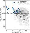 |
Fig. 1. sSFR as a function of the stellar mass of galaxies from the CIELO project (squares) and the MaNGA survey (gray dots). Blue squares indicate the selected sample, which includes CIELO galaxies with log(M⋆/M⊙)≥9 and log(sSFR)>−11 at z = 0. The unfilled black squares represent CIELO galaxies that were not included in the sample. The black dashed line marks the log(sSFR) = −11. |
This threshold allows us to select star-forming (SF) galaxies whose resolved scaling relations have been widely studied via observations and simulations (e.g., Sánchez et al. 2017; Trayford & Schaye 2019). This selection resulted in a sample of 21 SF galaxies (blue filled squares in Fig. 1). For this level of star formation activity, the Hα emission exceeds the minimum threshold established by Zhang et al. (2017) for minimizing contamination from diffuse ionized gas (DIG). Specifically, they found that MaNGA spaxels with Hα emission line surface density (ΣHα=Hα/Aspaxel, where Aspaxel is the spaxel area) above 1039 erg s−1 kpc−2 show reduced DIG contamination in their spectra. Therefore, we expected a minimal DIG impact on our sample.
For comparison, galaxies from the MaNGA survey, with log(M⋆/M⊙)≳9 (e.g., Ilbert et al. 2015; Spindler et al. 2018; Belfiore et al. 2018), have also been included (gray dots). As can be seen, this sample of CIELO galaxies is within the observational range although they tend to show a lower sSFR than the median at a given stellar mass. We refer to Tissera et al. (2025) for more details on the CIELO galaxies.
3. PRISMA pipeline
The numerical tool PRISMA allows us to generate synthetic spectra of simulated galaxies, facilitating the determination of their physical properties from an observational perspective. The following sections provide details of the design of PRISMA, as well as a description of the assumptions made for its construction.
3.1. Simulated data cubes
For the purpose stated above, we required resolved data cubes of the CIELO galaxies. We constructed grids that divide the projected mass distribution of each galaxy into hexagonal cells (hereafter, spaxels) with an area s. This scale is a free parameter within PRISMA and is, therefore, user-defined. For this work, we adopt s∼1 kpc2. The selection of this spaxel scale is motivated by the fact that we will confront the predicted rMZR with MaNGA results in the last section (Barrera-Ballesteros et al. 2016). However, the user can choose a different spaxel scale, as needed.
Furthermore, PRISMA enables the 3D rotation of galaxies using a user-defined angle. This feature allows for inclination corrections, providing a valuable opportunity to explore both local and global properties of galaxies with different inclinations. For simplicity, here we only analyzed face-on projections of the CIELO galaxies.
Figure 2 illustrates the two-dimensional properties of the gas distribution in a galaxy from the CIELO sample, considering its intrinsic information. The top row presents maps of the galaxy in a face-on orientation, while the bottom row displays maps in an edge-on orientation. The first column shows the spatial mass distribution of the gas component in the galaxy, while the second and third columns depict the line-of-sight (LoS) velocity and the velocity dispersion of the gas component, respectively (in km/s). The latter is calculated as the spread of the intrinsic velocities of the gas particles along the LoS within each spaxel, representing the deviation of the velocities from the mean velocity in that region. This figure reveals the morphology of the galaxy with a disk-like structure and discernible spiral arms, as can be seen in the upper panel of the first column. These features are consistent with the rotational patterns observed in the edge-on arrangement in the central column. Here, the expected red-shifted and blue-shifted velocity patterns of galaxies dominated by rotation are clearly detected.
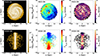 |
Fig. 2. Face-on (top row) and edge-on (bottom row) projected properties of the gas component in a CIELO galaxy, as an example. All properties are estimated using the intrinsic properties from the CIELO database and adopting an spaxel scale of s∼1 kpc2. The first column shows the gas-mass weighted distribution. The second column displays the velocity along the LoS for the gas component, whereas the third column illustrates the dispersion of this velocity. The FoV is adjusted to 60×60 kpc2 to encompass the entire galaxy. |
3.2. Synthetic spectra generation
After generating the simulated data cubes, the next step is to compute the spectra emitted by the stellar populations and SF regions contained in each spaxel. For this purpose, we employed the Python software Code Investigating GALaxy Emission (CIGALE, Burgarella et al. 2005; Noll et al. 2009; Boquien et al. 2019). This software facilitates spectrum generation and fitting by incorporating flexible models accounting for star formation history, stellar population emission, nebular emission, dust attenuation, and other properties.
We utilized CIGALE to generate synthetic spectra emitted from individual spaxels. Within each spaxel, these spectra are computed by considering the contributions of the stellar populations according to their ages and metallicities as well as nebular emission, arising from the gas surrounding the SF regions. The subsequent sections describe the methodology used to calculate these spectra by integrating CIGALE with the information provided by the simulations.
3.2.1. Star formation history
To generate the spectrum of each SSP, represented by a star particle, we assumed that its star formation history is quantified by the SFR, which is characterized by a single starburst event. The SFR is calculated based on the age provided by the simulation for each SSP. Then, to model the SFH of each SSP, we employed the sfhdelayed scheme, which incorporates the expression SFR =  , where t represents the age of the stellar population and τ denotes the e-folding time. The e-folding time indicates the rate at which the SFR decays. In other words, a larger τ implies a more prolonged period of star formation, while a smaller τ indicates a rapid decline in star formation following the initial burst. In this work, we chose a small τ = 0.1 Myr to represent a quasi-instantaneous birth of the entire stellar population.
3.2.2. Stellar population emission
Having established the SFH model for each SSP, the next step is to compute their spectra. For this purpose, we adopted the version of the Bruzual & Charlot (2003) stellar population synthesis models presented in Plat et al. (2019, CB19 models hereafter). The stellar ingredients used in the CB19 models (referred to as C&B models in some papers) are described in detail in Sánchez et al. (2022, see their Appendix A). With PRISMA we can adopt a Salpeter or a Chabrier IMF. In alignment with the CIELO specifications, we adopted the Chabrier IMF, while Z and the age of each SSP were directly extracted from the simulated data.
3.2.3. Nebular emission
When very massive stars form, they emit high-energy photons that ionize the surrounding gas. The ionized gas re-emits this energy in the form of emission lines and continuum, constituting what is known as nebular emission. This phenomenon depends on the chemical content and physical properties (electron density and temperature) of the interstellar medium and the ionization state of the gas.
To account for the contribution of nebular emission to the stellar spectra, we followed a similar approach implemented in Nanni et al. (2022), where distinct procedures are employed based on the age of each SSP. On one hand, we designated SSPs younger than 10 Myr as the young population, and the Z and t are taken directly from the simulations as mentioned above. The age threshold used in this study to separate between young and old SSPs is a user-defined parameter within our numerical tool. SSPs younger than this threshold are classified as the young population, and nebular emission is added to their spectra. SSPs older than this threshold are classified as the old population and do not include nebular emission in their spectra.
Additionally, we considered the SF gas as tracers of the regions of active star formation. SF gas particles are those that meet the conditions necessary for star formation (i.e., a temperature below 15 000 K and a density exceeding ρc = 7×10⁻²⁵ g cm−3, with ρc as the critical density), but because of the stochastic nature of star formation algorithm used, they have not been converted into star yet. In this case, we define fiducial young populations with fixed age of 105 yr. Properties such as mass, chemical abundances, density, position, and velocities are inherited by the fiducial SSP from the progenitor SF-gas particle. We assumed that both types of particles represent the SF regions and serve as the primary contributors to generating nebular emission. However, the user can chose whether to include them.
To model the nebular emission, we follow different steps depending on whether the young population is represented by an individual stellar particle or an SF-gas particle. In the first case, the closest gas particle to each individual stellar particle is assumed to represent its surrounding ionized gas. We defined the radius of the ionized gas cloud using the largest value between the smoothing length of the gas particle in question and the physical distance between it and the young SSP particle. This ensures that the population is contained within the gas clouds. In the second case, we assumed that SF-gas particles represent their own gas clouds. In other words, we modeled these gas clouds using the properties of each SF-gas particle, including its smoothing length as the radius of the SF region, as well as its metallicity and density. Considering these two cases, when the young population is represented either by an individual stellar particle or by a SF-gas particle, we find that the median ionized gas cloud size in our sample with intermediate (high) numerical resolution is 530 (363) pc, with the 25th and 25th percentiles at 490 (353) pc and 560 (373) pc, respectively. These values are consistent with the range of giant SF region sizes observed in the literature, which typically span from 100 pc to several hundred parsecs, depending on the galaxy type and environmental conditions (e.g., Hunt & Hirashita 2009; Kennicutt & Evans 2012; Grasha et al. 2022).
This assumption differentiates PRISMA from other tools generated in previous works (e.g., Trayford et al. 2017; Rodriguez-Gomez et al. 2018; Schulz et al. 2020; Nanni et al. 2022). In these studies, the modeling of nebular emission considers direct properties of stellar populations (e.g., their metallicity) rather than the gas properties. Additionally, these works assumed fixed parameters of the ISM, such as its pressure and compactness3, which are intricately linked to the ionized state of the ISM. The hypothesis we adopt in our work allows us to model the nebular emission based on the current ionization state and the direct properties of the gas surrounding each simulated SSP. Figure 3 illustrates our model, presenting the spectrum generated by old SSPs (upper inset panel) and the spectrum generated when nebular emissions from young SSPs are considered (lower inset panel).
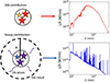 |
Fig. 3. Diagram of the model we adopted to add the emission lines to the spectra in PRISMA. The inset top panel shows the spectrum produced by stellar populations older than 10 Myr, which only depends on the CB19 stellar population synthesis models. The inset bottom panel displays the spectrum produced by stellar populations, which includes the CB19 SED models, and incorporates the nebular emission that is produced by the ionized gas cloud, which is represented by a sphere of radius R. |
CIGALE follows several steps to characterize nebular emission. Initially, leveraging the nebular templates proposed by Inoue (2011), it calculates the spectra of 124 emission lines as a function of U, the gas metallicity (Zgas) and the electron number density (ne). Each emission line within each spectrum is shaped with a Gaussian profile, utilizing a user-defined line width. Additionally, because there is a possibility that the rate of ionizing photons is reduced due to photon escape from the medium or photon absorption by dust located between the emitting star and the surrounding gas, CIGALE provides the capability to reduce the intensity of nebular emission lines by considering both the escape factor (fesc) and the dust factor (fdust).
Hence, the free parameters employed by CIGALE to describe the nebular emission are U, Zgas, ne, the line width, fesc, and fdust. In this context, we determined each of these parameters individually for each young SSP. We elaborate on how each parameter is defined based on the characteristics of the stellar populations and the surrounding gas below.
Ionization parameter: We computed the ionization parameter U following Equation (1), where R denotes the radius of the ionized gas cloud, fesc represents the escape fraction of photons that do not contribute to the ionization of the gas cloud, fdust corresponds to the fraction of photons that are absorbed by dust within the SF region, nHI is the numerical density of neutral hydrogen, c stands for the speed of light, and Qion represents the rate of photons ionizing the gas cloud.
 (1)
(1)
To calculate Qion, we must consider both the rate of ionizing photons emitted by each stellar population (Q*) and the maximum rate of ionizing photons that can be captured by the surrounding gas to become completely ionized (Qgas). On the one hand, Q* is calculated from the SSP models of CB19 that depends on the age, mass and metallicity of the stellar populations. On the other hand, Qgas is calculated by considering a simplified model where the gas cloud is composed only by hydrogen atoms, with a recombination rate αH∼2×10⁻¹³ cm3 s−1 (Ferland 1980) and an electron number density of ne. With that, the maximum ionizing photon rate that can be received by each gas particle is  .
.
Therefore, if Q*>Qgas, the gas cloud is considered to be completely ionized by the radiation emitted by the stellar population, and hence we have adopted, Qion=Qgas. Conversely, if Q*<Qgas, then the gas cloud is considered to be partially ionized, with Qion=Q*. In our sample, for all stellar populations we find that Q*>Qgas, so all SF regions in the sample are fully ionized.
Gas metallicity: We considered the metallicity of the gas cloud, which is directly provided by the simulation.
Electron number density: The simulation directly provides the initial electron number density (ne) of the gas particles surrounding each SSP. However, this initial ne does not account for the ionization impact of young stars.
When the gas cloud undergoes ionization, its electron density will vary in response to the incoming ionizing photons. As we specified earlier, when Q*>Qgas, the gas cloud is assumed to be completely ionized. In this case, considering that nHI is the initial neutral hydrogen density directly provided by the simulation, the resulting electron number density is given by  . In contrast, when Q*<Qgas,
  is determined based on the hydrogen atoms that have been ionized, considering the rate of ionizing photons emitted by the stellar population. Because Q*>Qgas for all stellar populations in our sample, we adopt
  , where both ne and nHI are quantities directly provided by the simulation.
To use CIGALE, ne is required to be binned between [10,100,1000] cm−3. Consequently, we assigned the simulated  values to the closest value specified by CIGALE. We investigate the impact of using ne=[10,100,1000] cm−3 on our calculations. Our findings revealed that these variations do not significantly alter the computed values of SFR and chemical abundances. In particular, we estimated a variation of 0.002 dex in the median SFR and a maximum variation of 0.06 dex in the median of the chemical abundances when using ne=[100] and ne=[1000] with respect to ne=[10], respectively. This latter estimation was obtained considering the five abundance indicators used in this paper (see Sect. 4.2).
Line width: The line width in the spectra reflects the kinematics of the gas within each region. The higher the velocity dispersion along the LoS, the broader the linewidth in the spectrum. To define these widths, we considered the standard deviation of the velocities along the LoS of all the gas particles that are located within each spaxel (see third column of Fig. 2).
fesc and fdust: Both parameters describe the fraction of photons that do not contribute to the nebular emission because they either escape (fesc) or are absorbed by dust within the SF region (fdust). We set the fesc = 0.10, which implies that 10% of the photons escape and do not ionize the gas cloud. This assumption is supported by observations at low redshift indicating that the escape fraction of Lyman-continuum photons does not exceed 10% (e.g., Bergvall et al. 2006; Plat et al. 2019), and references therein). To calculate fdust, we consider this factor as a free parameter, adjusting it to the value that produced spectra whose predicted SFR best reproduced the intrinsic SFR from the simulation. This approach enables the optimal recovery of the intrinsic SFR, which then allows us to incorporate a simple model to take into account the effect of dust inside the SF region. This dust is assumed to form a cocoon which absorbs a fraction of UV photons emitted by the young stellar population.
3.2.4. Dust attenuation
Dust within the ISM can modify galaxy spectra through processes such as absorption, scattering, and re-emission of photons, along the LoS. Dust absorbs UV to near-infrared photons and subsequently re-emits them in the mid- and far-infrared wavelengths. This principle of energy balance lies at the core of CIGALE, which allows the convolution of the spectra with the Calzetti attenuation law (Calzetti et al. 2000).
We investigated the effects of dust attenuation to assess how they could affect our calculations in Sect. 4.1.2. For this purpose, we created two datasets of spectra from the same sample of spaxels, considering different scenarios of dust absorption. The first dataset consists of spectra that are not attenuated by dust along the LoS. Therefore, they are only affected by dust within the H II regions, which absorbs the most energetic photons (regulated by the fdust parameter). The second dataset comprises spectra that are attenuated by both the dust within the H II regions and the dust in the ISM along the LoS. To model the impact of the latter, we used the Calzetti attenuation law by adopting E(B−V) = 0.3 mag. This approach provides a simplified representation compared to full radiative transfer treatments (e.g., Barrientos Acevedo et al. 2023). However, the analysis by Nanni et al. (2022) suggest that the effects of employing the Calzetti law are comparable to those obtained by using the Monte Carlo radiative transfer code SKIRT (Baes et al. 2011; Baes & Camps 2015).
4. Results and discussion
In this section, we explain how we applied PRISMA to the CIELO galaxies to compute the synthetic spectra with different dust recipes. We used five metallicity indicators to estimate the predicted abundances.
4.1. Fitting the free parameters of PRISMA
The first step is to choose the free parameters of PRISMA and to do so, we requested PRISMA to recover the intrinsic SFR from the Hα emission line flux.
4.1.1. Recovering the intrinsic SFR without dust attenuation
To calculate the intrinsic SFR per spaxel, we considered the total mass of the SSPs younger than t = 107 yr in a given spaxel, SFR=Myoung/t. Then, we determined the predicted SFR per spaxel by summing the synthetic Hα emission line flux generated by the SSPs within a given spaxel. Subsequently, we converted this Hα flux into the predicted SFR by using the calibration reported by Falcón-Barroso & Knapen (2013) as
 (2)
(2)
This equation is suitable for a Chabrier IMF (Kennicutt & Evans 2012). Therefore, it is well-aligned with CIELO specifications. Moreover, a comparable version of this relation was employed by Baker et al. (2023) to estimate the SFR in spatially resolved regions of MaNGA galaxies.
As previously mentioned, CIGALE utilizes various free parameters for characterizing nebular emission. Most of these parameters are derived from the intrinsic data of the simulation (e.g., log(U), Zgas, ne, and the line width), as described in previous sections. However, the fesc and fdust need to be determined. Since we are working with galaxies at z = 0, as we mentioned above, we assume fesc = 0.1. For the fdust, we take three different values: fdust = 0.4,0.5, and 0.6 to select the one that best traces the intrinsic SFR of the simulated sample. For all these three cases, we consider no attenuation by dust along the LoS.
Hence, we applied PRISMA with different fdust and estimated the predicted SFR and the SFR surface densities in each case, defined as ΣSFR=SFR/Aspaxel, where Aspaxel is the area of the spaxel. Then, we built histograms of ΣSFR and fit them by Gaussian distributions to better compared the results obtained from different fdust. Figure 4 shows the comparison of the Gaussian fittings to the intrinsic (black, solid line) and the predicted (dashed lines) ΣSFR for runs with fdust = 0.4,0.5,0.6 (green, red and blue, respectively). From this panel, we can see that the predicted distribution obtained with fdust = 0.5 is the one that best recovers the intrinsic SFR distribution.
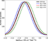 |
Fig. 4. Gaussian distributions fitted to the intrinsic SFR surface densities calculated by spaxel (black, solid lines) and to the corresponding predicted distributions obtained by applying PRISMA with fdust = 0.4, 0.5, and 0.6 (green, red and blue, dashed lines, respectively. |
Additionally, to achieve a better quantification, we calculated the relative difference between the intrinsic and predicted SFR. We define it as Δ(SFR) = (SFRpredicted−SFRintrinsic)/SFRintrinsic. For fdust = 0.5, which is the parameter that better reproduces the intrinsic values, we obtain a median Δ(SFR) = 0.06, with the 25th and 75th percentiles at 0.04 and 0.07, respectively. This indicates that PRISMA slightly overestimates the predicted SFR values with a relative error of 6%. Therefore, hereafter, we use fdust = 0.5 to generate the synthetic spectra of the CIELO sample, from which their resolved gas-phase metallicities will be derived for comparison with MaNGA observations.
Figure 5 illustrates examples of spectra computed by PRISMA (excluding dust attenuation along the LoS) for a face-on galaxy from the CIELO sample (which is different from the galaxy shown in Fig. 2). The left map displays the stellar mass distribution of the galaxy, with two highlighted spaxels, representing different regions. The red spaxel is located in an outer region of the disk, exclusively containing stellar populations older than 107 yr. Therefore, its composite spectrum has no emission lines (red spectrum). The blue spaxel is situated in one of the galaxy's spiral arms, containing both young and old stellar populations. The spectra produced by each of these populations are shown in the inset of the lower right panel of Fig. 5 in cyan and orange, respectively. Additionally, the contribution of the nebular emissions from the SF zones that enclose the young stars is displayed separately (violet spectrum). By accumulating all these contributions, we obtained the total spectrum emitted in this region as shown by the blue spectrum.
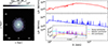 |
Fig. 5. Example of the composite spectra generated with PRISMA for two spaxels in a face-on galaxy of our CIELO sample. Left panel: Stellar mass-weighted distribution of a given galaxy, where two spaxels are highlighted in red and blue. The red spaxel contains only stellar populations older than 10 Myr, whereas the blue spaxel contains both old and younger stellar populations. Right panels: Corresponding spectra obtained with PRISMA from each of these spaxels (red and blue spectra, respectively). Additionally, the inset plot shows the old, young and nebular contributions (orange, cyan, and violet, respectively) that compose the total spectrum of the blue spaxel. These spectra were not attenuated by ISM dust along the LoS. |
4.1.2. Recovering the intrinsic SFR with dust attenuation
Until now, our discussion has not considered the absorption and re-emission effects of the computed spectra by dust that could be present in the ISM along the LoS. However, as discussed in Sect. 3.2.3, we have included a simple model for dust absorption within SF regions adopting the parameter fdust of CIGALE. In order to assess the impact of the ISM dust on our estimations, we have additionally produced spectra attenuated by the Calzetti law, following the procedure explained in Sect. 3.2.
To generate these attenuated spectra, the fdust value in PRISMA was taken as a free parameter in order to recover the intrinsic SFR from the attenuated spectra, similarly to was explained in the previous section. By reducing fdust from 0.5 to 0.1, we succeeded in recovering the intrinsic SFR of the sample, where we registered a change of  . With this value of fdust, only 10% of the photons are now absorbed by the dust within the SF regions while the rest of the attenuation effects are associated with the impact of dust along the LoS.
4.2. Estimating the gas-phase metallicity
Considering fesc = 0.1, fdust = 0.5 for the non-attenuated case and fesc = 0.1, fdust = 0.1 for the case run with the Calzetti law, we generated synthetic spectra with emission lines from the simulated sample. To estimate the intrinsic gas-phase metallicity for each spaxel, we used the intrinsic oxygen and hydrogen abundances provided directly by the simulation. Specifically, for each spaxel, we summed the total oxygen and hydrogen contributions from the gas particles assumed to represent SF regions. This total was then expressed in units of 12 + log(O/H). We focus exclusively on these regions because we later compare these intrinsic values with the estimates derived from their emission.
Furthermore, we derived the predicted gas-phase metallicity by employing emission line diagnostics that establish a connection between metallicity and emission line ratios originating from different chemical elements. Specifically, we utilized the N2, R23,  , O3N2 and N2O2 indicators, which are defined in Table 1. These indicators and their calibrations were chosen because they have been widely applied in observational studies (e.g., Pettini & Pagel 2004; Maiolino et al. 2008; Pérez-Montero & Contini 2009; Marino et al. 2013; Zhang et al. 2017; Curti et al. 2017, 2020; Laseter et al. 2024, among others). Additionally, they have been previously employed in simulation-based studies that generate synthetic spectra with emission lines, such as Garg et al. (2024) for SIMBA and Hirschmann et al. (2023) for IllustrisTNG simulations. A detailed discussion on them can be found in Kewley & Ellison (2008) and Conroy (2013), for example. We stress the fact that three different estimations for the SFR and the metallicity indicators will be considered: the intrinsic values, which are directly estimated from the simulations, the predicted values, given by PRISMA and, the observed values, calculated by using empirical and theoretical calibrations.
Line ratio definitions.
We first analyzed the non-attenuated case. Figure 6 shows the predicted N2, R23,  , O3N2 and O2N2 ratios derived from synthetic CIELO spectra as function of intrinsic 12+log(O/H) (black filled circles). We fit these data using a polynomial function of the form y=c0+c1x+c2x2, where x = 12 + log(O/H) and y is the respective line ratio. The fit to data lacking dust attenuation along the LoS is represented by the blue dashed lines, while the pink dashed curves show the fit to the data that were influenced by dust along the LoS. The shaded regions correspond to the 95% prediction intervals, which account for the expected dispersion of individual data points around the fitted polynomial. Table 2 displays the coefficients of the polynomial fits for all the metallicity indicators discussed above, for the spectra lacking dust attenuation along the LoS. This table also includes the lower and upper limits of the 95% prediction interval. Similar fits were performed for the attenuated case (see Table 3 for more details). Additionally, for better comparison, the red dots in the last panel of the figure show the distribution of the data attenuated using the Calzetti law.
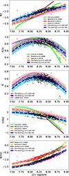 |
Fig. 6. Emission line ratios as a function of the intrinsic oxygen abundance for the sample data (black dots). The blue and pink dashed lines represent the best fits to the simulated data, considering synthetic spectra non-attenuated and attenuated by the Calzetti law, respectively. The shaded regions shows the 95% prediction intervals. The red dots in the last panel represent the attenuated data by the Calzetti law. The metallicity range of applicability of each literature calibration is reflected in the length of each relation. |
Predicted metallicity calibrations.
Predicted metallicity calibrations.
Figure 6 also includes the empirical calibrations derived by Marino et al. (2013), Curti et al. (2020), Sanders et al. (2017), Laseter et al. (2024), shown by the brown, light green, dark green, and purple solid lines, respectively. For comparison, the calibration reported by Garg et al. (2024, yellow, dashed line) is also shown, which was obtained using their own mocked emission method applied to the cosmological simulation SIMBA at z = 0 (Davé et al. 2019). Their predicted values were derived with the photoionization code Cloudy (Ferland et al. 2017) and considering the contributions from H II regions, post-AGB stars and DIGs. The relations provided by Maiolino et al. (2008) and Nagao et al. (2006) are semi-empirical calibrations (magenta and red lines, respectively). They used photoionization models to extend their empirical calibrations in the regime where there is no observational data available.
As indicated, the N2 and N2O2 curves, which directly depend on [N II]λ6584, show a significant increase with increasing oxygen abundance, which is mainly a consequence of secondary nitrogen4 production towards higher metallicities. The R23 and  ratios exhibit a more complex dependence on oxygen abundance because they show double-valued functions of metallicity. For metallicities below 12 + log(O/H) ∼ 8.2, these ratios increase for increasing O/H due to growing oxygen abundance. However, for higher metallicities, these ratios decrease as oxygen abundance rises. This is a result of efficient cooling of gas by heavy elements through metal lines, leading to fewer collisional excitations of optical transitions. Finally, the O3N2 ratio demonstrates a decreasing trend, aligning with the aforementioned arguments. As 12 + log(O/H) becomes higher, both the increase in [N II]λ6584 and the cooling of the gas cause the line ratio [O III]λ5007/[N II]λ6584 (i.e., O3N2) to decrease.
Overall, there is agreement between published calibrations and those predicted by our model for CIELO galaxies. However, the level of agreement varies depending on the calibrator used. Some differences exist for the O3N2 calibrations at 12+log(O/H)>8.5, where the simulated ratios are higher than expected from the empirical relations of Marino et al. (2013) and Curti et al. (2020), but agree better with the numerical predictions of Garg et al. (2024). A similar trend is observed for the R23 indicator at 12 + log(O/H) > 8.5, where our fit is in good agreement with the numerical predictions of Garg et al. (2024) and the semi-empirical calibration of Maiolino et al. (2008), but our slope differs from the calibration of Curti et al. (2020).
The differences between calibrations based on electron temperature (e.g., Curti et al. 2020) and those derived from photoionization models (e.g., Garg et al. 2024 and Maiolino et al. 2008 in the high metallicity regime) are well-documented in the literature (e.g., Stasińska 2005; Kewley & Ellison 2008; Cameron et al. 2023). At high metallicities, the Te method tends to saturate and significantly underestimate the true metallicity. This difference arises from temperature fluctuations and gradients, both within individual H II regions and across the entire galaxy (Stasińska 2005; Cameron et al. 2023).
Regarding our differences with Garg et al. (2024), we note that they did not consider active galactic nucleus (AGN) emission in their analysis, which makes it unlikely that AGNs contribute to the observed discrepancies, since our simulations neither include this process. However, their study does include the contribution from DIG, post-AGB stars, and incorporates dust in their simulations. DIG contamination alone may not fully account for the discrepancy as we only considered spaxels with ΣHα>1039 erg s−1 kpc−2, which are less affected according to Zhang et al. (2017). Additionally, for the N2O2 index as an example, our predictions closely match the line ratios presented in Nagao et al. (2006), but deviate from the calibrations of Sanders et al. (2018) and Garg et al. (2024) for 12+log(O/H)>8.15, where these calibrations have a steeper slope. The difference between the two observational calibrations can be explained by the fact that Sanders et al. (2018) applied a correction for DIG contamination whereas Nagao et al. (2006) did not. However, Garg et al. (2024) still obtained a slope similar to that of Sanders et al. (2018). This reinforces the idea that DIG contamination may not necessarily be the factor causing the difference between these line ratio predictions. Instead, as pointed out by Zhang et al. (2017), the N2O2 indicator is sensitive to the N/O ratio and temperature variations, which could explain the differences observed between the models. Also, the discrepancies with our models could arise because we are not considering the impact of post-AGB stars and our dust model is based on the Calzetti law. Moreover, it is important to bear in mind that oxygen abundance indicators involving nitrogen lines may also depend on the N/O ratio evolution in galaxies. In a future development, we plan to include a metal-dependent dust model.
The  indicator is a linear combination of R2 and R3 proposed by Laseter et al. (2024), representing a projection of both indicators to achieve a better fit for low metallicities. As shown in Fig. 6, for lower metallicities, our model aligns with the relation presented by Laseter et al. (2024). However, for the model without dust (blue segmented line), our estimates are shifted downward by approximately 0.08 dex. This could imply an overestimation of metallicities predicted by our
  calibration in comparison to those found by Laseter et al. (2024).
The lower panel of Fig. 7 shows the dependence of O3N2, R23,  , N2 and N2O2 on log(U) (bottom panel), considering the non-attenuated spectra by dust along LoS. The tracks represent the median values of the corresponding metallicity indicators per bin of log(U) (each bin contains at least 10 spaxels). The shaded regions represent the interquartile range of the line ratios in each ionization parameter bin, with the lower and upper limits corresponding to the 25th and 75th percentiles, respectively. The upper panel displays the distribution of the medians of the ionization parameters per spaxel in the simulated sample. Generally, the median simulated log(U) are in good agreement with spatially resolved data, as shown, for instance, by Mingozzi et al. (2020), Cameron et al. (2021) and Pérez-Montero et al. (2023) in the case of SF MaNGA galaxies.
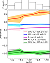 |
Fig. 7. Lower panel: Median predicted N2, R23, |

From Fig. 7, we can observe that the N2O2 index (green line) is only weakly sensitive to the ionization parameter. This relation yields a Spearman correlation coefficient of 0.05 (with p = 0.05). Many authors have reported that this indicator is not strongly dependent on the ionization parameter or variations in the shape of the ionizing spectrum (e.g., Dopita et al. 2000, 2013; Kewley & Dopita 2002; Zhang et al. 2017). This makes it a good metallicity indicator even in the presence of DIGs, as we mentioned previously. Additionally, this figure shows an increasing dependence of the O3N2 index on log(U), with a Spearman parameter of 0.26 (p<0.01). In the literature, it has been reported that this dependence on the ionization parameter may contribute to the scatter in the relationship between O3N2 with oxygen abundance displayed in Fig. 6 (e.g., Yin et al. 2007; Pérez-Montero & Contini 2009). This is because a decrease in ionization parameter leads to enhancement of [N II]/Hα and a decrease in [O III]/Hβ at the same time. This behavior should also imply the existence of an anti-correlation between N2 and log(U) (Pérez-Montero & Díaz 2005). In our sample we found a Spearman parameter of −0.17 (with p<0.01) between this indicator and log(U), which would confirm a weak anti-correlation between N2 and the ionization parameter. Finally, we found a positive dependence of R23 and  on ionization parameter, with Spearman parameters of 0.12 and 0.20, respectively (p<0.01). This indicates that the dependence of
  on the ionization parameter is stronger than that of R23.
Figure 8 depicts the predicted versus intrinsic metallicity values for the N2, R23,  , O3N2 and N2O2 indices, where the blue and pink contours represent the relations obtained by considering the non-attenuated and dust-attenuated spectra along the LoS, respectively. The contours give the density distribution of spaxels, where the inner, central and outer contours enclose 30, 50, and 90 per cent of the spaxels, respectively. For comparison the results obtained with empirical calibrations for N2 and O3N2 (Curti et al. 2020, cyan and red dots), R23 (Maiolino et al. 2008, yellow dots),
  (Laseter et al. 2024, magenta dots), and N2O2 (Nagao et al. 2006, green dots) are also included. To enhance the visualization, the relation y=x is overlaid (gray dashed line). The metallicity calculations were performed by using the applicability ranges of each literature calibration, as also shown in Fig. 6. Consequently, in the
  panel of Fig. 8, fewer metallicities are computed using the Laseter et al. (2024) calibration, as its applicability range is for 12+log(O/H)<8.4.
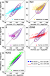 |
Fig. 8. Comparison between intrinsic gas-phase metallicities and values predicted from PRISMA spectra with fdust = 0.5 (blue contours) and with fdust = 0.1 and the Calzetti law (pink contours). The contours represent the density distributions of spaxels, where the inner, central and outer contours enclose the 30th, 50th, and 90th percentiles of the spaxels. The predicted abundances from the selected literature calibrations are also displayed (colored dots). The gray, dashed line depicts the 1:1 relation. |
From Fig. 8, we also note that the abundances derived using the semi-empirical N2O2 calibration of Nagao et al. (2006) (the lowest panel) are the ones that best align with those predicted by our model. In contrast, the metallicity estimates obtained with the other semi-empirical calibrations do not show the same level of agreement with our predictions. This could be related to the dependence of these indicators on log(U), as N2O2 exhibits a lower sensitivity to the ionization parameter, which may contribute to the closer agreement. This implies that, although PRISMA enables the estimation of log(U) using the intrinsic properties of the simulation, the current model should be considered with caution and is subject to improvements in future work. However, the observed performance confirms the robustness of the N2O2 index in the estimation of metallicities from synthetic spectra of simulations, particularly considering the complexity involved in determining the ionization state of the gas in the SF regions that contribute to such line ratios.
Finally, the use of our calibrations allowed us to estimate the predicted resolved scaling relation rMZR for our simulated sample. This can be seen in Fig. 9, where we display the intrinsic (black, solid lines) and the predicted (blue and pink dashed lines for non-attenuated and ISM dust-attenuated spectra, respectively) gas-phase abundances as a function of the surface stellar mass density (Σ*=M*/Aspaxel) per spaxel. To predict these values, we adopted our calibrations for N2, R23,  , N2O2, and O3N2. The shaded gray, blue and pink regions depict the respective 25th and 75th percentiles of the metallicities5 for the intrinsic and predicted estimations. We display the median relation reported by Barrera-Ballesteros et al. (2016, yellow, dashed line), which utilized disk galaxies from the MaNGA survey and employed the O3N2 index from Marino et al. (2013) to determine abundance estimations.
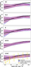 |
Fig. 9. Resolved mass-metallicity relation using intrinsic values from the CIELO simulations (black solid lines) and the calibrations of N2, R23, |

From Fig. 9, we can appreciate that PRISMA captures the intrinsic rMZR of CIELO for the five indicators studied in this paper overall. However, we note for O3N2,  , and R23 are the ones that depart the most from the intrinsic rMZR. Nevertheless, these differences are not larger of ∼0.15 dex. Hence, despite using a simple model to simulate H II regions and their nebular emission, PRISMA generates spectra that trace the intrinsic properties of the simulations.
Regarding the case with dust attenuation by using the Calzetti law, in Figs. 6, 8 and 9 we illustrate its impact on the generated spectra (pink curves and contours). From Fig. 6, we observe that the line ratios most influenced by considering dust effects along the LoS were the O3N2 and N2O2 indicators. However, based on the contours and the blue and pink lines in Figs. 8 and 9, the implementation of dust attenuation using the Calzetti law does not produce notable differences when predicting the metallicities of the simulated sample. In fact, the discrepancy between metallicities obtained from non-attenuated and ISM dust-attenuated spectra using the O3N2 indicator is less than ∼0.1 dex. Additionally, the metallicities predicted by the N2O2 indicator align with the intrinsic metallicities of the simulation, regardless of whether the spectra are non-attenuated or attenuated along the LoS.
However, caution should be exercised when estimating other galaxy properties, where the effects of dust attenuation and re-emission along the LoS may potentially be more significant.
5. Conclusions
We have developed a new numerical tool, PRISMA, which mocks IFU-like data cubes of simulated galaxies to estimate their physical properties through an observational approach. We used galaxies from the CIELO Project performed with intermediate and high resolution as test-beds. However, PRISMA can be applied to any type of simulations providing the expected parameters.
For each spaxel, we calculated the synthetic spectra considering the radiation emitted by the stellar populations and the nebular emission by the ionized gas near the youngest stellar populations. A fundamental aspect of PRISMA is that the nebular emission is calculated based on the properties of the gas surrounding the recently born stellar populations (see Nanni et al. 2022; Hirschmann et al. 2023; Garg et al. 2024, for alternative implementations). This allowed us to model log(U) by using the information on the gas component associated with the SF regions. Although this is a simplified scheme of a H II region, it yields a suitable representation of its properties.
Despite the fact that we have relied on simplified assumptions to model H II regions and their nebular emission, our scheme effectively produced spectra that closely recovered the intrinsic SFR and gas-phase metallicities of the galaxies within our sample. Specifically, we employed five metallicity indicators, N2, R23,  , O3N2, and N2O2, to derive the oxygen abundance, allowing us to compare the effectiveness of each indicator individually. We further analyzed the dependence of these line ratios on both metallicity and the ionization parameter.
We found that O3N2,  , and R23 show an increasing dependence on log(U), while N2 exhibits a decreasing trend. In contrast, N2O2 shows no significant correlation with log(U). Additionally, we developed new calibrations for these metallicity indices, which were then applied to derive the rMZR for our sample, yielding results consistent with the intrinsic rMZR.
In addition, we examined the impact of dust attenuation along the line of sight (LoS) on our results. For this, we adopted the Calzetti attenuation law (Calzetti et al. 2000) considering E(B−V) = 0.3 mag. From these spectra, we found that the O3N2 and N2O2 indicators are the most affected when applying the Calzetti law. However, when using these indicators to estimate the metallicities of the sample, there were no substantial discrepancies (<0.1 dex) compared to the estimates from spectra without ISM dust attenuation. In a future development, we expect to improve the dust modeling by including a more realistic representation.
These results confirm the robustness of PRISMA in retrieving the intrinsic properties of simulated galaxies, enabling a better comparison with observational data. In this way, this numerical tool can be used to test the impact of different observational issues, such as dust absorption, on generated spectra.
Data availability
The PRISMA code is publicly available at: https://github.com/AnellCornejoCardenas/PRISMA. In addition, example data for two galaxies are provided to illustrate the use of the code. The CIGALE software, can be downloaded and installed from https://cigale.lam.fr/.
Acknowledgments
We acknowledge the comments of the anonymous referee that contributed to improve this paper. We thanks Stephane Charlot for useful comments and discussion. AC thanks the Núcleo Milenio ERIS, Project N°NCN2021_017. ES acknowledges funding by Fondecyt-ANID Postdoctoral 2024 Project N°3240644 and thanks the Núcleo Milenio ERIS. PBT acknowledges partial funding by Fondecyt-ANID 1240465/2024, Núcleo Milenio ERIS, and ANID Basal Project FB210003. This project has received funding from the European Union Horizon 2020 Research and Innovation Programme under the Marie Sklodowska-Curie grant agreement No 734374-LACEGAL. MB gratefully acknowledges support from the ANID BASAL project FB210003 and from the FONDECYT regular grant 1211000. This work was supported by the French government through the France 2030 investment plan managed by the National Research Agency (ANR), as part of the Initiative of Excellence of Université Côte d’Azur under reference number ANR-15-IDEX-01. PJ acknowledges support form FONDECYT Regular 1231057 and Millennium Nucleus ERIS NCN2021_017. JV acknowledges financial support from the State Agency for Research of the Spanish MCIU through Center of Excellence Severo Ochoa award to the IAA CEX2021-001131-S funded by MCIN/AEI/10.13039/501100011033, and from grant PID2022-136598NB-C32 “Estallidos”. We acknowledge the use of the Ladgerda Cluster (Fondecyt 1200703/2020 hosted at the Institute for Astrophysics, Chile), the NLHPC (Centro de Modelamiento Matemático, Chile) and the Barcelona Supercomputer Center (Spain).
The metallicity (Z) is defined as the ratio between the mass of elements heavier than hydrogen and helium in a given baryonic component and its mass.
The optical radius is defined as the galactocentric radius that encloses ∼80 per cent of the stellar mass of a galaxy. This method allows for the estimation of the spatial extension of a simulated galaxy (Tissera et al. 2010) and adapts to the distributions of each galaxy. Hence, it is preferable over using a fixed aperture (Tissera et al. 2025).
The compactness is a measure of the density of an H II region, which depends on the star cluster mass and the ISM pressure.
Secondary nitrogen is produced from CNO elements present in stars, so that the nitrogen yield is metallicity-dependent (Clayton 1983).
The median rMZR are estimated in bins of Σ*, which contain at least 10 spaxels.
References
- Abdurroúf, Accetta, K., Aerts, C., et al. 2022, ApJS, 259, 35 [NASA ADS] [CrossRef] [Google Scholar]
- Baes, M., & Camps, P. 2015, Astron. Comput., 12, 33 [NASA ADS] [CrossRef] [Google Scholar]
- Baes, M., Verstappen, J., De Looze, I., et al. 2011, ApJS, 196, 22 [Google Scholar]
- Baker, W. M., Maiolino, R., Belfiore, F., et al. 2023, MNRAS, 519, 1149 [Google Scholar]
- Barrera-Ballesteros, J. K., Heckman, T. M., Zhu, G. B., et al. 2016, MNRAS, 463, 2513 [NASA ADS] [CrossRef] [Google Scholar]
- Barrientos Acevedo, D., van der Wel, A., Baes, M., et al. 2023, MNRAS, 524, 907 [NASA ADS] [CrossRef] [Google Scholar]
- Belfiore, F., Maiolino, R., Bundy, K., et al. 2018, MNRAS, 477, 3014 [Google Scholar]
- Bergvall, N., Zackrisson, E., Andersson, B. G., et al. 2006, A&A, 448, 513 [NASA ADS] [CrossRef] [EDP Sciences] [Google Scholar]
- Boardman, N., Zasowski, G., Newman, J. A., et al. 2022, MNRAS, 514, 2298 [NASA ADS] [CrossRef] [Google Scholar]
- Boquien, M., Burgarella, D., Roehlly, Y., et al. 2019, A&A, 622, A103 [NASA ADS] [CrossRef] [EDP Sciences] [Google Scholar]
- Bottrell, C., Torrey, P., Simard, L., & Ellison, S. L. 2017, MNRAS, 467, 2879 [NASA ADS] [CrossRef] [Google Scholar]
- Brinchmann, J., Charlot, S., White, S. D. M., et al. 2004, MNRAS, 351, 1151 [Google Scholar]
- Bruzual, G., & Charlot, S. 2003, MNRAS, 344, 1000 [NASA ADS] [CrossRef] [Google Scholar]
- Bundy, K., Bershady, M. A., Law, D. R., et al. 2015, ApJ, 798, 7 [Google Scholar]
- Burgarella, D., Buat, V., & Iglesias-Páramo, J. 2005, MNRAS, 360, 1413 [NASA ADS] [CrossRef] [Google Scholar]
- Calzetti, D., Armus, L., Bohlin, R. C., et al. 2000, ApJ, 533, 682 [NASA ADS] [CrossRef] [Google Scholar]
- Cameron, A. J., Fisher, D. B., McPherson, D., et al. 2021, ApJ, 918, L16 [NASA ADS] [CrossRef] [Google Scholar]
- Cameron, A. J., Katz, H., & Rey, M. P. 2023, MNRAS, 522, L89 [NASA ADS] [CrossRef] [Google Scholar]
- Casanueva-Villarreal, C., Tissera, P. B., Padilla, N., et al. 2024, A&A, 688, A183 [NASA ADS] [CrossRef] [EDP Sciences] [Google Scholar]
- Cataldi, P., Pedrosa, S. E., Tissera, P. B., et al. 2023, MNRAS, 523, 1919 [NASA ADS] [CrossRef] [Google Scholar]
- Chabrier, G. 2003, PASP, 115, 763 [Google Scholar]
- Clayton, D. D. 1983, Principles of stellar evolution and nucleosynthesis (Chicago: University of Chicago Press) [Google Scholar]
- Conroy, C. 2013, ARA&A, 51, 393 [NASA ADS] [CrossRef] [Google Scholar]
- Croom, S. M., Lawrence, J. S., Bland-Hawthorn, J., et al. 2012, MNRAS, 421, 872 [NASA ADS] [Google Scholar]
- Curti, M., Cresci, G., Mannucci, F., et al. 2017, MNRAS, 465, 1384 [Google Scholar]
- Curti, M., Mannucci, F., Cresci, G., & Maiolino, R. 2020, MNRAS, 491, 944 [Google Scholar]
- Daddi, E., Dickinson, M., Morrison, G., et al. 2007, ApJ, 670, 156 [NASA ADS] [CrossRef] [Google Scholar]
- Davé, R., Anglés-Alcázar, D., Narayanan, D., et al. 2019, MNRAS, 486, 2827 [Google Scholar]
- Davis, M., Efstathiou, G., Frenk, C. S., & White, S. D. M. 1985, ApJ, 292, 371 [Google Scholar]
- Dolag, K., Borgani, S., Murante, G., & Springel, V. 2009, MNRAS, 399, 497 [Google Scholar]
- Dopita, M. A., Kewley, L. J., Heisler, C. A., & Sutherland, R. S. 2000, ApJ, 542, 224 [NASA ADS] [CrossRef] [Google Scholar]
- Dopita, M. A., Sutherland, R. S., Nicholls, D. C., Kewley, L. J., & Vogt, F. P. A. 2013, ApJS, 208, 10 [NASA ADS] [CrossRef] [Google Scholar]
- Drory, N., Blanc, G. A., Kreckel, K., et al. 2024, AJ, 168, 198 [NASA ADS] [CrossRef] [Google Scholar]
- Emsellem, E., Schinnerer, E., Santoro, F., et al. 2022, A&A, 659, A191 [NASA ADS] [CrossRef] [EDP Sciences] [Google Scholar]
- Falcón-Barroso, J., & Knapen, J. H. 2013, Secular Evolution of Galaxies (Cambridge, UK: Cambridge University) [Google Scholar]
- Ferland, G. J. 1980, PASP, 92, 596 [CrossRef] [Google Scholar]
- Ferland, G. J., Chatzikos, M., Guzmán, F., et al. 2017, Rev. Mex. Astron. Astrofis., 53, 385 [NASA ADS] [Google Scholar]
- Furlong, M., Bower, R. G., Theuns, T., et al. 2015, MNRAS, 450, 4486 [Google Scholar]
- Garg, P., Narayanan, D., Sanders, R. L., et al. 2024, ApJ, 972, 113 [NASA ADS] [CrossRef] [Google Scholar]
- Gonzalez-Jara, J., Tissera, P. B., Monachesi, A., et al. 2025, A&A, 693, A282 [NASA ADS] [CrossRef] [EDP Sciences] [Google Scholar]
- Grasha, K., Chen, Q. H., Battisti, A. J., et al. 2022, ApJ, 929, 118 [NASA ADS] [CrossRef] [Google Scholar]
- Hirschmann, M., Charlot, S., & Somerville, R. S. 2023, MNRAS, 526, 3504 [NASA ADS] [CrossRef] [Google Scholar]
- Hunt, L. K., & Hirashita, H. 2009, A&A, 507, 1327 [NASA ADS] [CrossRef] [EDP Sciences] [Google Scholar]
- Ilbert, O., Arnouts, S., Le Floc’h, E., et al. 2015, A&A, 579, A2 [NASA ADS] [CrossRef] [EDP Sciences] [Google Scholar]
- Inoue, A. K. 2011, MNRAS, 415, 2920 [NASA ADS] [CrossRef] [Google Scholar]
- Iwamoto, K., Brachwitz, F., Nomoto, K., et al. 1999, ApJS, 125, 439 [NASA ADS] [CrossRef] [Google Scholar]
- Kennicutt, R. C. Jr. 1983, ApJ, 272, 54 [NASA ADS] [CrossRef] [Google Scholar]
- Kennicutt, R. C., & Evans, N. J. 2012, ARA&A, 50, 531 [NASA ADS] [CrossRef] [Google Scholar]
- Kewley, L. J., & Dopita, M. A. 2002, ApJS, 142, 35 [Google Scholar]
- Kewley, L. J., & Ellison, S. L. 2008, ApJ, 681, 1183 [Google Scholar]
- Laseter, I. H., Maseda, M. V., Curti, M., et al. 2024, A&A, 681, A70 [NASA ADS] [CrossRef] [EDP Sciences] [Google Scholar]
- Maier, C., Lilly, S. J., Ziegler, B. L., et al. 2014, ApJ, 792, 3 [NASA ADS] [CrossRef] [Google Scholar]
- Maiolino, R., Nagao, T., Grazian, A., et al. 2008, A&A, 488, 463 [NASA ADS] [CrossRef] [EDP Sciences] [Google Scholar]
- Maraston, C., Hill, L., Thomas, D., et al. 2020, MNRAS, 496, 2962 [Google Scholar]
- Marino, R. A., Rosales-Ortega, F. F., Sánchez, S. F., et al. 2013, A&A, 559, A114 [NASA ADS] [CrossRef] [EDP Sciences] [Google Scholar]
- Mingozzi, M., Belfiore, F., Cresci, G., et al. 2020, A&A, 636, A42 [NASA ADS] [CrossRef] [EDP Sciences] [Google Scholar]
- Mosconi, M. B., Tissera, P. B., Lambas, D. G., & Cora, S. A. 2001, MNRAS, 325, 34 [NASA ADS] [CrossRef] [Google Scholar]
- Nagao, T., Maiolino, R., & Marconi, A. 2006, A&A, 459, 85 [NASA ADS] [CrossRef] [EDP Sciences] [Google Scholar]
- Nanni, L., Thomas, D., Trayford, J., et al. 2022, MNRAS, 515, 320 [CrossRef] [Google Scholar]
- Nelson, D., Springel, V., Pillepich, A., et al. 2019, Comput. Astrophys. Cosmol., 6, 2 [Google Scholar]
- Noll, S., Burgarella, D., Giovannoli, E., et al. 2009, A&A, 507, 1793 [NASA ADS] [CrossRef] [EDP Sciences] [Google Scholar]
- Pedrosa, S. E., & Tissera, P. B. 2015, A&A, 584, A43 [NASA ADS] [CrossRef] [EDP Sciences] [Google Scholar]
- Peng, Y. -J., Lilly, S. J., Kovač, K., et al. 2010, ApJ, 721, 193 [NASA ADS] [CrossRef] [Google Scholar]
- Pérez-Montero, E., & Contini, T. 2009, MNRAS, 398, 949 [CrossRef] [Google Scholar]
- Pérez-Montero, E., & Díaz, A. I. 2005, MNRAS, 361, 1063 [CrossRef] [Google Scholar]
- Pérez-Montero, E., Zinchenko, I. A., Vílchez, J. M., et al. 2023, A&A, 669, A88 [NASA ADS] [CrossRef] [EDP Sciences] [Google Scholar]
- Pettini, M., & Pagel, B. E. J. 2004, MNRAS, 348, L59 [NASA ADS] [CrossRef] [Google Scholar]
- Planck Collaboration I. 2014, A&A, 571, A1 [NASA ADS] [CrossRef] [EDP Sciences] [Google Scholar]
- Plat, A., Charlot, S., Bruzual, G., et al. 2019, MNRAS, 490, 978 [Google Scholar]
- Renzini, A., & Peng, Y. -J. 2015, ApJ, 801, L29 [NASA ADS] [CrossRef] [Google Scholar]
- Rodríguez, S., Garcia Lambas, D., Padilla, N. D., et al. 2022, MNRAS, 514, 6157 [CrossRef] [Google Scholar]
- Rodriguez-Gomez, V., Snyder, G. F., Lotz, J. M., et al. 2018, MNRAS, 483, 4140 [Google Scholar]
- Sánchez, S. F., Kennicutt, R. C., Gil de Paz, A., et al. 2012, A&A, 538, A8 [Google Scholar]
- Sánchez, S. F., Barrera-Ballesteros, J. K., Sánchez-Menguiano, L., et al. 2017, MNRAS, 469, 2121 [CrossRef] [Google Scholar]
- Sánchez, S. F., Walcher, C. J., Lopez-Cobá, C., et al. 2021, Rev. Mex. Astron. Astrofis., 57, 3 [Google Scholar]
- Sánchez, S. F., Barrera-Ballesteros, J. K., Lacerda, E., et al. 2022, ApJS, 262, 36 [CrossRef] [Google Scholar]
- Sánchez-Menguiano, L., Sánchez, S. F., Pérez, I., et al. 2018, A&A, 609, A119 [NASA ADS] [CrossRef] [EDP Sciences] [Google Scholar]
- Sanders, R. L., Shapley, A. E., Zhang, K., & Yan, R. 2017, ApJ, 850, 136 [NASA ADS] [CrossRef] [Google Scholar]
- Sanders, R. L., Shapley, A. E., Kriek, M., et al. 2018, ApJ, 858, 99 [NASA ADS] [CrossRef] [Google Scholar]
- Scannapieco, C., Tissera, P. B., White, S. D. M., & Springel, V. 2005, MNRAS, 364, 552 [NASA ADS] [CrossRef] [Google Scholar]
- Scannapieco, C., Tissera, P. B., White, S. D. M., & Springel, V. 2006, MNRAS, 371, 1125 [NASA ADS] [CrossRef] [Google Scholar]
- Schaye, J., Crain, R. A., Bower, R. G., et al. 2015, MNRAS, 446, 521 [Google Scholar]
- Schulz, S., Popping, G., Pillepich, A., et al. 2020, MNRAS, 497, 4773 [NASA ADS] [CrossRef] [Google Scholar]
- Snyder, G. F., Torrey, P., Lotz, J. M., et al. 2015, MNRAS, 454, 1886 [NASA ADS] [CrossRef] [Google Scholar]
- Spindler, A., Wake, D., Belfiore, F., et al. 2018, MNRAS, 476, 580 [NASA ADS] [CrossRef] [Google Scholar]
- Springel, V., Yoshida, N., & White, S. D. M. 2001, New Astron., 6, 79 [Google Scholar]
- Stasińska, G. 2005, A&A, 434, 507 [NASA ADS] [CrossRef] [EDP Sciences] [Google Scholar]
- Tapia-Contreras, B., Tissera, P. B., Sillero, E., et al. 2025, A&A, in press, https://doi.org/10.1051/0004-6361/202554013 [Google Scholar]
- Tissera, P. B., Lambas, D. G., & Abadi, M. G. 1997, MNRAS, 286, 384 [NASA ADS] [Google Scholar]
- Tissera, P. B., White, S. D. M., Pedrosa, S., & Scannapieco, C. 2010, MNRAS, 406, 922 [NASA ADS] [Google Scholar]
- Tissera, P. B., Bignone, L., Gonzalez-Jara, J., et al. 2025, A&A, 697, A134 [NASA ADS] [CrossRef] [EDP Sciences] [Google Scholar]
- Torrey, P., Snyder, G. F., Vogelsberger, M., et al. 2015, MNRAS, 447, 2753 [NASA ADS] [CrossRef] [Google Scholar]
- Trayford, J. W., & Schaye, J. 2019, MNRAS, 485, 5715 [NASA ADS] [CrossRef] [Google Scholar]
- Trayford, J. W., Theuns, T., Bower, R. G., et al. 2015, MNRAS, 452, 2879 [NASA ADS] [CrossRef] [Google Scholar]
- Trayford, J. W., Camps, P., Theuns, T., et al. 2017, MNRAS, 470, 771 [NASA ADS] [CrossRef] [Google Scholar]
- Tremonti, C. A., Heckman, T. M., Kauffmann, G., et al. 2004, ApJ, 613, 898 [Google Scholar]
- van de Sande, J., Fraser-McKelvie, A., Fisher, D. B., et al. 2024, in Early Disk-Galaxy Formation from JWST to the Milky Way, eds. F. Tabatabaei, B. Barbuy, & Y. S. Ting, IAU Symposium, 377, 27 [Google Scholar]
- Woosley, S. E., & Weaver, T. A. 1995, ApJS, 101, 181 [Google Scholar]
- Yan, R., Chen, Y., Lazarz, D., et al. 2019, ApJ, 883, 175 [Google Scholar]
- Yao, Y., Chen, G., Liu, H., et al. 2022, A&A, 661, A112 [NASA ADS] [CrossRef] [EDP Sciences] [Google Scholar]
- Yin, S. Y., Liang, Y. C., Hammer, F., et al. 2007, A&A, 462, 535 [NASA ADS] [CrossRef] [EDP Sciences] [Google Scholar]
- Zahid, H. J., Dima, G. I., Kudritzki, R. -P., et al. 2014, ApJ, 791, 130 [NASA ADS] [CrossRef] [Google Scholar]
- Zhang, K., Yan, R., Bundy, K., et al. 2017, MNRAS, 466, 3217 [NASA ADS] [CrossRef] [Google Scholar]
All Tables
All Figures
|
Fig. 1. sSFR as a function of the stellar mass of galaxies from the CIELO project (squares) and the MaNGA survey (gray dots). Blue squares indicate the selected sample, which includes CIELO galaxies with log(M⋆/M⊙)≥9 and log(sSFR)>−11 at z = 0. The unfilled black squares represent CIELO galaxies that were not included in the sample. The black dashed line marks the log(sSFR) = −11. |
| In the text | |
|
Fig. 2. Face-on (top row) and edge-on (bottom row) projected properties of the gas component in a CIELO galaxy, as an example. All properties are estimated using the intrinsic properties from the CIELO database and adopting an spaxel scale of s∼1 kpc2. The first column shows the gas-mass weighted distribution. The second column displays the velocity along the LoS for the gas component, whereas the third column illustrates the dispersion of this velocity. The FoV is adjusted to 60×60 kpc2 to encompass the entire galaxy. |
| In the text | |
|
Fig. 3. Diagram of the model we adopted to add the emission lines to the spectra in PRISMA. The inset top panel shows the spectrum produced by stellar populations older than 10 Myr, which only depends on the CB19 stellar population synthesis models. The inset bottom panel displays the spectrum produced by stellar populations, which includes the CB19 SED models, and incorporates the nebular emission that is produced by the ionized gas cloud, which is represented by a sphere of radius R. |
| In the text | |
|
Fig. 4. Gaussian distributions fitted to the intrinsic SFR surface densities calculated by spaxel (black, solid lines) and to the corresponding predicted distributions obtained by applying PRISMA with fdust = 0.4, 0.5, and 0.6 (green, red and blue, dashed lines, respectively. |
| In the text | |
|
Fig. 5. Example of the composite spectra generated with PRISMA for two spaxels in a face-on galaxy of our CIELO sample. Left panel: Stellar mass-weighted distribution of a given galaxy, where two spaxels are highlighted in red and blue. The red spaxel contains only stellar populations older than 10 Myr, whereas the blue spaxel contains both old and younger stellar populations. Right panels: Corresponding spectra obtained with PRISMA from each of these spaxels (red and blue spectra, respectively). Additionally, the inset plot shows the old, young and nebular contributions (orange, cyan, and violet, respectively) that compose the total spectrum of the blue spaxel. These spectra were not attenuated by ISM dust along the LoS. |
| In the text | |
|
Fig. 6. Emission line ratios as a function of the intrinsic oxygen abundance for the sample data (black dots). The blue and pink dashed lines represent the best fits to the simulated data, considering synthetic spectra non-attenuated and attenuated by the Calzetti law, respectively. The shaded regions shows the 95% prediction intervals. The red dots in the last panel represent the attenuated data by the Calzetti law. The metallicity range of applicability of each literature calibration is reflected in the length of each relation. |
| In the text | |
|
Fig. 7. Lower panel: Median predicted N2, R23, |
| In the text | |
|
Fig. 8. Comparison between intrinsic gas-phase metallicities and values predicted from PRISMA spectra with fdust = 0.5 (blue contours) and with fdust = 0.1 and the Calzetti law (pink contours). The contours represent the density distributions of spaxels, where the inner, central and outer contours enclose the 30th, 50th, and 90th percentiles of the spaxels. The predicted abundances from the selected literature calibrations are also displayed (colored dots). The gray, dashed line depicts the 1:1 relation. |
| In the text | |
|
Fig. 9. Resolved mass-metallicity relation using intrinsic values from the CIELO simulations (black solid lines) and the calibrations of N2, R23, |
| In the text | |
Current usage metrics show cumulative count of Article Views (full-text article views including HTML views, PDF and ePub downloads, according to the available data) and Abstracts Views on Vision4Press platform.
Data correspond to usage on the plateform after 2015. The current usage metrics is available 48-96 hours after online publication and is updated daily on week days.
Initial download of the metrics may take a while.