| Issue |
A&A
Volume 692, December 2024
|
|
|---|---|---|
| Article Number | A105 | |
| Number of page(s) | 15 | |
| Section | Extragalactic astronomy | |
| DOI | https://doi.org/10.1051/0004-6361/202450916 | |
| Published online | 03 December 2024 | |
A multi-wavelength overview of the giant spiral UGC 2885
1
Department of Physics & Astronomy, University of Western Ontario, 1151 Richmond Street, London, Ontario, Canada
2
Institute for Earth & Space Exploration, University of Western Ontario, 1151 Richmond Street, London, Ontario, Canada
3
Center for Interdisciplinary Exploration and Research in Astrophysics (CIERA) and Department of Physics and Astronomy, Northwestern University, Evanston, IL 60208, USA
4
Department of Space, Earth and Environment, Chalmers University of Technology, Onsala Space Observatory, 439 92 Onsala, Sweden
5
Department of Physics & Astronomy, University of Louisville, Natural Science Building 102, Louisville, KY 40292, USA
6
Department of Astronomy, University of Massachusetts, Amherst, MA 01003, USA
7
The SETI Institute, Mountain View, California 94043, USA
⋆ Corresponding author; This email address is being protected from spambots. You need JavaScript enabled to view it.
Received:
29
May
2024
Accepted:
14
October
2024
Abstract
Context. UGC 2885 (z = 0.01935) is one of the largest and most massive galaxies in the local Universe, yet it has an undisturbed spiral structure, which is unexpected for such an object and is not predicted by cosmological simulations. Understanding the detailed properties of extreme systems such as UGC 2885 can provide insight into the limits of scaling relations and the physical processes driving galaxy evolution.
Aims. Our goal is to understand whether UGC 2885 has followed a similar evolutionary path as other high-mass galaxies by examining its place in the fundamental metallicity relation and on the star-forming main sequence.
Methods. We present new observations of UGC 2885 with the Canada-France-Hawaii Telescope and the Institut de radioastronomie millimétrique 30 m telescope. We used these novel data to calculate metallicity and molecular hydrogen mass values, respectively. We estimated the stellar mass (M⋆) and star formation rate (SFR) based on mid-infrared observations with the Wide-field Infrared Survey Explorer.
Results. We find global metallicities Z = 9.28, 9.08, and 8.74 at the 25 kpc ellipsoid from the N2O2, R23, and O3N2 indices, respectively. This puts UGC 2885 at the high end of the galaxy metallicity distribution. We find a molecular hydrogen mass of MH2 = 1.89 ± 0.24 × 10¹¹ M⊙, a SFR of 1.63 ± 0.72 M⊙ yr−1, and a stellar mass of 4.83 ± 1.52 × 10¹¹ M⊙, which gives a star formation efficiency (SFR/MH2) of 8.67 ± 4.20 × 10¹² yr−1. This indicates that UGC 2885 has an extremely high molecular gas content compared to known samples of star-forming galaxies (∼100 times more) and a relatively low SFR for its current gas content.
Conclusions. We conclude that UGC 2885 has gone through cycles of star formation periods, which increased its stellar mass and metallicity to its current state. The mechanisms that are fuelling the current molecular gas reservoir and keeping the galaxy from producing stars remain uncertain. We discuss the possibility that a molecular bar is quenching star-forming activity.
Key words: galaxies: evolution / galaxies: individual: UGC 2885 / galaxies: star formation
© The Authors 2024
 Open Access article, published by EDP Sciences, under the terms of the Creative Commons Attribution License (https://creativecommons.org/licenses/by/4.0), which permits unrestricted use, distribution, and reproduction in any medium, provided the original work is properly cited.
This article is published in open access under the Subscribe to Open model. This email address is being protected from spambots. You need JavaScript enabled to view it. to support open access publication.
1. Introduction
The galaxy UGC 2885, or Rubin’s Galaxy, is notable in the local Universe (z < 0.1) for being the largest and most massive spiral (Rubin et al. 1980; Romanishin 1983). UGC 2885 has four defined arms and traces of star formation activity along them (Hunter et al. 2013). With an estimated radius of 122 kpc and a total mass of  (Rubin et al. 1980), this object challenges our understanding of galactic formation and evolution: cosmological simulations (e.g. Vogelsberger et al. 2014; Snyder et al. 2015) do not predict the existence of such galaxies. The higher end of the mass distribution of galaxies is thought to have evolved via the accretion of gas due to mergers with companion or generally nearby systems (Lacey & Cole 1993; Kereš et al. 2005). This might not be the case for UGC 2885, as it is located in an isolated environment, is essentially bulge-free, and shows no sign of perturbed morphology.
Another consequence of galaxy growth via mergers is the presence of an active galactic nucleus (AGN) since mergers diminish angular momentum and contribute to black hole accretion (Dietrich et al. 2018; Gao et al. 2020). Holwerda et al. (2021) compared a UGC 2885 spectrum predicted by machine learning to spectra obtained from optical observations with VIRUS-P (Visible Integral-field Replicable Unit Spectrograph – Prototype; Hill et al. 2008) and MMT/Binospec. They find good qualitative agreement and conclude that both the predicted and observed line ratios (O III/Hβ versus N II/Hα and O III/Hβ versus S II/Hα) were consistent with AGN activity. The mid-infrared colour of UGC 2885’s central region was not sufficiently red to identify it as an AGN, and Holwerda et al. (2021) suggest that a mid-infrared AGN signal is likely diluted by the large point spread function.
Although massive, UGC 2885 does not meet the criteria to be considered a ‘super spiral’ (Ogle et al. 2016). Super-spiral galaxies are generally found in richer environments and have higher star formation rates (SFRs) than those reported for Rubin’s Galaxy: 5 − 70 M⊙ yr−1 for super spirals (Ogle et al. 2016) versus 2.47 M⊙ yr−1 for UGC 2885 (Hunter et al. 2013)1. Another analogue classification is the group of giant low-surface-brightness disc galaxies (gLSBs; Saburova et al. 2021). These objects are remarkably isolated, contain large reservoirs of gas, and have extremely low SFRs (a mean SFR of 0.88 M⊙ yr−1; Du et al. 2023). UGC 2885 has a higher SFR and brighter surface brightness than a typical gLSB (Holwerda et al. 2021).
Previous studies have acknowledged that UGC 2885 lies on the extreme ends of the mass and size distributions for local galaxies. 21 cm line observations using the Westerbork Synthesis Radio Telescope (WSRT) probed the rotation curve derived from UGC 2885’s neutral hydrogen (H I) emission, corroborating the exceptional baryonic mass and morphological symmetry (Lewis 1985; Roelfsema & Allen 1985). Canzian et al. (1993) obtained Hα imaging data of UGC 2885 using the Isaac Newton Telescope and found that underlying density waves, possibly driven by the galaxy’s enormous mass, may contribute to the stability of its disc. Expanding on the same optical line with the Kitt Peak National Observatory (KPNO), Hunter et al. (2013) identified ionised hydrogen (H II) regions across 5.6 disc scale lengths (∼70 kpc) as well as detached star-forming regions at the end of the galactic arms.
In this paper we aim to provide an overview of some of Rubin’s Galaxy’s properties using a range of observations. By representing a system at the upper bounds of mass and size in the nearby Universe, UGC 2885 could be an important tool for better understanding galaxy formation and how certain properties can evolve in an isolated environment. Although it has previously been studied in the radio and optical regimes, we extend the results by diving into specific lines within those bands. In the millimetre regime, we analysed CO(1−0) (rest frequency 115.27 GHz) line observations, a probe of molecular hydrogen (H2), and in the optical we studied the O IIλ3727, Hβλ4861, O III4959 + 5007, Hαλ6563, N II6548 + 6583, and S II6717 + 6731 emission lines, analysing their line ratios to provide insight into the metallicity and, although not the major focus of this work, the nuclear activity. We aim to answer the following questions: How does UGC 2885 compare to other massive spiral galaxies on the stellar mass-SFR plane? Does it seem to evolve the same way as normal-sized spirals? What are the possible evolution scenarios that made this galaxy grow to its great mass without its losing spiral structure and active star formation?
This paper is organised as follows: Section 2 discusses the archival and novel observations of UGC 2885, as well as how each specific dataset was processed and analysed. Sections 3–5 discuss the estimation of physical properties from the observational data. In Sect. 6 we explore the results of our analysis, focusing specifically on the new information found – molecular gas content and the stellar population – and its relation to the current understanding of this object’s formation and evolution. Section 7 summarises the findings and suggests future work.
2. Observations
Table 1 summarises some of UGC 2885’s properties. To place UGC 2885 in context, Fig. 1 compares the galaxy’s size and stellar mass to those of 5.3 × 10⁴ local (z < 0.05) star-forming galaxies in the combination of the GALEX-SDSS-WISE Legacy Catalog (Salim et al. 2016) and Siena Galaxy Atlas (Moustakas et al. 2023). It is one of the largest and most massive galaxies in the local Universe. For visual reference, Fig. 2 shows a colour composite of Hubble Space Telescope (HST) Wide Field Camera 3 (WFC3) images of UGC 2885 (proposal ID: 15107, PI: Holwerda), constructed with the REPROJECT and MAKE_LUPTON_RGB packages of the Astropy library. Detailed analysis of the HST images, including surface brightness profile fitting and star cluster population analysis will be presented elsewhere (Holwerda et al., in prep.; see also Sect. 6.9).
Basic properties of UGC 2885.
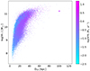 |
Fig. 1. Size–stellar mass relation for local star-forming galaxies in the GALEX-SDSS-WISE Legacy Catalog (Salim et al. 2016) and Siena Galaxy Atlas (Moustakas et al. 2023). The large star indicates the position of UGC 2885, with the stellar mass as reported by Di Teodoro et al. (2023), the SFR as reported by Hunter et al. (2013), D25 from the HyperLEDA database, and the distance given in Table 1. |
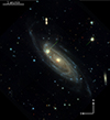 |
Fig. 2. Colour composite of HST/WFC3 images of UGC 2885 (F814W, F606W, and F475W in red, green, and blue, respectively). A bright foreground star (HD279085, V = 10.7) is inconveniently superimposed on the disc. |
Our data consist of a multi-wavelength collection of images and datacubes that spans from the optical to the radio domain, mixing both archival and novel observations summarised in Table 2. Luminosities and subsequent properties were calculated assuming a flat cosmology with H0 = 70 km s−1 Mpc−1, Ωm = 0.3 and ΩΛ = 0.7. At the distance of UGC 2885, 1′′ corresponds to a physical projected distance of 409 pc; UGC 2885’s half-light radius of 22 kpc subtends  .
.
Observational data.
2.1. Optical: SITELLE
We observed UGC 2885 with the Canada-France-Hawaii Telescope (CFHT) SITELLE (Spectromètre Imageur à Transformée de Fourier pour l’Etude en Long et en Large de raies d’Emission), an imaging Fourier transform spectrograph specifically designed to detect prominent emission lines in the visible spectrum (Drissen et al. 2019). SITELLE provides an 11′×11′ field of view (FOV) with a plate scale of  per pixel. This FOV allowed us to achieve a comprehensive single-field view of the galaxy and therefore datacubes covering three relatively narrow wavelength ranges. Observations were carried out under proposal IDs 19BC13 and 20BC05 with observations performed on 30 September 2019, 19 November 2020, and 11 December 2020. Seeing during the observation dates varied between approximately 1′′ and
  full width at half maximum (FWHM).
We used the CFHT-provided SITELLE data (Martin et al. 2012, processed with the ORBS (Outil de Réduction Binoculaire pour SITELLE) pipeline) and carried out further analysis with LUCI (Rhea et al. 2021a, 2021b). ORBS-processed deep white-light images were utilised to view details of the galaxy while LUCI was used to produce line flux maps for each strong emission line from the ORBS-processed datacubes. We followed the template Python notebooks provided in LUCI (BasicExample, SN1, and SN2), adopting the suggested parameters for the line shape fitting function of sinc convolved with Gaussian for SN1 and pure Gaussian for SN2 and SN3. The templates were changed to reflect the spectral resolution used in our observation (Table 2), the galaxy’s redshift, and our choice to use 2 × 2 pixel binning. Binning doubles the signal-to-noise ratio (S/N) and reduces processing time, at a cost of reducing the spatial resolution. The observations for each filter were taken on separate dates, so the datacubes did not have identical pointing. We adjusted the x and y pixel parameters in the LUCI fit_cube function, using bright stars as a guide, to ensure alignment between all three datacubes. The aligned line flux maps (and corresponding uncertainty maps) generated with LUCI were combined into line ratio maps to measure metallicity (see Sect. 3) and nuclear line ratios (Appendix A).
The ORBS-processed deep white light images (Fig. 3) reveal similar galaxy structure to the HST images (Fig. 2), although at about 10 times lower spatial resolution (about 400 pc for SITELLE and 40 pc for HST). The white light images are sufficient for use in defining three elliptical apertures with which to measure spatial variation in metallicity. The inner aperture focuses on the central bulge while the largest ellipse allows a determination of the global metallicity. We opted not to analyse the outer spiral arms due to their low surface brightness. As Fig. 3 shows, we also masked the bright foreground star that appears in the outer ellipse.
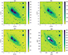 |
Fig. 3. ORBS-processed deep white light flux maps in SN1 (363–386 nm), SN2 (482–513 nm), and SN3 (647–685 nm) filters. Bottom right: Placement of the elliptical apertures used to calculate metallicities and the metallicity gradient. The white circle represents a bright foreground star, which was masked during metallicity calculations. |
All flux maps were corrected for foreground dust extinction. We used the EXTINCTION package (Barbary 2016) applying the FM07 function, which refers to the Fitzpatrick & Massa (2007) extinction law, the most recent available with the code. This function assumes a ratio of absolute to selective extinction RV = AV/E(B − V)=3.1 (Cardelli et al. 1989). Using different extinction laws did not change the line ratios appreciably.
2.2. Infrared: WISE
We used images from the Wide-field Infrared Survey Explorer (WISE; Wright et al. 2010), available from the NASA/IPAC Infrared Science Archive2, to calculate the SFR. The WISE telescope, launched in 2009 as a mid-IR (3.4, 4.6, 12 and 22 μm) all-sky survey, has a 40 cm diameter primary mirror with a spatial resolution of ∼6′′ for W1, W2 and W3 and ∼12′′ for W4. Each of the four bands covers a FOV of 47′×47′ and the images are combined into a mosaic that subtends a 1.56° ×1.56° wide field footprint, meaning a co-added image with 4095 × 4095 pixels (with a pixel scale of  pixel−1). For the UGC 2885 observations, bands 1 and 2 have 255 frames co-added to the final footprint and bands 3 and 4 have 151 frames.
The two WISE bands at the longest wavelengths are used as SFR indicators considering that mid-infrared dust emission represents reprocessed ultraviolet light from newly formed stars. WISE band 3 (W3), centred at 11.6 μm, is characterised as the polycyclic aromatic hydrocarbon band, as it is close to polycyclic aromatic hydrocarbon features that could trace star-forming activity (Sandstrom et al. 2010) and band 4 (W4, suggested to be actually centred at 23 μm after recalibrations Brown et al. 2014) is thought to indicate better SFR measurements considering that it displays the warm dust continuum and it is not affected by emission lines in the low redshift Universe (Brown et al. 2017).
Although the AllWISE Source Catalog (Cutri et al. 2021) contains the magnitudes for each WISE band, we decided to derive those values ourselves. The argument for this is that UGC 2885 is recognised by the catalogue as an extended source and the standard aperture measurements, combined with the co-addition of frames, are developed for point sources as it uses a resampling method based on the telescope’s point spread function, underestimating the flux of resolved targets. Accordingly, the Wise Explanatory Guide (Cutri et al. 2012) recommends a large aperture photometry procedure to correctly estimate the in-band magnitudes.
Subsequently, we used the SAOImageDS9 (Joye & Mandel 2003) software to perform same-region elliptical aperture photometry on all four WISE bands to obtain global galaxy properties. UGC 2885 has in its field a bright foreground star that dominates the two shorter-wavelength bands (W1 and W2). Figure 4 shows how the star is brighter than the galaxy in the W1 image but is much fainter in the W4 image. We removed the stellar contribution from the total galactic flux for the WISE W1 and W2 images (the most affected) by using circular aperture photometry as prescribed by the WISE guide.
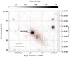 |
Fig. 4. WISE images of UGC 2885 in bands W1 (3.6 μm; grey scale) and W4 (22 μm; contours). The dashed blue circle is the W1 beam size ( |

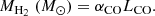
The routine of transforming the original WISE flux units, digital numbers (DNs), into physical units involves the use of Eq. (1), where Fsrc is the flux of the source (in DN), fapcor is the aperture correction factor respective to each band, Ftot is the total flux from the elliptical aperture containing NA number of pixels in the galaxy, and  is a measure of the background level, also in DN, estimated from the neighbouring region around the source annulus.
 (1)
(1)
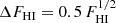
As a final step to obtain the fluxes, we converted DN units into janskys (Jy) using a conversion factor, c:
 (2)
(2)
The WISE explanatory guide also describes the process to derive an error measurement based on an uncertainty map. These images were not available for retrieval, so we decided to use the magnitude-to-standard-deviation ratio for the AllWISE Source Catalog values in order to estimate UGC 2885’s errors in magnitude. This uncertainty approximation relies on the uniformity of the WISE dataset. We calculated the magnitude of each band based on MAG = MAGZP − 2.5log10(Fsrc) – where MAGZP is the magnitude zero-point as determined for each individual band – and the uncertainties as mentioned. We compare these results with the available literature magnitudes in Table 3. Both c and MAGZP were determined from the in-band relative system response curve of the photon count of the WISE telescope, derived from the quantum efficiency of each bandpass (Jarrett et al. 2011).
WISE magnitudes of UGC 2885.
2.3. CO(1–0): IRAM
We are interested in investigating H2 content of UGC 2885 and specifically the cold, less dense, non-star-forming molecular gas. We focused on the ground state rotational transition CO(1−0) (Harris et al. 2010; Emonts et al. 2014). UGC 2885 was observed with the Institut de radioastronomie millimétrique (IRAM) 30 m telescope (Baars et al. 1987) on 2021 1–5 July, 25–30 August, and 14–15 October. A 5′×1.6′ field, with a position angle −47.5 deg, to encompass the entirety of the Hα disc in position switching mode. We acquired the CO(1−0) line with the E0 receiver centred at 109.5 GHz. The data were reduced and mapped using the GILDAS CLASS3 package. We selected the frequency range from 112.29 to 113.59 GHz of the 4 GHz bandwidth, centred around the CO(1−0) line. The bandwidth utilised is about 3000 km s−1. We subtracted a first-order polynomial baseline from each sub-scan before Hanning smoothing and binning the spectra. The resultant maps have  pixels, with a
  FWHM beam, and a spectral resolution of 25 km s−1.
To derive the molecular hydrogen mass, we calculated the CO(1−0) line luminosity from the source flux. We observed that our datacube is significantly affected by noise, background contribution, and edge effects. Thus, we applied a signal masking routine4 from the RADIO-ASTRO-TOOLS code (Ginsburg et al. 2015), which uses Python packages SPECTRAL-CUBE and ASTROPY.MODELLING and is suited to deal with radio data (and its specific units). This method consists of measuring the noise level of the cube based on the pixel-by-pixel standard deviation (σ), as we assumed the noise to be spectrally constant except for a short range of channels where significant signal exists above the mean σ. We applied a sigma-clipping technique to iteratively remove signal from those channels and calculate the average noise level.
Here we defined two signal masks, low and high masks. The low mask represents the signal that is strongly affected by noise (low S/N) and the high mask stands for the signal that is weakly affected by noise (high S/N). The masks are defined by the standard deviation level applied to the regions of the map: a region is described as the 26 pixels that are adjacent to a single pixel in the three dimensions. We used > 2σ and > 5σ for the low signal and high signal masks, respectively. Another adjustable feature is the number of pixels taken in each region that have to surpass both masks. In our case we decided to adopt a conservative criterion to ensure we are able to identify even relatively noisy features (20 pixels for the low signal mask and 3 pixels for the high signal mask). Figure 5 shows the noise model (bottom-left panel) created by the routine as well as the identified signal (bottom-right panel).
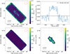 |
Fig. 5. Signal and noise maps derived from the IRAM CO(1−0) datacube. Top left: Peak intensity of the brightness temperature (K) of the original cube. Top right: Noise level (σ) over the spectral range of the cube. The dotted black line represents the average level of noise (σ = 0.0081 K), used to create the following panel. As seen in the central channels, we cannot completely separate the cube’s signal from its noise, even after sigma-clipping. Bottom left: Noise model, or the spatial distribution of noise to be subtracted from the original map. Bottom right: Region with signal that surpasses 5σ. The dashed red circle in the upper-right corner shows the 22.49 arcsec beam size of the IRAM observation. |
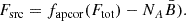
From the output signal map, we derived moment maps that explain the gas dynamics of the system. Moment maps were calculated based on the single Gaussian distribution of the datacube’s spectral range. The zeroth moment (M0), being the integral (or equivalent sum) of the line signal (S(ν)) throughout the spectrum, is defined as the integrated intensity map; in our case, the intensity is in units of K km s−1. The moment-0 map will be used to calculate the CO(1−0) line luminosity. Moments 1 (M1; Eq. (3)) and 2 (M2; Eq. (4)) highlight different aspects of the gas velocity in the galaxy. M1 (shown for completeness but not used in this analysis) measures the centroid velocity of the spectrum peak in each pixel, indicating rotation, while M2 traces the velocity dispersion, or more specifically the square of the emission line width:
 (3)
(3)
 (4)
(4)
Moment maps are displayed in Fig. 6.
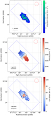 |
Fig. 6. CO moment maps of UGC 2885 from the IRAM datacube. Top: Moment-0 (integrated intensity) map. Middle: Moment-1 (intensity-weighted velocity) map. Bottom: Moment-2 (square root of the intensity-weighted dispersion, or line width) map. The dashed box in all panels highlights the central region. The box is |


2.4. Uncertainties for IRAM datacubes
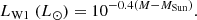
The uncertainties in flux for the radio observations can be estimated based on the line flux emission and line width. We followed the procedure described by Saintonge et al. (2017), with the error in the line flux described in Eq. (5) where Δwch is the spectral channel width (i.e. the channel separation in our datacube, Δwch = 25 km s−1), WCO is the line width (estimated pixel-by-pixel from the Moment-2 map of UGC 2885) and σCO the spectral noise. The spectral noise is calculated from the pixel value histogram of a spectral channel of the datacube. We chose a channel with a high signal-to-noise to fit a skewed Gaussian distribution to the negative half of the data. From Fig. 7, we calculate σCO = 0.0012 K.
 (5)
(5)
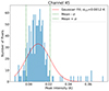 |
Fig. 7. Distribution of the brightness temperature in a channel of the datacube. σCO is the channel standard deviation, here taken as the spectral noise. The dotted green lines are spaced 1σ from the mean value. |
2.5. 21 cm line: WSRT
To understand the evolution of UGC 2885, we also included 21 cm line observations from the WSRT taken in 2004, reported by Hunter et al. (2013) and kindly provided by D. Hunter. For UGC 2885, the images have a spatial resolution of  over a field of 256 × 256 pixels, with each pixel being 4′′. Figure 8 shows the atomic hydrogen distribution compared to the molecular hydrogen in UGC 2885. The blue box was included in this figure to show there is no significant CO(1−0) emission in the outer parts of UGC 2885, pointing to possible star formation activity driven by atomic hydrogen only.
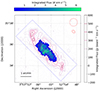 |
Fig. 8. Distribution of H I emission in UGC 2885 from the WSRT data (red contours). Each increment represents 100 Jy beam−1 km s−1. The background filled map is the integrated flux (moment-0) from the IRAM datacube. The blue box is as described in Fig. 6. The dashed red circle is the IRAM beam size, and the solid red ellipse is the WSRT beam size (13 × 19 arcsec). |
3. Estimating the metallicity
By utilising multiple diagnostics, we aimed to gain a comprehensive understanding of the metallicity of UGC 2885. A preliminary examination of spectra can be helpful in choosing metallicity diagnostics: in the UGC 2885 spectra from SITELLE, we observed strong Hα and O II emission, which indicates that UGC 2885 is a high-metallicity galaxy, as expected for its mass (and confirmed in Sect. 6.1). Based on this observation, we chose three different metallicity diagnostics, N2O2, R23, and O3N2, each offering its own advantages and disadvantages (for a review, see Scudder et al. 2021).
3.1. N2O2 index
The N2O2 index uses two spectral lines, N IIλ6584 and O IIλ3727, which are both unaffected by underlying stellar populations (Kewley & Dopita 2002) and expected to be strong even at low signal-to-noise. This index,
![Mathematical equation: $$ \begin{aligned} R = \mathrm{N2O2} = \log \left(\frac{\mathrm{[NII]}\lambda 6584}{\mathrm{[OII]}\lambda 3727}\right), \end{aligned} $$](/articles/aa/full_html/2024/12/aa50916-24/aa50916-24-eq26.gif) (6)
(6)
has well-defined emission lines, lacks local maxima, and is independent of the ionisation parameter (Kewley & Dopita 2002; Paalvast & Brinchmann 2017). It is reported to be reliable for metallicities above half solar (Z > 0.5 Z⊙, log[O/H] + 12 > 8.6; Paalvast & Brinchmann 2017). A disadvantage of this index is that the line ratio is sensitive to dust extinction. However, Kewley & Dopita (2002) found that using the Balmer decrement and a classical reddening curve is sufficient to retrieve a reliable metallicity value. We chose the calibration presented by Kewley & Dopita (2002) to calculate the metallicity with the assumption of 12 + log[O/H]> 8.6,
![Mathematical equation: $$ \begin{aligned} 12 + \log [\mathrm{O/H}] = \log (1.54020 + 1.26602R + 0.167977R^2) + 8.93. \end{aligned} $$](/articles/aa/full_html/2024/12/aa50916-24/aa50916-24-eq27.gif) (7)
(7)
3.2. R23 index
The commonly used R23 strong line ratio, initially introduced by Pagel et al. (1979), makes use of four spectral lines, O IIλ3727, O IIIλ5007, O IIIλ4959 and Hβ. R23 is defined as
![Mathematical equation: $$ \begin{aligned} x = \log \mathrm{R_{23}} = \log \left(\frac{\mathrm{[OII]} \lambda 3727 + \mathrm{[OIII]} \lambda \lambda 4959, 5007}{\mathrm{H}\beta }\right)\cdot \end{aligned} $$](/articles/aa/full_html/2024/12/aa50916-24/aa50916-24-eq28.gif) (8)
(8)
This diagnostic strongly depends on the ionisation parameter and also contains a maximum slightly below the solar value (Kewley & Dopita 2002). R23 is sensitive to abundance but is also double-valued as a function of metallicity, which causes a problem in determining which solution branch best applies (Kewley & Dopita 2002). We used the N2O2 index results, discussed in more detail in Sect. 6.1, to determine that the high-metallicity branch was preferred. We chose the ZKH94 calibration, which is an average of three previous calibrations (Dopita & Evans 1986; McCall et al. 1985; Edmunds & Pagel 1984) and works best in the metal-rich regime, 12 + log[O/H]> 8.35 (Kobulnicky & Kewley 2004):
![Mathematical equation: $$ \begin{aligned} 12 + \log [\mathrm{O/H}] = 9.265 - 0.33x - 0.202x^2 - 0.207x^3 - 0.333x^4. \end{aligned} $$](/articles/aa/full_html/2024/12/aa50916-24/aa50916-24-eq29.gif) (9)
(9)
3.3. O3N2 index
The O3N2 index (Alloin et al. 1979) is a valuable diagnostic for metallicity as its four spectral lines (O IIIλ5007, Hβ, Hα, N IIλ6583) are easily measurable and exhibit minimum wavelength differences between the line pairs, thus minimising the effect of dust reddening (Ho et al. 2015; Paalvast & Brinchmann 2017). O3N2 is defined as
![Mathematical equation: $$ \begin{aligned} \mathrm{O3N2} = \log \left(\frac{\mathrm{[OIII]}\lambda 5007}{\mathrm{H}\beta } \frac{\mathrm{H}\alpha }{\mathrm{[NII]}\lambda 6583}\right). \end{aligned} $$](/articles/aa/full_html/2024/12/aa50916-24/aa50916-24-eq30.gif) (10)
(10)
Paalvast & Brinchmann (2017) found this diagnostic to be sensitive to metallicity in the range 8.12 < 12 + log[O/H]< 9.05, which makes it functional in the high-metallicity regime. As this diagnostic is unaffected by reddening, we chose not to correct the flux maps for reddening. We did not base our results on this metallicity evaluation alone because the ionisation energies for N II and O III are very different; therefore this index is sensitive to changes in energy input from the massive stars (Paalvast & Brinchmann 2017). We used the calibration from Pettini & Pagel (2004):
![Mathematical equation: $$ \begin{aligned} 12 + \log [\mathrm{O/H}] = 8.73-0.32 (\mathrm{O3N2}). \end{aligned} $$](/articles/aa/full_html/2024/12/aa50916-24/aa50916-24-eq31.gif) (11)
(11)
This calibration is useful when −1 < O3N2 < 1.9, and becomes much less reliable beyond O3N2 ≥ 2 (Pettini & Pagel 2004).
3.4. Metallicity uncertainties
The spatially resolved metallicity was estimated by combining line flux maps and their corresponding uncertainty maps in the three different indicators as described in the previous subsections. Metallicities within each of the ellipses described in Sect. 2.1 were computed by averaging the index values over the ellipses. To calculate the metallicity uncertainties, we created uncertainty maps by computing the maximum and minimum values of the relevant line ratios (i.e. (a/b)max = (a + δa)/(b − δb), (a/b)min = (a − δa)/(b + δb)), propagating them through the appropriate definitions (Eqs. (6), (8), and (10)), and then using them to compute the maximum and minimum metallicities (Zmax and Zmin) at each position (Eqs. (7), (9), and (11)). The maximum absolute deviation at each position, max(Zmax − Z, Z − Zmin), was taken as the metallicity uncertainty. Averages of uncertainty maps within each ellipse provided the quoted uncertainty values.
4. Estimating star formation rates
We calculated SFR for UGC 2885 based on WISE mid-infrared W3 and W4 luminosities as described in Eq. (3) of Jarrett et al. (2012) 5. Cluver et al. (2014, 2017) explored the correlation between mid-infrared WISE bands and SFRs while studying nearby galaxy surveys such as GAMA (Hopkins et al. 2013), SINGS (Kennicutt et al. 2003) and KINGFISH (Kennicutt et al. 2011). We applied the relations
 (12)
(12)
and
 (13)
(13)
where WISE luminosities are measured in L⊙ and SFRs in M⊙ yr−1. Cluver et al. (2017) discussed the possible effects of metallicity on the luminosity-SFR relations and found that there is little to no correlation between LW3 and Z. The same effects for LW4 were not addressed. The contaminating effects of the foreground star on W3 and W4 measurements are expected to be smaller than the uncertainties in the SFR calibration.
5. Estimating gas and stellar masses
5.1. Conversion factor αCO
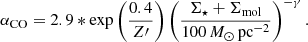
As a final step to calculate the molecular hydrogen mass, we applied a conversion to the CO(1−0) line luminosity. The CO-to-H2 conversion can be found in Sandstrom et al. (2013) and is reproduced here as Eq. (14). The quantity αCO6 is in units of M⊙(K km s−1 pc2)−1 and is determined based on the column density of the molecular gas; LCO is the integrated luminosity of the CO(1−0) line in units of L⊙. In this study we adopted αCO = 4.3, based on the observations of Strong & Mattox (1996) and the application of the model to giant molecular clouds in the Milky Way, explored in detail by Bolatto et al. (2013). Here we assumed the Milky Way’s metallicity and a radially constant value for αCO over the galaxy’s extent:
 (14)
(14)
Applying this factor has some implications for UGC 2885’s molecular properties. The conversion between CO emission and molecular hydrogen mass is thought to depend on metallicity and to also have a radial dependence (Arimoto et al. 1996). As metallicity increases, αCO decreases, since by definition there is a lower hydrogen abundance in relation to oxygen (Hirashita 2023; Sandstrom et al. 2024). We discuss the effects of the estimated metallicities of this study in calculating MH2 for UGC 2885 in Sect. 6.3.
5.2. Neutral hydrogen mass
The H I mass is calculated based on Eq. (15) where FHI is the integrated flux of the H I line, in units of Jy km s−1. We estimated the uncertainties for the H I mass based on the relations described by Doyle & Drinkwater (2006), shown in Eqs. (16) and (17):
 (15)
(15)
 (16)
(16)
 (17)
(17)
5.3. Stellar mass-to-light ratio
To compute the stellar mass (M*), we followed the procedure described by Parkash et al. (2018). This relation, shown in Eq. (18), uses the W1 in-band luminosity with MSun = 3.24 (Jarrett et al. 2012) and M as the absolute magnitude of the WISE 1 band:
 (18)
(18)
The mass-to-light ratio (Υ⋆ = M*/L) of a galaxy depends on various properties of the object, such as its morphology and colour. Multiple studies have explored the different equivalences between emitted light and stellar content using WISE colours (most notably W1–W2 and W1–W3; Jarrett et al. 2012; Meidt et al. 2014; Kettlety et al. 2018; Parkash et al. 2018). Here we adopted M*/LW1 = 0.35 ± 0.11 M⊙/L⊙ as Jarrett et al. (2023) find a tight linear relation between stellar mass and W1 luminosity.
6. Results and discussion
6.1. Metallicity and metallicity gradient
Using N2O2, R23, and O3N2, the global metallicity was calculated within a radius of 25 kpc to be Z = 9.28, 9.08 and 8.74, with uncertainties of 0.17 dex, 0.07 dex, and 0.16 dex, respectively. All three global metallicities show that UGC 2885 is in the high-metallicity regime, consistent with our expectations based on the mass-metallicity relationship. The N2O2 and R23 measurements agree within their uncertainties, while the O3N2 value is slightly lower; possible explanations include the greater sensitivity of O3N2 to variations in the input ionising spectrum, or the true metallicity of the galaxy being above the validity range of this indicator (see Sect. 3.3). We further assessed the metallicity across three distinct zones within UGC 2885’s disc to determine its metallicity gradient, as illustrated in Fig. 9. (As the measured metallicities are well above the lower limit for which the calibrations are valid, we do not expect our original assumption of high metallicity to affect measurements of the metallicity gradient). Within the uncertainties, none of the three indicators shows a strong metallicity gradient. Table 4 gives the metallicities and gradients determined with N2O2, R23, and O3N2 diagnostics.
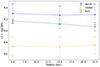 |
Fig. 9. Metallicity calculated using N2O2, R23, and O3N2 diagnostics. The specific radial zones evaluated were 0–10 kpc (ellipse A), 10–20 kpc (ellipse B), and 20–25 kpc (ellipse C). The overall metallicity values calculated with N2O2 and R23 agree well, with the O3N2 metallicity offset to a lower value. None of the three indicators shows a strong metallicity gradient. |
Metallicity gradient observed in UGC 2885.
Local galaxies often exhibit negative metallicity gradients, with typical values from 0 to −0.1 dex kpc−1 (Sharda et al. 2021). The negative pattern arises as star formation in galaxies often starts at the core and expands outwards. Consequently, the central region tends to be more metal-rich compared to its outskirts. Isolated galaxies that do not undergo mergers tend to evolve smoothly; this allows steady star formation, resulting in enrichment, and creates a shallower metallicity gradient (Tissera et al. 2021). Our prediction for an isolated galaxy of this stellar mass would be a shallow negative or flat metallicity gradient accompanied by high average metallicity (Mannucci et al. 2010), and our observations are consistent with this prediction.
6.2. Star formation rate
The SFR was estimated from Eqs. (12) and (13), respectively, as 1.41 ± 0.72 M⊙ yr−1 and 1.86 ± 1.24 M⊙ yr−1, for a mean value of 1.63 ± 0.72 M⊙ yr−1. This agrees with the calculated 2.47 M⊙ yr−1 of Hunter et al. (2013) within the uncertainties of this work and assuming a similar uncertainty value attributed to their measurement. However, Hunter et al. (2013) used a different estimated distance for UGC 2885, DL = 79.10 Mpc. If those authors had used DL = 84.34 Mpc their SFR would increase to 2.80 M⊙ yr−1. The divergence could be attributed to the star formation indicators used: Hα emission probes star formation on shorter timescales than ultraviolet or infrared emission (Kennicutt & Evans 2012).
Considering UGC 2885’s size, we are also interested in calculating its SFR surface density (ΣSFR). In this work the surface densities are estimated at the outer radius of the largest ellipse in Fig. 3, 25 kpc. ΣSFR is calculated as 1.97 × 10⁻³ M⊙ yr−1 kpc−2 and is comparable to other giant galaxies in the nearby Universe, ranging from 0.50−2.16 × 10⁻³ M⊙ yr−1 kpc−2 (Ray et al. 2024). This result is surprising considering that Ray et al. (2024) used spatially resolved measurements of SFR, which is the main caveat of this comparison.
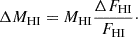
6.3. Molecular hydrogen mass and star formation efficiency
We find a molecular hydrogen mass of  . This represents the first estimate of the H2 content of UGC 2885 and allowed us to calculate the star formation efficiency (SFE) of this galaxy. We derived the SFE from the relation SFE (yr−1) = SFR/MH2, finding it to have a mean value of 8.67 ± 4.20 × 10⁻¹² yr−1 using the mean calculated SFR from Sect. 6.2. Nearby disc galaxies of high mass (
 ) have a total molecular gas mass that ranges from ∼108 to
  , indicating that UGC 2885 is an unique object with a large gas reservoir (Saintonge et al. 2017). Moreover, nearby discs have a mean SFE of 5.25 ± 2.50 × 10⁻¹⁰ yr−1 (Leroy et al. 2008), which makes UGC 2885 extremely inefficient in forming stars from its available molecular gas. Our dataset could be used to estimate an upper limit on the integrated intensity of the CO(1−0) line in areas without a positive detection, with the 3σ upper limit being 0.12 K km s−1 beam−1.
We also studied the effect of correcting the conversion factor αCO for metallicity on the estimation of MH2. Bolatto et al. (2013) presented a way to calculate the αCO that is dependent on both the galaxy’s metallicity and the total surface density. This relation is shown in Eq. (19)7. Here we used Z′ as the metallicity scaled by the solar metallicity (Z′=0.014 or 12 + log(O/H = 8.7); Asplund et al. 2009). The Σ⋆ and Σmol are the surface densities of the stellar and molecular hydrogen masses, respectively. If the sum of these two values is ≥100 M⊙ pc−2, then γ = 0.5; otherwise, γ = 0.
 (19)
(19)
The sum Σ⋆ + Σmol is calculated as 8.10 × 10⁵ M⊙ pc−2 – details on the stellar mass calculation are discussed below in Sect. 6.5. We estimated a αCO of 2.91 for all metallicity indices presented in this work. Using this conversion factor, we calculated the molecular gas mass as MH2 = 1.26 ± 0.16 × 10¹¹ M⊙. In this work, we utilised the uncorrected molecular gas mass value, as our primary focus is on comparing this measurement to other studies, some of which do not implement the same corrections. The primary study we compare our results with in Sect. 6.6 applies a correction based on a property we directly investigate.
6.4. Neutral hydrogen mass
The atomic hydrogen mass of UGC 2885 is calculated to be MHI = 3.73 ± 0.38 × 10¹⁰ M⊙. This value can be compared to the one found in Hunter et al. (2013),  . If this mass was measured using DL = 84.34 Mpc, the previous authors would have obtained
  . MHI remains consistent between our calculations and the available estimate.
6.5. Stellar mass
We estimate UGC 2885’s stellar mass as  . Di Teodoro et al. (2023) calculated the same property as
  using DL = 71 Mpc. M⋆ does not agree within the uncertainties with the most recent published value. Although Di Teodoro et al. (2023) used the same available WISE images to estimate stellar mass, they chose a larger mass-to-light ratio than ours (Υ⋆ = 0.6), which could be the reason for this divergence. If those authors had applied our value of DL = 84.34 Mpc and a Υ⋆ = 0.35 ± 0.11 M⊙/L⊙, they would have estimated
  , which is even more discrepant. The fixed mass-to-light ratio used by Di Teodoro et al. (2023) might be more appropriate for elliptical or spheroidal galaxies with little star formation (Meidt et al. 2014). The Υ⋆ used in this work also takes into account the WISE colours, which are reflective of star-forming processes such as warm dust in the interstellar medium (Leroy et al. 2019).
6.6. UGC 2885’s position on the star-forming main sequence of galaxies
We explore the relationship between the SFR, H2 mass, H I mass, and stellar mass for UGC 2885. Studies with simulated or observed galaxies have shown a strong correlation between stellar mass and SFR in nearby galaxies, the so-called star-forming main sequence (SFMS; Brinchmann et al. 2004). The xCOLD GASS survey explored the SFR–M⋆ plane for local galaxies with available IRAM 30m observations (Saintonge et al. 2017). Our comparison to their sample would place UGC 2885 along the distribution but at the higher end of stellar mass (see Figs. 7 and 8 of Saintonge et al. 2017). This prediction is reasonable as we expect a flattening of the SFR with a decrease in the available gas reservoir. Those authors also discuss the gas depletion time for their sample of galaxies. Gas depletion time is defined as the time it takes for the gas to be consumed (by either being transformed into stars or accreted by the central black hole) and can be estimated as tdep = 1/SFE for both molecular and atomic hydrogen gas. For UGC 2885, the depletion times are tdep (H2) = 1.15 ± 0.51 × 10¹¹ yr and tdep (HI) = 2.29 ± 1.04 × 10¹⁰ yr. Figure 10 shows the SFR–M⋆ plane for the xCOLD GASS sample colour-coded by the depletion times, as well as the position of UGC 2885 on it.
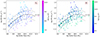 |
Fig. 10. SFMS of the xCOLD GASS sample with available ALFALFA H I fluxes. The solid line is the SFMS, and the dashed lines show ±0.4 dex scatter as described by Saintonge et al. (2017). Colour represents the depletion time (tdep) of the molecular gas (left panel) and atomic gas (right panel). |
Compared to super-spiral galaxies, UGC 2885 sits far above the representative curve due to its high molecular-to-stellar mass ratio (log fH2 = MH2/M⋆ = −0.41 ± 0.33). fH2 for UGC 2885 deviates from higher mass objects (log M⋆ > 10.47 M⊙), as their molecular-to-stellar mass ratio tends to be much lower (mean value of log fH2 = −1.36 ± 0.02; Lisenfeld et al. 2023). Figure 11 shows the representative curve of the SFR–M⋆ plane for super spirals compared to UGC 2885.
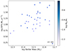 |
Fig. 11. SFR as a function of stellar mass for a sample of massive disc galaxies (Lisenfeld et al. 2023) colour-coded by their molecular-to-stellar mass ratio (MH2/M⋆). UGC 2885 is displayed for comparison but was not included in the fitting of the SFR–M⋆ plane. The range of stellar masses differs from that of Fig. 10, as super-spiral galaxies have logM⋆ > 10.47 M⊙. |
6.7. Fundamental metallicity relation
The fundamental metallicity relation (FMR) relates stellar mass, gas-phase metallicity (Z), and SFR (Mannucci et al. 2010). Despite its immense size, high metallicity, and low SFR for a massive galaxy, UGC 2885 remains consistent with the FMR. Figure 12 is the FMR recreated using data provided in Table 1 of Mannucci et al. (2010), where the values within the bins are the median metallicity found at each given SFR and M⋆. Using the previously published stellar mass and star formation for UGC 2885 (logM⋆ = 11.2 M⊙, logSFR = 0.4 M⊙ yr−1; Di Teodoro et al. 2023; Hunter et al. 2013), the FMR presented in Fig. 12 predicts a metallicity of Z ≈ 9.06. The arrow in Fig. 12 indicates our larger estimated stellar mass and SFR values(log M⋆ = 11.68 M⊙, logSFR = 0.48 M⊙ yr−1) from which the FMR predicts a metallicity of Z ≈ 9.08. Both predicted metallicity values are consistent with the global values calculated from our data; within the uncertainties of our measurements, we find that UGC 2885 is not an outlier to the FMR.
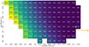 |
Fig. 12. Relation between the galaxy stellar mass, SFR, and metallicity based on the data from Mannucci et al. (2010). The orange star represents UGC 2885’s position in the chart based on our calculated values: stellar mass log(M⋆)=11.68 and SFR log(SFR)=0.48. The blue star represents UGC 2885’s position in the chart based on previous values (log(M⋆)=11.3, log(SFR)=0.40; Hunter et al. 2013). Both metallicities found using the FMR are comparable to the results found using the emission line diagnostics to calculate metallicity (Z ≈ 9). |
Mannucci et al. (2010) found that at large stellar masses (log M⋆ > 10.9), there is a lack of correlation between stellar mass and metallicity. At low SFRs, the correlation also weakens. This is due to the fact that there is a turnover mass ( ) where metallicity begins to saturate. As the metallicity saturates, the mass-metallicity relation also begins to flatten (Zahid et al. 2014).
6.8. The evolution of UGC 2885
The distance between a galaxy and the SFMS (ΔMS) is an important proxy for galaxy evolutionary stage at the time of observations. Quiescent galaxies, that is, galaxies with dormant star formation, are generally found to be distant from the MS, specifically below the trend. These galaxies will most likely continue to form stars at a constant but low rate, meaning their global metallicity ceases to change significantly (Looser et al. 2024).
We expect galaxies to increase their metallicity after cycles of star formation and stellar mass growth. Therefore, UGC 2885’s high metallicity indicates that the galaxy has cycled through many phases of star formation. This could explain UGC 2885’s location in relation to the SFMS, as we see that ΔMS is inversely proportional to Z (Peng et al. 2015) considering that the galaxy will use its gas reservoir to increase its stellar mass, consequently increasing metallicity. The molecular gas fraction fH2 is also a main factor to determine ΔMS since a galaxy will only be star-forming with an available gas reservoir. Here we observe a strong discrepancy with the starvation hypothesis as high-metallicity, non-star-forming galaxies are found to have lower gas fractions than those of MS galaxies. From our measurements, UGC 2885 has a fH2 that is comparable to galaxies above the main sequence (Saintonge et al. 2017). Its molecular gas mass is about three times the maximum MH2 of local post-starburst galaxies with comparable SFRs (see Fig. 3 of French 2021), suggesting that UGC 2885 did not deplete its gas reservoir in a recent starburst.
The issue with using the SFMS as a probe for galaxy evolution therefore lies in the fact that it does not take a galaxy’s gas fraction into account. More fundamental relations can be used instead, such as the molecular gas main sequence (Lin et al. 2019). Based on this relation, molecular hydrogen content and stellar mass will follow a linear trend for star-forming galaxies. The strong linearity of the MH2 − M⋆ plane comes from the gravitational potential caused by either the dark matter content dominance in the galaxy or the baryonic components dominating instead. In both cases, the gas fraction will not affect the trend for low redshifts (Baker et al. 2023; Lin et al. 2019). Figure 13 shows that this might not be the case for UGC 2885 as its current star formation is insufficient to place the galaxy along the linear relation when comparing to galaxies with a high molecular gas reservoir.
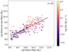 |
Fig. 13. Molecular hydrogen mass as a function of stellar mass (molecular gas main sequence) for the xCOLD GASS sample. The sample is colour-coded by SFR. UGC 2885 is far above the relation due to its large gas reservoir. |
6.9. Could a galactic bar quench UGC 2885’s star formation?
Saintonge et al. (2016) discussed the SFMS at the higher end of stellar masses. Specifically, galaxies with M* > 1010.8 M⊙ might be part of a ‘danger zone’ (at risk of becoming red and dead). Their vast molecular gas reservoir is not being transformed into stars by some sort of quenching mechanism within the last 1 Gyr. These objects have a high molecular-to-atomic gas ratio, and it is thought that these galaxies have a mechanism that moves gas towards the central region. Saintonge et al. (2016) also observe that the majority of the galaxies in the danger zone have strong galactic bars that are potentially strong drivers of gas across the host and towards its centre. We notice that the distribution of molecular gas in UGC 2885 does not expand isotropically from the galactic centre. This is expected for galaxies with galactic bars as seen in the EMPIRE survey (e.g. NGC 2903, NGC 3627, and NGC 6946, Jiménez-Donaire et al. 2019). High-resolution measurements of the molecular hydrogen of UGC 2885 could shed light on its radial distribution, helping confirm this hypothesis.
It is known that turbulent velocity fields are drivers of shocks in the interstellar medium (Hopkins et al. 2012). This mechanism can constrain star formation activity on small scales due to its random motion nature, which counteracts self-gravity. Galactic bars induce gravitational torques due to the bar potential – perpendicular to the structure – which then causes a decrease in the gas rotational motion, meaning an increase in local turbulence. Consequently, the randomness of the gas can be traced by observing the molecular gas dispersion (Kim & Ostriker 2007).
Figure 6 (bottom panel) shows the velocity dispersion of the molecular gas for UGC 2885. A box around the central region of the galaxy highlights where the higher dispersion correlates with the presence of H2 gas (see the top panel of Fig. 6). We consider this to be tentative evidence of a molecular bar. From previous observations, UGC 2885 has not been reported to be a barred galaxy, and a preliminary analysis of the HST/WFC3 F814W images does not appear to show a stellar bar.
Galaxy metallicity is typically affected by star formation, inflows and outflows in the circumgalactic environment. A bar within the galaxy may contribute to the inflow and outflow processes. UGC 2885, being an isolated galaxy, is unlikely to be significantly affected by external inflow processes. The AGN suggested by Holwerda et al. (2021) may contribute to the outflow. It is uncertain how heavily AGN outflow affects the metallicity and star formation within the galaxy, as it is still unclear how the AGN is fuelled.
Galaxies with strong bars usually have high metallicity values. Bars facilitate outer-disc to inner-disc inflow potential, which means that barred galaxies can process gas into stars more rapidly, thus increasing the central metallicity (Vera et al. 2016). Another possible effect of a bar on the galactic metallicity is the shape of the metallicity gradient. Chen et al. (2023) show that barred galaxies can flatten the radial metallicity profile. We observe this flattening for UGC 2885 in Fig. 9. Therefore, we conjecture that the presence of a molecular gas bar could explain some of the properties observed. Since this structure is not noticed in any other wavebands, we propose that its composition is mainly molecular and newly acquired by UGC 2885. Stronger evidence is needed to confirm this hypothesis, such as high-resolution sub-millimetre observations.
7. Conclusions
We present a multi-wavelength imaging analysis of UGC 2885, an extreme spiral in the nearby Universe with remarkably ordinary properties aside from its high molecular gas content. UGC 2885 has a typical brightness disc with signs of star formation along its arms, as well as a relatively low central activity. We used both archival and new data over a wide range of wavelengths to provide an overview of several properties of this galaxy. Our findings are summarized as:
-
1.
We used strong emission lines observed in SITELLE datacubes to calculate three different metallicity indicators (N2O2, R23, and O3N2). The global metallicity is Z ≈ 9.0 ± 0.13, which places UGC 2885 in the high-metallicity regime and is consistent with its high stellar mass.
-
2.
There is little evidence of a strong metallicity gradient in UGC 2885 in any of the three metallicity indicators. Figure 9 shows that the metallicity is uniform within ±0.3 dex over a large radial extent in this galaxy.
-
3.
UGC 2885 aligns with the FMR. This indicates, based on its stellar mass and SFR, a metallicity of Z ≈ 9.06.
-
4.
We find a mean global SFR of 1.63 ± 0.72 M⊙ yr−1 derived from WISE W3 and W4 imaging. This is comparable to the only available calculated SFR in the literature for this object (SFR = 2.47 M⊙ yr−1; Hunter et al. 2013) assuming the same uncertainty range for their result. This is a low SFR compared to those of super-spiral galaxies (5 − 65 M⊙ yr−1), objects that are generally positioned above the main sequence of star-forming galaxies in the nearby Universe.
-
5.
The integrated molecular hydrogen mass (MH2) is calculated to be 1.89 ± 0.24 × 10¹¹ M⊙. Galaxies at the higher end of the stellar mass range generally have much lower H2 masses, as we expect the molecular gas to be consumed over the galaxy’s lifetime by star formation, black hole accretion, or external processes. This indicates that UGC 2885 is undergoing a quenching event, which is supported by its high depletion times based on both the molecular (tdep (H2) = 1.15 ± 0.51 × 10¹¹ yr) and neutral hydrogen (tdep (HI) = 2.29 ± 1.04 × 10¹⁰ yr) content.
-
6.
A high tdep is characteristic of galaxies below the SFMS. Although UGC 2885 is located at the higher end of the distributions for stellar mass, its actual position in relation to other massive galaxies changes dramatically when we include the relationship between the SFR and molecular mass. The position of galaxies on the main sequence is thus determined by a combination of factors – mainly the molecular gas fraction and the SFE (Saintonge et al. 2016) – as seen in Figs. 10 and 11.
-
7.
UGC 2885 has an extreme molecular-to-stellar mass ratio (fH2 = −0.41 ± 0.33). We do not know how cold gas could have been added to this galaxy as it is completely isolated, without companions or a clear recent merging event.
-
8.
We suggest that UGC 2885 contains a barred structure formed mainly of molecular mass The moment-0 and moment-2 maps show that UGC 2885’s molecular mass is located in its central region, with disturbed kinematics. This is the first study of the H2 gas of UGC 2885, which could explain why no other previous work on this galaxy has suggested the existence of a bar. The bar mechanisms that control the gas dynamics – specifically inflows – within the central regions of galaxies are potential drivers of star formation quenching and high metallicity, consistent with the observations in this study.
We conclude that UGC 2885 has produced stars through many cycles of star formation and has undergone no significant recent starburst or merging events. These factors might be responsible for the galaxy’s current stage of evolution in terms of stellar content, population (metallicity), and SFR. The processes that fuel the large molecular gas reservoir remain uncertain. Possible directions for future work include a spatially resolved analysis of the star formation, gas content, gas and stellar kinematics, and morphological decomposition aimed at learning more about the galaxy’s structure at all radii, from the putative bar to the spiral arms. Such an analysis would benefit from molecular gas and dust maps at higher spatial resolution than what is currently available.
When literature measurements are quoted without uncertainties, no uncertainty values were given in the previous work.
Grenoble Image and Line Data Analysis Software Continuum and Line Analysis Single-dish Software, http://www.iram.fr/IRAMFR/GILDAS
Lband is the ‘in-band’ luminosity, defined by Lband(L⊙)=10−0.4(M(band)−M⊙(band)).
Also denoted as XCO in units of cm−2 (K km s−1)−1.
This is a modified version that avoids incongruous αCO values in low-surface-density regions (Sun et al. 2023).
Acknowledgments
The authors thank the anonymous referee for a helpful report. We thank Dr. C. Rhea for helpful discussions and guidance in the use of LUCI, Dr. D. Hunter for kindly providing the WSRT 21-cm line observations, C. Robertson for helpful comments on the galaxy’s spectra, and H. Christie for assistance with Figure 1. Based on observations obtained with SITELLE, a joint project between Université Laval, ABB-Bomem, Université de Montréal, and the Canada-France-Hawaii Telescope (CFHT) with funding support from the Canada Foundation for Innovation (CFI), the National Sciences and Engineering Research Council of Canada (NSERC), Fond de Recherche du Quebec – Nature et Technologies (FRQNT) and CFHT. The Canada-France-Hawaii Telescope is operated from the summit of Maunakea by the National Research Council of Canada, the Institut National des Sciences de l’Univers of the Centre National de la Recherche Scientifique of France, and the University of Hawaii. The observations at the Canada-France-Hawaii Telescope were performed with care and respect from the summit of Maunakea which is a significant cultural and historic site. This work is based on observations carried out under project number 076-21 with the IRAM 30m telescope. IRAM is supported by INSU/CNRS (France), MPG (Germany) and IGN (Spain). This research is based on observations made with the NASA/ESA Hubble Space Telescope obtained from the Space Telescope Science Institute, which is operated by the Association of Universities for Research in Astronomy, Inc., under NASA contract NAS 5-26555. These observations are associated with program(s), GO-15107 (PI B. W. Holwerda). P. B. acknowledges support from a Natural Sciences and Engineering Research Council of Canada Discovery Grant. S. K. gratefully acknowledges funding from the European Research Council (ERC) under the European Union’s Horizon 2020 research and innovation programme (grant agreement No. 789410).
References
- Alloin, D., Collin-Souffrin, S., Joly, M., & Vigroux, L. 1979, A&A, 78, 200 [Google Scholar]
- Arimoto, N., Sofue, Y., & Tsujimoto, T. 1996, PASJ, 48, 275 [Google Scholar]
- Asplund, M., Grevesse, N., Sauval, A. J., & Scott, P. 2009, ARA&A, 47, 481 [NASA ADS] [CrossRef] [Google Scholar]
- Baars, J., Hooghoudt, B., Mezger, P., & de Jonge, M. 1987, A&A, 175, 319 [NASA ADS] [Google Scholar]
- Baker, W. M., Maiolino, R., Belfiore, F., et al. 2023, MNRAS, 518, 4767 [Google Scholar]
- Barbary, K. 2016, https://doi.org/10.5281/zenodo.168220 [Google Scholar]
- Bolatto, A. D., Wolfire, M., & Leroy, A. K. 2013, ARA&A, 51, 207 [CrossRef] [Google Scholar]
- Brinchmann, J., Charlot, S., White, S. D., et al. 2004, MNRAS, 351, 1151 [NASA ADS] [CrossRef] [Google Scholar]
- Brown, M. J. I., Jarrett, T., & Cluver, M. E. 2014, PASA, 31, e049 [NASA ADS] [CrossRef] [Google Scholar]
- Brown, M. J., Moustakas, J., Kennicutt, R. C., et al. 2017, ApJ, 847, 136 [NASA ADS] [CrossRef] [Google Scholar]
- Canzian, B., Allen, R., & Tilanus, R. 1993, ApJ, 406, 457 [NASA ADS] [CrossRef] [Google Scholar]
- Cardelli, J. A., Clayton, G. C., & Mathis, J. S. 1989, ApJ, 345, 245 [Google Scholar]
- Chen, Q.-H., Grasha, K., Battisti, A. J., et al. 2023, MNRAS, 519, 4801 [NASA ADS] [CrossRef] [Google Scholar]
- Chiang, Y.-K. 2023, ApJ, 958, 118 [NASA ADS] [CrossRef] [Google Scholar]
- Cluver, M. E., Jarrett, T. H., Hopkins, A. M., et al. 2014, ApJ, 782, 90 [Google Scholar]
- Cluver, M., Jarrett, T. H., Dale, D., et al. 2017, ApJ, 850, 68 [NASA ADS] [CrossRef] [Google Scholar]
- Cutri, R., Wright, E., Conrow, T., et al. 2012, Explanatory Supplement to the WISE All-Sky Data Release Products, 1 [Google Scholar]
- Cutri, R. E., Wright, E., Conrow, T., et al. 2021, VizieR Online Data Catalog: II/328 [Google Scholar]
- De Vaucouleurs, G., de Vaucouleurs, A., Harold, G., et al. 2013, Third Reference Catalogue of Bright Galaxies: Volume III (New York: Springer) [Google Scholar]
- Di Teodoro, E. M., Posti, L., Fall, S. M., et al. 2023, MNRAS, 518, 6340 [Google Scholar]
- Dietrich, J., Weiner, A. S., Ashby, M. L., et al. 2018, MNRAS, 480, 3562 [NASA ADS] [CrossRef] [Google Scholar]
- Dopita, M. A., & Evans, I. N. 1986, ApJ, 307, 431 [NASA ADS] [CrossRef] [Google Scholar]
- Doyle, M. T., & Drinkwater, M. J. 2006, MNRAS, 372, 977 [Google Scholar]
- Drissen, L., Martin, T., Rousseau-Nepton, L., et al. 2019, MNRAS, 485, 3930 [NASA ADS] [CrossRef] [Google Scholar]
- Du, W., Cheng, C., Du, P., Du, L., & Wu, H. 2023, ApJ, 959, 105 [NASA ADS] [CrossRef] [Google Scholar]
- Edmunds, M. G., & Pagel, B. E. J. 1984, MNRAS, 211, 507 [NASA ADS] [CrossRef] [Google Scholar]
- Emonts, B., Norris, R. P., Feain, I., et al. 2014, MNRAS, 438, 2898 [NASA ADS] [CrossRef] [Google Scholar]
- Falco, E. E., Kurtz, M. J., Geller, M. J., et al. 1999, PASP, 111, 438 [Google Scholar]
- Fitzpatrick, E., & Massa, D. 2007, ApJ, 663, 320 [NASA ADS] [CrossRef] [Google Scholar]
- French, K. D. 2021, PASP, 133, 072001 [NASA ADS] [CrossRef] [Google Scholar]
- Gao, F., Wang, L., Pearson, W., et al. 2020, A&A, 637, A94 [NASA ADS] [CrossRef] [EDP Sciences] [Google Scholar]
- Ginsburg, A., Robitaille, T., Beaumont, C., et al. 2015, ASP Conf. Ser., 499, 363 [NASA ADS] [Google Scholar]
- Harris, A., Baker, A., Zonak, S., et al. 2010, ApJ, 723, 1139 [NASA ADS] [CrossRef] [Google Scholar]
- Hill, G. J., MacQueen, P. J., & Smith, M. P. 2008, SPIE Conf. Ser., 7014, 701470 [NASA ADS] [Google Scholar]
- Hirashita, H. 2023, MNRAS, 522, 4612 [NASA ADS] [CrossRef] [Google Scholar]
- Ho, I. T., Kudritzki, R.-P., Kewley, L. J., et al. 2015, MNRAS, 448, 2030 [NASA ADS] [CrossRef] [Google Scholar]
- Holwerda, B. W., Wu, J. F., Keel, W. C., et al. 2021, ApJ, 914, 142 [NASA ADS] [CrossRef] [Google Scholar]
- Hopkins, P. F., Quataert, E., & Murray, N. 2012, MNRAS, 421, 3488 [NASA ADS] [CrossRef] [Google Scholar]
- Hopkins, A. M., Driver, S. P., Brough, S., et al. 2013, MNRAS, 430, 2047 [NASA ADS] [CrossRef] [Google Scholar]
- Hunter, D. A., Elmegreen, B. G., Rubin, V. C., et al. 2013, AJ, 146, 92 [NASA ADS] [CrossRef] [Google Scholar]
- Jarrett, T., Cohen, M., Masci, F., et al. 2011, ApJ, 735, 112 [NASA ADS] [CrossRef] [Google Scholar]
- Jarrett, T., Masci, F., Tsai, C., et al. 2012, AJ, 145, 6 [Google Scholar]
- Jarrett, T. H., Cluver, M. E., Taylor, E. N., et al. 2023, ApJ, 946, 95 [NASA ADS] [CrossRef] [Google Scholar]
- Jiménez-Donaire, M. J., Bigiel, F., Leroy, A., et al. 2019, ApJ, 880, 127 [CrossRef] [Google Scholar]
- Joye, W. A., & Mandel, E. 2003, ASP Conf. Ser., 295, 489 [Google Scholar]
- Kennicutt, R. C., & Evans, N. J. 2012, ARA&A, 50, 531 [NASA ADS] [CrossRef] [Google Scholar]
- Kennicutt, R. C., Armus, L., Bendo, G., et al. 2003, PASP, 115, 928 [NASA ADS] [CrossRef] [Google Scholar]
- Kennicutt, R., Calzetti, D., Aniano, G., et al. 2011, PASP, 123, 1347 [NASA ADS] [CrossRef] [Google Scholar]
- Kereš, D., Katz, N., Weinberg, D. H., & Davé, R. 2005, MNRAS, 363, 2 [Google Scholar]
- Kettlety, T., Hesling, J., Phillipps, S., et al. 2018, MNRAS, 473, 776 [NASA ADS] [CrossRef] [Google Scholar]
- Kewley, L. J., & Dopita, M. A. 2002, ApJS, 142, 35 [Google Scholar]
- Kewley, L. J., Groves, B., Kauffmann, G., & Heckman, T. 2006, MNRAS, 372, 961 [Google Scholar]
- Kim, W.-T., & Ostriker, E. C. 2007, ApJ, 660, 1232 [NASA ADS] [CrossRef] [Google Scholar]
- Kobulnicky, H. A., & Kewley, L. J. 2004, ApJ, 617, 240 [CrossRef] [Google Scholar]
- Lacey, C., & Cole, S. 1993, MNRAS, 262, 627 [NASA ADS] [CrossRef] [Google Scholar]
- Leroy, A. K., Walter, F., Brinks, E., et al. 2008, AJ, 136, 2782 [Google Scholar]
- Leroy, A. K., Sandstrom, K. M., Lang, D., et al. 2019, ApJS, 244, 24 [Google Scholar]
- Lewis, B. 1985, ApJ, 292, 451 [NASA ADS] [CrossRef] [Google Scholar]
- Lin, L., Pan, H.-A., Ellison, S. L., et al. 2019, ApJ, 884, L33 [NASA ADS] [CrossRef] [Google Scholar]
- Lisenfeld, U., Ogle, P. M., Appleton, P. N., Jarrett, T. H., & Moncada-Cuadri, B. M. 2023, A&A, 673, A87 [NASA ADS] [CrossRef] [EDP Sciences] [Google Scholar]
- Looser, T. J., D’Eugenio, F., Piotrowska, J. M., et al. 2024, MNRAS, 532, 2832 [NASA ADS] [CrossRef] [Google Scholar]
- Mannucci, F., Cresci, G., Maiolino, R., Marconi, A., & Gnerucci, A. 2010, MNRAS, 408, 2115 [NASA ADS] [CrossRef] [Google Scholar]
- Martin, T., Drissen, L., & Joncas, G. 2012, SPIE Conf. Ser., 8451, 84513K [NASA ADS] [Google Scholar]
- McCall, M. L., Rybski, P. M., & Shields, G. A. 1985, ApJS, 57, 1 [CrossRef] [Google Scholar]
- Meidt, S. E., Schinnerer, E., Van de Ven, G., et al. 2014, ApJ, 788, 144 [NASA ADS] [CrossRef] [Google Scholar]
- Moustakas, J., Lang, D., Dey, A., et al. 2023, ApJS, 269, 3 [NASA ADS] [CrossRef] [Google Scholar]
- Ogle, P. M., Lanz, L., Nader, C., & Helou, G. 2016, ApJ, 817, 109 [NASA ADS] [CrossRef] [Google Scholar]
- Paalvast, M., & Brinchmann, J. 2017, MNRAS, 470, 1612 [CrossRef] [Google Scholar]
- Pagel, B. E. J., Edmunds, M. G., Blackwell, D. E., Chun, M. S., & Smith, G. 1979, MNRAS, 189, 95 [NASA ADS] [CrossRef] [Google Scholar]
- Parkash, V., Brown, M. J., Jarrett, T., & Bonne, N. J. 2018, ApJ, 864, 40 [NASA ADS] [CrossRef] [Google Scholar]
- Peng, Y., Maiolino, R., & Cochrane, R. 2015, Nature, 521, 192 [Google Scholar]
- Pettini, M., & Pagel, B. E. J. 2004, MNRAS, 348, L59 [NASA ADS] [CrossRef] [Google Scholar]
- Ray, S., Dhiwar, S., Bagchi, J., & Pandge, M. 2024, MNRAS, 527, 9999 [Google Scholar]
- Rhea, C. L., Rousseau-Nepton, L., Covington, J., et al. 2021a, https://doi.org/10.5281/zenodo.5385351 [Google Scholar]
- Rhea, C., Hlavacek-Larrondo, J., Rousseau-Nepton, L., Vigneron, B., & Guité, L.-S. 2021b, Res. Notes AAS, 5, 208 [NASA ADS] [CrossRef] [Google Scholar]
- Roelfsema, P., & Allen, R. 1985, A&A, 146, 213 [NASA ADS] [Google Scholar]
- Romanishin, W. 1983, MNRAS, 204, 909 [NASA ADS] [CrossRef] [Google Scholar]
- Rubin, V. C., Ford, W. K., & Thonnard, N. 1980, ApJ, 238, 471 [NASA ADS] [CrossRef] [Google Scholar]
- Saburova, A. S., Chilingarian, I. V., Kasparova, A. V., et al. 2021, MNRAS, 503, 830 [NASA ADS] [CrossRef] [Google Scholar]
- Saintonge, A., Catinella, B., Cortese, L., et al. 2016, MNRAS, 462, 1749 [Google Scholar]
- Saintonge, A., Catinella, B., Tacconi, L. J., et al. 2017, ApJS, 233, 22 [Google Scholar]
- Salim, S., Lee, J. C., Janowiecki, S., et al. 2016, ApJS, 227, 2 [NASA ADS] [CrossRef] [Google Scholar]
- Sandstrom, K. M., Bolatto, A. D., Draine, B., Bot, C., & Stanimirović, S. 2010, ApJ, 715, 701 [NASA ADS] [CrossRef] [Google Scholar]
- Sandstrom, K. M., Leroy, A., Walter, F., et al. 2013, ApJ, 777, 5 [NASA ADS] [CrossRef] [Google Scholar]
- Sandstrom, K. M., Chastenet, J., Bolatto, A. D., et al. 2024, ApJ, 964, 18 [NASA ADS] [CrossRef] [Google Scholar]
- Scudder, J. M., Ellison, S. L., El Meddah El Idrissi, L., & Poetrodjojo, H. 2021, MNRAS, 507, 2468 [NASA ADS] [CrossRef] [Google Scholar]
- Sharda, P., Krumholz, M. R., Wisnioski, E., et al. 2021, MNRAS, 502, 5935 [NASA ADS] [CrossRef] [Google Scholar]
- Skrutskie, M., Cutri, R., Stiening, R., et al. 2006, AJ, 131, 1163 [Google Scholar]
- Snyder, G. F., Torrey, P., Lotz, J. M., et al. 2015, MNRAS, 454, 1886 [NASA ADS] [CrossRef] [Google Scholar]
- Strong, A., & Mattox, J. 1996, A&A, 308, L21 [NASA ADS] [Google Scholar]
- Sun, J., Leroy, A. K., Ostriker, E. C., et al. 2023, ApJ, 945, L19 [NASA ADS] [CrossRef] [Google Scholar]
- Tissera, P. B., Rosas-Guevara, Y., Sillero, E., et al. 2021, MNRAS, 511, 1667 [Google Scholar]
- Vera, M., Alonso, S., & Coldwell, G. 2016, A&A, 595, A63 [NASA ADS] [CrossRef] [EDP Sciences] [Google Scholar]
- Vogelsberger, M., Genel, S., Springel, V., et al. 2014, MNRAS, 444, 1518 [Google Scholar]
- Wright, E. L., Eisenhardt, P. R., Mainzer, A. K., et al. 2010, AJ, 140, 1868 [Google Scholar]
- Zahid, H. J., Dima, G. I., Kudritzki, R.-P., et al. 2014, ApJ, 791, 130 [NASA ADS] [CrossRef] [Google Scholar]
Appendix A: Nuclear spectra and line ratio diagrams
As described in Sect. 2.1, the major purpose for obtaining SITELLE observations was to characterise UGC 2885’s spatially resolved metallicity. Since AGN activity has implications for the galaxy’s evolution, these data can also be used to extract nuclear emission line ratios for comparison with the measurements reported by Holwerda et al. (2021). Using the line flux maps described in Sect. 2.1, we computed emission line ratios over two apertures of radii  and
and  to match previous observations. Figure A.1 shows the measurements in line ratio diagrams, with boundaries between object types as defined by Kewley et al. (2006). The O III/Hβ versus N II/Hα diagram (top panel) shows line ratios for UGC 2885 that fall in the AGN region, while the O III/Hβ versus S II/Hα diagram (bottom panel) shows ratios that fall in the ‘star-forming’ region near the border with ‘Seyfert’ and ‘LINER’ classifications. The S II lines in the SITELLE spectrum are relatively weak and the S II/Hα ratio more uncertain than O III/Hβ or N II/Hα. These results are consistent with those of Holwerda et al. (2021).
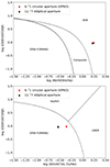 |
Fig. A.1. Emission line ratio (Baldwin–Phillips–Terlevich) diagrams showing the position of the UGC 2885 nucleus. Spectra were extracted in two apertures, with radii of |


All Tables
All Figures
|
Fig. 1. Size–stellar mass relation for local star-forming galaxies in the GALEX-SDSS-WISE Legacy Catalog (Salim et al. 2016) and Siena Galaxy Atlas (Moustakas et al. 2023). The large star indicates the position of UGC 2885, with the stellar mass as reported by Di Teodoro et al. (2023), the SFR as reported by Hunter et al. (2013), D25 from the HyperLEDA database, and the distance given in Table 1. |
| In the text | |
|
Fig. 2. Colour composite of HST/WFC3 images of UGC 2885 (F814W, F606W, and F475W in red, green, and blue, respectively). A bright foreground star (HD279085, V = 10.7) is inconveniently superimposed on the disc. |
| In the text | |
|
Fig. 3. ORBS-processed deep white light flux maps in SN1 (363–386 nm), SN2 (482–513 nm), and SN3 (647–685 nm) filters. Bottom right: Placement of the elliptical apertures used to calculate metallicities and the metallicity gradient. The white circle represents a bright foreground star, which was masked during metallicity calculations. |
| In the text | |
|
Fig. 4. WISE images of UGC 2885 in bands W1 (3.6 μm; grey scale) and W4 (22 μm; contours). The dashed blue circle is the W1 beam size ( |
| In the text | |
|
Fig. 5. Signal and noise maps derived from the IRAM CO(1−0) datacube. Top left: Peak intensity of the brightness temperature (K) of the original cube. Top right: Noise level (σ) over the spectral range of the cube. The dotted black line represents the average level of noise (σ = 0.0081 K), used to create the following panel. As seen in the central channels, we cannot completely separate the cube’s signal from its noise, even after sigma-clipping. Bottom left: Noise model, or the spatial distribution of noise to be subtracted from the original map. Bottom right: Region with signal that surpasses 5σ. The dashed red circle in the upper-right corner shows the 22.49 arcsec beam size of the IRAM observation. |
| In the text | |
|
Fig. 6. CO moment maps of UGC 2885 from the IRAM datacube. Top: Moment-0 (integrated intensity) map. Middle: Moment-1 (intensity-weighted velocity) map. Bottom: Moment-2 (square root of the intensity-weighted dispersion, or line width) map. The dashed box in all panels highlights the central region. The box is |
| In the text | |
|
Fig. 7. Distribution of the brightness temperature in a channel of the datacube. σCO is the channel standard deviation, here taken as the spectral noise. The dotted green lines are spaced 1σ from the mean value. |
| In the text | |
|
Fig. 8. Distribution of H I emission in UGC 2885 from the WSRT data (red contours). Each increment represents 100 Jy beam−1 km s−1. The background filled map is the integrated flux (moment-0) from the IRAM datacube. The blue box is as described in Fig. 6. The dashed red circle is the IRAM beam size, and the solid red ellipse is the WSRT beam size (13 × 19 arcsec). |
| In the text | |
|
Fig. 9. Metallicity calculated using N2O2, R23, and O3N2 diagnostics. The specific radial zones evaluated were 0–10 kpc (ellipse A), 10–20 kpc (ellipse B), and 20–25 kpc (ellipse C). The overall metallicity values calculated with N2O2 and R23 agree well, with the O3N2 metallicity offset to a lower value. None of the three indicators shows a strong metallicity gradient. |
| In the text | |
|
Fig. 10. SFMS of the xCOLD GASS sample with available ALFALFA H I fluxes. The solid line is the SFMS, and the dashed lines show ±0.4 dex scatter as described by Saintonge et al. (2017). Colour represents the depletion time (tdep) of the molecular gas (left panel) and atomic gas (right panel). |
| In the text | |
|
Fig. 11. SFR as a function of stellar mass for a sample of massive disc galaxies (Lisenfeld et al. 2023) colour-coded by their molecular-to-stellar mass ratio (MH2/M⋆). UGC 2885 is displayed for comparison but was not included in the fitting of the SFR–M⋆ plane. The range of stellar masses differs from that of Fig. 10, as super-spiral galaxies have logM⋆ > 10.47 M⊙. |
| In the text | |
|
Fig. 12. Relation between the galaxy stellar mass, SFR, and metallicity based on the data from Mannucci et al. (2010). The orange star represents UGC 2885’s position in the chart based on our calculated values: stellar mass log(M⋆)=11.68 and SFR log(SFR)=0.48. The blue star represents UGC 2885’s position in the chart based on previous values (log(M⋆)=11.3, log(SFR)=0.40; Hunter et al. 2013). Both metallicities found using the FMR are comparable to the results found using the emission line diagnostics to calculate metallicity (Z ≈ 9). |
| In the text | |
|
Fig. 13. Molecular hydrogen mass as a function of stellar mass (molecular gas main sequence) for the xCOLD GASS sample. The sample is colour-coded by SFR. UGC 2885 is far above the relation due to its large gas reservoir. |
| In the text | |
|
Fig. A.1. Emission line ratio (Baldwin–Phillips–Terlevich) diagrams showing the position of the UGC 2885 nucleus. Spectra were extracted in two apertures, with radii of |
| In the text | |
Current usage metrics show cumulative count of Article Views (full-text article views including HTML views, PDF and ePub downloads, according to the available data) and Abstracts Views on Vision4Press platform.
Data correspond to usage on the plateform after 2015. The current usage metrics is available 48-96 hours after online publication and is updated daily on week days.
Initial download of the metrics may take a while.