| Issue |
A&A
Volume 699, July 2025
|
|
|---|---|---|
| Article Number | A85 | |
| Number of page(s) | 9 | |
| Section | Stellar atmospheres | |
| DOI | https://doi.org/10.1051/0004-6361/202451314 | |
| Published online | 01 July 2025 | |
Atmospheric dynamics and shock waves in RR Lyr
II. Helium emission occurrence★
1
Observatoire de Haute-Provence – CNRS/PYTHEAS/Université d’Aix-Marseille,
04870
Saint Michel l’Observatoire,
France
2
Observatoire d’Oukaïmeden, Faculté des Sciences et Techniques, Université Cadi Ayyad,
LPHEA,
Marrakech,
Morocco
3
Observatoire du Val de l’Arc,
13530
Trets,
France
4
Observatoire des Tourterelles,
34140
Mèze,
France
★★ Corresponding authors: denis.gillet@osupytheas.fr; sefyani@uca.ac.ma; bma.ova@gmail.com
Received:
30
June
2024
Accepted:
17
April
2025
Context. This second paper about atmospheric dynamics and shock waves in RR Lyr focuses on the occurrence of the faint helium emission lines of this star.
Aims. We determine the frequency of the appearance of helium emission during the whole pulsation cycle and its connection with atmospheric dynamics.
Methods. We used 1268 high-resolution spectra over a total of 40 nights that were made with the spectrograph ELODIE (Haute Provence observatory, France) during 1994–1997. A detailed analysis of the line profile variations over the whole pulsation cycle was performed to detect the possible presence of helium emission during the survey. The shock wave velocity and emission line intensity were used as indicators of activity in the atmospheric dynamics.
Results. All of these observations show that the helium emission line He I D3 (5875.66 Å) is present in at least half of the observations and in all Blazhko phases. For a shock velocity estimated between 100 and 150 km s−1, the He I D3 line intensity reaches a maximum around Vshock ∼ 123 km s−1, and it then decreases while Vshock still increases. This phenomenon is certainly induced by the ionization of He I. The threshold shock velocity under which He I cannot be observed in emission is probably lower than 100 km s−1. Due to the moderate signal-to-noise ratio of the observations we used in our study, the ionized helium line He II (4686 Å) was probably detected five times. The exhaustive detection of He II in emission requires a high signal-to-noise ratio (>200) and at least one resolving power of 10 000.
Conclusions. Finally, in contrast to what is widely accepted today, the neutral helium emission lines are certainly present at each pulsation cycle, and therefore, from minimum to maximum Blazhko. The ionization of the helium D3 line is expected to only occur above a critical value of the shock velocity that must be about Vshock ∼ 130 km s−1.
Key words: shock waves / stars: atmospheres / stars: oscillations / stars: variables: RR Lyrae
Publisher note: A paragraph "Erratum" indicates the error in Table 2 of Paper I (https://doi.org/10.1051/0004-6361/202347355).
© The Authors 2025
 Open Access article, published by EDP Sciences, under the terms of the Creative Commons Attribution License (https://creativecommons.org/licenses/by/4.0), which permits unrestricted use, distribution, and reproduction in any medium, provided the original work is properly cited.
This article is published in open access under the Subscribe to Open model. Subscribe to A&A to support open access publication.
1 Introduction
It is currently well established that strong shock waves cross the atmosphere of RR Lyrae stars during periodic pulsation movements. Observational facts in favor of these waves include the doubling of metallic absorption lines, the appearance of hydrogen lines in emission, and the Van Hoof phenomenon (van Hoof & Struve 1953).
Whitney (1956) found that the emission of helium is possible through the radiation of the compressed gas during the compression of the atmosphere. When the shock velocity is higher than 80 km s−1, it has enough energy to completely ionize the He I and He II. Whitney used a LTE (local thermal equilibrium) shock model, however, and he overestimated the temperature in the wake of the shock.
Abt (1959) and Wallerstein (1959) presented in two consecutive articles a model of a shock wave that crossed the atmosphere of the star RR Lyr. The shock wave started in sub-photospheric layers and propagated toward the outside, where its velocity quickly became supersonic. Without resorting to the LTE hypothesis, the authors deducted that the zone behind the front of the shock wave had to reach a temperature between 40 000 K and 100 000 K, which is sufficient to ionize hydrogen and helium. No helim emission had been detected at that point.
Because helium emission had not been observed, it was not considered from theoretical or observational points of view. For instance, Fokin & Gillet (1997) calculated atmospheric pulsation models with shocks in order to model the evolution of the Hα line, but they did not consider helium emission.
Preston (2009) fortuitously observed five lines of He I in emission and in absorption with the echelle spectrograph (R = 27 000) of the du Pont 2.5 m telescope at Las Campanas Observatory in ten RR Lyrae stars for the first time. He noted that this emission occurred around pulsation phase 0.9 and lasted about 15 minutes. This is barely half the time of Hα. Then, Preston (2011) observed the emission line of He II (4685.68 Å) in three RR Lyrae stars during the maximum of the Blazhko cycle for the first time. He noted that the line doubling of metallic lines is quite strong (ΔRV between 63 km s−1 and 70 km s−1). This suggests that during the shock passage, this latter is intense enough to cause a sharp increase in the temperature that is capable of ionizing helium.
Gillet et al. (2013) used the spectrograph ESPaDOnS, installed at the CFHT (3.60 m), with a resolving power of 65 000 and a signal-to-noise ratio about 180. They were able to observe both He I and He II in emission in RR Lyr spectra. This was the first time that helium emission was observed in RR Lyr itself since its discovery in July 1899 by Mrs. Fleming (Pickering et al. 1901). Gillet et al. (2013) also observed that Hα emission starts at φ = 0.887, just before the emission of He I D3 line (5875.66 Å) in phase 0.902. The intensity maximum of the D3 line was about 7% above continuum, and that of Hα was 27%. The second emission line of He I (6678.16 Å) that was observed by Gillet et al. (2013) had an intensity maximum of about 2% at 0.911. The He II line (4685.68 Å) is also observed at φ = 0.911, but with a very weak intensity between 0.4% and 0.8%. A post-maximum emission on the D3 line was also detected in this survey after the maximum luminosity and lasted up to phase 1.1.
Gillet et al. (2016) observed the spectral profile of the post-maximum emission of the He I D3 line between the phases 0.984 and 1.098 in detail. This profile is a P Cygni profile. It might therefore be the signature of the expanding atmosphere that is induced by strong shocks during the pulsation cycle. It is characterized by weak emission at the end of the Hα absorption line doubling.
The emission of He I D3 line was observed in different Blazhko phases since 1994 and was confirmed during the observations made at the Oukaïmeden observatory in 2013, but no He II emission was detected (Sefyani et al. 2021). Moreover, the observation of the second emission line of He I (Gillet et al. 2016) was accompanied by a doubling of the Fe II 4923.921 Å and 4549.214 Å metal lines (Sefyani et al. 2017, 2018). The analysis of the these 2015 Oukaïmeden observations showed that no He II emission was detected either, most probably because the average signal-to-noise ratio (S/N) was too low (<10).
Finally, surprisingly and after more than half a century of spectroscopic observations, no specific study of the occurrence of helium emissions in the brightest RR Lyrae star has been carried out, although it was first detected in a few RR Lyrae stars by Preston 2009. Moreover, based on the set of detections, the presence or absence of the helium emission does not seem systematic. This appearance might therefore only occur during pulsation cycles with an exceptional amplitude. The objective of our study is to determine the appearance frequency of the helium line in RR Lyr.
We present observations of profile variations in helium lines in RR Lyr. In Sect. 2 we describe the observed data and their reduction processes. We analyze the observations in Sect. 3, especially the occurrence of the helium line in emission. We considered the D3 He I (5875.66 Å), the He I (6678.16 Å), and the He II (4685.68 Å) line. The consequence of the frequency of the helium emission is discussed in Sect. 4, as well as its effect on the dynamical structure of the atmosphere. Finally, we draw our conclusions in Sect. 5.
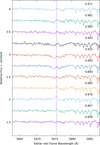 |
Fig. 1 Evolution of the He I λ5875.66 (D3) line profile of RR Lyr corresponding to the night of August 1, 1996 (ψ = 1.10), within the pulsation phase indicated on the right side. The first D3 line emission is visible between 0.859 ≤ φ ≤ 0.894 and is followed by the P Cygni profile (second D3 emission) between 0.903 ≤ φ ≤ 0.961. The exposure time was 300 s, and the absorption lines beyond 5880 Å are telluric lines. The vertical line represents the D3 line laboratory wavelength. The profiles are presented in the stellar rest frame and are arbitrarily shifted in flux for visibility. |
2 Observations and data analysis
The spectral data set we analyzed is the same as we discussed in the first article (Gillet et al. 2023; hereafter Paper I), but it is limited to spectroscopic observations made in 1994–1997 at the Observatoire de Haute Provence (CNRS), France, here-after OHP. The data consist of 1268 spectra that were recorded over 40 nights. The mean signal-to-noise ratio (S /N ∼ 30) and resolving power (42 000).
The data from 1994–1997 are spread over 10 different Blazhko cycles. The occurrence of the Hα and He I D3 emission lines is summarized in Table 1. In the 19 observation nights that were analyzed in 1994–1997, we reliably observed the He I D3 emission ten times, and it was doubtful once. The He II emission was certainly detected twice and probably detected twice as well.
The details of the data acquisition, data reduction, and ephemeris computation were given in Paper I. In addition, the line analysis such as the equivalent width (EW) measurements in this paper were made with the SpcAudace software (Mauclaire 2017), and we trailed the spectra with an internal Python script. The pulsation phase is denoted φ, where φ = 0.0 corresponds to the luminosity maximum and the Blazhko phase ψ, and it has its maximum at ψ = 0.0 when the highest luminosity amplitude is observed during a Blazhko cycle (∼40 d).
Observation log of the RR Lyr spectra around maximum luminosity.
3 Observations of helium in RR Lyr
The emissions of helium lines were detected in the star RR Lyr for the first time by Gillet et al. (2013) just after a Blazhko maximum (ψ ≈ 0.1) with a 4 m class telescope (CFHT) and an exposure time of a few minutes. The S/N was about 200. The emission was observed during the night of July 4, 2011, on the D3 He I (5875.66 Å), the He I (6678.16 Å), and the He II (4685.68 Å) lines. With a resolution power of approximately 65 000, the visibility of the line profiles was easily achieved even though the maximum intensity of He II remained very low (0.4% above the continuum). Because during this pulsation cycle, the estimated shock velocity was moderate (126 km s−1), the presence of the He II emission line should therefore often be potentially observable. However, as it seems rarely detected, this is obviously due to an insufficient S/N of the observations in general.
Because helium emission appears to occur at the same phases as hydrogen emission, that is, just before maximum luminosity of the pulsation cycle, we first spotted nights when the Hα line is in emission. In the 1994-1997 data set, we found a maximum luminosity in 19 out of the 40 nights when the Hα line was in emission. Finally, our analysis of the possible occurrence of helium emissions (He I (5875.66 Å), He I (6678.16 Å), and the He II (4685.68 Å)) focuses on these 19 nights.
3.1 First helium D3 line emission
The D3 line profile was measured in the night of August 1, 1996, just after the Blazhko maximum (ψ = 1.10) between pulsation phases 0.859 and 0.971 (Figs. 1 and 2). In this range of pulsation phases, the D3 line was present in emission or in absorption or both (P Cygni profile). Then, a weak (IMax − Ic = 3%; see Table 1) but clearly visible emission was observed from pulsation phase φ = 0.867 until 0.885, when the Hα and Hβ emission was most intense. This means that the helium D3 emission is also produced by the main shock wave. Just after this, between pulsation phases 0.894 and 0.971, the D3 line profile appeared in absorption before it disappeared.
Out of all the observations we analyzed (1994 to 1997), we detected the D3 emission of helium in approximately 50% of the observations (see Table 2). For all of our spectra, the S/N is between 11 and 55 (see Table 1). Ideally, an S/N of 200 is desirable for confidence. Consequently, our detection rate of the D3 line is probably higher than 50% in the spectra that are likely to show a hypothetical emission of this D3 line.
Nineteen of the 40 observation nights between 1994 and 1997 included a pulsation phase with a maximum at the first D3 helium emission line. This latter occurred around pulsation phase φ = 0.90 ± 0.02 and is well correlated with the hydrogen emission of the first apparition, that is, the main shock. Figure 3 shows these spectral profiles of the D3 emission at their maximum intensity and their corresponding Blazhko phase. We found that the D3 emission is weak, with a maximum residual flux value of 8% (August 5 and 6, 1997; see Table 1), very weak (1%), or absent, that is, not detectable. For example, during the night of June 25, 1996 (ψ = 0.15), the D3 emission was not observed, but the residual flux for Hα was 18%.
The emission with the highest intensity occurred at Blazhko phase 0.56 ± 0.04, that is, just after the minimum of the Blazhko cycle, as shown in the evolution of the EW of the He I λ5875.66 line (D3) in Fig. 4. Because there are only a few measurements and they are dispersed, we measured the minimum EW on the fitting curve to avoid having to rely on an individual measurement. The corresponding value of Vshock ≃ 123 km s−1 to the EW maximum was obtained from Gillet et al. (2023), Fig. 6.
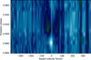 |
Fig. 2 Dynamical spectrum of the time series of the He I λ5875.66 (D3) line profile of RR Lyr corresponding to the night of August 1, 1996 (ψ = 1.10). This figure highlights the second emission of the D3 line with a P Cygni profile (0.920 ≤ φ ≤ 0.965) that follows the first emission (0.860 ≤ φ ≤ 0.900). The absorption component in dark green is located at about −38 km s−1 from the emission component that rose from φ ≃ 0.925 to φ ≃ 0.970. The vertical dark features are telluric lines. The velocities are given in the stellar rest frame, and positive velocities correspond to inward motion (toward the photosphere). The pulsation phases are shown on the left side. |
Summary of the occurrence of emission lines of Hα, He I 5875 Å, and He II 4686 Å.
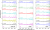 |
Fig. 3 Evolution of the He I (5875.66 Å) line profile of RR Lyrae at different Blazhko phases recorded for 1994–1995, 1996, and 1997. The vertical line indicates the laboratory wavelength of the He I line. The Blazkho ψ and pulsation phases φ are given right and left of each spectrum, respectively. The resolving power is 42 000. |
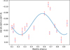 |
Fig. 4 Equivalent width evolution of He I (5875.66 Å) emission line component measured at each pulsation maxima in the 1994–1997 dataset. The integration width is between 5874.5–5877 Å, where EW < 0 corresponds to emission contributions. A fitting with a sine function shows the EW trend with a maximum at ψ ≈ 0.56 ± 0.04. |
3.2 Second helium D3 line emission
After the main D3 emission around φ = 0.92, a second D3 emission was detected for the first time by Gillet et al. (2016) in an observation (October 12, 2013) made at the Oukaïmeden Observatory after the Blazhko maximum (ψ = 0.16 ± 0.08), that is, after the time when the strongest shocks occur during the Blazhko cycle. This second emission presents a P Cygni profile. It was well observed in the average of only five spectra (their Fig. 5).
In the 19 observation nights between 1994 and 1997 at OHP during which this interval was covered, the second helium emission was almost always detected following the appearance of the first emission. The intensity of the P Cygni emission was well above the continuum for 9 nights, low for 2 nights, and moderate for the other 6 (see Table 2). For example, during the night of September 5, 1995 (ψ = 1.60), the second D3 emission was detected in the average of 2 spectra between phases 1.017 and 1.085 (Fig. 5).
Gillet et al. (2013) did not mention the detection of the second helium D3 emission during the night of July 4, 2011, at CFHT. Their 2D time series of this line (their Fig. 3) prevents us from highlighting this second emission, which should be visible approximately between phases 1.02 and 1.06. Thus, no P Cygni emission is detectable during this pulsation cycle, in which the maximum shock velocity was relatively moderate (126 km s−1).
3.3 Helium line HeI λ6678.16
The emission of the helium line He I λ6678.16 (singlet) is also expected to occur around pulsation phase 0.92 when Hα reaches its emission maximum. This helium line must be weaker than the He I λ5875.66 (triplet), as previously noted (Gillet et al. 2013).
Thus, the lack of a detection is probably caused by a too low S/N rather than a weak intensity of the main shock wave. In the observation on October 12, 2013 (Gillet et al. 2016), during which He I λ6678.16 was seen in emission, the shock velocity was estimated at only 117 km s−1. During our observation at CFHT (July 4, 2011), however, which was carried out with a good S/N (∼200), the emission of this helium line was detected near φ = 0.911, but its intensity was very weak (∼2% at its maximum) compared to that of D3 (∼7%), even though the shock velocity was126 km s−1
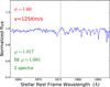 |
Fig. 5 He I λ5875.66 line (D3) P Cygni profile of RR Lyr from the night of September 5, 1995 (ψ = 1.60), obtained by coadding two spectra at pulsation phases of 1.017 and 1.085. The second D3 emission is expected to occur within this pulsation phase range. The position of D3 is marked by a vertical line. |
3.4 Helium line He II λ4685.68
The He II (4685.68 Å) in emission was probably observed during the night of October 12, 2013 (ψ = 0.16, Vshock = 117 km s−1 Gillet et al. 2016). Only 4 of the 19 observation nights in 1994– 1997 around φ = 0.92 probably presented He II in emission (e.g., Fig. 6): September 5, 1995 (ψ = 0.60, Vshock = 126 km s−1), October 17, 1995 (ψ = 0.67, Vshock = 128 km s−1), June 11, 1997 (ψ = 0.26, Vshock = 129 km s−1), and August 30, 1997 (ψ = 0.30, Vshock = 124 km s−1). The He II emission does not appear to depend on Blazhko phases and does not need Vshock to reach the highest values measured in this data set, that is, 149 km s−1. As an example, the trailed spectrum (Fig. 7) shows that He II emission is detected despite the low S/N of the spectra obtained with 300 s single exposures in the 1995 September 5 (1995-09-05) time series.
The analysis of the spectra of June 11, 1997, shows more clearly that the He II emission is visible in two consecutive spectra (φ = 0.894 and 0.900). The maximum in the emission of Hα as the single occurrence of the maximum He I D3 occurs just before (φ = 0.887), while He II occurs later (φ = 0.894). As part of the temporal resolution of these observations, this delay of one hundredth of a pulsation period corresponds to 8 minutes. This undoubtedly indicates that the He I atoms were not yet ionized when the shock penetrated the relevant atmospheric layers.
In addition to our He II 4685.68 Å detections, an observation at the CFHT in 2011 shows that it was possible to highlight helium in emission despite the moderate shock velocity(126 km s−1). The maximum intensity of this emission was still very low, however (0.4%, which is just above the continuum).
The lack of a detection is certainly the consequence of a too low S/N or/and a too low temporal resolution, which prevent a good detection. A definitive detection would therefore require a telescope of the 3 m class or higher in order to achieve a S/N of at least 200 in 5 minutes of integration time with at least one resolving power of 10 000.
4 Analysis of the helium emission
The excitation of the hydrogen and helium lines occurs in the shock wake just after the thermalization zone. Fadeyev & Gillet (2001) showed that for shock velocities as low as 50 km s−1, the thermalized temperature is already about 20 000 K. In the physical conditions in the radiative wake of a stellar shock, which deviate from LTE, the excitation of He I must therefore reach a peak of about 25 000 K and start to be perceptible from 10 000 K, while for He II , this should be 50 000 K and 30 000 K, respectively. Consequently, for the shock velocities between 110 and 150 km/s that we already observed in RR Lyr (Table 1), we expect that helium is notably excited, and this would therefore allow us to observe the corresponding emission lines.
Consequently, the emission lines of helium that can currently be detected enable us to know whether a high-intensity shock wave is present or absent in the atmosphere. These waves appear when the shock reaches a critical speed. The critical speed depends both on the physical state of the atmospheric gas in front of the shock and on the force of the latter, that is, its propagation velocity.
Furthermore, as shown below, the profile variations in certain helium lines during the pulsation phase enable us to high-light the development of the dynamics in the atmosphere. This information is complementary to the information that is provided in part by the observation of hydrogen emission.
The spectra we analyzed that showed Hα emission included 60% in which He I 5875 Å was also in (first) emission for only 20% He II 4686 Å (see Table 2). These detection rates are certainly below reality because the S/N ratio of these spectra is rather moderate. We therefore only considered the D3 He I line at 5875.66 Å for a relevant detection and for the analysis below.
4.1 Analysis of the D3 helium emission
4.1.1 Analysis of the first D3 helium emission
As already mentioned in the introduction, the presence of helium in emission was discovered by Preston in 2009 with a 2.5 m telescope. This is surprising because the RR Lyrae stars, and in particular, the brightest of them, RR Lyr itself, have been widely observed in spectroscopy since the 1950s. Until the early 1980s, receptors that were only photographic plates were hardly able to achieve an S/N greater than 100. In addition, the use of telescopes in the 4 m class or higher was rare. These instruments are large enough to reach a time resolution of a few minutes, which is required in order to be able to capture the elusive and weak emission of helium.
Out of all the observations between 1994 and 1997 we analyzed, 19 observation nights covered the 0.92 pulsation phase. Around this phase, the emission of hydrogen must be observed because the passing of the main shock in the atmosphere is very intense. Hα emission was observed each time. Simultaneously with this main Hα emission, a weak emission of the D3 helium line was clearly observed for 10 (60%) out of the 19 nights (Table 2). This detection rate might approach 100% if an S/N of several hundred percent were reached.
For the nights for which we consider that the detection of the emission of D3 is secure, no obvious correlation between the shock intensity (therefore its velocity) and the intensity of the D3 emission line is visible (Table 1). For example, forshock velocities of 120, 124, and 111 km s−1, we obtain intensities above the continuum of 5%, 5%, and 4% respectively, while for higher shock velocities (149, 146, and 143 km s−1), we measure similar or lower values (4%, 0%, and 3% respectively). The highest-intensity values 11% and 8% were measured at intermediate shock velocities (125, 134, and 139 km s−1). When the shock velocity increases, the helium is clearly increasingly ionized, which is expected to generate a decrease in the intensity of D3. This is observed for velocities higher than 140 km s−1. We note, however, that the dynamics of the atmosphere from one pulsation cycle to the next can be quite different because of the movement history of the atmospheric layers induced by previous cycles. The amplitude of the ballistic movement of the layers and their dynamic relaxation are both certainly far from being reproducible and must generate non-negligible differences between the pulsation cycles. These irregularities in the atmospheric dynamics might help us to understand why, for example, an intensity as high as 5% with respect to the continuum is observed for D3 when a shock velocity as low as 120 km s−1 is observed (Table 1).
Fig. 4 shows that the equivalent width of He I reaches a maximum around Blazhko phase 0.56, that is, just after the Blazhko minimum. Irregularities in pulsation cycles must contribute significantly to the dispersion of the EW points. Because the shock velocity reaches its minimum at the Blazhko minimum and then again starts to increase (see Fig. 6 of Paper I), helium will clearly be increasingly ionized within the radiative shock wake as the Blazhko maximum is approached. Consequently, as we know that neutral helium cannot be excited in the atmosphere when it is not affected by the shock wave, it is logical that the EW of He I decreases between the Blazhko minimum and maximum. Furthermore, in Fig. 9 of Paper I, the maximum Hα intensity occurs in Blazhko phases 0.1 and 0.9 for a shock velocity of about 138 km s−1, while in our Fig. 3, the maximum EW of the helium D3 line occurs at Blazhko phase 0.56 for a velocity of about 123 km s−1. Depending on the physical conditions occurring both in the atmosphere and in the radiative shock wake, the ionization of D3 therefore occurs when the shock velocity is typically between 123 and 138 km s−1, that is, for a mean value of about 130 km s−1.
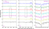 |
Fig. 6 Evolution of the hydrogen and helium emission line profile of RR Lyr during the night of June 11, 1997. Panel a: two consecutive weak He II 4685.68 Å emissions at φ = 0.894 and φ = 0.900 are assumed to be present. Their intensity above the continuum is 6% and 7%, wich is just slightly higher than the D3 He I emission line. Panel b: three consecutive He I 5875.66 Å emissions with an intensity of ∼5% above the continuum are observed, starting at φ = 0.887. Panel c: variation in the Hα profile that reaches 33% above the continuum. The Blazhko phase and the shock velocity are indicated in the top left corner of panel a) and the pulsation phase is shown in the left corner above each spectrum in panel b). The laboratory wavelength of the spectral line of interest is marked by a vertical line in each panel. |
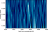 |
Fig. 7 Trailed spectrum of He II line (4685.68 Å) build with eight spectra from the time series of September 5, 1995. The He II emission is visible from φ ∼ 0.927 to φ ∼ 0.937 (two consecutive spectra) as a short bright vertical spindle despite the weak signal. The He II emission follows the He I λ5875.66 first emission, which occurred between φ ∼ 0.906 − 0.925, as expected. The vertical white line indicates He II laboratory wavelength. |
4.1.2 Analysis of the second D3 helium emission
The second emission of the D3 helium line (P Cygni profile) occurs approximately one hour after the first emission, that is, between pulsation phases 1.03 and 1.05. The intensity of the second emission of D3 and that of the P Cygni profile are clearly not correlated. For example, during the nights of August 5 and 6, 1997, which correspond to the same Blazhko cycle (2.66 and 2.69; see Table 1), the intensity of D3 was very high and the same (I = 8%), while the intensity of the P Cygni profile was weak and high, respectively. During these two cycles, the shock velocity was similar (139 and 134 km s−1), and the signal-to-noise ratio of the spectra near λ6557 was 39 and 29, respectively.
4.2 Comparison between D3 helium and Hα P Cygni profiles
The P Cygni profile of D3 occurs just after the pulsation phase 1.03 during a short period of time (up to 15 minutes or Δφ ≃ 0.02). It comes just after the end of the Hα doubling (φ ≃ 1.03). In contrast, the P Cygni profile of Hα occurs significantly later, and it is visible approximately between pulsation phases 0.2 and 0.4. The emission of the Hα P Cygni profile reaches its maximum in phase 0.3.
The helium D3 line in emission cannot be produced in atmospheric layers that have not yet been crossed by the shock because their temperature is insufficient. It can only be produced in the radiative wake of a shock. Thus, unlike Hα, there is no photospheric absorption component of D3 because the excitation potential of helium is clearly higher (+11 eV) than that of Hα. Consequently, the duration of the double absorption of D3 is four times shorter than that of H α (Δφ≃ 0.025 compared to 0.10). Moreover, because the shock velocity decreases rapidly from the photosphere, it is logical that the P Cygni profile of D3 is observed in the lowest part of the atmosphere.
The emission component of the P Cygni profile of Hα is located where the red component of Hα occurs during its doubling. This latter absorption component is much larger and more intense than the narrow emission of the P Cygni. Consequently, it is necessary to wait until this absorption component of Hα disappears to begin distinguishing the weak emission, that is, around pulsation phase 0.2 (see Figs. 2 and 3 of Gillet et al. 2019).
In the stellar rest frame, the intensity maximum of the D3 P Cygni emission is centered on the laboratory wavelength (zero velocity). This profile was first reported by Preston (2009) in the RRab star RV Oct. Then, Gillet et al. (2016) observed the same P Cygni profile in RR Lyr, that is, with the emission maximum centered at the zero velocity. This is not at all the case for the P Cygni profile of Hα because the emission is largely redshifted (Gillet et al. 2017). As shown by Bertout (1984), when a high-velocity field is present in an emitting atmospheric region (here: the radiative shock wake), the Doppler shift decouples the different emitting layers when the gas velocity exceeds the local line profile width. In this case, the maximum of the P Cygni emission is therefore centered at the zero velocity, and the Sobolev approximation can be used to compute the line source function. The stronger the decrease in the maximum velocity of the flow, the stronger the redshift of the emission. This shift is appreciable immediately below ten units of the atomic thermal velocity. However, other parameters such as the geometric extension of the emitting layer or the anisotropy effect of the radiation field produced by the shock wave can also play a role in the formation of the line profile (Wagenblast et al. 1983).
As established by Bertout (1984), when the P Cygni emission is redshifted and all the more so as it is, the absorption minimum becomes a good indicator of the maximum velocity of the expansion. For example, we measured a velocity of the D3 P Cygni absorption minimum of about 20 km s−1 during the night of August 31, 1997, and at about 38 km s−1 during the night August 1, 1996, which approximately corresponds to a Mach number of 2 and 4, respectively. This means that the expansion of the shock shell is barely supersonic at the beginning of the pulsation interval 1.2 ≲ φ ≲ 1.4 during which the P Cygni emission is in principle observable. Unfortunately, the observations of the night of August 31, 1997, end at φ = 1.197, and therefore, it is not possible to know the change with altitude in this expansion velocity. The observations reported by Gillet et al. (2017) during the nights of September 4, 2013, and September 14, 2014, however, indicated that the velocity of the shock shell slowly decreased from φ ≃ 1.175 to φ ≃ 1.382. The whole atmosphere undergoes this decreasing movement because it is mainly driven by the shock. For these two phases (of different nights), the shock velocity was 40 and 20 km s−1, respectively. This last value is consistent with the value estimated for the night of August 31, 1997. During this phase interval, the shock wave therefore decelerated continuously and passed from a Mach number of 4 to Mach 2. It therefore experienced a very low supersonic velocity that increasingly decreased until the shock disappeared in the upper atmosphere. This latter also occured with the maximum extension of the atmosphere, which finally fell back on the photosphere through gravity.
The P Cygni profile of D3, whose emission is approximately centered on the laboratory wavelength in the stellar rest frame, enables us to measure an expansion velocity of 62 km s−1 on October 12, 2013 (Gillet et al. 2016), for example. Generally speaking, the shock velocity is about 60 km s−1near pulsation phase 1.04. Thus, the shock velocity, which is between 100 and 150 km s−1 when the shock emerges from the photosphere, decreases rapidly up to 60 km s−1 around phase 1.04 (Gillet et al. (2019) Fig. 8a), to then more slowly reach 20 km s−1 when the atmosphere reached maximum extension toward phase 1.40. At this moment, the shock was no longer radiative and dissipated into the outer layers of the atmosphere.
As discussed by Gillet et al. (2019), the shock deceleration occurs in two distinct stages, as shown in their Figs. 8a and 8b. The first stage is during a very short interval (about 5% of the pulsation cycle from φ = 0.89 to 0.95), just after the shock appears. It is strongly hypersonic, with a Mach number between 10 and 16. This implies that the shock radiates a large fraction of its energy. Fadeyev & Gillet (2001) showed that in a pure hydrogen gas and for physical conditions in the atmospheres of pulsating stars, at least 70% of the shock energy is lost in radiative form as soon as the shock velocity is greater than 50 km s−1. This result is reinforced when we also consider the cooling due to Fe lines, which must be very efficient in the atmosphere of low-gravity stars and therefore has a low radius-to-mass ratio(R/M), as do RR Lyrae (Fokin et al. 2004). In these stars, the hot wake is expected to be considerably reduced, so that the expected line emission, including Hα, is probably less prominent than in stars with a high R/M ratio, as observed. The emission intensity in H lines is moderate in RR Lyrae stars despite the very high shock amplitude of up to 150 km s−1, unlike for stars with a high R/M ratio, such as W Virginis, RV Tauri, and Mira stars.
Gillet et al. (2019) showed that at the maximum, the radiative losses of the shock vary up to the third power of the shock front velocity. As their observations indicated (Figs. 8a and b), the decrease in the shock velocity slows down sharply up to 100 km s−1 from around φ = 0.93. A second, more hydrodynamic regime is then set up. The radiative losses become secondary, and the shock energy mainly decreases by geometric dilution (1/r2) as the shock radius r increases. Finally, the remainder of the shock energy is dissipated by dilution in the high atmosphere when the radiative nature of the shock is no longer dominant.
 |
Fig. 8 Line profile evolution of Hα, D3 He I and Na D vs. the pulsation phase from minimum Rmin to maximum Rmax of the photospheric radius. The apparition of the strongest Hα emission near 0.89 at Rmin corresponds to the emergence of the main shock from the subphotospheric layers. The letter e means that an emission is present within the Hα line profile (yellow). The blueshifted and redshifted absorption components are shown in blue and red. A P Cygni profile is shown in green. The shock velocity corresponds to an average velocity deduced from Fig. 8 of Gillet et al. (2019). For D3, the dotted area indicates that no emission or absorption line could be detected. The scale and phases are approximate. |
4.3 Effects of atmospheric dynamics on the line profiles
To summarize, the main shock arises from the photosphere near pulsation phase 0.89/0.90 when the two main emissions of Hα and D3 appear almost simultaneously (Fig. 8). D3 lags by about Δφ = 0.01, because its much lower intensity delays the time of its detection. Then, after the line doubling of D3 for about 20 minutes, a P Cygni profile appears about one hour later, but for a short time (up to 15 minutes). With an average velocity of 135 km s−1, the shock wave will have traveled a distance approximately equal to a quarter of the photospheric radius (Rph ≃ 5 or 6 R⊙) before this P Cygni profile can be observed. This time (distance) is therefore necessary for helium, which is only produced in the narrow radiative wake of the shock, to be observed detached from the photosphere. Then, for about 2 hours and 11 minutes (16% of the pulsation period), Hα only presents its photospheric absorption profile and D3 is absent in absorption and emission. The shock wave was thus able to travel in all discretions over a quarter of the photospheric radius without affecting these two line profiles. Finally, from phase 1.2, a P Cygni profile of Hα appears, about 2 hours after the disappearance of that of D3. The enormous width of the photospheric absorption component of Hα and its splitting phase both delayed the visibility of the photospheric detachment of the shock on this line. This detachment phase is observed over more than 2 hours and 43 minutes or 20% of the pulsation period, approximately up to phase 1.4, that is, until the maximum extension of the photosphere and the most dense atmospheric layers.
5 Conclusion
Our principal aim was to determine the occurrence of helium emission lines in the atmosphere of RR Lyr during its pulsation cycle and its variation with the Blazhko cycle based on spectral observations. Although Wallerstein (1959) theoretically predicted the occurrence of He I emission lines in RR Lyrae stars, this was only accidentally observed by Preston (2009) for the first time in April 2006 in a few RR Lyrae stars. In July 2011, Gillet et al. (2013) detected this emission in RR Lyr itself. The presence of helium emission lines was considered exceptional before. It was assumed that helium in emission could only occur when a very strong intensity shock wave propagates in the atmosphere. Examination of spectra made between 1994 and 1997 showed, however, that the D3 emission line of neutral helium is detected in at least half of the 19 observation nights. The previous lack of a detection of the helium D3 emission line was certainly due to the poor sensitivity of the photographic plates that were used to record these spectra. In addition, the low intensity of the helium emission and its short duration (around 15 minutes) do not favor its detection.
In contrast to what is widely accepted today, the neutral helium emission lines are certainly present in each pulsation cycle, and therefore, from minimum to maximum Blazhko. Our measurements of Vshock show that this latter is always larger than 100 km s−1, which leads to a temperature above 25 000 K within the radiative shock wake region, which allows the excitation of the He I line (see Fadeyev & Gillet 2001 for the physical conditions in the radiative wake of the shock). However, the emission of D3 was not systematically detected in all spectra we considered, although the wake temperature was higher than 25 000 K. This is probably because the S/N of some of the spectra we used was too low. Moreover, because the shock velocity reached minimum at the Blazhko minimum and then again started to increase, helium is clearly increasingly ionized within the radiative shock wake as the Blazhko maximum is approached. Consequently, it seems very likely that He I D3 emission is present in all Blazhko phases, but with various intensities. Only four dates probably presented the He II emission line spread throughout the whole Blazhko cycle, however, where Vshock reached values from 117 to 129 km s−1. This means that the intensity of the shock wave was always strong enough to excite helium, regardless of the Blazhko phase, because the temperature then always reached ∼ 25 000 K. At minimum Blazhko, the shock velocity was about 100 ±10 km s−1, corresponding to a Mach number of approximately 10, and the threshold below which the helium could not be excited would therefore be lower than these values. Furthermore, the irregularities observed in the intensity of the D3 emission and the apparition of He II may be due to amplitude variations in the atmospheric dynamics in the shock intensity from one pulsation cycle to the next. Future observations will certainly help us to study this matter further and allow us to conclude about it definitely.
On all of these observations, the shock wave velocity seems to reach a maximum around the Blazhko maximum and then to decrease toward its minimum (Gillet et al. 2023). This variation in the shock velocity as a function of the Blazhko phase must be confirmed by more numerous and accurate observations, however. We were unable to find any current explanation apart from that of Gillet (2013) to bridge the relation between spectroscopic observations and the Blazhko effect. Unlike the D3 line of He I, since the He II emission only seems to be observable when the shock velocity reaches a critical value (Vshock ∼ 130 km s−1, but this remains to be determined precisely), its detection or absence would allow us to verify the gradual increase in the shock velocity when maximum Blazhko is approached. This observational test requires a telescope of the 4 m class or higher in order to achieve an S/N of at least 200 in 5 minutes of integration time with a resolving power of 10 000 at least.
Finally, we were able to confirm that the interpretation of the P Cygni profile of Hα that occurs between 1.2 ≲ φ ≲ 1.4 is indeed the consequence of the expansion of the (radiative) shock wake when its detachment from the photosphere becomes observable. This profile might therefore be the continuity of the previously P Cygni profile that was observed (1.03 ≲ φ ≲ 1.05) in the D3 line of He I.
Erratum
We found an error in Table 2 of Paper I (Gillet et al. 2023) concerning the HJD0 of the pulsation ephemeris for 2015. Instead of 57354.322, it should read 57333.396. This date comes from the photometric monitoring carried out at the Oukaïmeden observatory in connection with spectroscopic observations.
Data availability
The original spectra presented in this article can be downloaded from the ELODIE database: http://atlas.obs-hp.fr/elodie/
Acknowledgements
We thank the French OHP-CNRS/PYTHEAS for its support. The present study has used the SIMBAD database operated at the Centre de Données Astronomiques (Strasbourg, France) and the GEOS RR Lyr database hosted by IRAP (OMP-UPS, Toulouse, France), created by J.F. Le Borgne. We would also like to thank Guillaume Bertrand for his efficient help with our Python developments. This work was carried out in part within the framework of the Groupe de Recherche sur RR Lyrae (GRRR) which is an association of professionals and amateur astronomers leading high-resolution spectroscopic and photometric monitoring of complex phenomena such as the RR Lyrae Blazhko effect. We especially thank the reviewer for his relevant remarks and suggestions.
References
- Abt, H. A. 1959, ApJ, 130, 824 [Google Scholar]
- Bertout, C. 1984, ApJ, 285, 269 [CrossRef] [Google Scholar]
- Fadeyev, Y. A., & Gillet, D. 2001, A&A, 368, 901 [NASA ADS] [CrossRef] [EDP Sciences] [Google Scholar]
- Fokin, A. B., & Gillet, D. 1997, A&A, 325, 1013 [NASA ADS] [Google Scholar]
- Fokin, A. B., Massacrier, G., & Gillet, D. 2004, A&A, 420, 1047 [NASA ADS] [CrossRef] [EDP Sciences] [Google Scholar]
- Gillet, D. 2013, A&A, 554, A46 [NASA ADS] [CrossRef] [EDP Sciences] [Google Scholar]
- Gillet, D., Fabas, N., & Lèbre, A. 2013, A&A, 553, A59 [NASA ADS] [CrossRef] [EDP Sciences] [Google Scholar]
- Gillet, D., Sefyani, F. L., Benhida, A., et al. 2016, A&A, 587, A134 [EDP Sciences] [Google Scholar]
- Gillet, D., Mauclaire, B., Garrel, T., et al. 2017, A&A, 607, A51 [NASA ADS] [CrossRef] [EDP Sciences] [Google Scholar]
- Gillet, D., Mauclaire, B., Lemoult, T., et al. 2019, A&A, 623, A109 [NASA ADS] [CrossRef] [EDP Sciences] [Google Scholar]
- Gillet, D., Sefyani, F. L., Benhida, A., et al. 2023, A&A, 680, A97 [NASA ADS] [CrossRef] [EDP Sciences] [Google Scholar]
- Mauclaire, B. 2017, SpcAudace: Spectroscopic processing and analysis package of Audela software, Astrophysics Source Code Library [record ascl:1711.001] [Google Scholar]
- Pickering, E. C., Colson, H. R., Fleming, W. P., & Wells, L. D. 1901, ApJ, 13, 226 [Google Scholar]
- Preston, G. W. 2009, A&A, 507, 1621 [NASA ADS] [CrossRef] [EDP Sciences] [Google Scholar]
- Preston, G. W. 2011, AJ, 141, 6 [Google Scholar]
- Sefyani, F. L., Benhida, A., Benkhaldoun, Z., et al. 2017, in Journal of Physics Conference Series, 869, 012088 [Google Scholar]
- Sefyani, F. L., Benhida, A., Benkhaldoun, Z., et al. 2018, in The RR Lyrae 2017 Conference. Revival of the Classical Pulsators: from Galactic Structure to Stellar Interior Diagnostics, 6, eds. R. Smolec, K. Kinemuchi, & R. I. Anderson, 316 [Google Scholar]
- Sefyani, F. L., Benhida, A., Benkhaldoun, Z., et al. 2021, in RR Lyrae/Cepheid 2019: Frontiers of Classical Pulsators, eds. K. Kinemuchi, C. Lovekin, H. Neilson, & K. Vivas, Astronomical Society of the Pacific Conference Series, 529, 343 [Google Scholar]
- van Hoof, A., & Struve, O. 1953, PASP, 65, 158 [NASA ADS] [CrossRef] [Google Scholar]
- Wagenblast, R., Bertout, C., & Bastian, U. 1983, A&A, 120, 6 [NASA ADS] [Google Scholar]
- Wallerstein, G. 1959, ApJ, 130, 560 [Google Scholar]
- Whitney, C. 1956, Ann. Astrophys., 19, 34 [NASA ADS] [Google Scholar]
All Tables
Summary of the occurrence of emission lines of Hα, He I 5875 Å, and He II 4686 Å.
All Figures
|
Fig. 1 Evolution of the He I λ5875.66 (D3) line profile of RR Lyr corresponding to the night of August 1, 1996 (ψ = 1.10), within the pulsation phase indicated on the right side. The first D3 line emission is visible between 0.859 ≤ φ ≤ 0.894 and is followed by the P Cygni profile (second D3 emission) between 0.903 ≤ φ ≤ 0.961. The exposure time was 300 s, and the absorption lines beyond 5880 Å are telluric lines. The vertical line represents the D3 line laboratory wavelength. The profiles are presented in the stellar rest frame and are arbitrarily shifted in flux for visibility. |
| In the text | |
|
Fig. 2 Dynamical spectrum of the time series of the He I λ5875.66 (D3) line profile of RR Lyr corresponding to the night of August 1, 1996 (ψ = 1.10). This figure highlights the second emission of the D3 line with a P Cygni profile (0.920 ≤ φ ≤ 0.965) that follows the first emission (0.860 ≤ φ ≤ 0.900). The absorption component in dark green is located at about −38 km s−1 from the emission component that rose from φ ≃ 0.925 to φ ≃ 0.970. The vertical dark features are telluric lines. The velocities are given in the stellar rest frame, and positive velocities correspond to inward motion (toward the photosphere). The pulsation phases are shown on the left side. |
| In the text | |
|
Fig. 3 Evolution of the He I (5875.66 Å) line profile of RR Lyrae at different Blazhko phases recorded for 1994–1995, 1996, and 1997. The vertical line indicates the laboratory wavelength of the He I line. The Blazkho ψ and pulsation phases φ are given right and left of each spectrum, respectively. The resolving power is 42 000. |
| In the text | |
|
Fig. 4 Equivalent width evolution of He I (5875.66 Å) emission line component measured at each pulsation maxima in the 1994–1997 dataset. The integration width is between 5874.5–5877 Å, where EW < 0 corresponds to emission contributions. A fitting with a sine function shows the EW trend with a maximum at ψ ≈ 0.56 ± 0.04. |
| In the text | |
|
Fig. 5 He I λ5875.66 line (D3) P Cygni profile of RR Lyr from the night of September 5, 1995 (ψ = 1.60), obtained by coadding two spectra at pulsation phases of 1.017 and 1.085. The second D3 emission is expected to occur within this pulsation phase range. The position of D3 is marked by a vertical line. |
| In the text | |
|
Fig. 6 Evolution of the hydrogen and helium emission line profile of RR Lyr during the night of June 11, 1997. Panel a: two consecutive weak He II 4685.68 Å emissions at φ = 0.894 and φ = 0.900 are assumed to be present. Their intensity above the continuum is 6% and 7%, wich is just slightly higher than the D3 He I emission line. Panel b: three consecutive He I 5875.66 Å emissions with an intensity of ∼5% above the continuum are observed, starting at φ = 0.887. Panel c: variation in the Hα profile that reaches 33% above the continuum. The Blazhko phase and the shock velocity are indicated in the top left corner of panel a) and the pulsation phase is shown in the left corner above each spectrum in panel b). The laboratory wavelength of the spectral line of interest is marked by a vertical line in each panel. |
| In the text | |
|
Fig. 7 Trailed spectrum of He II line (4685.68 Å) build with eight spectra from the time series of September 5, 1995. The He II emission is visible from φ ∼ 0.927 to φ ∼ 0.937 (two consecutive spectra) as a short bright vertical spindle despite the weak signal. The He II emission follows the He I λ5875.66 first emission, which occurred between φ ∼ 0.906 − 0.925, as expected. The vertical white line indicates He II laboratory wavelength. |
| In the text | |
|
Fig. 8 Line profile evolution of Hα, D3 He I and Na D vs. the pulsation phase from minimum Rmin to maximum Rmax of the photospheric radius. The apparition of the strongest Hα emission near 0.89 at Rmin corresponds to the emergence of the main shock from the subphotospheric layers. The letter e means that an emission is present within the Hα line profile (yellow). The blueshifted and redshifted absorption components are shown in blue and red. A P Cygni profile is shown in green. The shock velocity corresponds to an average velocity deduced from Fig. 8 of Gillet et al. (2019). For D3, the dotted area indicates that no emission or absorption line could be detected. The scale and phases are approximate. |
| In the text | |
Current usage metrics show cumulative count of Article Views (full-text article views including HTML views, PDF and ePub downloads, according to the available data) and Abstracts Views on Vision4Press platform.
Data correspond to usage on the plateform after 2015. The current usage metrics is available 48-96 hours after online publication and is updated daily on week days.
Initial download of the metrics may take a while.