| Issue |
A&A
Volume 698, May 2025
|
|
|---|---|---|
| Article Number | A182 | |
| Number of page(s) | 9 | |
| Section | The Sun and the Heliosphere | |
| DOI | https://doi.org/10.1051/0004-6361/202555148 | |
| Published online | 11 June 2025 | |
Sunspot cycles for the first millennium BC reconstructed from radiocarbon
1
Space Physics and Astronomy Research Unit and Sodankylä Geophysical Observatory, University of Oulu, Oulu, Finland
2
Max Planck Institute for Solar System Research, Justus-Von-Liebig-Weg 3, D-37077
Göttingen, Germany
3
Ioffe Physical-Technical Institute, St. Petersburg, Russia
4
Laboratory of Ion Beam Physics, ETH-Zürich, Zürich, Switzerland
⋆ Corresponding authors: ilya.usoskin@oulu.fi; chatzistergos@mps.mpg.de
Received:
14
April
2025
Accepted:
9
May
2025
Context. The relative sunspot number (SN) is the primary index of solar activity since 1610. For earlier periods, the SN can be reconstructed from the concentrations of cosmogenic isotopes, in particular, 14C and 10Be in natural archives. Because the measurement techniques are limited, however, these reconstructions typically provide the SN with a resolution of decades only.
Aims. We reconstruct the first annually resolved SNs for the first millennium BC. They provide a detailed view of the solar cycles over a period for which this was not possible before.
Methods. We reconstructed the SN from high-precision annual measurements of relative decay-corrected 14C concentrations, Δ14C, that cover 1000 to 2 BC. The process is based on the physics-based approach we developed earlier and has the following four steps: (1) The carbon-cycle model is inverted to reconstruct the production rate of 14C, Q. (2) The effect of the varying geomagnetic field on Q is accounted for. (3) The open solar magnetic flux is computed. (4) The flux is converted into SN. A Monte Carlo approach is used to account for the uncertainty of the reconstruction.
Results. We reconstructed the annually resolved SN covering the first millennium BC. Over this period, we identified 93 complete solar cycles with a mean length of 10.5 years. Twenty-three of these cycles are well defined, 21 are reasonably well defined, and the remainder are poorly defined. Our reconstructed SN and previous decadal reconstructions agree very well, but the SN around 1000–920 BC is higher. We found no significant long-term periodicities beyond the 11-year solar cycle.
Conclusions. This reconstruction offers unique insights into the cyclic solar activity for this period of time. This is valuable information for solar dynamo studies and irradiance modelling.
Key words: Sun: activity / Sun: magnetic fields / sunspots
© The Authors 2025
 Open Access article, published by EDP Sciences, under the terms of the Creative Commons Attribution License (https://creativecommons.org/licenses/by/4.0), which permits unrestricted use, distribution, and reproduction in any medium, provided the original work is properly cited.
This article is published in open access under the Subscribe to Open model. Subscribe to A&A to support open access publication.
1. Introduction
Our Sun is an active star whose magnetic activity is produced by the action of the solar dynamo in the convection zone (e.g., Parker 1955; Charbonneau 2020). The activity manifests itself through various phenomena that can also affect the Earth’s environment. The most commonly used index of solar activity is the relative sunspot number (SN), which is based on telescopic observations of sunspots and their groups since 1610 (e.g., Vaquero et al. 2016; Clette et al. 2023). Variations in solar activity are dominated by the quasi-periodic Schwabe cycle. Its length varies between 8 and 14 years (Hathaway 2015). This cyclic activity is modulated by secular variability that ranges between grand minima, such as the Maunder minimum (1645–1715, e.g., Eddy 1976; Vaquero et al. 2015), and grand maxima, such as the Modern grand maximum in the second half of the 20th century (Solanki et al. 2004). Although solar activity has only been directly observed for the past 400 years, the Sun is also expected to have been active at earlier times.
The past solar activity can be quantitatively studied using data of cosmogenic isotopes measured in natural terrestrial archives (e.g., Solanki et al. 2004; Steinhilber et al. 2012). The method is based on the fact that these isotopes, most notably 14C (radiocarbon) and 10Be, are produced in the Earth’s atmosphere through interactions with galactic cosmic rays (GCRs). The flux of these cosmic rays that reaches the Earth is modulated by two primary factors: solar magnetic activity, known as heliospheric modulation, and the Earth’s geomagnetic field, which provides geomagnetic shielding (Beer et al. 2012; Usoskin 2023). Knowing the state of the geomagnetic field in earlier periods through independent paleo- or archaeo-magnetic models, we can estimate the past solar magnetic activity. After this method was developed (Usoskin et al. 2003), many solar activity reconstructions were performed for the Holocene (the current warm-climate geological epoch that began about 11.7 millennia ago) based on cosmogenic isotopes 14C, that is measured in tree trunks, and 10Be, that is measured in polar ice cores (see a review by Usoskin 2023). The reconstructed solar activity is often represented by the so-called cosmic-ray modulation potential ϕ (e.g., Nilsson et al. 2024), but it can also be provided as sunspot numbers (e.g., Wu et al. 2018b), which can readily be used to study the past solar magnetic activity and to model variations in the solar irradiance.
While earlier reconstructions revealed significant long-term variability in the solar activity, they lacked the resolution with which individual Schwabe solar cycles could have been identified. As a result, these cycles were observed solely through direct measurements over the past 400 years, which encompassed 36 to 37 cycles. A critical breakthrough was made recently when high-precision annual measurements of the relative decay-corrected 14C concentrations, Δ14C, were performed for the last millennium (Brehm et al. 2021). The high-quality data enabled the first reconstruction of individual sunspot cycles since 970 AD. This nearly tripled the solar cycle statistic (Usoskin et al. 2021). The breakthrough in accurate annual measurements of radiocarbon opened a new avenue for high-resolution solar variability studies and archaeological dating (Heaton et al. 2024).
A new set of accurate Δ14C measurements covering the period 1000–2 BC was recently published by Brehm et al. (2025), along with a reconstruction of the 14C production rate and the cosmic-ray modulation potential. We present a new full reconstruction of the sunspot activity for the first millennium BC based on these new data and on the method developed by Usoskin et al. (2021).
2. Data
We used a composite series of annual Δ14C data (the relative normalized concentration ratio of 14C to 12C) measured in tree rings as the primary data source for the period of 1000 BC through 2 BC (Brehm et al. 2025; Fahrni et al. 2020). The trees were mostly German oak. The dataset is fully described by Brehm et al. (2025) and is shown in Figure 1a. There are several small gaps (one to two years; 769, 618, 617, 614, and 462 BC) that were interpolated between the neighbouring data points before we processed the data further. This period includes an extreme solar particle event (ESPE) at about 664 BC (Park et al. 2017; O’Hare et al. 2019). The corresponding Δ14C spike is indicated by the red arrow in Figure 1a. Since this spike was caused by solar energetic particles (Cliver et al. 2022), it can distort the reconstruction of the solar cycle and should be removed from the dataset before further analysis. The removal is described in Sect. 3.2.
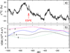 |
Fig. 1. Data for the first millennium BC used here. Panel a: Raw Δ14C data along with the 1σ uncertainties (indicated by the black line and grey shaded band, respectively; Brehm et al. 2025). The red arrow indicates the signature of the ESPE at about 664 BC. Panel b: Paleo- and archaeo-magnetic reconstructions of the virtual dipole moment (VDM), according to 1 Usoskin et al. (2016), 2 Knudsen et al. (2008), 3 Pavón-Carrasco et al. (2014), 4 Schanner et al. (2022), and 5 Nilsson et al. (2022). |
Another independent dataset we used refers to the geomagnetic field as quantified by the virtual dipole moment (VDM) for the same period. The VDM was reconstructed using paleo- or archeo-magnetic models based on natural or archaeological samples with residual magnetization. This process is difficult (Genevey et al. 2008; Korte et al. 2019) and leads to a wide distribution of the modelled VDM values, as shown in Figure 1b. We considered five recent paleomagnetic models covering the entire Holocene that were provided by different groups and methods. The models suggest a different evolution of the VDM that ranges between 8.5 and 11.5 (1022 A m2) for the first millennium BC. The upper and lower bounds of the VDM were set by the models by Knudsen et al. (2008) and Nilsson et al. (2022), respectively. The differences between the independent VDM series by Knudsen et al. (2008) and Usoskin et al. (2016) are small. The challenge in accurately determining VDM forms a major source of uncertainty in reconstructions of the solar activity (Snowball & Muscheler 2007). It is important, however, that the different VDM models are quite smooth, and the difference between them is a systematic or slowly changing offset (on a multi-centennial timescale). Thus, we do not expect this to affect the timing of the reconstructed solar cycles, but it may lead to significant uncertainties in their amplitudes on a long timescale (see Sect. 3.3).
3. Reconstructing the solar cycle
Based on the datasets described above, that is, Δ14C and VDM, we reconstructed the solar activity as quantified in the annual SN for the period from 997 through 7 BC. The first and last few years were excluded as potentially affected by the edge effect in the model when the time resolution of the data switched between a decadal and an annual resolution. The reconstruction was performed using the approach developed by Usoskin et al. (2021). The definition of the SN we considered follows that of the International Sunspot Number, version 2 (ISN-v2 – Clette & Lefèvre 2016).
3.1. Reconstruction chain
The method of reconstructing the SN consists of four consecutive steps:

We describe them briefly below. Before the calculations, the ESPE of 664 BC was removed from the Δ14C data, as described in Sect. 3.2. To directly account for the uncertainties in each step in a Monte Carlo (MC) method, the chain was run 10 000 times. This yielded an ensemble of 10 000 individual SN reconstructions. The mean and the uncertainties of the SN were finally assessed based on the statistics of this ensemble (Sect. 3.3).
Step 1 involves computing the 14C production rate Q from the measured Δ14C annual values by inverting the carbon-cycle model. We used the recent box model by Büntgen et al. (2018) that was initially developed by Güttler et al. (2015) as our carbon-cycle model. To account for the high noise level in the 14C series, we applied a low-pass filter to smooth it (lowpass routine in Matlab, with a normalised passband frequency wc of 0.17 that roughly corresponds to 3 years). For the realization of the ith ensemble member, the input Δi, j for the jth year was taken as
where ⟨Δ⟩j and σj are the mean and the uncertainty of Δ14C for year j (Brehm et al. 2025), and R is a normally distributed random number with zero mean and unit dispersion. As a result, we obtained 10 000 series of the production rates Qi, j, whose mean and standard deviation are shown in Figure 2a.
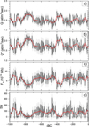 |
Fig. 2. Results of successive steps (Sect. 3.1) in the SN reconstructions. Panel a: 14C production rate Q. Panel b: Production rate Q* reduced to the present-day conditions. Panel c: Open solar flux Fo. Panel d: SN. For all panels, the black lines, grey shading, and red lines depict the mean annual reconstructed values, the 1σ uncertainties, and the 22-year smoothed curve (see Sect. 4), respectively. All data shown here are digitally available at the CDS. |
Step 2 reduces the radiocarbon production rates Q computed in Step 1 to the modern conditions (VDM = 7.75 ⋅ 1022 A m2) as Q*. This was done using the algorithm described by Usoskin et al. (2021, see Fig. 3 therein). For each ensemble realisation i, one VDM model was randomly chosen from the five models shown in Figure 1b. The same VDM was applied to all years within the ith realisation. The ensemble statistic of the Q* series is shown in Figure 2b. The evolution of the plotted Q* looks similar to that of Q, but has slightly higher values because the modern VDM value is longer and has a different long-term trend.
Step 3 computes the open solar flux Fo from the production rate Q*. Following Usoskin et al. (2021), we used the physics-based model
where F is in 1014 Wb, Q0 = 2.5 at/cm2/s, σF = 0.9 ⋅ 1014 Wb is the uncertainty of the conversion of the production rate into open flux (see details in Usoskin et al. 2021), and R is similar to that in Equation (2). The reconstructed open flux Fo is shown in Figure 2c.
The final step 4 converts the open solar flux Fo into the SN using an empirical algorithm developed by Usoskin et al. (2021). The SNi, j, for the ith ensemble realisation and jth year is calculated as

where g is the functional defined by Eq. (7) in Usoskin et al. (2021), σSN = 8 is the conversion uncertainty, and R is similar to that in other steps. The individual ensemble SN reconstructions are exemplified in Figure 3 for the period of 240–140 BC. The individual SN values vary, as indicated by the vertical extent of the grey region, but the cycles are defined robustly. The final reconstructed SN is shown in Figure 2d and is analysed in Sect. 4. Because the SN computation requires knowledge of the open flux for two years ahead, the reconstructed SN stops in 7 BC.
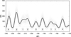 |
Fig. 3. Individual ensemble SN reconstructions (100 realizations; grey curves) along with the average curve (black) for the period of 240–140 BC, which includes cycles with a quality flag between 1 and 5 as indicated by the boxed numbers at the bottom of the panel (see Sect. 4.3 and Table 1). |
We note that the forward relation between SN and Fo is physical (Solanki et al. 2002b; Vieira & Solanki 2010) and was used in the model called Spectral and Total Irradiance Reconstruction over the telescopic period (SATIRE-T) for reconstructing the solar irradiance (Krivova et al. 2010, 2021; Wu et al. 2018a). For the inverted relation considered in step 4, we used an empirical approach as described in Usoskin et al. (2021), however.
3.2. Correction for the ESPE of 664 BC
Radiocarbon is generally produced by GCRs in the Earth’s atmosphere, and it thus serves as a proxy for geomagnetic and solar activity variability. In rare cases (roughly once in 1.5 millennia), it can also be produced by ESPEs (Miyake et al. 2020; Brehm et al. 2022; Usoskin et al. 2023). While the production is short (it occurs within a few months; Uusitalo et al. 2018), its effect can be visible in Δ14C for several years because of the “memory” of the carbon cycle that is caused by the large carbon pool in the atmosphere. This is in a continuous exchange with other carbon reservoirs such as the biosphere, the ocean, and soils. These events are sometimes called Miyake events. They can significantly distort the SN reconstruction and must be carefully removed. The first millennium BC we studied contains one such ESPE that occurred in about 664 BC (Park et al. 2017). It was found to be somewhat weaker than the ESPE of 774 AD, but had a similar shape of the energetic particle spectrum (O’Hare et al. 2019; Brehm et al. 2022; Koldobskiy et al. 2022).
The ESPEs are characterised by short-duration and spatially inhomogeneous radiocarbon production in the polar stratosphere. Consequently, the standard box carbon-cycle model is poorly suited for these events because they explicitly assume a full mixing of 14C within the atmospheric reservoirs. To properly consider this uneven production, we developed a new 3D time-dependent atmospheric transport model called Solar Climate Ozone Links (SOCOL):14C-Ex (Uusitalo et al. 2024; Golubenko et al. 2025). The model has been tested (Golubenko et al. 2025) with the ESPE of 774 AD and reproduced the Δ14C values in central Europe, where the data we used here were obtained.
For this study, we arbitrarily scaled the modelled time profile of Δ14C for the ESPE 774 AD down by a factor of 0.3 and added it to the linear trend to match the measured Δ14C values for the period 664–625 BC, as shown in Figure 4a. This profile was removed from the raw Δ14C data, and we considered the residual (shown in Figure 4b) as the corrected signal. The resulting SN reconstruction is shown in Figure 4c as the red curve. The solar cycles are clearly well preserved, including the cycle close to the maximum of which the ESPE of 664 BC took place. The reconstruction without the ESPE correction (dashed blue curve) appears to be smeared for the period around 660 BC, but it exhibits three slightly enhanced cycles after this. The grey curve depicts the SN reconstruction based on the production rate Q detrended for the ESPE of 664 BC as provided by Brehm et al. (2025). Figure 4c shows that the cycle around 665 BC is restored, but the four subsequent cycles are distorted.
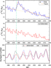 |
Fig. 4. Correction for the ESPE of 664 BC. Panel a: Raw annual Δ14C data (blue curve) for the period 685–600 BC (Brehm et al. 2025) along with the ESPE-modelled time profile (red curve; see Sect. 3.2) superimposed onto a linear trend caused by the slow relaxation of the 14C atmospheric concentration after the previous grand minimum (dotted orange line). Panel b: Detrended Δ14C data after the removal of the ESPE profile. Panel c: Reconstructed SN based on the raw (dotted blue curve) and detrended (red curve) Δ14C data, along with the SN based on the 14C production rate Q from Brehm et al. (2025). The vertical dashed green line denotes 664 BC when the ESPE took place. |
We note that the ESPE occurrence year, 664 BC, corresponds to the maximum phase of the corrected reconstructed SN cycle. It falls on a deep dip, however, when the ESPE effect is not removed.
3.3. Uncertainties
There are three independent sources of uncertainty in the SN reconstruction. They are detailed below.
(i) The Δ14C uncertainties are typically ≈1.7‰ (Brehm et al. 2025) and include the measurement errors and the dispersion of the 14C content between samples. These uncertainties are random and independent between individual points and were modelled in the MC way so that the value of each annual data point was taken according to Eq. (2). This uncertainty directly translates into the uncertainty on Q and propagates further to the SN.
(ii) The geomagnetic VDM uncertainties are related to the possible error of compiling the VDM value from local paleo- or archeo-magnetic measurements that are spatially and temporarily unevenly distributed (e.g., Genevey et al. 2008; Panovska et al. 2019). These uncertainties are not random, but can be treated as systematic or model uncertainties. They enter the reconstruction chain at step (2) and reduce the 14C production rate Q to the present-day conditions, Q*. They propagate further to the SN. For each reconstruction realisation, we randomly chose one of five available VDM models, as described in Sect. 3.1.
(iii) The model uncertainties of the conversion of Q* into the SN values (Usoskin et al. 2021) are involved in steps 3 and 4. They were modelled as described in Sect. 3.1 (see Eqs. (3) and (4)).
The uncertainties on the final SN-value reconstruction related to these sources are shown in Figure 5 along with the total uncertainty estimated using the full MC procedure by tracing only one uncertainty source at a time and switching the others off (see Sect. 3.1). The uncertainties related to the measurement errors dominate and range from 15–70 in SN. The geomagnetic uncertainties are smaller and range from 5–40 in SN. The model uncertainties are modest. They range from 12–20 in SN. Because the individual sources are independent of each other, the total uncertainty is close to the sum of the orthogonally summed individual sources and ranges from 20 SN during solar minima to 80 for the high-cycle maxima.
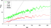 |
Fig. 5. Different types of uncertainties of the SN reconstruction as a function of the SN values estimated with the MC method. The dashed black, red, and blue curves represent the 1σ uncertainties in the SN value for the Δ14C, geomagnetic VDM, and the model uncertainties, respectively (see text). The green curve depicts the total uncertainty. The dashed black line denotes the diagonal. |
Because these uncertainties include both the random and systematic uncertainties, they do not present the range of the interannual SN variability, but rather the uncertainties on the overall SN level. The dates of the solar cycle minima and maxima are not expected to be affected by systematic uncertainties.
Another source of uncertainty that was not considered above arises from the choice of smoothing applied to Δ14C in step 1. Figure 6 shows a single realisation (using the same geomagnetic VDM and Ri, j = 0 for all steps) of our reconstructed SN using four different values for the low-pass-filter normalised frequency parameter wc. Higher smoothing values (wc ≥ 0.2) result in a noisier reconstruction and blur the individual solar cycles. Conversely, lower values (wc < 0.1) tend to suppress the amplitude of the solar cycles. The choice of this parameter involves some arbitrariness. We therefore chose our adopted value (wc = 0.17) to be optimal for a clear identification of the solar cycles. The exact choice of the frequency does not affect the overall level of the reconstructed activity.
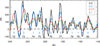 |
Fig. 6. Effect of the applied Δ14C smoothing parameter on our SN reconstruction. The values of the smoothing normalised frequency wc are indicated in the legend. The lower part of the figure shows the numbering of each solar cycle in black, along with the assigned quality flags in blue (see Sect. 4.3 and Table 1). The horizontal dashed line marks the SN = 0 line. |
4. Results
4.1. Reconstructing the sunspot number
The reconstructed annual sunspot numbers SN1 (in the definition of ISN-v2 – Clette & Lefèvre 2016) are shown in Figure 7 along with the total uncertainties and the smoothed series. The smoothing was performed using the 22-year low-pass singular spectrum analysis (SSA) method. For comparison, the decadal SN reconstruction based on a multi-proxy dataset (Wu et al. 2018b) is shown as the green curve. The smoothed SN we reconstructed agrees well with the decadal result by Wu et al. (2018b), except for the period before about 920 BC and two short periods at about 150 and 40 BC.
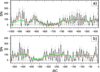 |
Fig. 7. Reconstructed sunspot numbers for 997–7 BC, shown in two panels for better visibility. The black curve, grey shaded area, and red curve depict the mean annual reconstructed SN, its 1σ (68%) confidence interval, and the 22-year smoothed evolution (see main text), respectively. These data are identical to those in Figure 2d. The green curve depicts the decadal SN values reconstructed from multi-proxy cosmogenic isotope data by Wu et al. (2018b) reduced to the ISN-v2 normalisation. The horizontal dashed line marks the SN = 0 line. |
The SN varies strongly from zero up to about 300. This is comparable to the SN range during the past 400 years. Two full grand minima are present in the reconstructed SN in about 800–700 BC and 400–330 BC (cf. Usoskin et al. 2007; Inceoglu et al. 2015). Additionally, two short Dalton-type minima can be seen in about 900 BC and 50 BC. The level of the cycles outside the grand minima is quite stable around 80–100 SN, except in the period about 950 BC, when it reaches about 150. This is comparable to the Modern grand maximum of the activity.
The distribution as a probability density function (PDF) of the 11-year-averaged reconstructed SNs is shown in Figure 8 for 100 random realisations of the SN series, that is, for about 9400 cycles. For each SN series realisation, we first smoothed it with an 11-year low-pass SSA filter and then took every tenth and eleventh value subsequently. This roughly represents the cycle-averaged SN values for a 10.5-year mean period, but does not require defining individual cycle lengths in each noisy realisation. The distribution is significantly bimodal, with a normal mode centred at an SN of about 70 (mean 68, standard deviation 51), and a grand-minimum mode with values of about zero (mean 3.3, standard deviation 3.6). This bimodality of the distribution is clearer when the distributions are produced separately for the grand minima periods (here set as 807–722 BC and 408–334 BC; see Table 1) and for the remaining cycles (Figure 8b). In particular, the grand minima periods result in a clearly skewed distribution, with a rather narrow peak around ⟨SN⟩ = 0. This confirms the paradigm that grand minima form a special mode in the operation of the solar dynamo, which is otherwise quite stable (e.g., Usoskin et al. 2014; Käpylä et al. 2016; Karak 2023). We note that the formally negative SN values, which sometimes appear around solar cycle minima, are consistent with zero within the uncertainties.
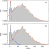 |
Fig. 8. Probability density function of the occurrence of the 11-year-average SN for 100 random realisations of the SN reconstructions (grey histogram). Panel a: Best-fit double Gaussian (μ1 = 3.3, σ1 = 3.6; μ2 = 68, σ2 = 51; red) and individual Gaussians (dashed blue). Panel b: Distributions of cycles that are defined to be part of a grand solar minimum (807–722 BC and 408–334 BC; see Table 1; blue) and the remaining cycles (orange). |
4.2. Periodicity
The SN variability is clearly dominated by the 11-year solar cycle, but a secular variability is also visible in Figure 7. Figure 9 shows the mean power spectrum of the reconstructed SN. The spectrum was computed with the fast Fourier transform (FFT) method with a Hanning window for 1000 SN reconstructions. The significance of the spectral peaks was checked against the auto-regressive AR1 noise (the autocorrelation coefficient with a one-year time shift, AR1 = 0.924), which is typical for auto-correlated datasets. Only one peak is clearly statistically significant (p < 0.05). This period range of this broad peak extends from 9.5 to 11 years, and its highest point corresponds to 10.45 years. This frequency corresponds to the averaged length of the 11-year cycles in the reconstructed series (see Sect. 4.3). Additionally, insignificant peaks are observed at 14.2 and 40–50, and a broad peak extends from 150–300 years. The latter peak likely corresponds to the Suess-de Vries cycle with a period of about 210 years, which manifests itself via the recurrence of grand minima (e.g., Usoskin et al. 2016). No power is found in the range corresponding to the centennial Gleissberg cycle with a period of 80–140 years (Gleissberg 1939).
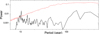 |
Fig. 9. Power spectrum (FFT, Hanning window) of the mean annual SN series averaged over 1000 reconstructions. The red line represents the 95% confidence level for the AR1 red noise (1000 realisations). Before the FFT, the series was standardised and zero-padded. |
The lack of significant stable periods beyond the Schwabe cycle range is expected since the SN series is non-stationary and not multi-harmonic (e.g., Biswas et al. 2023). Accordingly, some cycles may appear intermittently and/or with an unstable phase. The FFT does not work properly in a situation like this. Consequently, we also considered the wavelet power spectrum (using the tool by Grinsted et al. 2004) of the mean SN series, as shown in Figure 10. Here, again, only the Schwabe cycle appears to be statistically significant within a period range of 8–16 years, but it disappears during the grand minima. Some low power is seen in a period of about 50 years during the second half of the studied interval. A high power is found in a period of about 200 years (Suess-de Vries cycle), but it is not statistically significant because of the length of the dataset is insufficient.
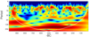 |
Fig. 10. Wavelet spectrum (Morlet basis, k = 6) of the reconstructed annual mean SN series. The black-contoured areas represent the significant spectral power (p < 0.05 against the AR1 red noise). The white line bounds the cone of influence below which the results are unreliable. |
4.3. Solar cycles
Based on the annual SN reconstruction shown in Figure 7, we assessed the dates of all solar cycle minima and consequently identified individual solar cycles. The identified cycles are collected in Table 1, which lists 93 full cycles between 991 and 10 BC. This yields an average length of these solar cycles of about 10.5 years, which corresponds to the main peak in the FFT power spectrum. It is also close to the mean length of directly observed sunspot cycles since 1700, which is about 10.7 years. About half of the cycles are clearly defined, and the others are distorted or hard to identify clearly. Accordingly, it cannot be excluded that a few cycles may be over- or under-counted.
In Table 1 we provide a quality flag q that specifies the quality of the reconstructed cycles (cf. Usoskin et al. 2021). The flag q is defined as follows:
-
0
The cycle cannot be unambiguously identified or its strength is indistinguishable from zero at the 1σ level. We found 13 such cycles.
-
1
The cycle is strongly distorted, at least one of its ends cannot be defined, or its strength is indistinguishable from zero at the 2σ level. We found 17 such cycles.
-
2
The cycle can be approximately identified, but either its shape or level is distorted or its strength is indistinguishable from zero at the 3σ level. We found 19 such cycles.
-
3
The cycle is defined reasonably well with a somewhat unclear SN near the cycle minimum or maximum, or with some caveats, for instance, a short data gap. We found 21 such cycles.
-
4
The cycle is well defined and has a somewhat unclear amplitude. We found 14 such cycles.
-
5
The cycle is clear in shape and amplitude. We found 9 such cycles.
Figures 3 and 6 illustrate cycles with different quality flags from q = 1 (e.g., about 170–160 BC) to q = 5 (e.g., 250–240 BC). We note that the dates of the solar cycle minimum are defined with an accuracy of one year for the high-quality cycles (q = 4–5) and an accuracy of a few years for moderate-quality cycles (q = 3), and it is defined rather poorly for low-quality cycles (q < 2).
Solar cycle 32 (671–656 BC) is well shaped, and the year of the ESPE corresponds to the maximum phase of the solar cycle. However, this association ought to be taken with a caveat because the exact shape of cycle 32 might be affected by the removal of the ESPE. Accordingly, we set its quality-flag value q to 2 in the final SN reconstruction because of the uncertainties in the correction for the 664 BC ESPE.
This means that 44 cycles are well or reasonably well defined (q = 3–5), 36 are poorly defined (q = 1–2), and 13 can only be guessed at. All cycles during the grand minima of activity have q values of 0 or 1. There is some subjectivity in the assignment of the exact value of q. For instance, cycle 80 is assigned q = 4 because both its neighbouring cycles are poorly defined or undefined, which might affect its minimum dates, while cycles 76 and 77, which look similar in quality, are assigned q = 5 because at least one of their neighbours is well defined.
The cycle length, defined between the consecutive cycle minima, is shown in Figure 11. It ranges between 6–17 years for all cycles, but is more confined for moderate- (q ≥ 3) and high-quality cycles (q ≥ 4) at 9–14 and 10–13 years, respectively. The average cycle length for high-quality cycles is 10.9 years.
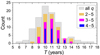 |
Fig. 11. Histogram of the min-to-min cycle lengths T for all cycles (grey shaded bars) and different values of the quality flag q as indicated in the legend. |
We also examined whether empirical rules related to solar cycles can be confirmed or ruled out for the first millennium BC. The relation between the cycle length T and the strength, which is quantified as the solar cycle averaged SN, ⟨SN⟩, for high-quality cycles (q = 4–5) is shown in Figure 12. They are anti-correlated at a significant level (p = 0.036, the linear Pearson correlation coefficient is r = 0.38), with the linear regression being

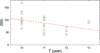 |
Fig. 12. Relation of the cycle-average SN value ⟨SN⟩ and the cycle length T for high-quality cycles (q ≥ 4). The dashed red line depicts the linear regression ⟨SN⟩= − 12.41 ⋅ T + 224 (Pearson linear correlation coefficient r = 0.38 ± 0.17, p = 0.037). |
which implies that stronger cycles tend to be shorter. This relation is similar to the empirical Waldmeier rule, which says that stronger cycles have shorter ascending phases (Hathaway 2015), but it is sometimes used in a simplified form that relates the cycle strength to its length. Because there are only a few subsequent high-quality cycles, the higher anti-correlation between the length and strength of subsequent cycles (Solanki et al. 2002a) cannot be verified. Unfortunately, the uncertainties on the dates of the cycle minima and maxima prevent us from drawing any conclusion about the validity of the original Waldmeier rule in the reconstruction series. Other empirical rules such as the Gnevyshev-Ohl rule of solar cycle pairing cannot be verified either.
5. Summary and conclusions
We presented the first annually resolved reconstruction of SNs for the first millennium BC. The reconstruction was made with the method developed by Usoskin et al. (2021) applied to newly published Δ14C measurements covering the period 1000–2 BC (Brehm et al. 2025). Our new reconstruction strongly agrees with previous decadal-resolution reconstructions (Wu et al. 2018b), but it tends to yield higher values during the period 1000–920 BC.
Our analysis identified 93 complete solar cycles over this period, with a mean cycle length of approximately 10.5 years. Twenty-three of these cycles are well defined, 21 are reasonably well defined, and the remainder are more uncertain. The total SN cycle statistic currently includes about 200 individual cycles, of which only 36 are based on directly observed sunspots. The others are based on high-precision 14C data as in Usoskin et al. (2021) and here. While our reconstruction occasionally produced negative SN, these values are statistically consistent with zero within their uncertainties.
The first millennium BC includes two grand minima (about 807–721 BC and 403–335 BC) and two short Dalton-type minima (about 900 BC and 50 BC). When examining the distribution of cycle amplitudes, we find that grand minima form a distinct mode of solar activity. This is consistent with previous findings (e.g. Usoskin et al. 2021) for the last millennium.
There was an ESPE during this period in about 664 BC. These events affect the measured 14C production and can distort the apparent shape of solar cycles in our reconstruction. To account for this, we applied corrections to the Δ14C data based on results with the 3D time-dependent atmospheric transport model SOCOL (Golubenko et al. 2025). After the correction, the data suggest that this event occurred around the maximum of a moderate solar activity cycle.
We find a strong quasi-periodic variability corresponding to the 11-year solar cycle, but no significant power for longer periodicities. Our reconstruction also reproduced the well-established empirical relation between cycle length and amplitude, albeit with considerable scatter.
This work provides unique insights into the solar cycles during the first millennium BC and is essential for studies of the solar dynamo and irradiance reconstructions.
Data availability
The reconstructed values are available at the CDS via anonymous ftp to cdsarc.cds.unistra.fr (130.79.128.5) or via https://cdsarc.cds.unistra.fr/viz-bin/cat/J/A+A/698/A182
Acknowledgments
We are grateful to Monika Korte for a very useful discussion on the archeo/paleo-magnetic models for the past millennium BC. This project has received funding from the European Research Council (ERC) under the European Union’s Horizon 2020 research and innovation programme (grant agreement No. 101097844 – project WINSUN). Partial support from the Research Council of Finland (RCF, project 354280) is acknowledged. This study has made use of NASA’s Astrophysics Data System (ADS; https://ui.adsabs.harvard. edu/) Bibliographic Services.
References
- Beer, J., McCracken, K., & von Steiger, R. 2012, Cosmogenic Radionuclides: Theory and Applications in the Terrestrial and Space Environments (Berlin: Springer) [Google Scholar]
- Biswas, A., Karak, B., Usoskin, I., & Weisshaar, E. 2023, Space Sci. Rev., 219, 19 [NASA ADS] [CrossRef] [Google Scholar]
- Brehm, N., Bayliss, A., Christl, M., et al. 2021, Nat. Geosci., 14, 10 [Google Scholar]
- Brehm, N., Christl, M., Knowles, T. D. J., et al. 2022, Nat. Commun., 13, 1196 [NASA ADS] [CrossRef] [Google Scholar]
- Brehm, N., Pearson, C., Christl, M., et al. 2025, Nat. Commun., 16, 406 [Google Scholar]
- Büntgen, U., Wacker, L., Galvan, J., et al. 2018, Nat. Commun., 9, 3605 [Google Scholar]
- Charbonneau, P. 2020, Liv. Rev. Solar Phys., 17, 4 [Google Scholar]
- Clette, F., & Lefèvre, L. 2016, Sol. Phys., 291, 2629 [Google Scholar]
- Clette, F., Lefèvre, L., Chatzistergos, T., et al. 2023, Sol. Phys., 298, 44 [NASA ADS] [CrossRef] [Google Scholar]
- Cliver, E. W., Schrijver, C. J., Shibata, K., & Usoskin, I. G. 2022, Liv. Rev. Solar Phys., 19, 2 [Google Scholar]
- Eddy, J. 1976, Science, 192, 1189 [Google Scholar]
- Fahrni, S., Southon, J., Fuller, B., et al. 2020, Radiocarbon, 62, 919 [Google Scholar]
- Genevey, A., Gallet, Y., Constable, C. G., Korte, M., & Hulot, G. 2008, Geochem., Geophys., Geosyst., 9, Q04038 [Google Scholar]
- Gleissberg, W. 1939, The Observatory, 62, 158 [NASA ADS] [Google Scholar]
- Golubenko, K., Usoskin, I., Rozanov, E., & Bard, E. 2025, Earth Planet. Sci. Lett., 661, 119383 [Google Scholar]
- Grinsted, A., Moore, J. C., & Jevrejeva, S. 2004, Nonlin. Processes Geophys., 11, 561 [NASA ADS] [CrossRef] [Google Scholar]
- Güttler, D., Adolphi, F., Beer, J., et al. 2015, Earth Planet. Sci. Lett., 411, 290 [Google Scholar]
- Hathaway, D. H. 2015, Liv. Rev. Sol. Phys., 12, 4 [Google Scholar]
- Heaton, T., Bard, E., Bayliss, A., et al. 2024, Nature, 633, 306 [Google Scholar]
- Inceoglu, F., Simoniello, R., Knudsen, V. F., et al. 2015, A&A, 577, A20 [CrossRef] [EDP Sciences] [Google Scholar]
- Käpylä, M. J., Käpylä, P. J., Olspert, N., et al. 2016, A&A, 589, A56 [NASA ADS] [CrossRef] [EDP Sciences] [Google Scholar]
- Karak, B. 2023, Liv. Rev. Solar Phys., 20, 3 [Google Scholar]
- Knudsen, M. F., Riisager, P., Donadini, F., et al. 2008, Earth Planet. Sci. Lett., 272, 319 [CrossRef] [Google Scholar]
- Koldobskiy, S. A., Usoskin, I., & Kovaltsov, G. 2022, J. Geophys. Res. Space Phys., 127, e2021JA029919 [CrossRef] [Google Scholar]
- Korte, M., Brown, M. C., Panovska, S., & Wardinski, I. 2019, Front. Earth Sci., 7, 86 [Google Scholar]
- Krivova, N. A., Vieira, L. E. A., & Solanki, S. K. 2010, J. Geophys. Res., 115, A12112 [Google Scholar]
- Krivova, N. A., Solanki, S. K., Hofer, B., et al. 2021, A&A, 650, A70 [NASA ADS] [CrossRef] [EDP Sciences] [Google Scholar]
- Miyake, F., Usoskin, I., & Poluianov, S. (eds.) 2020, Extreme Solar Particle Storms: The Hostile Sun (Bristol, UK: IOP Publishing) [Google Scholar]
- Nilsson, A., Suttie, N., Stoner, J., & Muscheler, R. 2022, Procs. Nat. Acad. Sci., 119, e2200749119 [Google Scholar]
- Nilsson, A., Nguyen, L., Panovska, S., et al. 2024, Nat. Geosci., 17, 654 [Google Scholar]
- O’Hare, P., Mekhaldi, F., Adolphi, F., et al. 2019, Proc. Nat. Acad. Sci., 116, 5961 [Google Scholar]
- Panovska, S., Korte, M., & Constable, C. G. 2019, Rev. Geophys., 57, 1289 [Google Scholar]
- Park, J., Southon, J., Fahrni, S., Creasman, P. P., & Mewaldt, R. 2017, Radiocarbon, 59, 1147 [CrossRef] [Google Scholar]
- Parker, E. 1955, ApJ, 122, 293 [Google Scholar]
- Pavón-Carrasco, F. J., Osete, M. L., Torta, J. M., & De Santis, A. 2014, Earth Planet. Sci. Lett., 388, 98 [Google Scholar]
- Schanner, M., Korte, M., & Holschneider, M. 2022, J. Geophys. Res. (Solid Earth), 127, e2021JB023166 [Google Scholar]
- Snowball, I., & Muscheler, R. 2007, Holocene, 17, 851 [NASA ADS] [CrossRef] [Google Scholar]
- Solanki, S., Krivova, N., Schüssler, M., & Fligge, M. 2002a, A&A, 396, 1029 [NASA ADS] [CrossRef] [EDP Sciences] [Google Scholar]
- Solanki, S., Schüssler, M., & Fligge, M. 2002b, A&A, 383, 706 [NASA ADS] [CrossRef] [EDP Sciences] [Google Scholar]
- Solanki, S. K., Usoskin, I. G., Kromer, B., Schüssler, M., & Beer, J. 2004, Nature, 431, 1084 [Google Scholar]
- Steinhilber, F., Abreu, J., Beer, J., et al. 2012, Proc. Nat. Acad. Sci. USA, 109, 5967 [Google Scholar]
- Usoskin, I. G. 2023, Liv. Rev. Solar Phys., 20, 2 [Google Scholar]
- Usoskin, I. G., Solanki, S. K., Schüssler, M., Mursula, K., & Alanko, K. 2003, Phys. Rev. Lett., 91, 211101 [Google Scholar]
- Usoskin, I. G., Solanki, S. K., & Kovaltsov, G. A. 2007, A&A, 471, 301 [CrossRef] [EDP Sciences] [Google Scholar]
- Usoskin, I. G., Hulot, G., Gallet, Y., et al. 2014, A&A, 562, L10 [NASA ADS] [CrossRef] [EDP Sciences] [Google Scholar]
- Usoskin, I. G., Gallet, Y., Lopes, F., Kovaltsov, G. A., & Hulot, G. 2016, A&A, 587, A150 [CrossRef] [EDP Sciences] [Google Scholar]
- Usoskin, I. G., Solanki, S. K., Krivova, N., et al. 2021, A&A, 649, A141 [EDP Sciences] [Google Scholar]
- Usoskin, I., Miyake, F., Baroni, M., et al. 2023, Space Sci. Rev., 219, 73 [Google Scholar]
- Uusitalo, J., Arppe, L., Hackman, T., et al. 2018, Nat. Commun., 9, 3495 [Google Scholar]
- Uusitalo, J., Golubenko, K., Arppe, L., et al. 2024, Geophys. Res. Lett., 51, e2023GL106632 [Google Scholar]
- Vaquero, J. M., Kovaltsov, G. A., Usoskin, I. G., Carrasco, V. M. S., & Gallego, M. C. 2015, A&A, 577, A71 [CrossRef] [EDP Sciences] [Google Scholar]
- Vaquero, J., Svalgaard, L., Carrasco, V., et al. 2016, Sol. Phys., 291, 3061 [Google Scholar]
- Vieira, L. E. A., & Solanki, S. K. 2010, A&A, 509, A100 [NASA ADS] [CrossRef] [EDP Sciences] [Google Scholar]
- Wu, C.-J., Krivova, N. A., Solanki, S. K., & Usoskin, I. G. 2018a, A&A, 620, A120 [NASA ADS] [CrossRef] [EDP Sciences] [Google Scholar]
- Wu, C. J., Usoskin, I. G., Krivova, N., et al. 2018b, A&A, 615, A93 [NASA ADS] [CrossRef] [EDP Sciences] [Google Scholar]
All Tables
All Figures
|
Fig. 1. Data for the first millennium BC used here. Panel a: Raw Δ14C data along with the 1σ uncertainties (indicated by the black line and grey shaded band, respectively; Brehm et al. 2025). The red arrow indicates the signature of the ESPE at about 664 BC. Panel b: Paleo- and archaeo-magnetic reconstructions of the virtual dipole moment (VDM), according to 1 Usoskin et al. (2016), 2 Knudsen et al. (2008), 3 Pavón-Carrasco et al. (2014), 4 Schanner et al. (2022), and 5 Nilsson et al. (2022). |
| In the text | |
|
Fig. 2. Results of successive steps (Sect. 3.1) in the SN reconstructions. Panel a: 14C production rate Q. Panel b: Production rate Q* reduced to the present-day conditions. Panel c: Open solar flux Fo. Panel d: SN. For all panels, the black lines, grey shading, and red lines depict the mean annual reconstructed values, the 1σ uncertainties, and the 22-year smoothed curve (see Sect. 4), respectively. All data shown here are digitally available at the CDS. |
| In the text | |
|
Fig. 3. Individual ensemble SN reconstructions (100 realizations; grey curves) along with the average curve (black) for the period of 240–140 BC, which includes cycles with a quality flag between 1 and 5 as indicated by the boxed numbers at the bottom of the panel (see Sect. 4.3 and Table 1). |
| In the text | |
|
Fig. 4. Correction for the ESPE of 664 BC. Panel a: Raw annual Δ14C data (blue curve) for the period 685–600 BC (Brehm et al. 2025) along with the ESPE-modelled time profile (red curve; see Sect. 3.2) superimposed onto a linear trend caused by the slow relaxation of the 14C atmospheric concentration after the previous grand minimum (dotted orange line). Panel b: Detrended Δ14C data after the removal of the ESPE profile. Panel c: Reconstructed SN based on the raw (dotted blue curve) and detrended (red curve) Δ14C data, along with the SN based on the 14C production rate Q from Brehm et al. (2025). The vertical dashed green line denotes 664 BC when the ESPE took place. |
| In the text | |
|
Fig. 5. Different types of uncertainties of the SN reconstruction as a function of the SN values estimated with the MC method. The dashed black, red, and blue curves represent the 1σ uncertainties in the SN value for the Δ14C, geomagnetic VDM, and the model uncertainties, respectively (see text). The green curve depicts the total uncertainty. The dashed black line denotes the diagonal. |
| In the text | |
|
Fig. 6. Effect of the applied Δ14C smoothing parameter on our SN reconstruction. The values of the smoothing normalised frequency wc are indicated in the legend. The lower part of the figure shows the numbering of each solar cycle in black, along with the assigned quality flags in blue (see Sect. 4.3 and Table 1). The horizontal dashed line marks the SN = 0 line. |
| In the text | |
|
Fig. 7. Reconstructed sunspot numbers for 997–7 BC, shown in two panels for better visibility. The black curve, grey shaded area, and red curve depict the mean annual reconstructed SN, its 1σ (68%) confidence interval, and the 22-year smoothed evolution (see main text), respectively. These data are identical to those in Figure 2d. The green curve depicts the decadal SN values reconstructed from multi-proxy cosmogenic isotope data by Wu et al. (2018b) reduced to the ISN-v2 normalisation. The horizontal dashed line marks the SN = 0 line. |
| In the text | |
|
Fig. 8. Probability density function of the occurrence of the 11-year-average SN for 100 random realisations of the SN reconstructions (grey histogram). Panel a: Best-fit double Gaussian (μ1 = 3.3, σ1 = 3.6; μ2 = 68, σ2 = 51; red) and individual Gaussians (dashed blue). Panel b: Distributions of cycles that are defined to be part of a grand solar minimum (807–722 BC and 408–334 BC; see Table 1; blue) and the remaining cycles (orange). |
| In the text | |
|
Fig. 9. Power spectrum (FFT, Hanning window) of the mean annual SN series averaged over 1000 reconstructions. The red line represents the 95% confidence level for the AR1 red noise (1000 realisations). Before the FFT, the series was standardised and zero-padded. |
| In the text | |
|
Fig. 10. Wavelet spectrum (Morlet basis, k = 6) of the reconstructed annual mean SN series. The black-contoured areas represent the significant spectral power (p < 0.05 against the AR1 red noise). The white line bounds the cone of influence below which the results are unreliable. |
| In the text | |
|
Fig. 11. Histogram of the min-to-min cycle lengths T for all cycles (grey shaded bars) and different values of the quality flag q as indicated in the legend. |
| In the text | |
|
Fig. 12. Relation of the cycle-average SN value ⟨SN⟩ and the cycle length T for high-quality cycles (q ≥ 4). The dashed red line depicts the linear regression ⟨SN⟩= − 12.41 ⋅ T + 224 (Pearson linear correlation coefficient r = 0.38 ± 0.17, p = 0.037). |
| In the text | |
Current usage metrics show cumulative count of Article Views (full-text article views including HTML views, PDF and ePub downloads, according to the available data) and Abstracts Views on Vision4Press platform.
Data correspond to usage on the plateform after 2015. The current usage metrics is available 48-96 hours after online publication and is updated daily on week days.
Initial download of the metrics may take a while.