| Issue |
A&A
Volume 698, June 2025
|
|
|---|---|---|
| Article Number | A184 | |
| Number of page(s) | 11 | |
| Section | Numerical methods and codes | |
| DOI | https://doi.org/10.1051/0004-6361/202554703 | |
| Published online | 13 June 2025 | |
ThermoONet: Deep learning-based small-body thermophysical network
Applications to modeling the water activity of comets
1
School of Astronomy and Space Science, Nanjing University,
Nanjing
210023,
China
2
Key Laboratory of Modern Astronomy and Astrophysics in Ministry of Education, Nanjing University,
Nanjing
210023,
China
3
Shanghai Astronomical Observatory, Chinese Academy of Sciences,
Shanghai
200030,
China
★ Corresponding authors: This email address is being protected from spambots. You need JavaScript enabled to view it.
; This email address is being protected from spambots. You need JavaScript enabled to view it.
Received:
22
March
2025
Accepted:
29
April
2025
Abstract
Cometary activity is a compelling subject of study, with thermophysical models playing a pivotal role in its understanding. However, traditional numerical solutions for small body thermophysical models are computationally intensive, posing challenges for investigations requiring high-resolution or repetitive modeling. To address this limitation, we employed a machine learning approach to develop ThermoONet – a neural network designed to predict the temperature and water ice sublimation flux of comets. Performance évaluations indicate that ThermoONet achieves a low average error in subsurface temperature of approximately 2% relative to the numerical simulation, while reducing the computational time by nearly six orders of magnitude. We applied ThermoONet to model the water activity of comets 67P/Churyumov-Gerasimenko and 21P/Giacobini-Zinner. By successfully fitting the water production rate curves of these comets, obtained by the Rosetta mission and the SOHO telescope, respectively, we have been able to demonstrate the network's effectiveness and efficiency. Furthermore, when combined with a global optimization algorithm, ThermoONet proves capable of retrieving the physical properties of target bodies.
Key words: methods: numerical / comets: general
© The Authors 2025
 Open Access article, published by EDP Sciences, under the terms of the Creative Commons Attribution License (https://creativecommons.org/licenses/by/4.0), which permits unrestricted use, distribution, and reproduction in any medium, provided the original work is properly cited.
This article is published in open access under the Subscribe to Open model. This email address is being protected from spambots. You need JavaScript enabled to view it. to support open access publication.
1 Introduction
Comets are active, small Solar System bodies. When approaching the Sun, their nuclei get heated up and volatile ices within them sublimate, dragging dust particles alongside to form detectable coma and tails (Whipple 1950). The activity of comets is an intriguing topic, as it provides insights into the formation and evolution of comets, such as the cyclical variations in the relative abundance of water ice keeping the comet “alive” (De Sanctis et al. 2015; Shi et al. 2018), while heat transport and ice sublimation help reflect the properties of the uppermost layer of cometary nucleus (Gulkis et al. 2015) and seasonal effects of ice sublimation induce various topographical changes (El-Maarry et al. 2015; Tang et al. 2025). Their activity can also help us understand the possibility that comets could have delivered water to Earth (Mandt et al. 2024).
Within ∼3 au, water vapor is the predominant species in outgassing (Hässig et al. 2015; Läuter et al. 2020). The water production rate and the dust production rate are primary indicators for characterizing cometary activity and its variations. The modeling of water and dust production requires us to simulate the thermophysical processes, taking into account the orbit and the shape of the nucleus, as well as its various physical properties. There are variations in the thermophysical models for different aims (Watson et al. 1963; Cowan & A'Hearn 1979; Weissman & Kieffer 1981). They have been applied in quantitative analysis of the impact of parameters on water ice activity (Marshall et al. 2019), as well as investigating mechanisms behind the disruption of a cometary nucleus (Steckloff et al. 2015). For interpreting observational data, more realistic thermophysical models are required, such as the inversion of 67P's physical properties from non-gravitational force caused by outgassing (Davidsson & Gutiérrez 2005), the evolution of morphology of the nucleus influenced by the insolation-induced activity (Keller et al. 2015a; Groussin et al. 2025), interpretation of the measured water production (Hu et al. 2017; Blum et al. 2017; Attree et al. 2019), and the explanation of distinct activity phenomena, such as shortlived outbursts from fractured terrains (Skorov et al. 2016). To further improve the model fidelity, it is necessary to consider additional complex physical mechanisms, such as the behavior of volatile transport in the nucleus given rise by its porosity, the deposition of gas on dust particles, and so on (De Sanctis et al. 1999; Davidsson & Skorov 2002; Gortsas et al. 2011; González et al. 2014; Hu & Shi 2021).
Traditionally, thermophysical models are realized by numerical treatment based on the finite-difference technique, such as the Crank-Nicolson method utilized by Hu et al. (2017). However, it usually requires relatively high computation cost due to the iterative calculations performed on a large time-space grids, leading to limited efficiency in related studies and posing challenges for practical implementation. Firstly, the inverse extraction of physical parameters automatically from observational data is a difficult problem, typically, the forward trial-and-error method is utilized (Keller et al. 2015a; Hu et al. 2017; Attree et al. 2019). In addition, Combi et al. (2019, 2021b, 2023) have been continuously updating the water production rate curves of numerous comets, although directly solving the thermal models through numerical simulation to analyze these data is clearly a highly challenging task. The orbital evolution of the comet influenced by non-gravitational acceleration from sublimation (Davidsson & Gutiérrez 2005; Attree et al. 2019; Jewitt et al. 2020), as well as the changes in its spin state due to the non-gravitational torque (Keller et al. 2015b; Attree et al. 2024), are both complex topics in the context of forward evolution and fitting the observational data as well. If the thermophysical model is embedded within a complex physical process as a sub-mechanism, such as the shape evolution (Zhao et al. 2021) and coma formation (Shi et al. 2018), conducting large-scale or high-resolution studies is also challenging.
In our previous work, we addressed similar issues in the thermophysical modeling for asteroids by introducing deep learning techniques (Zhao et al. 2024). Here, we have applied a similar concept to develop a deep learning-based approach for the comets that can efficiently solve the thermophysical process and produce the water production rate.
This paper covers: (i) how the deep learning model can be applied to model the thermal physics of comets; (ii) whether the deep learning model can serve as a unified model for simulating the water activity of the comets in large parameter spaces; and (iii) how the deep learning model can be utilized in the analysis of real comet data.
2 Thermophysical model and water activity
In this work, we adopted the so called “dust mantle model,” in which a dry dust layer is present at the surface of the nucleus over the dust-ice mixture and the water ice sublimation occurs at the boundary between the mantle and the ice front (Hu et al. 2017, and references therein).
2.1 Dust mantle model
The nucleus is regarded as a polyhedron consisting of triangular facets. For each facet, neglecting the changes in thermal properties due to the gas from ice sublimation filling the porosity of the nucleus, the 1D heat conduction equation can be expressed as follows:
 (1)
where ρ, C, and κ correspond to the density, specific heat capacity, and thermal conductivity, respectively. They are assumed to be different constants in dry dust mantle and dust-ice mixture, denoted as ρd, Cd, κd and ρm, Cm, κm. In fact, ρmCm, κm can be expressed in terms of ρd, Cd, κd and ρi, Ci, κi of the pure water ice (Davidsson & Skorov 2002; Davidsson & Gutiérrez 2005):
(1)
where ρ, C, and κ correspond to the density, specific heat capacity, and thermal conductivity, respectively. They are assumed to be different constants in dry dust mantle and dust-ice mixture, denoted as ρd, Cd, κd and ρm, Cm, κm. In fact, ρmCm, κm can be expressed in terms of ρd, Cd, κd and ρi, Ci, κi of the pure water ice (Davidsson & Skorov 2002; Davidsson & Gutiérrez 2005):
 (2)
where f is the icy area fraction and h is the Hertz factor, dependent on the morphological structure of the medium and is generally regarded as a free parameter (Davidsson & Skorov 2002).
(2)
where f is the icy area fraction and h is the Hertz factor, dependent on the morphological structure of the medium and is generally regarded as a free parameter (Davidsson & Skorov 2002).
The surface boundary condition of the dust mantle derived from conservation of energy is expressed as (Kührt & Keller 1994; Lagerros 1996):
 (3)
where ∊ is the emissivity, σ is the Stefan-Boltzmann constant. (1 - AB) SψFθ describes the radiation flux received by the facet, AB is the Bond albedo, s indicates whether the facet is illuminated by the Sun, considering the horizon shadows and projected shadows, ψ represents the cosine function of the solar elevation angle, and Fθ is the incident solar radiation flux determined by Fθ = Sθ/r2. Here, r is the heliocentric distance of the asteroid and Sθ is the solar constant.
(3)
where ∊ is the emissivity, σ is the Stefan-Boltzmann constant. (1 - AB) SψFθ describes the radiation flux received by the facet, AB is the Bond albedo, s indicates whether the facet is illuminated by the Sun, considering the horizon shadows and projected shadows, ψ represents the cosine function of the solar elevation angle, and Fθ is the incident solar radiation flux determined by Fθ = Sθ/r2. Here, r is the heliocentric distance of the asteroid and Sθ is the solar constant.
It is necessary to introduce an additional boundary condition at the interface between the dust mantle and dust-ice mixture, due to the energy consumption caused by water ice sublimation. Assuming the thickness of the dust mantle is X, the condition can be expressed as (Kührt & Keller 1994; Hu et al. 2017):
 (4)
then, l is the latent heat of water ice, Z(X) is the mass flux of sublimation determined by (Hu et al. 2017):
(4)
then, l is the latent heat of water ice, Z(X) is the mass flux of sublimation determined by (Hu et al. 2017):
 (5)
where
(5)
where
 (6)
(6)
This equation comes from the Hertz-Knudsen formula, describing the sublimation flux from the surface of pure solid ice into vacuum (Kossacki et al. 1999; Gundlach et al. 2011); m̄ is the mass of a water molecules and kB is the Boltzmann constant; PV(T) is the saturation vapor pressure; α(T) is the sublimation coefficient, representing the reduction in sublimation flux due to the reattachment of gas molecules to the ice surface after impacting with each other. They are respectively evaluated as (Panale & Salvail 1984; Mauersberger & Krankowsky 2003; Gundlach et al. 2011):
 (7)
with constants a, b, c0, c1, c2, and c3 taking the values of 3.23×10¹² Pa, 6134.6 K, 0.146, 0.854, 57.78, and 11 580 K.
(7)
with constants a, b, c0, c1, c2, and c3 taking the values of 3.23×10¹² Pa, 6134.6 K, 0.146, 0.854, 57.78, and 11 580 K.
The parameter Ψ in Eq. (5) represents the reduction factor in the sublimation flux from the bare icy surface, accounting for the permeability of the mantle to gas flow. It is given by the expression 1/(1 + pH) (Gundlach et al. 2011; Hu et al. 2017), where p is a constant and H = X/d, with d denoting the diameter of the spherical dust aggregates in the dust mantle (Skorov & Blum 2012). We take p = 0.14 and d = 1 mm in this work, similarly to the approach taken by Hu et al. (2017). Furthermore, f in Eq. (5) is used to approximate the reduction in sublimation flux from the pure ice caused by the presence of mixed dust, as the Hertz-Knudsen formula is derived for pure ice (Crifo 1997).
The last boundary condition describes the invariability of temperature at infinitely large depth,
 (8)
(8)
2.2 Normalization of thermophysical model
A direct application of deep learning methods to the model described above presents several challenges: (1) the parameters have a broad dynamic range, leading to the fact that the resulting temperature distribution could span over a wide numerical range; (2) The model is influenced by the rotational velocity of comet, which is not explicitly represented in the established equations. Instead, it is implicitly embedded in the time-dependent function Sψ and the time steps used in the subsequent numerical simulations. Therefore, normalization becomes particularly crucial in this context.
We denote the rotational angular velocity as ω and introduce the following normalized variables (Lagerros 1996),
 (9)
where lsd and lsm are the skin depth of the dust mantle and the dust-ice mixture, Te is the theoretical maximum surface temperature at the heliocentric distance, r, called the characteristic temperature, given by:
(9)
where lsd and lsm are the skin depth of the dust mantle and the dust-ice mixture, Te is the theoretical maximum surface temperature at the heliocentric distance, r, called the characteristic temperature, given by:
![Mathematical equation: l_{sd} = \sqrt{\frac{\kappa_d}{\rho_d C_d \omega}},\;l_{sm} = \sqrt{\frac{\kappa_m}{\rho_m C_m \omega}},\;T_e = \sqrt[4]{\frac{(1-A_B)F_\odot}{\epsilon \sigma}},](/articles/aa/full_html/2025/06/aa54703-25/aa54703-25-eq10.png) (10)
the heat conduction equation Eq. (1) and three boundary conditions Eq. (3), Eq. (4), and Eq. (8) can then be normalized as:
(10)
the heat conduction equation Eq. (1) and three boundary conditions Eq. (3), Eq. (4), and Eq. (8) can then be normalized as:
 (11)
where Φd and Φm are the thermal parameters (Spencer et al. 1989) of the dust mantle and dust-ice mixture, defined by
(11)
where Φd and Φm are the thermal parameters (Spencer et al. 1989) of the dust mantle and dust-ice mixture, defined by
 (12)
(12)
Here, E(t̄) is the radiation flux rescaled in the range [0, 2π] for variables t̄ and [0, 1] for E. Then, Z̄(X̄) = Z(X)/(1 - AB)FΘ is the sublimation flux after variation.
It is evident that the radiation flux and the derived temperature can be successfully rescaled in the range of [0, 1], with all the physical parameters explicitly represented in the mathematical expression of the equations. This transformation can significantly enhance the efficiency and ease of dataset creation for deep learning. For instance, when studying different comets, the original model for the radiation flux functions leads to varying domains of definition due to differences in rotational velocities. Additionally, the range of values fluctuates with variable parameters such as the Bond albedo, AB, and heliocentric distance, r. This variability complicates the construction of a comprehensive set of radiation flux functions. However, the normalized model can effectively address this issue through the parameter extraction.
Excluding the radiation flux, we have identified and summarized all the independent parameters that influence the equations:
 (13)
(13)
In the following discussion, we treat all these parameters as variable within a physically reasonable range in order to obtain a generalized model.
2.3 Numerical treatment
The radiation flux needs to be calculated before solving the equations. It is a periodic function about time, determined by the angle between the normal vector of the surface element and the solar direction, incorporating both the horizon and projected shadows. The calculation method is consistent with our previous work for asteroids (secondary radiation and self-heating are not considered in this work), as described in Sect. 2.1.2 of Zhao et al. (2024). It is worth noting that the radiation flux used to train the network should be randomly generated, which will be detailed in Sect. 3, while the illumination and shadow mentioned here are solely specific to real-world situations.
The backward finite difference method is utilized to solve the partial differential equations, considering its computational efficiency. First, we divided the continuous variables into a set of space-time grids, where the i-th grid of depth is denoted by iΔx̄ and the j-th grid of time is denoted as jΔt̄. As a result, the heat conduction equation is discretized into
 (14)
(14)
The thickness of the dust mantle is much smaller than that of the dust-ice mixture. To improve computational efficiency while ensuring accuracy, different spatial step sizes are applied in two layers, with a smaller step size Δxd = 1 mm for the dust mantle and a larger one Δxm = 1 cm for the dust-ice mixture. Then, Δx̄d and Δx̄m can be obtained by dividing Δxd and Δxm by the skin depth, lsd, lsm. The time step is taken as Δt̄ = 2π/1200. We denote the temperature at the interface between the two layers as Tm,j, then the three boundary conditions are expressed in the finite difference scheme as follows:
 (15)
(15)
The surface temperature, T0, j, and the interface temperature, Tm,j, can be determined from the known T1,j, Tm-1, j, Tm+1,j by taking advantage of Newton-Raphson iterative algorithm to solve the boundary conditions.
The overall temperature needed to exhibit a stable and static distribution due to the rotation of the comet. After one complete spin of the nucleus, the temperature should be invariant at the subsolar point, which holds at all depths. This static condition is used as a convergence criterion for the iteration. In this work, the criterion is for the mean absolute error of the normalized temperature between iterations to be below 1 × 10⁻⁴.
2.4 Water activity
The water activity of the comet is effectively represented by the sublimation flux in the model. The global total outgassing flux of water from the comet nucleus is the integral of the sublimation flux over the entire surface. In the polyhedral shape model, this can be expressed as follows (Hu et al. 2017):
 (16)
where Zk indicates the sublimation flux of k-th facet and its area is denoted as Sk. Furthermore, we calculated the global water production rate by averaging the global outgassing flux of water over one rotational period, which quantifies the number of water molecules produced per second, given by (Hu et al. 2017) where P is the rotational period.
(16)
where Zk indicates the sublimation flux of k-th facet and its area is denoted as Sk. Furthermore, we calculated the global water production rate by averaging the global outgassing flux of water over one rotational period, which quantifies the number of water molecules produced per second, given by (Hu et al. 2017) where P is the rotational period.
3 ThermoONet
In Zhao et al. (2024), we showed that many factors in a thermophysical model makes the equation-driven deep learning models such as physics-informed neural networks (PINNs; Raissi et al. 2019) unsuitable, despite their successful application in solving ordinary differential equations (ODEs) and partial differential equations (PDEs; Cai et al. 2020; Zobeiry & Humfeld 2021; He et al. 2021; Martin & Schaub 2022a,b; Mathews & Thompson 2023; Laghi et al. 2023). Therefore, for the asteroid thermophysical modeling, we adopted deep operator neural network (DeepONet) with strong generalization abilities (Lu et al. 2021; Garg et al. 2022; He et al. 2023; Branca & Pallottini 2024). Such a network is well suited for handling problems with variable boundary conditions. Following the same consideration, we continue to utilize DeepONet for the development of ThermoONet in this work.
The surface of an asteroid is treated as a layer of dust, whose temperature is influenced primarily by the radiation flux and the thermal parameter (a total of two independent parameters). However, for comets, the distinct physical properties of the dust-ice mixture layer in contrast to the dust mantle, along with the phase transitions of water ice, necessitate a more complex selection of parameters to describe the thermophysical process. Consequently, we identified a total of eight independent parameters (Eq. (13)). In this work, we modified the structure of the neural network to address the high dimensionality of the parameters. Furthermore, we manually optimized the distribution of the training dataset, based on the relative impact of different parameters on the results. The specific methods are introduced in detail below.
3.1 Architecture of the neural network
The principles and structure of DeepONet are explained in detail in Lu et al. (2021). Here, we just provide a brief summary. The core idea is to utilize a neural network to map the different variables from the partial differential equations into a common mathematical space for processing. The network that maps the parameters or functions of the equations is referred to as the branch network, while the network that maps the independent variables is called the trunk network. If we denote the parameters or functions as independent variables, such as as u, y, these two mapping relationships can be expressed as u → G(u) and y → G(u)(y), where G is called the operator.
In the thermophysical modeling of cometary systems, the operator mapping process involves the radiation flux function, E(t̄), and eight characteristic parameters from Eq. (13), with the depth and time serving as independent variables. A DeepONet architecture could theoretically be constructed with branch networks encoding radiation flux function and parameters, such as trunk networks handling independent variables. The large number of parameters renders the training of an accurate neural network particularly challenging. This necessitates a simplification of the network architecture through problem-specific adaptations. Theoretically the sublimation flux fundamentally depends on the temperature at the dust mantle-and-dust-ice mixture interface. This physical understanding enables significant architectural simplification by reducing the network output to this subsurface temperature. Consequently, the trunk network becomes redundant and can be eliminated, with the branch network outputs directly providing the temperature predictions. For the comprehensive modeling of non-gravitational effects induced by sublimation processes, additional consideration must be given to the surface temperature of the dust mantle, which should be incorporated as another output. This dual-temperature approach enables the simultaneous prediction of both the subsurface temperature governing sublimation dynamics and the surface temperature, which is essential for calculating the velocity of the gas (detailed analyses of these effects are provided in Attree et al. 2019 and Jewitt et al. 2020).
In the asteroid network, we model the thermal behavior of the asteroid using two separate branch networks: one for encoding the radiation flux function and the other for encoding the thermal parameter (Zhao et al. 2024). The treatment of generating random radiation flux functions can be directly adapted to the comet model (see Sect. 3.2 for more about the dataset). However, the comet model introduces a larger number of independent parameters exhibiting heterogeneous sensitivity to the solutions of the model, so direct adoption of the parameter encoding scheme for asteroids proves ineffective. A single branch network collectively encoding all parameters can reduce sensitivity to each individual parameter, especially for those parameters significantly influencing the results. Conversely, constructing separate branch networks for individual parameters would result in excessive computational memory allocation and time cost. To resolve this challenge, we propose a parameter grouping method based on sensitivity analysis. Parameters governing the thermal processes are partitioned into two distinct categories: high-sensitivity and moderate-sensitivity parameters. Each category is encoded through dedicated branch network, achieving an optimal balance between parameter sensitivity and computational efficiency.
The schematic architecture of the neural network adapted for this work is shown in Fig. 1, where the branch networks are presented in Fig. 2. Parameter group1 consists of the high-sensitivity parameters, p1, which exhibit a dominant influence over system behavior (more details are shown in Appendix A), while parameter group2 consists of the remaining parameters. The neural network encodes these grouped parameters through dedicated branch networks (branch net1 and branch net2), followed by a Hadamard product operation between their respective outputs. This combined tensor undergoes transformation through an attention mechanism layer, designed to amplify the features through adaptive weight allocation (Vaswani et al. 2017; Woo et al. 2018; Wang et al. 2020). Notably, each branch network incorporates internal attention mechanisms to perform hierarchical feature enhancement. The target subsurface temperature is derived from a averaging operation to the Hadamard product between the amplified features and branch net3 output.
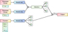 |
Fig. 1 Architecture of ThermoONet. The network consists of three branch networks with distinct inputs, parameter group, p1, p2-8, and the radiation flux function, E, where E is presented as some discrete locations with m elements sampled on [t̄1,t̄2,...,t̄m]. A layer incorporating the attention mechanism processes the Hadamard product of the outputs from branch net1 and branch net2. The resulting output from this layer [ |
![Mathematical equation: $[b_1^1,b_2^1,...,b_p^1]$](/articles/aa/full_html/2025/06/aa54703-25/aa54703-25-eq17.png)
![Mathematical equation: $[b_1^2,b_2^2,...,b_p^2]$](/articles/aa/full_html/2025/06/aa54703-25/aa54703-25-eq18.png)
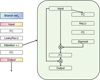 |
Fig. 2 Detailed architectures of branch netn and attention mechanism, where FC is the full connected layer. The input of branch netn experiences the initial feature extraction through a FC layer and then carries out the feature amplification by attention mechanism, where i represents the layer number. 3, 6, and 6 layers are respectively used in branch networks from net1 to net3. |
3.2 Dataset and training
The neural network developed in this work focuses on the diurnal water ice activity. Seasonal variations in thermal conditions are reflected through variations in insolation.
As mentioned above, the neural network will be trained with a nine-dimensional parameter space, comprising the scalar parameters, p1-p8, and one functional input, E, representing the normalized diurnal insolation curve. To ensure that ThermoONet is able to efficiently generalize across different cometary environments, we should design a training dataset comprised of a broad, diverse selection of diurnal radiation flux curves.
For training the asteroid network, we produced a dataset with random pairs of the radiation flux function, E, and the thermal parameter, Φd (Zhao et al. 2024). The corresponding temperatures were calculated by the numerical simulation. Random functions are generated by the mean-zero Gaussian random field (GRF; Lu et al. 2021), then rescaled in the range [0, 1] through the sigmoid function 1/(1 + e−(x+d)), where d represents the translation distance along the y axis in order to ensure the completeness of the function space (Zhao et al. 2024). For the network used in this study, the training process employs a modified stochastic sampling framework, adapted for cometary thermophysical model requirements. The only difference is that all eight parameters undergo a simultaneous joint randomization to maintain proper parameter covariance structures. A special treatment can be implemented for high-sensitivity parameter p1 through a stratified sampling strategy; p1 is randomly generated within different value ranges, with a similar number in each range. This balanced multi-range generation mechanism, grounded in prior knowledge of the nonlinear dominance of p1, ensures that the network effectively captures the substantial influence of various ranges on the resulting temperature. In the practical training process, we generated a dataset with 36 000 sets of data.
The loss function is the mean square error (MSE) between the temperature calculated with numerical simulation and the output from the neural network and the adaptive moment estimation method (Adam) is used as the optimization algorithm. Just as in the training process of the asteroid network in Zhao et al. (2024), the learning rate decay approach was utilized to mitigate issues related to wide oscillations of the loss function and slow convergence.
We called the trained neural network ThermoONet, designed on the basis of the core principles of DeepONet and specifically tailored for cometary thermophysical modeling.
4 Results
The cost of computation time and the level of accuracy are used to assess the performance of ThermoONet.
4.1 Computational cost
We compared the computational time consumed by three approaches: ThermoONet with GPU, ThermoONet with CPU, and a traditional numerical simulation, for calculating the global ice front temperature distribution of a spherical nucleus with varying number of facets. It is worth mentioning that dataset construction required approximately 6 hours, while the neural network training process was completed within 20 minutes. Once trained, the network is ready for immediate application and does not require further adjustment, so we only need to analyze the inference time of the network. The ThermoONet calculations were carried out on both GPU and CPU for over 20 times to get an estimate on the uncertainty. The time consumption of the numerical simulation is evaluated by multiplying the average time cost per facet (calculated based on the temperature of a large number of facets) by the total number of facets. All of the computations were performed on a personal computer1 and under the environment of Python 3.8. Our results indicate, as shown in Fig. 3, that:
Calculations using ThermoONet are approximately six orders of magnitude faster than the numerical simulation.
Computational time costs by numerical and CPU-based ThermoONet increase almost linearly with number of facets, while the computation cost by GPU-based ThermoONet stays almost constant against an increasing number of facets. When we need to calculate a large number of global temperature distributions, it is worth noting that the vectorized operations can be used next to ensure that the computation time does not increase linearly with the number of facets.
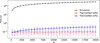 |
Fig. 3 Comparison of computational cost between ThermoONet and traditional numerical simulation for the shape models with varying number of facets. The error bars represent the maximum and minimum time costs in the repeated calculation for more than 20 times. |
4.2 Accuracy assessment
First, we used a spherical comet to assess the accuracy of temperature predictions with varying obliquity, β, (the angle between the spin axis and the normal vector of the orbital plane) and heliocentric distance, r. We also investigated how the errors change with different key model parameters such as the thickness of the dust mantle, X, and icy area fraction, f , where fixed parameters are listed in Table 1. We measure the mean absolute percentage error (MAPE) of temperature between the neural network and numerical simulation, denoted as MAPE (T).
Figure 4 shows the results. The overall error in temperature fluctuates as the radiation flux function or parameters change. With the inclusion of more parameters, the error inevitably increases compared to that of the deep learning model for asteroids (Zhao et al. 2024). However, it is still maintained at a reasonably low level, with a maximum below 4% and an average around 2%. We notice that the error does not show significant correlation with varying heliocentric distances, which confirms the effectiveness of the specially designed training dataset.
As shown in Eqs. (5)-(7), the sublimation flux of water ice exhibits an exponential relationship with the temperature, meaning that any error in temperature has an even more significant impact on the calculated sublimation flux. Moreover, given that many cometary nucleus show a concave shape, the projected shadows between facets complicate the radiation flux function. This presents a great challenge for the generalization of the neural network, which is even more severe than in the case of asteroid (Zhao et al. 2024). To validate the generalization capability of ThermoONet, it is applied to a real comet with irregular shape. In practice, we take comet 67P as the example and simulate its temperature with a shape model of 2868 facets (Jorda et al. 2016). Ephemerides of 67P is retrieved using Rosetta SPICE kernels (Acton 1996; ESA SPICE Service 2017). We evaluated both the temperature and water production rate at different orbital phases by comparing them with the results from numerical solutions (see Fig. 5). We also examined the temperature distributions at three specific orbital locations before, near, and after the perihelion (Fig. 6). The other parameters are the same as in Table 1.
The average temperature errors are about 2.5% and the global water production rates from two methods exhibit the same trend. The average relative errors are respectively 5.04% for (X = 5mm, f = 1%), 19.25% for (X = 5mm, f = 10%), and 10.26% for (X = 10 mm, f = 1%). The patterns of the error distribution shown in Fig. 5 suggest that the temperature error is the smallest in the high-temperature region, typically below 3 K. The primary source of error lies in the mid-temperature regions. However, only a few facets exhibit errors exceeding 10 K.
Fixed parameters in the error analysis.
5 Application to the interpretation of water production rate
Interpreting the water production rate as a function of the heliocentric distance using thermophysical models has been an intriguing topic in cometary science as it helps us understand the nature of cometary activity (Keller et al. 2015a; Hu et al. 2017; Attree et al. 2019; Marshall et al. 2019; Skorov et al. 2020). It is a time-consuming process to calculate the water production rate curve (hereafter, the 'water curve') using traditional numerical simulation, which requires computations of the global temperature distribution at different orbital phases. Thus, it needs to be recalculated whenever the parameters are adjusted. Due to the large number of physical parameters involved, previous studies often fix certain parameters to some typical values, leaving only afew that are adjustable. When fitting the observational data, itis difficult to take advantage of the automated algorithms to extract parameters from the observational data; thus, the parameters are typically determined through empirical trial-and-error testing.
Generating water curves with ThermoONet is efficient, thereby enabling the application of global optimization algorithms, such as genetic algorithm (GA), particle swarm optimization (PSO), simulated annealing (SA), and so on, to find the best-fitting parameters. To do so, we implemented ThermoONet to calculate the water curve in three steps:
A lookup table was generated by calculating illumination and shadows under varying solar positions, incorporating the shape and rotational state of the comet. This is achieved through Möller-Trumbore algorithms and interpolation algorithms.
Eight scalar parameters are computed based on the physical properties of the comet and orbital ephemerides, the radiation flux for each facet then is retrieved from the precomputed lookup table.
The derived nine-dimensional parameters serve as input to ThermoONet, which outputs the sub-surface temperature at the ice front of each facet. The results subsequently drive the calculation of water ice sublimation rates and associated activity levels.
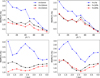 |
Fig. 4 Differences in the output subsurface temperature between ThermoONet and numerical simulation as functions of obliquity, β, and heliocentric distance, r. The left panels present the error functions for different thicknesses of dust mantle, with the blue, black, and red lines, representing 5 mm, 10 mm, and 15 mm respectively. The right panels illustrate the error functions for varying icy area fractions, with the blue, black, and red lines respectively corresponding to 1%, 10%, and 20%. The panels are fixed to r = 2 au for the top and β = 0° for the bottom, along with f = 10% for the left panels and X = 10 mm for the right panels. For the settings of other parameters, we refer to Table 1. |
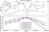 |
Fig. 5 Differences in global water production rate derived from Ther-moONet and the numerical simulation at different orbital phases of comet 67P. The top panel is the temperature calculation errors, where the black line was derived with X = 5 mm, f = 1%, and the red line with X = 10 mm, f = 1%, the blue line with X = 5 mm, and f = 10%. The asterisks denote specific examples of temperature distributions shown in Fig. 6. The bottom panel is the water production rate, where the real lines stand for the results from ThermoONet, while the circles refer to the numerical solutions, with the same parameters as in the top one. |
5.1 Fitting the water curve of 67P
We combine ThermoONet with SA to fit the observed water curve of comet 67P from Läuter et al. (2020), the shape model with 23 788 facets is used (Jorda et al. 2016). We chose five parameters to be fitted, including the thickness of the dust mantle, X, the icy area fraction, f , the product between the density of the dust mantle, ρd, and the specific heat capacity, Cd, the heat conductivity of the dust mantle, κd, and the dust-ice mixture, κm. The initial values of the five parameters are selected as in Table 2 and the corresponding water curve is generated by applying ThermoONet at every observation time. The loss function is MAPE between the predicted results and the average observed data and SA is applied to search for the preliminary optimal parameter combination that minimizes MAPE. Finally, a batch gradient descent (BGD) was utilized to refine the parameters, converging to a solution that further reduces the loss function. The best-fitting water curve is shown in Fig. 7 and the optimized parameter combination is shown in Table 2.
The overall fitting performance is satisfactory with MAPE = 37.08%, capturing the asymmetrical trend before and after perihelion. A slight underestimation is observed near the perihelion, which is consistent with the finding in Hu et al. (2017). This phenomenon may be explained by several factors, including the varying levels of activity across different regions of 67P (Attree et al. 2019), the gradual exposure of water ice as the comet approaches perihelion (Fornasier et al. 2016; Filacchione et al. 2020), and the temperature-dependent changes in thermal conductivity (Skorov et al. 2020). It is worth mentioning that the advantage of ThermoONet in computation efficiency could be of help in assessing aforementioned mechanisms.
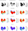 |
Fig. 6 Sub-surface temperature distribution of comet 67P modeled by ThermoONet and the numerical simulation at three specific positions marked by asterisks in the top panel of Fig. 5. The top row shows the normalized radiation flux and the second to fourth rows show the results calculated with ThermoONet, the numerical simulation, and the differences between them. |
Initial values and the results derived from SA and BGD for the variable parameters in fitting the water curve of 67P.
5.2 Fitting the water curve of 21P
There is a growing database of water curves of different types of comets retrieved using observations by solar observatories Combi et al. (2019, 2021b, 2023). Most of these comets still lack well-defined parameters such as size, shape, rotation characteristics, and thermophysical parameters. It could prove difficult for traditional numerical simulations to fit these data by searching a large parameter space. However, by combining trial-and-error testing with ThermoONet, exploring a large parameter space becomes feasible. We take comet 21P as an example to demonstrate the application of the trial-and-error testing. The water curve of 21P is significantly different from that of 67P, remaining essentially flat before perihelion and exhibiting an obvious decline after perihelion (see more in Combi et al. 2021a). A preliminary consideration is that the solar illumination area of 21P gradually decreases during the observation period, which could be the combined effect of its shape and the orientation of its spin axis. This was described in Marshall et al. (2019). We can iteratively adjust the parameters based on trial-and-error results by taking advantage of ThermoONet.
Figure 8 shows preliminary fitting results. The fixed parameters are ∊ = 1, ω = 1.74 × 10⁻⁴ rad s−1 (the rotation period is uncertain with a wide range from 9.5 to 19 h (Leibowitz & Brosch 1986; Moulane et al. 2020). The parameters included in the fitting are shown in Table 3. The test shapes are respectively sphere with ax = ay = az = 3.5 km, biaxial ellipsoid with ax = 2ay = 2az = 5.2 km, and triaxial ellipsoid ax = 2ay = 4az = 5.2 km. As shown in Fig. 8, the evolutionary trend of the triaxial ellipsoid better matches the observational data, confirming our previous hypothesis regarding the solar illumination area, meaning that the farther the comet is before the perihelion, the larger the region with the higher temperature.
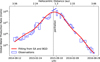 |
Fig. 7 Fitting the global water production rate of 67P as a function of time. The blue rectangles represent the observation data from Läuter et al. (2020), and the red line corresponds to the best fit curve achieved by combining ThermoONet with the optimization algorithm. The black dashed line indicates the epoch of the perihelion. A detailed description of the observation data and sources thereof can be found in Läuter et al. (2020). |
6 Conclusion
In this work, we have developed ThermoONet, a DeepONet-based neural network for modeling cometary activity. Due to the high-dimensional parameter space in cometary thermophysical model, we tailored the architecture of DeepONet by removing the trunk network and trained it specifically for the target temperature. With the solar flux as input, ThermoONet predicts the subsurface temperatures and water production rate. By taking advantage of the generalization ability of DeepONet, ThermoONet could be used in modeling comets with varying physical parameters and shapes.
We conducted a comprehensive evaluation of the network's performance, including its computation time, accuracy, and generalization ability. The results show that ThermoONet deployed on GPU has the highest efficiency and generates the global sublimation flux approximately six orders of magnitude faster than using numerical simulation. The accuracy of ThermoONet varies with parameters, with an average of around 2%. Ther-moONet can be successfully applied to irregular comets as exemplified by comet 67P, with the water production rate curve closely matching the numerical simulation, demonstrating a strong generalization ability and practicability.
We tested the capability of ThermoONet in computationally demanding tasks by fitting global water production rate curves of comets using global optimization algorithms. By applying a simulated annealing, we successfully fit the observed water production rate curve of comet 67P derived with the Rosetta mission data and obtained a set of optimized physical parameters of 67P. Additionally, we fit the water curve of comet 21P to demonstrate the capability of combining ThermoONet with trial-and-error testing. Although limited knowledge is available for 21P, we managed to reconstruct the unique trend observed in its water production rate by adjusting the shape, rotation, and thermal parameters.
We anticipate a broad range of application for ThermoONet in various research topics concerning small body activities. In addition to its application to large-scale and high-resolution data analysis, it can also serve as an efficient model that can be embedded into more complex physical systems.
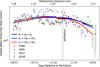 |
Fig. 8 Fitting the global water production rate of 21P as a function of days from perihelion by applying ThermoONet to different shapes. The black line corresponds to a sphere model, the blue line is a ellipsoid model with ax = 2ay = 2az and the red line is a ellipsoid with ax = 2ay = 4az. Other parameters are as stated in Table 3. The scatter points with different colors and shapes represent observational data at different apparitions (Combi et al. 2019), where purple circles from 1998, blue triangles from 2005, green squares from 2012, and black asterisks from 2018. The detailed description about the observation data and sources thereof can be found in Combi et al. (2019). |
Parameters for fitting the water curve of 21P.
Acknowledgements
The authors thank Prof. Groussin for the insightful review comments that helped to significantly improve the manuscript. The authors thank Dr. Xuanyu Hu for extensive discussions on the thermophysical modeling for comets. XS thanks members of the ISSI International Team “Timing and Processes of Planetesimal Formation and Evolution” for inspirational discussions. This work is financially supported by the National Natural Science Foundation of China (No. 12233003 and 12073011) and the China Manned Space Program with grant no. CMS-CSST-2025-A16.
Appendix A Parameter sensitivity
We conducted the parameter sensitivity analysis using the controlled variable approach with a fixed radiation flux as an example. When modifying a single parameter, the remaining parameters maintain their reference values, as specified in Table A.1. Here, the rotational angular velocity p5 is represented as the rotation period. Figure A.1 shows the resultant variations in temperature curves induced by alterations of different parameters; p1 primarily influences the value range of temperature distributions, whereas the remaining parameters affect the shape of temperature curves within this established range.
Parameters and their reference values used in the parameter sensitivity analysis.
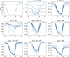 |
Fig. A.1 Comparative analysis of parameter sensitivity. The first panel depicts the selected example radiation flux, followed by eight panels illustrating different temperature curves under varying values of the eight distinct parameters. The titles of these panels show the variation ranges with units as the same as Table A.1 and the curves with darker hues correspond to larger values of parameters. |
References
- Acton, C. H. 1996, Planet. Space Sci., 44, 65 [Google Scholar]
- Attree, N., Jorda, L., Groussin, O., et al. 2019, A&A, 630, A18 [NASA ADS] [CrossRef] [EDP Sciences] [Google Scholar]
- Attree, N., Gutiérrez, P., Groussin, O., et al. 2024, A&A, 690, A82 [NASA ADS] [CrossRef] [EDP Sciences] [Google Scholar]
- Blum, J., Gundlach, B., Krause, M., et al. 2017, MNRAS, 469, S755 [Google Scholar]
- Branca, L., & Pallottini, A. 2024, A&A, 684, A203 [NASA ADS] [CrossRef] [EDP Sciences] [Google Scholar]
- Cai, S., Wang, Z., Chryssostomidis, C., & Karniadakis, G. E. 2020, in ASME 2020 Fluids Engineering Division Summer Meeting collocated with the ASME 2020 Heat Transfer Summer Conference and the ASME 2020 18th International Conference on Nanochannels, Microchannels, and Minichannels 3: Computational Fluid Dynamics; Micro and Nano Fluid Dynamics, V003T05A054 [Google Scholar]
- Combi, M. R., Mäkinen, T. T., Bertaux, J. L., Quémerais, E., & Ferron, S. 2019, Icarus, 317, 610 [NASA ADS] [CrossRef] [Google Scholar]
- Combi, M. R., Mäkinen, T., Bertaux, J. L., et al. 2021a, Icarus, 357, 114242 [Google Scholar]
- Combi, M. R., Shou, Y., Mäkinen, T., et al. 2021b, Icarus, 365, 114509 [CrossRef] [Google Scholar]
- Combi, M. R., Mäkinen, T., Bertaux, J. L., Quémerais, E., & Ferron, S. 2023, Icarus, 398, 115543 [NASA ADS] [CrossRef] [Google Scholar]
- Cowan, J. J., & A'Hearn, M. F. 1979, Moon Planets, 21, 155 [NASA ADS] [CrossRef] [Google Scholar]
- Crifo, J. F. 1997, Icarus, 130, 549 [Google Scholar]
- Davidsson, Björn, J. R., & Skorov, Yuri, V. 2002, Icarus, 159, 239 [CrossRef] [Google Scholar]
- Davidsson, Björn, J. R., & Gutiérrez, Pedro, J. 2005, Icarus, 176, 453 [NASA ADS] [CrossRef] [Google Scholar]
- De Sanctis, M. C., Capaccioni, F., Capria, M. T., et al. 1999, PSS, 47, 855 [Google Scholar]
- De Sanctis, M. C., Capaccioni, F., Ciarniello, M., et al. 2015, Nature, 525, 500 [NASA ADS] [CrossRef] [Google Scholar]
- El-Maarry, M. R., Thomas, N., Gracia-Berná, A., et al. 2015, Geophys. Res. Lett., 42, 5170 [Google Scholar]
- ESA SPICE Service 2017, Operational SPICE Kernel Dataset [Google Scholar]
- Filacchione, G., Capaccioni, F., Ciarniello, M., et al. 2020, Nature, 578, 49 [NASA ADS] [CrossRef] [Google Scholar]
- Fornasier, S., Mottola, S., Keller, H. U., et al. 2016, Science, 354, 1566 [NASA ADS] [CrossRef] [Google Scholar]
- Garg, S., Gupta, H., & Chakraborty, S. 2022, Eng. Struct., 270 [Google Scholar]
- González, M., Gutiérrez, P. J., & Lara, L. M. 2014, A&A, 563, A98 [NASA ADS] [CrossRef] [EDP Sciences] [Google Scholar]
- Gortsas, N., Kührt, E., Motschmann, U., & Keller, H. U. 2011, Icarus, 212, 858 [Google Scholar]
- Groussin, O., Jorda, L., Attree, N., et al. 2025, A&A, 694, A21 [NASA ADS] [CrossRef] [EDP Sciences] [Google Scholar]
- Gulkis, S., Allen, M., von Allmen, P., et al. 2015, Science, 347, aaa0709 [Google Scholar]
- Gundlach, B., Skorov, Y., & Blum, J. 2011, Icarus, 213, 710 [Google Scholar]
- He, J. Y., Koric, S., Kushwaha, S., et al. 2023, Comput. Methods Appl. Mech. Eng., 415 [Google Scholar]
- He, Z. L., Ni, F. T., Wang, W. G., & Zhang, J. 2021, Mater. Today Commun., 28 [Google Scholar]
- Hu, X., & Shi, X. 2021, ApJ, 910, 10 [Google Scholar]
- Hu, X., Shi, X., Sierks, H., et al. 2017, MNRAS, 469, S295 [NASA ADS] [CrossRef] [Google Scholar]
- Hässig, M., Altwegg, K., Balsiger, H., et al. 2015, Science, 347, aaa0276 [Google Scholar]
- Jewitt, D., Kim, Y., Mutchler, M., et al. 2020, ApJ, 896, L39 [NASA ADS] [CrossRef] [Google Scholar]
- Jorda, L., Gaskell, R., Capanna, C., et al. 2016, Icarus, 277, 257 [Google Scholar]
- Keller, H. U., Mottola, S., Davidsson, B., et al. 2015a, A&A, 583, A34 [NASA ADS] [CrossRef] [EDP Sciences] [Google Scholar]
- Keller, H. U., Mottola, S., Skorov, Y., & Jorda, L. 2015b, A&A, 579, L5 [NASA ADS] [CrossRef] [EDP Sciences] [Google Scholar]
- Kossacki, K. J., Markiewicz, W. J., Skorov, Y., & Kömle, N. I. 1999, PSS, 47, 1521 [Google Scholar]
- Kührt, E., & Keller, H. U. 1994, Icarus, 109, 121 [Google Scholar]
- Lagerros, J. S. V. 1996, A&A, 310, 1011 [Google Scholar]
- Laghi, L., Schiassi, E., De, M., Furfaro, F. R., & Domiziano, M. 2023, Nucl. Sci. Eng., 197, 2373 [NASA ADS] [CrossRef] [Google Scholar]
- Läuter, M., Kramer, T., Rubin, M., & Altwegg, K. 2020, MNRAS, 498, 3995 [Google Scholar]
- Leibowitz, Elia, M., & Brosch, N. 1986, Icarus, 68, 430 [NASA ADS] [CrossRef] [Google Scholar]
- Lu, L., Jin, P., Pang, G., Zhang, Z., & Karniadakis, G. E. 2021, NAT MACH INTELL, 3, 218 [Google Scholar]
- Mandt, K. E., Lustig-Yaeger, J., Luspay-Kuti, A., et al. 2024, Sci. Adv., 10, eadp2191 [Google Scholar]
- Marshall, D., Rezac, L., Hartogh, P., Zhao, Y., & Attree, N. 2019, A&A, 623, A120 [NASA ADS] [CrossRef] [EDP Sciences] [Google Scholar]
- Martin, J., & Schaub, H. 2022a, CeMDA, 134, 46 [NASA ADS] [CrossRef] [Google Scholar]
- Martin, J., & Schaub, H. 2022b, CeMDA, 134, 13 [NASA ADS] [CrossRef] [Google Scholar]
- Mathews, N., & Thompson, B. 2023, Bull. AAS, 55 [Google Scholar]
- Mauersberger, K., & Krankowsky, D. 2003, GRL, 30 [CrossRef] [Google Scholar]
- Moulane, Y., Jehin, E., Rousselot, P., et al. 2020, A&A, 640, A54 [NASA ADS] [CrossRef] [EDP Sciences] [Google Scholar]
- Panale, Fraser, P., & Salvail, James, R. 1984, Icarus, 60, 476 [NASA ADS] [CrossRef] [Google Scholar]
- Raissi, M., Perdikaris, P., & Karniadakis, G. E. 2019, J. Comput. Phys., 378, 686 [NASA ADS] [CrossRef] [Google Scholar]
- Shi, X., Hu, X., Mottola, S., et al. 2018, Nat. Astron., 2, 562 [NASA ADS] [CrossRef] [Google Scholar]
- Skorov, Y., & Blum, J. 2012, Icarus, 221, 1 [Google Scholar]
- Skorov, Y., Keller, H. U., Mottola, S., & Hartogh, P. 2020, MNRAS, 494, 3310 [NASA ADS] [CrossRef] [Google Scholar]
- Skorov, Y. V., Rezac, L., Hartogh, P., Bazilevsky, A. T., & Keller, H. U. 2016, A&A, 593, A76 [NASA ADS] [CrossRef] [EDP Sciences] [Google Scholar]
- Spencer, John R., Lebofsky, Larry A., & Sykes, Mark V. 1989, Icarus, 78, 337 [CrossRef] [Google Scholar]
- Steckloff, J. K., Johnson, B. C., Bowling, T., et al. 2015, Icarus, 258, 430 [CrossRef] [Google Scholar]
- Tang, X., Shi X., & El-Maarry, M. R. 2025, ApJ, 979, 91 [Google Scholar]
- Vaswani, A., Shazeer, N., Parmar, N., et al. 2017, in Proceedings of the 31st International Conference on Neural Information Processing Systems, NIPS'17 (Red Hook, NY, USA: Curran Associates Inc.), 6000 [Google Scholar]
- Wang, Q., Wu, B., Zhu, P., et al. 2020, in 2020 IEEE/CVF Conference on Computer Vision and Pattern Recognition [Google Scholar]
- Watson, K., Murray, B. C., & Brown, H. 1963, Icarus, 1, 317 [Google Scholar]
- Weissman, P. R., & Kieffer, H. H. 1981, Icarus, 47, 302 [Google Scholar]
- Whipple, F. L. 1950, ApJ, 111, 375 [NASA ADS] [CrossRef] [Google Scholar]
- Woo, S. H., Park, J., Lee, J. Y., & Kweon, I. S. 2018, Comput. Vision ECCV 11211, 3 [Google Scholar]
- Zhao, Y., Rezac, L., Skorov, Y., et al. 2021, Nat. Astron., 5, 139 [Google Scholar]
- Zhao, S., Lei, H., & Shi, X. 2024, A&A, 691, A224 [NASA ADS] [CrossRef] [EDP Sciences] [Google Scholar]
- Zobeiry, N., & Humfeld, K. D. 2021, Eng. Appl. Artif. Intell., 101 [Google Scholar]
A laptop equipped with AMD Ryzen 9 6900HX with Radeon Graphics and NVIDIA GeForce RTX 3070Ti Laptop GPU.
All Tables
Initial values and the results derived from SA and BGD for the variable parameters in fitting the water curve of 67P.
Parameters and their reference values used in the parameter sensitivity analysis.
All Figures
|
Fig. 1 Architecture of ThermoONet. The network consists of three branch networks with distinct inputs, parameter group, p1, p2-8, and the radiation flux function, E, where E is presented as some discrete locations with m elements sampled on [t̄1,t̄2,...,t̄m]. A layer incorporating the attention mechanism processes the Hadamard product of the outputs from branch net1 and branch net2. The resulting output from this layer [ |
| In the text | |
|
Fig. 2 Detailed architectures of branch netn and attention mechanism, where FC is the full connected layer. The input of branch netn experiences the initial feature extraction through a FC layer and then carries out the feature amplification by attention mechanism, where i represents the layer number. 3, 6, and 6 layers are respectively used in branch networks from net1 to net3. |
| In the text | |
|
Fig. 3 Comparison of computational cost between ThermoONet and traditional numerical simulation for the shape models with varying number of facets. The error bars represent the maximum and minimum time costs in the repeated calculation for more than 20 times. |
| In the text | |
|
Fig. 4 Differences in the output subsurface temperature between ThermoONet and numerical simulation as functions of obliquity, β, and heliocentric distance, r. The left panels present the error functions for different thicknesses of dust mantle, with the blue, black, and red lines, representing 5 mm, 10 mm, and 15 mm respectively. The right panels illustrate the error functions for varying icy area fractions, with the blue, black, and red lines respectively corresponding to 1%, 10%, and 20%. The panels are fixed to r = 2 au for the top and β = 0° for the bottom, along with f = 10% for the left panels and X = 10 mm for the right panels. For the settings of other parameters, we refer to Table 1. |
| In the text | |
|
Fig. 5 Differences in global water production rate derived from Ther-moONet and the numerical simulation at different orbital phases of comet 67P. The top panel is the temperature calculation errors, where the black line was derived with X = 5 mm, f = 1%, and the red line with X = 10 mm, f = 1%, the blue line with X = 5 mm, and f = 10%. The asterisks denote specific examples of temperature distributions shown in Fig. 6. The bottom panel is the water production rate, where the real lines stand for the results from ThermoONet, while the circles refer to the numerical solutions, with the same parameters as in the top one. |
| In the text | |
|
Fig. 6 Sub-surface temperature distribution of comet 67P modeled by ThermoONet and the numerical simulation at three specific positions marked by asterisks in the top panel of Fig. 5. The top row shows the normalized radiation flux and the second to fourth rows show the results calculated with ThermoONet, the numerical simulation, and the differences between them. |
| In the text | |
|
Fig. 7 Fitting the global water production rate of 67P as a function of time. The blue rectangles represent the observation data from Läuter et al. (2020), and the red line corresponds to the best fit curve achieved by combining ThermoONet with the optimization algorithm. The black dashed line indicates the epoch of the perihelion. A detailed description of the observation data and sources thereof can be found in Läuter et al. (2020). |
| In the text | |
|
Fig. 8 Fitting the global water production rate of 21P as a function of days from perihelion by applying ThermoONet to different shapes. The black line corresponds to a sphere model, the blue line is a ellipsoid model with ax = 2ay = 2az and the red line is a ellipsoid with ax = 2ay = 4az. Other parameters are as stated in Table 3. The scatter points with different colors and shapes represent observational data at different apparitions (Combi et al. 2019), where purple circles from 1998, blue triangles from 2005, green squares from 2012, and black asterisks from 2018. The detailed description about the observation data and sources thereof can be found in Combi et al. (2019). |
| In the text | |
|
Fig. A.1 Comparative analysis of parameter sensitivity. The first panel depicts the selected example radiation flux, followed by eight panels illustrating different temperature curves under varying values of the eight distinct parameters. The titles of these panels show the variation ranges with units as the same as Table A.1 and the curves with darker hues correspond to larger values of parameters. |
| In the text | |
Current usage metrics show cumulative count of Article Views (full-text article views including HTML views, PDF and ePub downloads, according to the available data) and Abstracts Views on Vision4Press platform.
Data correspond to usage on the plateform after 2015. The current usage metrics is available 48-96 hours after online publication and is updated daily on week days.
Initial download of the metrics may take a while.