| Issue |
A&A
Volume 698, May 2025
|
|
|---|---|---|
| Article Number | A134 | |
| Number of page(s) | 23 | |
| Section | Cosmology (including clusters of galaxies) | |
| DOI | https://doi.org/10.1051/0004-6361/202554460 | |
| Published online | 06 June 2025 | |
Euclid: Early Release Observations
The intracluster light of Abell 2390⋆
1
OCA, P.H.C Boulevard de l’Observatoire CS 34229, 06304 Nice Cedex 4, France
2
Institute of Space Sciences (ICE, CSIC), Campus UAB, Carrer de Can Magrans, s/n, 08193 Barcelona, Spain
3
Instituto de Astrofísica de Canarias, Vía Láctea, 38205 La Laguna, Tenerife, Spain
4
Universidad de La Laguna, Departamento de Astrofísica, 38206 La Laguna, Tenerife, Spain
5
Waterloo Centre for Astrophysics, University of Waterloo, Waterloo, Ontario N2L 3G1, Canada
6
Department of Physics and Astronomy, University of Waterloo, Waterloo, Ontario N2L 3G1, Canada
7
INAF-Osservatorio Astronomico di Roma, Via Frascati 33, 00078 Monteporzio Catone, Italy
8
Observatorio Nacional, Rua General Jose Cristino, 77-Bairro Imperial de Sao Cristovao, Rio de Janeiro 20921-400, Brazil
9
School of Physics and Astronomy, University of Nottingham, University Park, Nottingham NG7 2RD, UK
10
Instituto de Astrofísica de Andalucía, CSIC, Glorieta de la Astronomí a, 18080 Granada, Spain
11
Institut d’Astrophysique de Paris, 98bis Boulevard Arago, 75014 Paris, France
12
Instituto de Física de Cantabria, Edificio Juan Jordá, Avenida de los Castros, 39005 Santander, Spain
13
Department of Astronomy, University of Florida, Bryant Space Science Center, Gainesville, FL 32611, USA
14
Max Planck Institute for Extraterrestrial Physics, Giessenbachstr. 1, 85748 Garching, Germany
15
INAF-Osservatorio Astronomico di Capodimonte, Via Moiariello 16, 80131 Napoli, Italy
16
Université Côte d’Azur, Observatoire de la Côte d’Azur, CNRS, Laboratoire Lagrange, Bd de l’Observatoire, CS 34229, 06304 Nice cedex 4, France
17
Université Paris-Saclay, Université Paris Cité, CEA, CNRS, AIM, 91191 Gif-sur-Yvette, France
18
Aix-Marseille Université, CNRS, CNES, LAM, Marseille, France
19
Institut d’Astrophysique de Paris, UMR 7095, CNRS, and Sorbonne Université, 98 bis boulevard Arago, 75014 Paris, France
20
Université Paris-Saclay, CNRS, Institut d’astrophysique spatiale, 91405 Orsay, France
21
STAR Institute, Quartier Agora – Allée du six Août, 19c B-4000 Liège, Belgium
22
Department of Physics, Centre for Extragalactic Astronomy, Durham University, South Road, Durham DH1 3LE, UK
23
Department of Physics, Institute for Computational Cosmology, Durham University, South Road, Durham DH1 3LE, UK
24
Institute for Astronomy, University of Edinburgh, Royal Observatory, Blackford Hill, Edinburgh EH9 3HJ, UK
25
Université de Strasbourg, CNRS, Observatoire astronomique de Strasbourg, UMR 7550, 67000 Strasbourg, France
26
ESAC/ESA, Camino Bajo del Castillo, s/n., Urb. Villafranca del Castillo, 28692 Villanueva de la Cañada, Madrid, Spain
27
School of Mathematics and Physics, University of Surrey, Guildford, Surrey GU2 7XH, UK
28
INAF-Osservatorio Astronomico di Brera, Via Brera 28, 20122 Milano, Italy
29
INAF-Osservatorio di Astrofisica e Scienza dello Spazio di Bologna, Via Piero Gobetti 93/3, 40129 Bologna, Italy
30
IFPU, Institute for Fundamental Physics of the Universe, via Beirut 2, 34151 Trieste, Italy
31
INAF-Osservatorio Astronomico di Trieste, Via G. B. Tiepolo 11, 34143 Trieste, Italy
32
INFN, Sezione di Trieste, Via Valerio 2, 34127 Trieste TS, Italy
33
SISSA, International School for Advanced Studies, Via Bonomea 265, 34136 Trieste TS, Italy
34
Dipartimento di Fisica e Astronomia, Università di Bologna, Via Gobetti 93/2, 40129 Bologna, Italy
35
INFN-Sezione di Bologna, Viale Berti Pichat 6/2, 40127 Bologna, Italy
36
INAF-Osservatorio Astronomico di Padova, Via dell’Osservatorio 5, 35122 Padova, Italy
37
Centre National d’Etudes Spatiales – Centre spatial de Toulouse, 18 avenue Edouard Belin, 31401 Toulouse Cedex 9, France
38
Space Science Data Center, Italian Space Agency, via del Politecnico snc, 00133 Roma, Italy
39
INAF-Osservatorio Astrofisico di Torino, Via Osservatorio 20, 10025 Pino Torinese (TO), Italy
40
Dipartimento di Fisica, Università di Genova, Via Dodecaneso 33, 16146 Genova, Italy
41
INFN-Sezione di Genova, Via Dodecaneso 33, 16146 Genova, Italy
42
Department of Physics “E. Pancini”, University Federico II, Via Cinthia 6, 80126 Napoli, Italy
43
INFN section of Naples, Via Cinthia 6, 80126 Napoli, Italy
44
Instituto de Astrofísica e Ciências do Espaço, Universidade do Porto, CAUP, Rua das Estrelas, PT4150-762 Porto, Portugal
45
Faculdade de Ciências da Universidade do Porto, Rua do Campo de Alegre, 4150-007 Porto, Portugal
46
Dipartimento di Fisica, Università degli Studi di Torino, Via P. Giuria 1, 10125 Torino, Italy
47
INFN-Sezione di Torino, Via P. Giuria 1, 10125 Torino, Italy
48
INAF-IASF Milano, Via Alfonso Corti 12, 20133 Milano, Italy
49
INFN-Sezione di Roma, Piazzale Aldo Moro, 2 – c/o Dipartimento di Fisica, Edificio G. Marconi, 00185 Roma, Italy
50
Centro de Investigaciones Energéticas, Medioambientales y Tecnológicas (CIEMAT), Avenida Complutense 40, 28040 Madrid, Spain
51
Port d’Informació Científica, Campus UAB, C. Albareda s/n, 08193 Bellaterra (Barcelona), Spain
52
Institute for Theoretical Particle Physics and Cosmology (TTK), RWTH Aachen University, 52056 Aachen, Germany
53
Institute of Cosmology and Gravitation, University of Portsmouth, Portsmouth PO1 3FX, UK
54
Dipartimento di Fisica e Astronomia “Augusto Righi” – Alma Mater Studiorum Università di Bologna, Viale Berti Pichat 6/2, 40127 Bologna, Italy
55
Jodrell Bank Centre for Astrophysics, Department of Physics and Astronomy, University of Manchester, Oxford Road, Manchester M13 9PL, UK
56
European Space Agency/ESRIN, Largo Galileo Galilei 1, 00044 Frascati, Roma, Italy
57
Université Claude Bernard Lyon 1, CNRS/IN2P3, IP2I Lyon, UMR 5822, Villeurbanne F-69100, France
58
Institut de Ciències del Cosmos (ICCUB), Universitat de Barcelona (IEEC-UB), Martí i Franquès 1, 08028 Barcelona, Spain
59
Institució Catalana de Recerca i Estudis Avançats (ICREA), Passeig de Lluís Companys 23, 08010 Barcelona, Spain
60
UCB Lyon 1, CNRS/IN2P3, IUF, IP2I Lyon, 4 rue Enrico Fermi, 69622 Villeurbanne, France
61
Mullard Space Science Laboratory, University College London, Holmbury St Mary, Dorking, Surrey RH5 6NT, UK
62
Departamento de Física, Faculdade de Ciências, Universidade de Lisboa, Edifício C8, Campo Grande, PT1749-016 Lisboa, Portugal
63
Instituto de Astrofísica e Ciências do Espaço, Faculdade de Ciências, Universidade de Lisboa, Campo Grande, 1749-016 Lisboa, Portugal
64
Department of Astronomy, University of Geneva, ch. d’Ecogia 16, 1290 Versoix, Switzerland
65
INAF-Istituto di Astrofisica e Planetologia Spaziali, via del Fosso del Cavaliere, 100, 00100 Roma, Italy
66
INFN-Padova, Via Marzolo 8, 35131 Padova, Italy
67
School of Physics, HH Wills Physics Laboratory, University of Bristol, Tyndall Avenue, Bristol BS8 1TL, UK
68
Universitäts-Sternwarte München, Fakultät für Physik, Ludwig-Maximilians-Universität München, Scheinerstrasse 1, 81679 München, Germany
69
FRACTAL S.L.N.E., calle Tulipán 2, Portal 13 1A, 28231 Las Rozas de Madrid, Spain
70
Dipartimento di Fisica “Aldo Pontremoli”, Università degli Studi di Milano, Via Celoria 16, 20133 Milano, Italy
71
Institute of Theoretical Astrophysics, University of Oslo, P.O. Box 1029 Blindern, 0315 Oslo, Norway
72
Leiden Observatory, Leiden University, Einsteinweg 55, 2333 CC Leiden, The Netherlands
73
Jet Propulsion Laboratory, California Institute of Technology, 4800 Oak Grove Drive, Pasadena, CA 91109, USA
74
Felix Hormuth Engineering, Goethestr. 17, 69181 Leimen, Germany
75
Technical University of Denmark, Elektrovej 327, 2800 Kgs. Lyngby, Denmark
76
Cosmic Dawn Center (DAWN), Copenhaguen, Denmark
77
Max-Planck-Institut für Astronomie, Königstuhl 17, 69117 Heidelberg, Germany
78
NASA Goddard Space Flight Center, Greenbelt, MD 20771, USA
79
Department of Physics and Astronomy, University College London, Gower Street, London WC1E 6BT, UK
80
Department of Physics and Helsinki Institute of Physics, Gustaf Hällströmin katu 2, 00014 University of Helsinki, Helsinki, Finland
81
Aix-Marseille Université, CNRS/IN2P3, CPPM, Marseille, France
82
Université de Genève, Département de Physique Théorique and Centre for Astroparticle Physics, 24 quai Ernest-Ansermet, CH-1211 Genève 4, Switzerland
83
Department of Physics, P.O. Box 64, 00014 University of Helsinki, Helsinki, Finland
84
Helsinki Institute of Physics, Gustaf Hällströmin katu 2, University of Helsinki, Helsinki, Finland
85
European Space Agency/ESTEC, Keplerlaan 1, 2201 AZ Noordwijk, The Netherlands
86
Kapteyn Astronomical Institute, University of Groningen, PO Box 800, 9700 AV Groningen, The Netherlands
87
NOVA optical infrared instrumentation group at ASTRON, Oude Hoogeveensedijk 4, 7991PD Dwingeloo, The Netherlands
88
Centre de Calcul de l’IN2P3/CNRS, 21 avenue Pierre de Coubertin 69627 Villeurbanne Cedex, France
89
INFN-Sezione di Milano, Via Celoria 16, 20133 Milano, Italy
90
University of Applied Sciences and Arts of Northwestern Switzerland, School of Computer Science, 5210 Windisch, Switzerland
91
Universität Bonn, Argelander-Institut für Astronomie, Auf dem Hügel 71, 53121 Bonn, Germany
92
Dipartimento di Fisica e Astronomia “Augusto Righi” – Alma Mater Studiorum Università di Bologna, via Piero Gobetti 93/2, 40129 Bologna, Italy
93
Université Paris Cité, CNRS, Astroparticule et Cosmologie, 75013 Paris, France
94
CNRS-UCB International Research Laboratory, Centre Pierre Binetruy, IRL2007, CPB-IN2P3 Berkeley, USA
95
University of Applied Sciences and Arts of Northwestern Switzerland, School of Engineering, 5210 Windisch, Switzerland
96
Institute of Physics, Laboratory of Astrophysics, Ecole Polytechnique Fédérale de Lausanne (EPFL), Observatoire de Sauverny, 1290 Versoix, Switzerland
97
Aurora Technology for European Space Agency (ESA), Camino bajo del Castillo, s/n, Urbanizacion Villafranca del Castillo, Villanueva de la Cañada, 28692 Madrid, Spain
98
Institut de Física d’Altes Energies (IFAE), The Barcelona Institute of Science and Technology, Campus UAB, 08193 Bellaterra (Barcelona), Spain
99
School of Mathematics, Statistics and Physics, Newcastle University, Herschel Building, Newcastle-upon-Tyne NE1 7RU, UK
100
DARK, Niels Bohr Institute, University of Copenhagen, Jagtvej 155, 2200 Copenhagen, Denmark
101
Perimeter Institute for Theoretical Physics, Waterloo, Ontario N2L 2Y5, Canada
102
Institute of Space Science, Str. Atomistilor, nr. 409 Măgurele, Ilfov 077125, Romania
103
Consejo Superior de Investigaciones Cientificas, Calle Serrano 117, 28006 Madrid, Spain
104
Dipartimento di Fisica e Astronomia “G. Galilei”, Università di Padova, Via Marzolo 8, 35131 Padova, Italy
105
Institut für Theoretische Physik, University of Heidelberg, Philosophenweg 16, 69120 Heidelberg, Germany
106
Institut de Recherche en Astrophysique et Planétologie (IRAP), Université de Toulouse, CNRS, UPS, CNES, 14 Av. Edouard Belin, 31400 Toulouse, France
107
Université St Joseph; Faculty of Sciences, Beirut, Lebanon
108
Departamento de Física, FCFM, Universidad de Chile, Blanco Encalada 2008, Santiago, Chile
109
Universität Innsbruck, Institut für Astro- und Teilchenphysik, Technikerstr. 25/8, 6020 Innsbruck, Austria
110
Institut d’Estudis Espacials de Catalunya (IEEC), Edifici RDIT, Campus UPC, 08860 Castelldefels, Barcelona, Spain
111
Satlantis, University Science Park, Sede Bld 48940, Leioa-Bilbao, Spain
112
Infrared Processing and Analysis Center, California Institute of Technology, Pasadena, CA 91125, USA
113
Instituto de Astrofísica e Ciências do Espaço, Faculdade de Ciências, Universidade de Lisboa, Tapada da Ajuda, 1349-018 Lisboa, Portugal
114
Universidad Politécnica de Cartagena, Departamento de Electrónica y Tecnología de Computadoras, Plaza del Hospital 1, 30202 Cartagena, Spain
115
Centre for Information Technology, University of Groningen, P.O. Box 11044, 9700 CA Groningen, The Netherlands
116
INFN-Bologna, Via Irnerio 46, 40126 Bologna, Italy
117
INAF, Istituto di Radioastronomia, Via Piero Gobetti 101, 40129 Bologna, Italy
118
ICL, Junia, Université Catholique de Lille, LITL, 59000 Lille, France
⋆⋆ Corresponding author: amael.ellien@oca.eu
Received:
10
March
2025
Accepted:
14
April
2025
Intracluster light (ICL) provides a record of the dynamical interactions undergone by clusters, giving clues on cluster formation and evolution. Here, we analyse the properties of ICL in the massive cluster Abell 2390 at redshift z = 0.228. Our analysis is based on the deep images obtained by the Euclid mission as part of the Early Release Observations in the near-infrared (YE, JE, HE bands), using the NISP instrument in a 0.75 deg2 field. We subtracted a point–spread function (PSF) model and removed the Galactic cirrus contribution in each band after modelling it with the DAWIS software. We then applied three methods to detect, characterise, and model the ICL and the brightest cluster galaxy (BCG): the CICLE 2D multi-galaxy fitting; the DAWIS wavelet-based multiscale software; and a mask-based 1D profile fitting. We detect ICL out to 600 kpc. The ICL fractions derived by our three methods range between 18% and 36% (average of 24%), while the BCG+ICL fractions are between 21% and 41% (average of 29%), depending on the band and method. A galaxy density map based on 219 selected cluster members shows a strong cluster substructure to the south-east and a smaller feature to the north-west. Ellipticals dominate the cluster's central region, with a centroid offset from the BCG by about 70 kpc and distribution following that of the ICL, while spirals do not trace the entire ICL but rather substructures. The comparison of the BCG+ICL, mass from gravitational lensing, and X-ray maps show that the BCG+ICL is the best tracer of substructures in the cluster. Based on colours, the ICL (out to about 400 kpc) seems to be built by the accretion of small systems (M∼109.5 M⊙), or from stars coming from the outskirts of Milky Way-type galaxies (M∼1010 M⊙). Though Abell 2390 does not seem to be undergoing a merger, it is not yet fully relaxed, since it has accreted two groups that have not fully merged with the cluster core. We estimate that the contributions to the inner 300 kpc of the ICL of the north-west and south-east subgroups are 21% and 9%, respectively.
Key words: galaxies: clusters: general / galaxies: clusters: intracluster medium / galaxies: clusters: individual: Abell 2390
© The Authors 2025
 Open Access article, published by EDP Sciences, under the terms of the Creative Commons Attribution License (https://creativecommons.org/licenses/by/4.0), which permits unrestricted use, distribution, and reproduction in any medium, provided the original work is properly cited.
This article is published in open access under the Subscribe to Open model. Subscribe to A&A to support open access publication.
1. Introduction
As galaxies in groups and clusters interact, stars are ejected from their galactic moorings and end up populating the space between the galaxies. Over time, these unbound stars form the intracluster light (ICL), a characteristic diffuse glow seen throughout groups and clusters (see Contini 2021; Montes 2022, for reviews). As a by-product of the interactions between the cluster galaxies, the ICL is a fossil record of all the dynamical interactions that the system has experienced (e.g. Merritt 1984; Gregg & West 1998). The ICL therefore provides a holistic view of the history of the cluster. As such, the formation and assembly history of the ICL is central to understanding the global evolution of galaxy clusters.
The stellar populations of the ICL reflect the properties of the galaxies from which it has accreted its stars. Therefore, studying this light allows us to infer the mechanisms involved in forming this component. Simulations have suggested several mechanisms that could be responsible for the formation of the ICL: total disruption of low-mass satellites (Purcell et al. 2007; Barai et al. 2009); tidal stripping of massive satellites (e.g. Rudick et al. 2009; Contini et al. 2014, 2019); stars ejected into the intracluster medium after a merger (Willman et al. 2004; Murante et al. 2007; Conroy et al. 2007); in situ star formation (Puchwein et al. 2010; Ahvazi et al. 2024); and accretion of the ICL from groups (‘pre-processing’; Mihos 2004). Each mechanism leaves a distinct imprint on the properties of the stellar populations of the ICL. Recent studies also investigated mechanisms that produce the opposite effect, i.e. stars originally in the ICL falling back into the outer halo of satellite galaxies (Contini et al. 2024a).
Over the last 20 years, observations have shown that the ICL is a ubiquitous feature of clusters (e.g. Feldmeier et al. 2004; Kluge et al. 2020; Golden-Marx et al. 2023, 2025; Ragusa et al. 2023). However, the ICL is extended and faint (μv>26.5 mag arcsec−2, Rudick et al. 2006), making it challenging to obtain good-quality observational data. Consequently, for most systems, we only have access to broad-band imaging. This is even more difficult in the infrared (IR), where the brightness of the Earth's atmosphere (13–14 mag arcsec−2, Oliva 2003)1 rivals that of low surface brightness (LSB) features such as the ICL. As a result, observations of the ICL and other LSB features have largely been limited to the blue part of the spectrum. Space-based observations give us the opportunity to explore the LSB Universe in the IR.
The Euclid (Laureijs et al. 2011; Euclid Collaboration: Mellier et al. 2025) space mission will observe nearly one-third of the sky in four photometric wavebands: the visible band (IE) using the VIS instrument (Euclid Collaboration: Cropper et al. 2025); and three near-infrared (NIR; YE, JE, HE) bands using the NISP instrument (Euclid Collaboration: Jahnke et al. 2025). Euclid's faint detection limit and wide field-of-view (FoV) make it an ideal instrument for studying the LSB Universe, particularly the diffuse ICL, across a large redshift range (Euclid Collaboration: Scaramella et al. 2022; Euclid Collaboration: Borlaff et al. 2022). Moreover, including IR wavelengths in studying the stellar populations will better constrain their properties (age and metallicity) than optical data alone (Worthey 1994).
This work focuses on the intermediate redshift cluster Abell 2390 (A 2390 hereafter), a well-known cool-core cluster, with the brightest cluster galaxy (BCG) located at  ,
,  (all analysis used in this paper is centred on this BCG) with a redshift z = 0.228 (e.g. Abraham et al. 1996; Sohn et al. 2020). The images used in this analysis were taken as part of the Early Release Observations (ERO) programme, a series of observations that illustrate Euclid's capabilities (Euclid Early Release Observations 2024). A 2390 is a massive cluster, with M200, c between 1.53×10¹⁵ M⊙ (weak lensing; Okabe & Smith 2016) and 1.84×10¹⁵ M⊙ (projected phase-space of galaxies; Sohn et al. 2020) and a virial radius of R200, c = 2.1 Mpc (Carlberg et al. 1997). Prior works have characterised some of A 2390's formation history. For example, Abraham et al. (1996) found that the cluster was built up gradually by the infall of field galaxies over around 8 Gyr. Moreover, X-ray data also reveal the presence of a cooling flow associated with the BCG and the presence of an active galactic nucleus (AGN; Allen et al. 2001; Alcorn et al. 2023). Additionally, radio observations show the presence of an extended double lobe located 300 kpc east and west of the BCG, remnants of past AGN activity (Savini et al. 2019; Alcorn et al. 2023).
The paper is structured as follows: we briefly describe in Sect. 2 the data used in this work, in Sect. 3 the processing and cleaning steps performed on the Euclid images before ICL analysis, in Sect. 4 the methods used to detect the ICL, and in Sect. 5 the results of these methods and the comparison of ICL properties with other cluster components. Finally, we discuss in Sect. 6 the implications of these results and give our conclusions in Sect. 7.
Throughout this analysis, we assume that A 2390 has a redshift of z = 0.228 (Sohn et al. 2020). We also assume a standard flat Lambda Cold-Dark-Matter (Λ CDM) cosmology with Ωm = 0.3 and H0 = 70 km s−1 Mpc−1 (Planck Collaboration VI 2020). Lastly, all magnitudes presented in this work are in the AB system.
2. Observations
The data used in this analysis were taken as part of the Euclid ERO programme (Euclid Early Release Observations 2024), which targetted the lensing clusters of galaxies A 2390 and Abell 2764, as illustrated in Cuillandre et al. (2025) and Atek et al. (2025), where the observational approach and photometric data reduction methodology used in this analysis are thoroughly described. Here we summarise the relevant portions of those analyses. As part of the ERO, A 2390 was observed for three reference observing sequences, which is three times the Euclid Wide Survey (EWS) exposure time, allowing us to potentially probe the ICL to fainter magnitudes and larger radial extents than we anticipate in the EWS (Euclid Collaboration: Bellhouse et al. 2025). Since this paper focuses on the faint ICL component we only use the data reduction method that preserves the LSB features.
The FoV of the observations is 0.75 deg2. This pointing is centred on A 2390's cluster core, which represents a small fraction of the total area ( ). The IE images have a pixel scale of
  and a spatial resolution (FWHM) of
  . The NISP images have a pixel scale of
  pix−1 and a spatial resolution of
  . For reasons described in Sect. 3.2, we only use the NISP images in this work. Additionally, we note that the surface brightness limits (3σ, 10 ″×10 ″) of the NISP images are 28.7, 28.9, and 29.0 mag arcsec−2 for the YE, JE, and HE bands, respectively, following Appendix A in Román et al. (2020).
3. Data processing
3.1. Point spread function
We used for this analysis the well-sampled and modelled PSF derived in Cuillandre et al. (2025) for each NISP image (YE, JE, and HE). As was the case in Kluge et al. (2025), our goal is not to accurately subtract the PSF core from the saturated bright stars, but instead to remove the star's outer light profile using this PSF model, since the outer profile includes light that can be mistakenly identified as ICL (e.g. Montes et al. 2021).
For the near-infrared (NIR) bands, the PSF used in this analysis was 350 pixels (105 ″) in radius. The PSF model is then subtracted from the 70 brightest stars in the field of A 2390. We excluded stars near the FoV's edge or close to another bright source (which prevented the star's outer profile from being properly subtracted). We subtracted the same stars in the YE, JE, and HE images. To optimise the subtraction of the outer profiles, we selected the aperture around the star used to normalise the PSF profiles by identifying the aperture that minimises the χ2 statistic for the difference between the normalised PSF and each star's outer light profile.
3.2. Galactic cirrus modelling and subtraction
In the context of LSB astronomy, the so-called Galactic cirrus is a reflection-induced signature of the Galaxy's interstellar medium (ISM) in optical and NIR images, which is present up to high Galactic latitudes (Planck Collaboration Int. XXIX 2016) due to its proximity. It displays a complex filamentary-like pattern that can mimic the shape and brightness of faint extragalactic features (Duc et al. 2015).
With the increasing depth of the new observations, Galactic cirrus has become a pervasive component of the optical images, often occupying a large fraction of the FoV. It is a source of light contamination to the ICL (Mihos et al. 2017) as the two components are mixed in a non-trivial way, and deblending them is a challenge. This is the case for A 2390; the images (as presented in Fig. 1) show a great amount of foreground cirrus needing to be accounted for before the ICL can be measured.
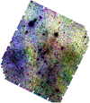 |
Fig. 1. RGB image of the A 2390 galaxy cluster Euclid FoV. The contrast is greatly enhanced to highlight large-scale colour variations (due to cirrus and background inhomogeneities) across the whole image in the LSB regime. Blue is VIS, green is the JE band, and red is the YE band. North is up and east is to the left. |
Previous papers have studied the wavelength dependency of Galactic cirrus, showing that the dust-scattered component is prominent in optical bands with a decreasing albedo in the NIR (Román et al. 2020; Zhang et al. 2023). The trend is similar in A 2390 images, as more prominent cirrus features were observed in the VIS image compared to the NISP ones. The least affected band seems to be HE. In the case of A 2390, the cirrus presents colour variations across the FoV, especially comparing VIS to NISP (see Fig. 1), indicating a heterogeneous ISM with a spatially and spectrally varying composition, probably due to the varying column density of the dust clouds (e.g. Román et al. 2020).
3.2.1. FIR dust maps
At longer wavelengths, cirrus has its peak emission in the FIR due to thermal emission from low-temperature dust (Low et al. 1984; Veneziani et al. 2010) which roughly correlates with optical surface brightness (Witt et al. 2008). This led previous ICL studies to assume a spatial match between FIR dust maps and optical/NIR cirrus light (Mihos et al. 2017; Kluge et al. 2020). In particular, Kluge et al. (2025) corrected for significant cirrus contamination in Euclid's ERO VIS image of the Perseus cluster by empirically scaling the Planck/WISE 12-μ dust map.
A procedure similar to Kluge et al. (2025) was attempted to remove the foreground cirrus in the A 2390 images, using the dust emission maps from Meisner & Finkbeiner (2014). This map was generated from the WISE 12-μ imaging data and is free of compact sources and other contaminating artefacts. The angular resolution of these dust maps is 26″ per pixel. We tried different normalisations of this dust map to match the average background properties of the Euclid images. Unfortunately, none of the normalisations provides a reliable cirrus subtraction, leaving a significant amount of filamentary cirrus in the residuals, especially over the location of A 2390. An example is shown in Appendix A. In this case, the resolution of the dust maps does not describe the distribution of the cirrus. Since the cluster's size is similar to the size of the dust filaments, this method is not optimal.
The different spatial resolutions between the FIR maps and optical observations are the main source of this disparity. In addition, the FIR to optical/NIR similarity is a first-order approximation to the complex multi-phase Milky Way (MW) ISM, which may include different populations of dust grains (composition, size, and geometry) in a variety of physical conditions (local radiation field, density, and temperature), see Draine & Li (2007) and Brandt & Draine (2012).
Following these preliminary tests, we concentrated on the NISP images that are less contaminated by cirrus. As the cirrus covers the whole FoV, most of its distribution varies over angular scales much larger than the extent of A 2390. Therefore, an alternative empirical wavelet-based approach was chosen for direct cirrus modelling and removal in the NISP images (see next section).
3.2.2. Multiscale modelling
We performed a multiscale decomposition of the images to disentangle the large-scale cirrus signal (covering most of the FoV) from the smaller angular scale (1 to a few arcminutes) extragalactic sources, ICL included. This part of the analysis was based primarily on the Detection Algorithm with Wavelets for Intracluster light studies (DAWIS; Ellien et al. 2021). The detailed operating process of DAWIS is described extensively in Ellien et al. (2021), so only salient points are summarised here. DAWIS leverages a wavelet representation (Slezak et al. 1994) and multi-resolution vision models (Bijaoui & Rué 1995) to separate small-scale details from large-scale variations in the analysed images. For this purpose, an isotropic undecimated wavelet transform (Starck et al. 2007) is applied to the image, decomposing it into N wavelet planes of the same size. The noise is estimated and modelled in the first wavelet scale before being extrapolated to larger scales to detect sources by thresholding these maps. These regions of significant wavelet coefficients are linked into interscale trees, which are then used to reconstruct the corresponding 2D light distribution in the original image. The distinctive feature of DAWIS is its iterative strategy: it models only a few sources at a time (controlled by a threshold factor τ)2 starting with the brightest and removing a fraction of their 2D light profile (controlled by a mitigation parameter γ)3 from the image. The whole process (from the wavelet transform to light profile modelling) is repeated until it converges on a residual map that contains only noise. At each iteration, the detected and modelled sources correspond to substructures rather than entire astrophysical objects. These are termed ‘atoms’; since the sum of all these light contributions reproduces a fully noise-free version of the astrophysical field. One can also select a fraction of the atoms based on criteria (size, morphology, wavelet scale…), and sum their light profiles to synthesise and model specific astrophysical sources.
For this work, DAWIS was complemented by a mixture of gnuastro (Akhlaghi & Ichikawa 2015) and photutils (Bradley et al. 2024) routines. First, the NISP images were pre-processed to be suitable for a wavelet analysis: the astwarp routine was used to rotate the images (Θ = 65°) so the two axes of the image correspond to the two axes of the wavelet transform. The images were then cropped with astcrop to a box of size  covering all but a small fraction of the FoV. To reduce the computing time of DAWIS, the cropped images were binned by a factor of 4, resulting in images of size 2251 pix×2251 pix with pixel scale
  . As the goal is to model and remove the large-scale cirrus background, the loss of some small-scale information inserted into the analysis by these operations is not an issue. Moving forward, DAWIS was run on the resulting images with input parameters set to ensure a quick but rough-quality reconstruction of small and compact sources. This ensured that the algorithm quickly reached the larger wavelet scales. Therefore, following values advocated by Ellien et al. (2021), τ and γ were set to 0.1 and 1, respectively.
The two assumptions made to select the cirrus distribution atoms were: (i) its distribution varies over larger angular scales than the ICL, so its information is encoded in atoms detected at lower-frequency wavelet scales, (ii) its distribution should not feature a peak centred on A 2390 position on the sky, as this would rather be ICL. After visual inspection of the outputs, the cirrus maps were derived by selecting atoms detected at wavelet scales ≥6, ensuring that we only keep sources larger than a few arcminutes. Note here that some bright foreground MW stars that were not PSF-subtracted in the images are larger than this characteristic size, so part of their atoms were also selected and included in the cirrus maps. This is not a problem in this analysis because these stars are located far from the full extent of A 2390. To minimise removal of ICL from A 2390, a hand-made ellipse ( with a 30° angle and centred on
  ,
,  ) was made to roughly cover the cluster extent. All atoms with peak coordinates of their light distributions within the ellipse were not included in the cirrus map. Additional attention is brought to the DAWIS residuals, and a large-scale gradient was still noticeable after the whole wavelet procedure. Since the cirrus signal occupies most of the FoV, it is difficult to distinguish it from the true sky background, so the two were combined into a cirrus + background map. To do so, the residuals were fitted with the Background2D function from photutils, with a box size of 40 pix×40 pix and a median filter of size 3 pix×3 pix, and the resulting 2D background was added to the cirrus map. The cirrus maps were then scaled back to the original NISP pixel scale and orientation. The cirrus-corrected images were then produced by subtracting these from the original image, as shown in Fig. 2. A first-order estimation of the surface brightness cirrus model was made by using as sky background the mean value of the noise in a vertical strip of width
  on the right edge of the original images (which show less cirrus contamination, see Fig. 2). This gives median surface brightness values for the cirrus model of 26.3, 26.1, and 26.1 mag arcsec−2, with maximum peaks of 23.9, 24.2, and 23.9 mag arcsec−2 for the brightest filaments in the YE, JE, and HE bands respectively4. The surface brightness limits (3σ, 10 ″×10 ″) of the cirrus-subtracted NISP images are 29.3, 29.4, and 29.4 mag arcsec−2 for the YE, JE, and HE bands, respectively, which is about 0.4 mag deeper than the original images.
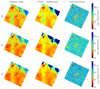 |
Fig. 2. Effect of cirrus removal for all NISP filter images. Left to right: Original image; cirrus+background map; cirrus-corrected image. The angular size of the images is |

3.2.3. Limitations and uncertainties
An intrinsic issue of the empirical process described in the previous section is the inability of an artificial wavelet scale separation to capture all subtleties of the hierarchical cirrus light distribution. While most of the large-scale cirrus is captured and modelled, some of the finer filaments (e.g. of similar size as extragalactic sources) are visible in the cirrus-corrected images (especially in the YE band, see Fig. 3). This inevitably leads to some flux-positive cirrus contamination left in the corrected images that might locally increase the ICL light level and bias colour measurements. For similar reasons, another effect occurs as some of the larger-scale ICL can be accidentally included in the cirrus map and removed from the image. To estimate the uncertainties resulting from these effects and their influence on the ICL, a series of tests was performed, based on mock clusters inserted in the HE image.
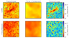 |
Fig. 3. Zoom-in on regions of interest in the YE band, which displays the most cirrus residuals after correction. Top row shows a |


The process of creating the mock clusters and their ICL is similar to the one described in depth in Euclid Collaboration: Bellhouse et al. (2025), so we only provide a quick summary here. The most massive cluster from the MAMBO simulated light-cone catalogue (Girelli 2021) was used for the mocks. The ICL, BCG, and satellite galaxy images were produced using the galsim (Rowe et al. 2015) package. Satellite galaxies were modelled with Sérsic profiles having either single-component or two-component bulge+disk profiles, whilst the BCG and ICL were generated as Sérsic components using the mean values of double-Sérsic decompositions performed by Kluge et al. (2020), scaled to the stellar mass of the cluster. All light profiles were convolved with the Euclid PSF. The same cluster was inserted with the same orientation at nine different positions within the Euclid observation, chosen to cover a varied range of cirrus intensities to measure the effect of subtracting different levels of cirrus on the resulting flux of the ICL.
The same cirrus modelling process as in Sect. 3.2.2 was applied to the image with the mock clusters. BCG+ICL radial intensity profiles were derived in circular apertures for all mocks, before and after the cirrus correction. Figure 4 shows the BCG+ICL profiles before (red) and after (blue) cirrus correction, alongside the true BCG+ICL profile used for the mock clusters and the difference between them. The effect of the cirrus on the profiles is the strongest in the outer part (>100 kpc), as the profiles before cirrus correction display significant disparity depending on local cirrus properties and large deviations from the true values (reaching values larger than 2 orders of magnitude for most of the clusters). After cirrus correction, this disparity is greatly reduced, reducing the deviation from the true profile to absolute values below 0.5 orders of magnitude for most clusters, out to 600 kpc and down to surface brightness values of 30 (see lower panel of Fig. 4).
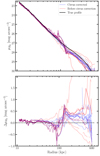 |
Fig. 4. Top: Mock cluster radial profiles in the HE band before (red) and after (blue) cirrus correction. The true BCG+ICL light profile is shown as a black line. Bottom: Difference between the true BCG+ICL light profile and the measured BCG+ICL profiles. |
3.3. Selection of cluster member galaxies
We extracted a catalogue of all galaxies with redshifts available within a radial aperture of 30’ around A 2390 from the NASA Extragalactic Database (NED)5. There are 488 galaxies with spectroscopic redshifts. The redshift histogram peaks at the cluster redshift, and is quite clearly limited to the [0.2169, 0.2369] interval, which we consider hereafter as the cluster range. There are 184 galaxies with redshifts in this interval. The corresponding velocity range is [58 147, 62 839] km s−1.
In addition to the spectroscopic members, we supplemented our membership (particularly in the core of A 2390) using the high-probability members (Pmem>0.8) from the SDSS-redMaPPer (Rykoff et al. 2014) catalogue. We note that redMaPPer only uses galaxies with SDSS i<21.0 and that the red-sequence-based cluster redshifts provided by redMaPPer are consistent with existing spectroscopic redshifts (Rykoff et al. 2014). 28 of these redMaPPer galaxies are spectroscopic members (matched members within a  radial distance of our spectroscopic member catalogue described above) and the SDSS photometry provide us with more accurate galaxy positions. After visual inspection of each source, this resulted in a catalogue of 219 galaxies that can be considered as belonging to the cluster. A
  cutout of A2390 with these galaxies highlighted is shown in Fig. 5. This catalogue was used to compute a galaxy density map of cluster members (see Sect. 5.4.1), as well as galaxy morphology distributions (see Sect. 5.4.2).
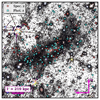 |
Fig. 5. Image of the |

The cluster member catalogue was then cross-matched with the ERO object catalogue (Cuillandre et al. 2025), which contains photometric information for the four Euclid bands of the whole FoV, obtained by running SEXTRACTOR (Bertin & Arnouts 1996) on both the VIS and NISP data. The MW extinction corrections for each Euclid filter were derived using the Planck thermal dust map (Planck Collaboration XI 2014; Gordon et al. 2023) extinction law, assuming a 5700 K blackbody spectral energy distribution.
3.4. Masks
To accurately measure the properties of the diffuse light of A 2390, all sources except the BCG and ICL must be masked. We used the PSF-cirrus-subtracted NISP images in the separate YE, JE, and HE bands from Sect. 3.2.2 to start the masking process. Next, the masks were combined to obtain a final NISP mask (YE+JE+HE). Additionally, while subtracting the stellar PSF model effectively removes the diffuse extended wings of the PSF (Sect. 3.1), the central regions show significant residuals. Therefore, the bright star central regions were masked with a circular patch of 70 pixels (210 ″) in radius.
As these are deep images, the masking must be optimised for faint and compact background objects as well as those that are larger. To do so, we used SEXTRACTOR in a ‘hot+cold’ masking mode, similar to the method used in Montes & Trujillo (2014, 2018) and Montes et al. (2021). The ‘hot’ mode is optimised to detect the small and faint sources and was run using the following steps:
-
(i)
The contrast of the image is enhanced by creating an unsharp-masked version in each band.
-
(ii)
The unsharp-masked image is made by convolving the original image with a box filter with a side of 15 pixels (45 ″) and then subtracting the convolved image from the original.
-
(iii)
SEXTRACTOR is run on the unsharp-masked image with the source detection threshold of 1σ above the background.
The ‘cold’ mode is used to find large and diffuse sources, which was achieved by running SEXTRACTOR with a minimum source size of 40 pixels and a 5σ detection threshold. Finally, the hot and cold modes were combined along with the circular bright star masks to create three different masks: (i) a mask for all sources; (ii) a mask for all sources except the BCG+ICL, and (iii) a mask for all sources but the BCG+ICL and cluster members (see Sect. 3.3 for details).
Each mask required some additional steps. The mask for all sources was created to measure any potential residual background light in the image (see Sect. 4.3.1). Therefore, it is essential to mask the ICL along with the galaxies for this step. To achieve this, the cold masks were radially extended by 15 kpc (4 ″) and the hot masks were radially extended by 5 kpc ( ) at the cluster redshift. These extensions were chosen after visual inspection. Finally, a 3σ clipping was applied around the mean value of the remaining pixels to mask any residual high/low-value pixels not detected by SEXTRACTOR during the masking process above. This last sigma clipping step was not done in masks (ii) and (iii) because this process also masks some pixels from the extended BCG light. Masks (ii) and (iii) were also prepared for a 2 Mpc×2 Mpc cutout around the cluster centre, while mask (i) was made for the entire A 2390 Euclid FoV.
4. Measuring the ICL of A 2390
Although the qualitative definition of ICL as light emitted by stars not bound to the galaxy, distributed throughout the cluster's gravitational potential, is straightforward, its photometric observational signature is ambiguous, especially regarding its strong and smooth entanglement with the BCG light profile. This lack of consensus stacks on top of other generic LSB astronomy challenges (such as cirrus contamination; see Sect. 3.2) making the detection and characterisation of ICL challenging. As a result, many ICL measurement strategies have been developed by observers, often independently from one another. This lack of a definition inevitably leads to disparities when comparing results, such as ICL and BCG+ICL fractions. Recently, Brough et al. (2024) addressed this issue by testing several observational methods on state-of-the-art simulations, finding that the different methods are consistent.
Inspired by the robust multiplex analysis presented in Brough et al. (2024), three of the methods used in that analysis were used here to detect, characterise, and model the ICL: 2D multi-galaxy fitting (CICLE, Jiménez-Teja & Dupke 2016); wavelet-based multiscale analysis (DAWIS, Ellien et al. 2021); and mask-based 1D profile fitting (Ahad et al. 2023). These methods are described in more detail in the following sub-sections.
4.1. CICLE
The CHEFs Intracluster Light Estimator (CICLE, Jiménez-Teja & Dupke 2016) is a multi-galaxy fitting algorithm, that isolates the ICL by modelling and subtracting the light from galaxies. CICLE fits galaxies using mathematical bases composed of Chebyshev rational functions and Fourier series (CHEFs, Jiménez-Teja & Benítez 2012), which are very flexible and capable of modelling galaxies with any morphology. However, objects with sharp features, such as saturated stars, diffraction spikes, or objects cut in the borders of an image, lie outside the space of elements that can be fitted by CHEFs. Although we generated PSF-subtracted images (see Sect. 3.1), they still contain diffraction spikes that CHEFs cannot fit (Fig. 5). For this reason, we first masked all the stars located within the A 2390 field, then later ran SEXTRACTOR to detect the galaxies and, finally, model and remove them with CICLE.
The modelling of the BCG represents a challenge for any galaxy method, given its spatial coincidence, in projection, with the ICL. Indeed, the BCG is usually surrounded by a diffuse and extended halo that is complex to disentangle from the ICL. To outline the boundaries of the BCG-dominated region, CICLE calculates a curvature map, which expresses for each point of a surface, the local change in the slope of the surface at that point with respect to the surroundings. When the surface is the projected distribution of the composite BCG+ICL system, we can separate the two components because they usually have different slopes. CICLE naturally traces the transition from the BCG- to the ICL-projected distributions (or more specifically, where each one of the two distributions dominates) by identifying the curve of points where the curvature changes most.
CICLE operates in two dimensions, so no intrinsic assumptions on the shape or symmetry of the sources were made (either for the galaxies or the ICL). CICLE has been tested against simulations (Jiménez-Teja & Dupke 2016), which find that it has an error of less than 1% in ICL measurements made on clusters between 0.2<z<0.3, the redshift range that includes A 2390. For A 2390, we ran CICLE on the cirrus- and background-removed images derived in Sect. 3.2.2 with a standard configuration. This gave each band an image containing only ICL and noise, in which the measurements in the following sections were made. A BCG+ICL map was also produced by re-inserting the BCG model into the image (see Fig. 6), and a total cluster map was created by re-inserting the models of all galaxy members.
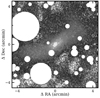 |
Fig. 6.
|

4.2. DAWIS
A BCG+ICL map was produced using DAWIS, already introduced in Sect. 3.2.2. The process was similar to what was described for the cirrus modelling, although adapted to ICL detection. The cirrus-corrected image of each NISP band was cropped to a box of size  centred on the BCG, resulting in images of size 3600 pixels × 3600 pixels. DAWIS was run on these images with input parameters enabling refined source modelling, with τ = 0.1, γ = 0.5, and a maximum number of wavelet planes of 9. Most of the ICL was modelled by selecting and summing the light profiles of atoms detected at wavelet scales greater than 5 (as advocated by Ellien et al. 2021; Ellien 2025) and with maximum peak coordinates inside an ellipse covering the extent of the cluster. Atoms detected at lower wavelet scales, and with maximum peak coordinates inside 5 ″ radius around the BCG centre were also kept to model the smaller BCG core profile. The two were summed to produce for each filter the BCG+ICL model used in the rest of the analysis (the JE band is displayed as an example in Fig. 7). Finally, the masks produced in Sect. 4.3 were used as priors to select atoms belonging to satellite galaxies: atoms with maximum peak coordinates within any galaxy mask were kept, and their light profiles were summed to produce a satellite galaxy map. A total cluster map was also produced by summing the BCG+ICL and the galaxy maps.
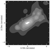 |
Fig. 7.
|

4.3. 1D profiles
The third method to measure the ICL is the mask-based 1D profile fitting (hereafter ‘Ahad’, Ahad et al. 2023), which can be used to measure the 1D BCG+ICL profile of A 2390. The advantage of deriving the profiles in a non-parametric way is that it makes no assumptions regarding the shape of the system. Therefore, we do not assume any particular model to describe the BCG+ICL, since the results might be sensitive to the choice of the particular model and prone to degeneracies between the different parameters.
4.3.1. Residual background profiles
Although we measured the surface brightness profiles from the PSF-cirrus-background-subtracted NISP images, there can be a low-level residual background (leftover cirrus, instrumental scattering, or zodiacal light), which can bias the ICL measurements and is likely to have an irregular distribution throughout the image. Therefore, we measured the SB profile of the residual background in 30 random locations throughout the A 2390 FoV. The background SB profiles were measured in a similar way to that of the BCG+ICL profile (see Sect. 4.3.2), centred at each random location, using the mask for all sources from Sect. 3.4. The random locations were generated between 2000 and 10 000 pixels along both x and y directions to ensure that at least half of the random cutouts are always in the image. If any of the 2 Mpc×2 Mpc cutouts of the 30 random background profiles had more than 50 per cent pixels masked, it was removed from the stack. Finally, the average background profile was measured.
Figure 8 shows the distribution of the residual background pixels for the three NISP bands. As expected from the already background-removed images, their median values are within 1σ of 0, as shown in the histogram (with median values of background pixels indicated with vertical lines in the same colours as the histograms according to the NISP filters). We note the YE band displays a mean value slightly higher than 0, probably due to higher cirrus residuals for this filter (see Sect. 3.2.3). This is also highlighted in Fig. 9, where the maximum difference in the flux density profile of the BCG+ICL before (top panel) and after (bottom panel) the residual background removal is in the YE band.
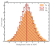 |
Fig. 8. Histogram of background pixels in the three cirrus-subtracted NISP bands. Because the background was also removed during the process, all three distributions are centred close to zero. |
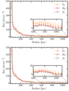 |
Fig. 9. Surface brightness profiles of the BCG+ICL in the three NISP bands before (top panel) and after (bottom panel) subtracting the residual background. The flux density values are shown with a magnitude zero-point of 30. |
4.3.2. Measuring surface brightness profiles
The 1D azimuthally averaged profiles were created using circular apertures centred at the BCG of A 2390 out to 1 Mpc radial distance. The central parts of the profiles were linearly binned from one to 10 pixels for better sampling; logarithmic binning was used beyond that. Masks (ii) and (iii) from Sect. 3.4 were used to calculate the BCG+ICL and total cluster light profiles from the unmasked pixels, respectively. The average residual background profiles (Sect. 4.3.1) were subtracted from the BCG+ICL and total cluster light profiles. Finally, the surface brightness radial profiles, shown in Fig. 10, were converted to mag arcsec−2.
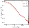 |
Fig. 10. Surface brightness radial profiles for the BCG+ICL of A 2390 from the 1D method Ahad. Profiles for the YE (orange), JE (red), and YE (dark red) NISP bands are shown. |
5. Results
5.1. Surface brightness radial profiles of BCG+ICL
We derived the radial profiles in each of the three NISP bands following a similar methodology as in Ahad et al. (2023), as described in Sect. 4.3.2. The 1D radial surface brightness profiles as a function of radius for the YE (orange), JE (red), and HE (dark red) bands are shown in Fig. 10.
We conservatively decided not to explore the ICL beyond 600 kpc, since the uncertainties become too large (>0.5 mag arcsec−2). The BCG+ICL profile roughly follows a Sérsic (1968) profile, out to 50 kpc where we start seeing more structure in the profiles. This is probably due to some unmasked light from satellite galaxies, which is already too dispersed and mixed into the ICL for us to mask it properly. Around 70–80 kpc, we see an excess in the profile's extension in the inner 50 kpc, a signature of accreted material, i.e. the ICL. Such radius is consistent with BCG-to-ICL transition radii from both observations and simulations (60±40 kpc; Zibetti et al. 2005; Gonzalez et al. 2005; Iodice et al. 2016; Zhang et al. 2019; Contini et al. 2022; Brough et al. 2024).
5.2. ICL fractions
Measuring the amount of light in the ICL with respect to the total light of the cluster (brightest cluster galaxy, satellite galaxies, and ICL), the ICL fraction enables us to evaluate the efficiency of the processes that shaped the cluster. Exploring the BCG+ICL fraction (the amount of light in the BCG+ICL with respect to the total light of the cluster) can give us clues about their common evolution.
Table 1 shows the BCG+ICL and ICL fractions (and luminosities) of A 2390 derived with the three methods presented in this work, namely, CICLE, DAWIS, and the 1D profile Ahad method. The ICL and BCG+ICL fractions were derived independently in each method, using their respective ICL, BCG+ICL, and total cluster light integrated flux values. For consistency, all integrated flux values were computed within 600 kpc from the BCG centre.
ICL and BCG+ICL fractions and luminosities of A 2390, measured by the different methods explored in this work, namely CICLE, DAWIS, and 1D Profile Ahad.
All methods used the same way to separate the BCG from the ICL: cutting out the inner 50 kpc of the BCG, as in Euclid Collaboration: Bellhouse et al. (2025), to produce results compatible with future Euclid ICL studies. For the Ahad method, the BCG+ICL and total cluster (BCG+ICL+satellites) fluxes were computed by integrating their respective profiles, out to 600 kpc. To measure the ICL flux, we integrated the BCG+ICL 1D profile from 50 to 600 kpc. For the CICLE and DAWIS methods, the BCG+ICL fluxes were computed by integrating the respective BCG+ICL maps, out to 600 kpc. The ICL flux was computed by integrating the BCG+ICL maps from 50 to 600 kpc. In the same way, the total cluster flux was derived from their respective total cluster maps (as described in Sect. 4.1 for CICLE and Sect. 4.2 for DAWIS), integrating out to 600 kpc.
Although a detailed comparison between the methods is beyond the scope of this paper (for more information on this see Brough et al. 2024), we see that the fractions derived are roughly similar. The average BCG+ICL fraction is 29%, for all bands and all methods, and the average ICL fraction is 24%. Note that the CICLE fractions appear slightly higher than DAWIS and Ahad. However, this difference is only a few per cent, and is compatible within uncertainties.
The BCG+ICL fractions quoted here (29% for all bands and methods) are in agreement with those in the literature for clusters at the redshift of A 2390 (z∼0.23, Zhang et al. 2019; Furnell et al. 2021; Sampaio-Santos et al. 2021). It also agrees with the fractions from Gonzalez et al. (2005), Kluge et al. (2021), and Ragusa et al. (2023) of nearby massive clusters. The ICL fraction is on average 24%, which agrees with the estimates of Burke et al. (2015), Furnell et al. (2021), Zhang et al. (2024), and Golden-Marx et al. (2025) although it is towards the higher end. This could be because A 2390 is a very massive cluster (M200, c = 1.6×10¹⁵ M⊙). The small difference between the ICL and BCG+ICL fraction (24% versus 29%), suggests that most of the light in the BCG+ICL in this cluster is in the ICL. The fraction of the ICL over the BCG+ICL component is on average ∼80%, which is high compared to the values for other clusters (typically around 65–70%, see Figure 5 in Montes 2022). This higher fraction is remarkable considering we do not include the ICL light in projection to the BCG in the inner 50 kpc, making it a lower limit. On the contrary, note that increasing the 50 kpc separation cut to larger radii would diminish the ICL fraction.
5.3. Colours of the ICL and satellite galaxies
Radial colour gradients constrain the physical processes that build up the ICL, and consequently, the BCG (Zibetti et al. 2005; Montes et al. 2014, 2021; DeMaio et al. 2015; Spavone et al. 2020; Ragusa et al. 2021, 2022; Golden-Marx et al. 2023). Each process, such as tidal stripping or galaxy mergers, leaves a distinct imprint on the stellar population reflected in its spectra and the measured colours. For this reason, comparing the colour of the ICL with that of the satellites reveals clues about its progenitor population (see Montes 2019; Arnaboldi & Gerhard 2022; Contini et al. 2024b, and references therein for in-depth discussions on this subject).
Figure 11 shows the radial YE−HE colour profile of the BCG+ICL of A 2390. We use this colour to study the stellar populations of the BCG+ICL system because it covers a wider wavelength range than any of the other colours. In Fig. D.1 in Appendix D, we show the Euclid NIR colour from the Vazdekis et al. (2016) stellar population models.
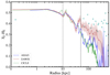 |
Fig. 11. Colour radial profiles for the BCG+ICL system of A 2390. Green diamonds represent the cluster selected members, while red, blue, and green lines are the ICL radial profiles estimated with the three methods presented in Sect. 4: Ahad in blue; CICLE in green; and DAWIS in red. The vertical lines indicate 10 and 50 kpc, to guide the eye. |
We derived colour profiles for the three methods described in Sect. 4. For the 1D profile method, we subtracted the profiles derived in Sect. 4.3. The radial surface brightness profiles, and therefore colour profiles, for DAWIS and CICLE were derived in a similar way as in the Ahad 1D profile method: using circular annular apertures on the 2-D BCG+ICL maps that result from the two methods described in Sect. 4. We used small steps in radial distance to better trace the ICL's behaviour.
In Fig. 11, we overlay the colours for the cluster members (light green diamonds), which are computed using the photometric values from the member catalogue presented in Sect. 3.3. The MW extinction corrections for each Euclid filter were derived using the Planck thermal dust map (Planck Collaboration XI 2014; Gordon et al. 2023) extinction law, and assuming a spectral energy distribution of a 5700 K blackbody (following the same method as described in Kluge et al. 2025).
The cluster members do not show any radial dependence in their colour from the core to the outskirts (though we note that this is probably linked to the cluster member selection method). The BCG and cluster members have a mean colour of YE−HE = 0.39. Cluster member colour histograms are shown in Appendix C. The colour profiles of the BCG+ICL present two distinct regions: flat in the core out to 5 kpc; and a negative slope from 5 to around 450 kpc. The flat colour profile at <5 kpc is consistent with a mixing of the stellar populations in the centre of the BCG, while the negative colour gradient at >5 kpc indicates a gradient in the stellar populations of the BCG+ICL system: they become bluer with radius. Because the YE−HE colour mainly traces a change in metallicity (Appendix D), this indicates that the stellar populations become metal-poor with radius due to the accretion of smaller systems into the BCG. We also note that because of modelling uncertainties, the DAWIS colour profile is redder at large radii (>200 kpc) than seen in the other two methods.
5.4. The spatial distributions of A 2390 cluster members
As discussed, colour gradients indicate that the ICL is at least partially formed through tidal stripping of satellite galaxies. While some of this occurs when satellites fall into the cluster, tidal stripping also occurs when satellite galaxies interact with the BCG. Therefore, comparing the spatial distribution of the ICL to that of the satellites may inform our understanding of the population of galaxies that form the ICL.
5.4.1. Galaxy density map
To investigate this, we first look at the spatial distribution of the entire sample of 219 potential cluster members described in Sect. 3.3 by measuring a density map, as shown in Fig. 12. For this density map, we used the adaptive kernel technique with a generalised Epanechnikov kernel (Silverman 1986). This implementation is summarised in Dantas et al. (1997), based on an earlier version developed by Timothy Beers (ADAPT2) and improved by Biviano et al. (1996). The statistical significance is established by bootstrap resampling of the data. We performed 100 bootstrap realisations with a pixel size of  and the density map was computed for each realisation. For each pixel of the final bootstrap map, the value was taken as the mean over all realisations (see Durret et al. 2016).
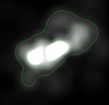 |
Fig. 12. Density map of the 219 galaxies selected as belonging to the cluster A 2390 (see main text). The green contour levels correspond to 3σ, 10σ, and 20σ above the background. North is up and east is to the left. The image size is |

We derived the significance level of our detection by estimating the mean value and dispersion of the background. For this, we drew histograms of the pixel intensities and fit them with a Gaussian, as illustrated in Durret et al. (2016). The mean value of the Gaussian gives the mean background level, and the width of the Gaussian is the dispersion, σ. We then computed the contour values corresponding to nσ detections as the background plus nσ.
In Fig. 12, we see an elongated distribution of the satellites with a similar shape and ellipticity to what is seen for the ICL in Fig. 7. Interestingly, we appear to see two distinct populations, the main cluster and a smaller secondary population in the south-east. This distribution does not change if we only include the spectroscopic members.
5.4.2. Galaxy morphology distribution
While Fig. 12 suggests a similar spatial distribution between the ICL and the satellites, it does not tell us whether all satellite galaxies trace the ICL. Each cluster member's morphology (using the sample described in Sect. 3.3) was visually classified by two of the authors (JBGM, PD) as either elliptical or spiral using the Euclid VIS images. Although some member galaxies have previous morphological classifications (Abraham et al. 1996), Euclid's higher resolution improved the accuracy of these classifications.
For the analysis shown in Fig. 13, we focussed on the 129 members of A 2390 within a projected distance of 1 Mpc of the BCG (corresponding roughly to half the virial radius; Li et al. 2009) and divided our sample into spirals (shown in blue) and ellipticals (shown in red). Although these cluster members all lie upon a tight red sequence (see Fig. C.2), not all are morphologically elliptical; a number have spiral features only visible due to Euclid's high spatial resolution. For each population, we oversampled the data and measured the number of galaxies within  (ten times the spatial resolution of the NISP data used to measure the ICL) of every point separated by
  (4 times the spatial resolution of NISP). We then constructed contours to identify the spatial distribution of the spiral and elliptical populations.
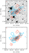 |
Fig. 13. Contour maps of the spatial distribution of elliptical (red) and spiral (blue) galaxies overlaid on the HE-band image of A 2390 in the upper panel, and the DAWIS BCG+ICL map in the lower panel. The figure shows a region of 700″×700″ (2.5 Mpc×2.5 Mpc) centred on the BCG. |
In Fig. 13, we show the contours of the spirals (in blue) and ellipticals (in red) onto the HE-band image of A 2390 in the upper panel and the DAWIS BCG+ICL map in the lower image. These contours allow us to directly compare how the distribution of morphological populations of satellite galaxies align with the cluster (upper panel) and BCG+ICL (lower panel). In agreement with Abraham et al. (1996) and our understanding of red sequence formation (e.g. Gladders & Yee 2000; Rykoff et al. 2014), these contours show that the central region of the cluster is predominantly populated by elliptical (red) galaxies. Moreover, the comparison between the satellite galaxy distributions and the DAWIS BCG+ICL model in Fig. 13 illustrates that the elliptical galaxies (red) cause the alignment between the ICL and satellite population. The spiral spatial distribution (blue), on the other hand, is more scattered and is shifted towards the south-west – it does not trace the entire ICL but rather substructures. We note that the satellite galaxy and ICL distributions identify similar features, most noticeably the asymmetry in the north-west direction. The elliptical satellite contours, similar to Fig. 12, identify a secondary population of galaxies in the south-east direction. This subgroup appears to have more spiral galaxies than the core. However, the most significant observation is that the contours of the elliptical galaxies suggest that the galaxy distribution centroid is offset from the BCG by about 20″ (≈ 70 kpc).
5.4.3. Detection of substructures
We applied the DS+ algorithm (Benavides et al. 2023) to detect groups among the 184 cluster members spectroscopically identified in Sect. 3.3. DS+ is an updated version of the Dressler & Shectman (1988) algorithm, which compares the local velocity field around each galaxy with that of the whole cluster. Statistically significant departures of the two distributions are indicative of the presence of a group. DS+ also identifies the galaxies that compose the groups with a statistical approach. Under the ‘non-overlapping’ mode, this identification is unique, meaning each galaxy is assigned to a single group and cannot belong to several groups simultaneously.
We set DS+ with a probability threshold of 0.1 and ran it with 1000 simulations in the non-overlapping mode, as recommended in Benavides et al. (2023). We identified six groups with more than four members; their positions are shown in Fig. 14 and their properties are described in Table 2. Note that groups 1, 2 and 4 fall outside the field of view shown in Fig. 14.
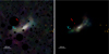 |
Fig. 14. RGB images of the BCG+ICL in the core of A 2390 (700 ″×700 ″). The left panel shows the CICLE RGB map and the right panel the DAWIS RGB map. The numbers in both maps mark the position of the galaxies in the groups identified by DS+ (see Sect. 5.4.3), listed in Table 2. Both colour images were generated with Trilogy (Coe et al. 2012). |
Properties of the six groups identified by the DS+ method: group identifier, number of members, distance to the centre of the cluster, velocity dispersion, and mean velocity.
Figure 14 shows RGB maps from CICLE (left) and DAWIS (right) created from the BCG+ICL maps for each of the NISP bands. As shown in Fig. 14, the different groups follow the overall ICL distribution. In particular, groups 5 and 6 are associated with the south-eastern ICL structure, whereas group 3 may be infalling from the west6.
The colours of the ICL patches in Fig. 14 are not homogeneous, a sign that the ICL in these groups is not well-mixed yet. For example, the ICL in the north-western direction appears bluer, while the ICL associated with group 5 shows an intermediate colour (green). Nevertheless, these patches have a similar characteristic size as some of the cirrus filament residuals seen in other areas of the cirrus-corrected images (see Sect. 3.2.3 and Fig. 3). We do not rule out that these colours might be affected by cirrus contamination.
5.5. Comparison with total mass and X-ray maps
One of the primary goals of Euclid is to map the mass distribution in the Universe using weak gravitational lensing measurements. The ICL is an effective tracer of dark matter in clusters (Montes & Trujillo 2019; Alonso Asensio et al. 2020; Sampaio-Santos et al. 2021; Yoo et al. 2024). Therefore, the ICL provides an additional constraint to improve these derived mass distributions in clusters. In addition, the comparison of ICL, X-ray, and mass map distributions can give us clues about the dynamical state of the cluster (e.g. Kluge et al. 2025).
Here, we compare the 2D distribution of dark matter in A 2390 (as traced by gravitational lensing models) with the X-ray and BCG+ICL (DAWIS HE) maps. For this, we followed the steps outlined in Montes & Trujillo (2019), summarised below.
We used the mass map of A 2390 as derived in Diego et al. (in prep.). The map is a joint strong+weak lensing solution using WSLAP+ (Diego et al. 2005; Sendra et al. 2014). WSLAP+ is a free-form code, that is, it does not assume any mass distribution. It improves the Atek et al. (2025) results by adding new photometric redshift estimates for the galaxies in the Euclid FoV. To compare the shape of the cluster X-ray emission to the mass and ICL distributions, we also retrieved Advanced CCD Imaging Spectrometer (ACIS) images of A 2390 from the Chandra Data Archive7. The X-ray maps are from Observation 4193 (PI: S. Allen).
We derived the isocontours for the three components: BCG+ICL; total mass; and X-rays. For a sensible comparison, the isocontours of each map were obtained at the same physical radial distances: 50, 100, 150, 200, 300, 500, 600, and 700 kpc. To do that, we derived radial profiles of the three components. Note that the purpose of these radial profiles is to obtain an intensity at a given radial location to derive the isocontours for each of the three components.
We assumed the centre for each of the maps to be the location of the BCG, since the peaks of the mass map and the X-rays are also located there. Then, we obtained the radial profiles of the BCG+ICL, X-ray emission, and mass. The profiles were constructed by averaging over circular bins out to 1 Mpc. Once the intensities at the different radial distances were obtained, we used contour in matplotlib to obtain the isocontour lines. Figure 15 shows the comparison between the contours (shapes) of the different components. The black and white background is the DAWIS BCG+ICL map, while the contour lines show the X-rays (orange) and the mass (blue) distributions.
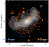 |
Fig. 15. Region of 700″×700″ around A 2390. The background is the ICL filled-contour map from DAWIS (HE band) while the blue and orange lines are the mass and X-ray contours, respectively. The contours are at 50 (lightest shade), 100, 150, 200, 300, 500, 600, 700 kpc (darkest shade). |
At the very centre of the cluster, within 300 kpc, the three components are very similar to each other. Beyond 300 kpc, however, the three components begin to diverge. The X-ray contours show an asymmetry towards the south-east at about 300 kpc, although they become more regular again at larger distances. The BCG+ICL map appears more elongated (elliptical) than the mass and X-ray maps. The mass map is elongated along the north-east to south-east axis, as in the BCG+ICL map. Interestingly, towards the south-east the mass contours widen perpendicular to the axis, probably indicating the presence of the south-east group of galaxies. The same happens, although to a lesser extent, to the north-east. At larger radii, the contours are rounder than the diffuse light, more similar to the X-rays. Therefore, it appears that the mass map does not yet fully capture the true distribution of mass of the cluster at large radii.
6. Discussion
The results presented in this work show the extraordinary potential of Euclid to understand ICL formation. Below, we discuss the implications of our findings.
6.1. Formation process of the ICL of A 2390
The ICL records most of the relevant events happening during the cluster's formation. Studying the stellar properties of the ICL provides information on the timing of the formation and insights into the processes that drove the build-up of the ICL and of the cluster itself. Comparing the ICL properties with those of the cluster members provides clues about the progenitors of this light (Arnaboldi & Gerhard 2022; Contini et al. 2024b).
Section 5.4.2 shows that the population of elliptical galaxies dominates the cluster's core, and follows the distribution of the ICL very well. This similarity suggests that these two components are linked and may have a common origin. The analysis of substructures reveals the presence of two main galaxy groups besides the central core of the cluster. Indeed, we detect ICL in the north-western ICL sub-halo, overlapping with a small group of red galaxies, and also within the south-eastern group. These are all signs that the ICL of A 2390 has an important contribution from the diffuse light of these smaller groups, the so-called pre-processing. This will be discussed in more detail in Sect. 6.4.
Radial colour gradients also provide relevant information about the physical processes that have formed or are forming the ICL and, consequently, the BCG. In Fig. 11, we present the YE−HE radial colour profiles of BCG+ICL for the three methods used in this work, namely CICLE, DAWIS, and the 1D profile method (Ahad). The colour profile shows a flat behaviour in the inner 5 kpc turning into a negative slope until around 450 kpc, becoming bluer with radius.
The central flatness suggests that the stellar populations of the inner 5 kpc are well mixed. This could be the case of a core (like Abell 85, Montes et al. 2021), a major merging event (e.g. Montes & Trujillo 2022) or caused by the presence of Hα emission (Alcorn et al. 2023). We discard the possibility that the cause of the flat colour is a core, since that would appear as a flat region of the same size in the surface brightness profiles in Fig. 10. However, the surface brightness profiles do not show this behaviour. Galaxies undergoing a major merger event could also produce a flat colour in the inner parts of the BCG+ICL profile (e.g. DeMaio et al. 2018; Montes & Trujillo 2022). The second brightest member of the cluster is located 120 kpc north-west from the BCG, and there is no massive galaxy in the very central region (r<10 kpc). There is also no evidence of plumes or other signs of interaction between these two galaxies in the Euclid images (see, for example, Martin et al. 2022). Alternatively, this flat colour could indicate a past major merger (see the cluster AS1063 in Montes & Trujillo 2018).
Hα emission has been detected in the BCG of A 2390 (Alcorn et al. 2023). This emission is produced by a cone, extending to the north-west direction of 15.9 kpc of length (but not aligned with the north-western subgroup). Alcorn et al. (2023) argue that star formation could be happening in this Hα cone, although more data are needed to support that. The IE image (the highest resolution) shows an elongation similar to that of the HST imaging (Alcorn et al. 2023). This emission is also seen in Spitzer (3.6 and 8 μm imaging), and probably causes a flat area at <5 kpc in the surface brightness radial profiles.
From 5 to approximately 50 kpc, we see a negative gradient in colour. Previous works reveal that the BCG+ICL profiles show negative colour gradients (Zibetti et al. 2005; Montes & Trujillo 2014; Mihos et al. 2017; Iodice et al. 2017; Montes et al. 2021; Golden-Marx et al. 2023; Zhang et al. 2024), indicating gradients in their stellar populations, generally metallicity (e.g. Peletier et al. 1990; Coccato et al. 2010; La Barbera et al. 2012; Huang et al. 2018; Santucci et al. 2020).
Figure D.1 shows the predicted colours of the Euclid NIR filters for the Vazdekis et al. (2016) simple stellar population models, as a function of age and colour coded by metallicity. The models show that at a given metallicity, the colour is constant for most ages (>2 Gyr). Therefore, the observed colour gradient beyond 5 kpc is indicative of a gradient in metallicity rather than age; from slightly supersolar metallicity at ≲10 kpc to approximately [Fe/H] ≈ −0.7 at 200–300 kpc, in the ICL region. This trend is consistent with other metallicity determinations for the ICL previously reported in the literature (Montes & Trujillo 2014, 2018; Edwards et al. 2016, 2020; Gu et al. 2020). Note that observations show that at intermediate redshifts there are age gradients as well in BCG+ICL systems (Toledo et al. 2011; Montes & Trujillo 2014, 2018; Morishita et al. 2017). Unfortunately, we cannot test here whether there is a decrease in age, since our colours are mostly sensitive to metallicity.
The mass-metallicity relationship of Gallazzi et al. (2005) can be used as a proxy to derive the mass of the progenitors of the ICL. A galaxy of the metallicity found here ([Fe/H] ≈ −0.7 at 200–300 kpc) has an average mass of log10(M/M⊙)≈9.58. If we take into account that it is the outer regions of the galaxies that are more easily stripped and that galaxies exhibit metallicity gradients, the ICL of A 2390 could be produced by more massive galaxies, around log10(M/M⊙)≈10.
Therefore, it seems that the ICL in A 2390 (out to around 400 kpc) is being built by the accretion of small systems with log10(M/M⊙)≈9.5, or from the outskirts of galaxies similar to the Milky-Way, with log10(M/M⊙)≈10. This agrees with previous estimates in other clusters (Montes & Trujillo 2014, 2018, 2022; DeMaio et al. 2018) and with simulations (Purcell et al. 2007; Cui et al. 2014; Contini et al. 2014, 2019; Brown et al. 2024).
6.2. Using the ICL to constrain the mass distribution of A 2390
The ICL appears as an excellent tracer of the total mass distribution of clusters of galaxies (Montes & Trujillo 2019; Alonso Asensio et al. 2020; Sampaio-Santos et al. 2021; Yoo et al. 2024). Since dark matter is the dominant component in galaxy clusters (e.g. Carlberg et al. 1997), tracing the total distribution of mass (baryons and dark matter) means tracing the distribution of dark matter. This property of the ICL has already been used to improve gravitational lensing maps by pointing out hidden mass substructures (Mahler et al. 2023). In this work, taking advantage of Euclid's abilities and ancillary data, we have explored the similarities between the ICL, mass, and X-rays. In Sect. 5.5, we compared the 2D distribution of the BCG+ICL from DAWIS, the total mass, and the X-rays.
The BCG+ICL maps for CICLE and DAWIS in all Euclid NIR bands show a similar shape and orientation: elongated along a north-west to south-east axis with an ellipticity of ∼0.51. From Fig. 13, we can see that this is also the preferential axis along which most member galaxies are located.
The mass distribution in the inner parts is similar to the one of the BCG+ICL. However, beyond 300 kpc, the mass contours become rounder than the diffuse light (ellipticity of 0.35 for the mass map, compared to 0.58 for the BCG+ICL), although still aligned with the main axis of the cluster. This alignment means that while the mass map ‘sees’ the presence of the mass overdensities of the south-east and north-west subgroups of galaxies, it does not yet fully reproduce the observed substructure present in the BCG+ICL and cluster members. While strong lensing is more precise in the inner regions of a cluster, we rely on weak lensing in the outer parts, which is inherently noisy and sensitive to structures along the line of sight (Hoekstra 2001). Similarly, the X-ray emission map is similar to the BCG+ICL and mass distributions in the inner parts (≲200 kpc). In the outskirts, the X-ray emission follows the same north-west to south-east axis, although it is rounder than the other two distributions (ellipticity of 0.08). However, this could be due to a lower sensitivity problem preventing us from seeing the X-ray emission from the subgroups.
Mahler et al. (2023) used the ICL to identify concentrations of mass that were not identifiable using X-rays, overdensities of members, or other means. This resulted in more accurate mass maps (RMS from  to
to  ). Given the improvement seen when including the ICL, we propose to use the ICL of A 2390 to improve the mass maps, combining the presence of this light with the weak lensing at these radii, where the uncertainty of the mass maps is higher.
6.3. The dynamical state of A 2390
The ICL – its shape, its content, and its stellar populations – is intimately linked to the dynamical state of the cluster (e.g. Jiménez-Teja et al. 2018; Ragusa et al. 2023; Contreras-Santos et al. 2024; Contini et al. 2023, 2024c, and references therein). Therefore, studying the ICL of a cluster in detail can give us additional clues about its dynamical state. For example, Kluge et al. (2025) used the spatial offset of the ICL centroid, combined with asymmetries in the X-ray distribution, to argue that the Perseus cluster, otherwise thought to be a relaxed cluster, is experiencing a merger with a group or small cluster. In the same way, here we discuss the dynamical state of A 2390 using the clues we have collected throughout the paper.
A 2390 is a strong cool-core cluster believed to be dynamically relaxed (Sonkamble et al. 2015). However, the distribution of ICL and cluster members of A 2390 reveals significant substructures (Figs. 12 and 13), which point to a complex mass distribution. As discussed in Sect. 5.4.2, the peak of the distribution of elliptical galaxies is offset from the BCG by about 70 kpc westward. This offset is caused by the presence of the two subgroups of galaxies (south-east and north-west), pushing the overall centroid of elliptical galaxies off the BCG.
In contrast, the X-ray emission exhibits a single peak which coincides with the BCG. It also shows a slight asymmetry towards the south-east at about 300 kpc (orange contours in Fig. 15). On larger scales, the X-ray emission becomes more circular. Similarly, the peak of the gravitational lensing mass distribution (blue contours in Fig. 15) coincides with the X-ray and BCG+ICL. The mass contours also appear to be more elongated at large radii, aligning more with the south-east to north-west axis of the cluster members and the ICL, although rounder than them. Consequently, our combined analysis of X-ray, total mass, galaxy members, and ICL suggests that A 2390 is not going through any merger at this time. However, there is an elongation of both cluster members and ICL, caused by the presence of several subgroups of galaxies. The fact that the X-rays appear more relaxed than the ICL and the galaxy distribution agrees with the expected relaxation times for each component. The relaxation time of the X-ray emitting gas is of the order of hundreds of Myrs, while it is of the order of a few gigayears for the galaxies in the cluster (Sarazin 1986; Binney & Tremaine 2008).
A 2390 has relatively cool, dense gas that exists beyond the outer edge of the present-day cooling flow. Allen et al. (2001) proposed that this could be explained by dense gas from the cores of infalling subclusters, stripped and deposited in the core of the main cluster without strong shocking (Fabian & Daines 1991). Both the south-eastern and north-western subgroups might be the remnants of substructures that merged in the past and provided their own cold gas, feeding the cooling flow of A 2390 (Alcorn et al. 2023).
Dutta et al. (2024) recently derived a weak lensing map of A 2390. They found that the cluster is in a late-merger state, in agreement with our findings. They found a mass excess in the south-east at 220 kpc from the BCG, coincident with the south-east group identified here and claim that this group is currently merging with the central core of the cluster. Additionally, we note that while we do not find evidence that A 2390 is undergoing a merger at this time, Abraham et al. (1996) found a group at 650″ (2.3 Mpc) to the north-west that might also be falling into the cluster.
In addition, Golden-Marx et al. (2025) recently showed that the ICL fraction and the magnitude gap, the difference in magnitude between the BCG and the fourth brightest cluster member, are correlated within 0.5 R200 (Dariush et al. 2010) and that clusters with larger magnitude gaps and higher ICL fractions are likely to be dynamically relaxed. The magnitude gap is an observational parameter that provides information about the hierarchical assembly of the BCG, such that larger magnitude gaps characterise larger, older, more dynamically relaxed systems (e.g. Golden-Marx & Miller 2018, 2019; Vitorelli et al. 2018; Golden-Marx et al. 2022, 2025; Kimmig et al. 2025; Ellien 2025). Following Golden-Marx et al. (2025), we identify cluster members using the redMaPPer membership criteria Pmem > 0.8 and find that the magnitude gap in the SDSS-r band is 1.55. Combined with the moderately large BCG+ICL fraction, the intermediate magnitude gap (the average in Golden-Marx et al. 2025, was 1.5) provides further support to our conclusion that A 2390 is not a recent merger, but is in transition to a relaxed state.
6.4. An example of pre-processing in clusters of galaxies?
A coherent picture of A 2390 can be formed by combining all the information presented in this paper: diffuse light, cluster member galaxies, X-rays, and total mass distribution. This system appears to be a missing link in the history of cluster assembly. In particular, the latest stages of merging subgroups into the central cluster core. While we see no signs of perturbations consistent with the system undergoing a merger (see section above), there are substructures in the galaxies (especially in the spatial distribution of spirals, see Fig. 13) and the ICL that suggest that the system may be one step away from relaxation.
In addition, A 2390 presents an extraordinary opportunity to constrain the ‘pre-processing channel’ in ICL formation (Mihos 2004). This pre-processing of the ICL may be an important channel for increasing the amount of this light as clusters assemble (Ragusa et al. 2023). The interaction of galaxies in the groups produces intragroup light (IGL) that will eventually become part of the ICL of the main cluster when the subgroups finally merge into the core.
The position of the two subgroups, south-eastern and north-western, mimics the filamentary structure around A 2390 (beyond its virial radius, see Abraham et al. 1996; Li et al. 2009). The mean velocities and velocity dispersions of both groups indicate that they are consistent with that of the main cluster core. Therefore, what we are witnessing is groups of galaxies that have infallen into the A 2390 halo in the past, through cosmic web filaments, and are finally reaching the inner parts of the cluster. Eventually, these groups will merge with the main core, bringing with them pre-processed IGL and new galaxies that will build up the BCG+ICL system. The IGL contribution from these groups could also account for the high fraction of ICL over BCG+ICL that we find in Sect. 5.2.
An additional clue is that the IGL brought by these subgroups is not well-mixed, a telltale sign of the early stages of the merging process. The IGL around the north-western group shows both red and blue colours (Fig. 14), indicating that the IGL of this group itself has not entirely been mixed, so this group may be in a pre-merger stage.
The IGL attached to the south-eastern structure shows a more intermediate colour, which implies some degree of mixing with the extant ICL population. This mixing suggests that the south-eastern structure might be dynamically more evolved than the north-western one, and their associated groups either have already crossed the core of the cluster or are in an ongoing merger infalling from the south-east. This scenario could be consistent with the orbits for a few emission-line galaxies that belong to both substructures of A 2390 found by Liu et al. (2021).
The north-western group contributes 21% to the total amount of ICL in the inner 300 kpc of the cluster, while the south-eastern group contributes 9%, giving a total flux fraction of 30%. Contini et al. (2024c) showed that around 20% of the ICL in simulations comes from pre-processing, which agrees with the estimates presented here.
7. Conclusions
We have presented an in-depth analysis of the intracluster light of the A 2390 cluster of galaxies using the ERO imaging taken by Euclid. To enable the analysis of the ICL we removed contamination by the Galactic cirrus by applying a novel method that relies on the different scales of the Galactic dust and the ICL. We specifically used the wavelet-based DAWIS code to derive a dust map to remove the contribution of the cirrus from the NIR Euclid images.
We have detected the ICL out to 600 kpc. We found that the colour of the BCG+ICL is constant for the first 5 kpc, probably caused by the presence of an Hα emission cone, followed by a decline (negative gradient) until about 450 kpc. This gradient is associated with a gradient in metallicity from slightly supersolar metallicity to [Fe/H] ≈−0.7 in the ICL region (>100 kpc). This value suggests that the ICL is being built by satellites of an average mass of log10(M/M⊙)≈10.
We compared the distribution of member galaxies with that of the ICL. The ICL agrees very well with the distribution of member galaxies, especially the cluster's elliptical galaxies. We find that there are ICL patches associated with subgroups of galaxies in the cluster (contributing to ∼30% of the total ICL), suggesting that the pre-processing of the ICL in these groups is an important mechanism of ICL formation.
We also compared the 2D distributions of diffuse light, total mass (from gravitational lensing), and X-rays. While the three distributions are quite similar in the inner regions (<300 kpc), they start to diverge further out. It seems that the mass map is not yet able to fully capture the substructure seen in A 2390 in the ICL and the member galaxies.
The results presented here demonstrate the potential of Euclid for understanding the formation of the ICL and the assembly history of galaxy clusters. It also highlights the importance of having large samples to fully explore the different ICL formation mechanisms and their contributions.
Acknowledgments
The Euclid Consortium acknowledges the European Space Agency and a number of agencies and institutes that have supported the development of Euclid, in particular the Agenzia Spaziale Italiana, the Austrian Forschungsförderungsgesellschaft funded through BMK, the Belgian Science Policy, the Canadian Euclid Consortium, the Deutsches Zentrum für Luft-und Raumfahrt, the DTU Space and the Niels Bohr Institute in Denmark, the French Centre National d’Etudes Spatiales, the Fundação para a Ciência e a Tecnologia, the Hungarian Academy of Sciences, the Ministerio de Ciencia, Innovación y Universidades, the National Aeronautics and Space Administration, the National Astronomical Observatory of Japan, the Netherlandse Onderzoekschool Voor Astronomie, the Norwegian Space Agency, the Research Council of Finland, the Romanian Space Agency, the State Secretariat for Education, Research, and Innovation (SERI) at the Swiss Space Office (SSO), and the United Kingdom Space Agency. A complete and detailed list is available on the Euclid web site (www.euclid-ec.org). This work has made use of the Early Release Observations (ERO) data from the Euclid mission of the European Space Agency (ESA), 2024, https://doi.org/10.57780/esa-qmocze3. This research made use of Photutils, an Astropy package for detection and photometry of astronomical sources (Bradley et al. 2024). This work was partly done using GNU Astronomy Utilities (Gnuastro, https://ascl.net/1801.009) version 0.21; work on Gnuastro has been funded by the Japanese Ministry of Education, Culture, Sports, Science, and Technology (MEXT) scholarship and its Grant-in-Aid for Scientific Research (21244012, 24253003), the European Research Council (ERC) advanced grant 339659-MUSICOS, the Spanish Ministry of Economy and Competitiveness (MINECO, grant number AYA2016-76219-P) and the NextGenerationEU grant through the Recovery and Resilience Facility project ICTS-MRR-2021-03-CEFCA. A. E. acknowledges funding by the CNES post-doctoral fellowship program. M.M. acknowledges support from the project PCI2021-122072-2B, financed by MICIN/AEI/10.13039/501100011033, and the European Union “NextGenerationEU”/RTRP, from the grant RYC2022-036949-I financed by the MICIU/AEI/10.13039/501100011033 and by ESF+ and program Unidad de Excelencia María de Maeztu CEX2020-001058-M. P.D. acknowledges funding from the Italian INAF Large Grant 12-2022. F.D. acknowledges long-term support from CNES.
Note that the mass-metallicity relation has a large scatter, but we focus here on the average properties of the progenitor of the ICL. We expect a variety of galaxies to contribute to the ICL (e.g. Kluge et al. 2025).
References
- Abraham, R. G., Smecker-Hane, T. A., Hutchings, J. B., et al. 1996, ApJ, 471, 694 [NASA ADS] [CrossRef] [Google Scholar]
- Ahad, S. L., Bahé, Y. M., & Hoekstra, H. 2023, MNRAS, 518, 3685 [Google Scholar]
- Ahvazi, N., Sales, L. V., Navarro, J. F., et al. 2024, Open J. Astrophys., 7, 111 [CrossRef] [Google Scholar]
- Akhlaghi, M., & Ichikawa, T. 2015, ApJS, 220, 1 [Google Scholar]
- Alcorn, L. Y., Yee, H. K. C., Drissen, L., et al. 2023, MNRAS, 522, 1521 [Google Scholar]
- Allen, S. W., Ettori, S., & Fabian, A. C. 2001, MNRAS, 324, 877 [NASA ADS] [CrossRef] [Google Scholar]
- Alonso Asensio, I., Dalla Vecchia, C., Bahé, Y. M., Barnes, D. J., & Kay, S. T. 2020, MNRAS, 494, 1859 [CrossRef] [Google Scholar]
- Arnaboldi, M., & Gerhard, O. E. 2022, arXiv e-prints [arXiv:2212.09569] [Google Scholar]
- Atek, H., Gavazzi, R., Weaver, J., et al. 2025, A&A, 697, A15 [NASA ADS] [CrossRef] [EDP Sciences] [Google Scholar]
- Barai, P., Brito, W., & Martel, H. 2009, JApA, 30, 1 [Google Scholar]
- Benavides, J. A., Biviano, A., & Abadi, M. G. 2023, A&A, 669, A147 [NASA ADS] [CrossRef] [EDP Sciences] [Google Scholar]
- Bertin, E., & Arnouts, S. 1996, A&AS, 117, 393 [NASA ADS] [CrossRef] [EDP Sciences] [Google Scholar]
- Bijaoui, A., & Rué, F. 1995, Signal Process., 46, 345 [Google Scholar]
- Binney, J., & Tremaine, S. 2008, Galactic Dynamics, 2nd edn. (Princeton, NJ: Princeton Univ. Press) [Google Scholar]
- Biviano, A., Durret, F., Gerbal, D., et al. 1996, A&A, 311, 95 [NASA ADS] [Google Scholar]
- Bradley, L., Sipőcz, B., Robitaille, T., et al. 2024, https://doi.org/10.5281/zenodo.10671725 [Google Scholar]
- Brandt, T. D., & Draine, B. T. 2012, ApJ, 744, 129 [Google Scholar]
- Brough, S., Ahad, S. L., Bahé, Y. M., et al. 2024, MNRAS, 528, 771 [NASA ADS] [CrossRef] [Google Scholar]
- Brown, H. J., Martin, G., Pearce, F. R., et al. 2024, MNRAS, 534, 431 [NASA ADS] [CrossRef] [Google Scholar]
- Burke, C., Hilton, M., & Collins, C. 2015, MNRAS, 449, 2353 [Google Scholar]
- Carlberg, R. G., Yee, H. K. C., & Ellingson, E. 1997, ApJ, 478, 462 [Google Scholar]
- Coccato, L., Gerhard, O., & Arnaboldi, M. 2010, MNRAS, 407, L26 [NASA ADS] [Google Scholar]
- Coe, D., Umetsu, K., Zitrin, A., et al. 2012, ApJ, 757, 22 [NASA ADS] [CrossRef] [Google Scholar]
- Conroy, C., Wechsler, R. H., & Kravtsov, A. V. 2007, ApJ, 668, 826 [NASA ADS] [CrossRef] [Google Scholar]
- Contini, E. 2021, Galaxies, 9, 60 [NASA ADS] [CrossRef] [Google Scholar]
- Contini, E., De Lucia, G., Villalobos, Á., & Borgani, S. 2014, MNRAS, 437, 3787 [Google Scholar]
- Contini, E., Yi, S. K., & Kang, X. 2019, ApJ, 871, 24 [Google Scholar]
- Contini, E., Chen, H. Z., & Gu, Q. 2022, ApJ, 928, 99 [NASA ADS] [CrossRef] [Google Scholar]
- Contini, E., Jeon, S., Rhee, J., Han, S., & Yi, S. K. 2023, ApJ, 958, 72 [NASA ADS] [CrossRef] [Google Scholar]
- Contini, E., Spavone, M., Ragusa, R., Iodice, E., & Yi, S. K. 2024a, A&A, 692, L9 [NASA ADS] [CrossRef] [EDP Sciences] [Google Scholar]
- Contini, E., Yi, S. K., & Jeon, S. 2024b, arXiv e-prints [arXiv:2404.01560] [Google Scholar]
- Contini, E., Rhee, J., Han, S., Jeon, S., & Yi, S. K. 2024c, AJ, 167, 7 [NASA ADS] [CrossRef] [Google Scholar]
- Contreras-Santos, A., Knebe, A., Cui, W., et al. 2024, A&A, 683, A59 [NASA ADS] [CrossRef] [EDP Sciences] [Google Scholar]
- Cui, W., Murante, G., Monaco, P., et al. 2014, MNRAS, 437, 816 [Google Scholar]
- Cuillandre, J. -C., Bertin, E., Bolzonella, M., et al. 2025, A&A, 697, A6 [Google Scholar]
- Dantas, C. C., de Carvalho, R. R., Capelato, H. V., & Mazure, A. 1997, ApJ, 485, 447 [Google Scholar]
- Dariush, A. A., Raychaudhury, S., Ponman, T. J., et al. 2010, MNRAS, 405, 1873 [NASA ADS] [Google Scholar]
- DeMaio, T., Gonzalez, A. H., Zabludoff, A., Zaritsky, D., & Bradač, M. 2015, MNRAS, 448, 1162 [NASA ADS] [CrossRef] [Google Scholar]
- DeMaio, T., Gonzalez, A. H., Zabludoff, A., et al. 2018, MNRAS, 474, 3009 [Google Scholar]
- Diego, J. M., Protopapas, P., Sandvik, H. B., & Tegmark, M. 2005, MNRAS, 360, 477 [Google Scholar]
- Draine, B. T., & Li, A. 2007, ApJ, 657, 810 [CrossRef] [Google Scholar]
- Dressler, A., & Shectman, S. A. 1988, AJ, 95, 985 [Google Scholar]
- Duc, P. -A., Cuillandre, J. -C., Karabal, E., et al. 2015, MNRAS, 446, 120 [NASA ADS] [CrossRef] [Google Scholar]
- Durret, F., Márquez, I., Acebrón, A., et al. 2016, A&A, 588, A69 [NASA ADS] [CrossRef] [EDP Sciences] [Google Scholar]
- Dutta, A., Peterson, J. R., Rose, T., et al. 2024, ApJ, 977, 87 [Google Scholar]
- Edwards, L. O. V., Alpert, H. S., Trierweiler, I. L., Abraham, T., & Beizer, V. G. 2016, MNRAS, 461, 230 [Google Scholar]
- Edwards, L. O. V., Salinas, M., Stanley, S., et al. 2020, MNRAS, 491, 2617 [Google Scholar]
- Ellien, A. 2025, A&A, 698, A45 [NASA ADS] [CrossRef] [EDP Sciences] [Google Scholar]
- Ellien, A., Slezak, E., Martinet, N., et al. 2021, A&A, 649, A38 [NASA ADS] [CrossRef] [EDP Sciences] [Google Scholar]
- Euclid Collaboration (Borlaff, A. S., et al.) 2022, A&A, 657, A92 [NASA ADS] [CrossRef] [EDP Sciences] [Google Scholar]
- Euclid Collaboration (Scaramella, R., et al.) 2022, A&A, 662, A112 [NASA ADS] [CrossRef] [EDP Sciences] [Google Scholar]
- Euclid Collaboration (Bellhouse, C., et al.) 2025, A&A, 698, A14 [Google Scholar]
- Euclid Collaboration (Cropper, M. S., et al.) 2025, A&A, 697, A2 [Google Scholar]
- Euclid Collaboration (Jahnke, K., et al.) 2025, A&A, 697, A3 [Google Scholar]
- Euclid Collaboration (Mellier, Y., et al.) 2025, A&A, 697, A1 [Google Scholar]
- Euclid Early Release Observations. 2024, https://doi.org/10.57780/esa-qmocze3 [Google Scholar]
- Fabian, A. C., & Daines, S. J. 1991, MNRAS, 252, 17P [Google Scholar]
- Feldmeier, J. J., Mihos, J. C., Morrison, H. L., et al. 2004, ApJ, 609, 617 [Google Scholar]
- Furnell, K. E., Collins, C. A., Kelvin, L. S., et al. 2021, MNRAS, 502, 2419 [NASA ADS] [CrossRef] [Google Scholar]
- Gallazzi, A., Charlot, S., Brinchmann, J., White, S. D. M., & Tremonti, C. A. 2005, MNRAS, 362, 41 [Google Scholar]
- Girelli, G. 2021, Ph.D. Thesis, Alma Mater Studiorum Università di Bologna, Italy [Google Scholar]
- Gladders, M. D., & Yee, H. K. C. 2000, AJ, 120, 2148 [NASA ADS] [CrossRef] [Google Scholar]
- Golden-Marx, J. B., & Miller, C. J. 2018, ApJ, 860, 2 [NASA ADS] [CrossRef] [Google Scholar]
- Golden-Marx, J. B., & Miller, C. J. 2019, ApJ, 878, 14 [Google Scholar]
- Golden-Marx, J. B., Miller, C. J., Zhang, Y., et al. 2022, ApJ, 928, 28 [NASA ADS] [CrossRef] [Google Scholar]
- Golden-Marx, J. B., Zhang, Y., Ogando, R. L. C., et al. 2023, MNRAS, 521, 478 [Google Scholar]
- Golden-Marx, J. B., Zhang, Y., Ogando, R. L. C., et al. 2025, MNRAS, 538, 622 [Google Scholar]
- Gonzalez, A. H., Zabludoff, A. I., & Zaritsky, D. 2005, ApJ, 618, 195 [Google Scholar]
- Gordon, K. D., Clayton, G. C., Decleir, M., et al. 2023, ApJ, 950, 86 [CrossRef] [Google Scholar]
- Gregg, M. D., & West, M. J. 1998, Nature, 396, 549 [NASA ADS] [CrossRef] [Google Scholar]
- Gu, M., Conroy, C., Law, D., et al. 2020, ApJ, 894, 32 [NASA ADS] [CrossRef] [Google Scholar]
- Hoekstra, H. 2001, A&A, 370, 743 [NASA ADS] [CrossRef] [EDP Sciences] [Google Scholar]
- Huang, S., Leauthaud, A., Greene, J. E., et al. 2018, MNRAS, 475, 3348 [Google Scholar]
- Iodice, E., Capaccioli, M., Grado, A., et al. 2016, ApJ, 820, 42 [Google Scholar]
- Iodice, E., Spavone, M., Cantiello, M., et al. 2017, ApJ, 851, 75 [Google Scholar]
- Jiménez-Teja, Y., & Benítez, N. 2012, ApJ, 745, 150 [Google Scholar]
- Jiménez-Teja, Y., & Dupke, R. 2016, ApJ, 820, 49 [Google Scholar]
- Jiménez-Teja, Y., Dupke, R., Benítez, N., et al. 2018, ApJ, 857, 79 [Google Scholar]
- Kimmig, L. C., Brough, S., Dolag, K., et al. 2025, A&A, submitted [arXiv:2503.20857] [Google Scholar]
- Kluge, M., Neureiter, B., Riffeser, A., et al. 2020, ApJS, 247, 43 [Google Scholar]
- Kluge, M., Bender, R., Riffeser, A., et al. 2021, ApJS, 252, 27 [Google Scholar]
- Kluge, M., Hatch, N. A., Montes, M., et al. 2025, A&A, 697, A13 [NASA ADS] [CrossRef] [EDP Sciences] [Google Scholar]
- Kroupa, P. 2001, MNRAS, 322, 231 [NASA ADS] [CrossRef] [Google Scholar]
- La Barbera, F., Ferreras, I., de Carvalho, R. R., et al. 2012, MNRAS, 426, 2300 [Google Scholar]
- Laureijs, R., Amiaux, J., Arduini, S., et al. 2011, arXiv e-prints [arXiv:1110.3193] [Google Scholar]
- Li, I. H., Yee, H. K. C., & Ellingson, E. 2009, ApJ, 698, 83 [Google Scholar]
- Liu, Q., Yee, H. K. C., Drissen, L., et al. 2021, ApJ, 908, 228 [NASA ADS] [CrossRef] [Google Scholar]
- Low, F. J., Beintema, D. A., Gautier, T. N., et al. 1984, ApJ, 278, L19 [NASA ADS] [CrossRef] [Google Scholar]
- Mahler, G., Jauzac, M., Richard, J., et al. 2023, ApJ, 945, 49 [CrossRef] [Google Scholar]
- Martin, G., Bazkiaei, A. E., Spavone, M., et al. 2022, MNRAS, 513, 1459 [NASA ADS] [CrossRef] [Google Scholar]
- Meisner, A. M., & Finkbeiner, D. P. 2014, ApJ, 781, 5 [Google Scholar]
- Merritt, D. 1984, ApJ, 276, 26 [NASA ADS] [CrossRef] [Google Scholar]
- Mihos, J. C. 2004, in Clusters of Galaxies: Probes of Cosmological Structure and Galaxy Evolution, eds. J. S. Mulchaey, A. Dressler, & A. Oemler, 277 [Google Scholar]
- Mihos, J. C., Harding, P., Feldmeier, J. J., et al. 2017, ApJ, 834, 16 [Google Scholar]
- Montes, M. 2019, arXiv e-prints [arXiv:1912.01616] [Google Scholar]
- Montes, M. 2022, Nat. Astron., 6, 308 [NASA ADS] [CrossRef] [Google Scholar]
- Montes, M., & Trujillo, I. 2014, ApJ, 794, 137 [Google Scholar]
- Montes, M., & Trujillo, I. 2018, MNRAS, 474, 917 [Google Scholar]
- Montes, M., & Trujillo, I. 2019, MNRAS, 482, 2838 [Google Scholar]
- Montes, M., & Trujillo, I. 2022, ApJ, 940, L51 [NASA ADS] [CrossRef] [Google Scholar]
- Montes, M., Trujillo, I., Prieto, M. A., & Acosta-Pulido, J. A. 2014, MNRAS, 439, 990 [Google Scholar]
- Montes, M., Brough, S., Owers, M. S., & Santucci, G. 2021, ApJ, 910, 45 [Google Scholar]
- Morishita, T., Abramson, L. E., Treu, T., et al. 2017, ApJ, 846, 139 [Google Scholar]
- Murante, G., Giovalli, M., Gerhard, O., et al. 2007, MNRAS, 377, 2 [Google Scholar]
- Okabe, N., & Smith, G. P. 2016, MNRAS, 461, 3794 [Google Scholar]
- Oliva, E. 2003, Mem. Soc. Astron. It., 74, 118 [Google Scholar]
- Peletier, R. F., Valentijn, E. A., & Jameson, R. F. 1990, A&A, 233, 62 [NASA ADS] [Google Scholar]
- Planck Collaboration VI. 2020, A&A, 641, A6 [NASA ADS] [CrossRef] [EDP Sciences] [Google Scholar]
- Planck Collaboration XI. 2014, A&A, 571, A11 [NASA ADS] [CrossRef] [EDP Sciences] [Google Scholar]
- Planck Collaboration Int. XXIX. 2016, A&A, 586, A132 [NASA ADS] [CrossRef] [EDP Sciences] [Google Scholar]
- Puchwein, E., Springel, V., Sijacki, D., & Dolag, K. 2010, MNRAS, 406, 936 [NASA ADS] [Google Scholar]
- Purcell, C. W., Bullock, J. S., & Zentner, A. R. 2007, ApJ, 666, 20 [Google Scholar]
- Ragusa, R., Spavone, M., Iodice, E., et al. 2021, A&A, 651, A39 [NASA ADS] [CrossRef] [EDP Sciences] [Google Scholar]
- Ragusa, R., Mirabile, M., Spavone, M., et al. 2022, Front. Astron. Space Sci., 9, 852810 [CrossRef] [Google Scholar]
- Ragusa, R., Iodice, E., Spavone, M., et al. 2023, A&A, 670, L20 [NASA ADS] [CrossRef] [EDP Sciences] [Google Scholar]
- Román, J., Trujillo, I., & Montes, M. 2020, A&A, 644, A42 [NASA ADS] [CrossRef] [EDP Sciences] [Google Scholar]
- Rowe, B. T. P., Jarvis, M., Mandelbaum, R., et al. 2015, Astron. Comput., 10, 121 [Google Scholar]
- Rudick, C. S., Mihos, J. C., & McBride, C. 2006, ApJ, 648, 936 [NASA ADS] [CrossRef] [Google Scholar]
- Rudick, C. S., Mihos, J. C., Frey, L. H., & McBride, C. K. 2009, ApJ, 699, 1518 [Google Scholar]
- Rykoff, E. S., Rozo, E., Busha, M. T., et al. 2014, ApJ, 785, 104 [Google Scholar]
- Sampaio-Santos, H., Zhang, Y., Ogando, R. L. C., et al. 2021, MNRAS, 501, 1300 [Google Scholar]
- Santucci, G., Brough, S., Scott, N., et al. 2020, ApJ, 896, 75 [NASA ADS] [CrossRef] [Google Scholar]
- Sarazin, C. L. 1986, Rev. Mod. Phys., 58, 1 [Google Scholar]
- Savini, F., Bonafede, A., Brüggen, M., et al. 2019, A&A, 622, A24 [NASA ADS] [CrossRef] [EDP Sciences] [Google Scholar]
- Sendra, I., Diego, J. M., Broadhurst, T., & Lazkoz, R. 2014, MNRAS, 437, 2642 [NASA ADS] [CrossRef] [Google Scholar]
- Sérsic, J. L. 1968, Atlas de Galaxias Australes (Cordoba, Argentina: Observatorio Astronomico) [Google Scholar]
- Silverman, B. W. 1986, Density Estimation for Statistics and Data Analysis (London: Chapman and Hall/CRC) [Google Scholar]
- Slezak, E., Durret, F., & Gerbal, D. 1994, AJ, 108, 1996 [Google Scholar]
- Sohn, J., Fabricant, D. G., Geller, M. J., Hwang, H. S., & Diaferio, A. 2020, ApJ, 902, 17 [Google Scholar]
- Sonkamble, S. S., Vagshette, N. D., Pawar, P. K., & Patil, M. K. 2015, Ap&SS, 359, 21 [NASA ADS] [CrossRef] [Google Scholar]
- Spavone, M., Iodice, E., van de Ven, G., et al. 2020, A&A, 639, A14 [NASA ADS] [CrossRef] [EDP Sciences] [Google Scholar]
- Starck, J. -L., Fadili, J., & Murtagh, F. 2007, IEEE Trans. Image Process., 16, 297 [Google Scholar]
- Toledo, I., Melnick, J., Selman, F., et al. 2011, MNRAS, 414, 602 [Google Scholar]
- Vazdekis, A., Koleva, M., Ricciardelli, E., Röck, B., & Falcón-Barroso, J. 2016, MNRAS, 463, 3409 [Google Scholar]
- Veneziani, M., Ade, P. A. R., Bock, J. J., et al. 2010, ApJ, 713, 959 [Google Scholar]
- Vitorelli, A. Z., Cypriano, E. S., Makler, M., et al. 2018, MNRAS, 474, 866 [Google Scholar]
- Willman, B., Governato, F., Wadsley, J., & Quinn, T. 2004, MNRAS, 355, 159 [Google Scholar]
- Witt, A. N., Mandel, S., Sell, P. H., Dixon, T., & Vijh, U. P. 2008, ApJ, 679, 497 [Google Scholar]
- Worthey, G. 1994, ApJS, 95, 107 [Google Scholar]
- Yoo, J., Park, C., Sabiu, C. G., et al. 2024, ApJ, 965, 145 [Google Scholar]
- Zhang, Y., Yanny, B., Palmese, A., et al. 2019, ApJ, 874, 165 [Google Scholar]
- Zhang, J., Martin, P. G., Cloutier, R., et al. 2023, ApJ, 948, 4 [NASA ADS] [CrossRef] [Google Scholar]
- Zhang, Y., Golden-Marx, J. B., Ogando, R. L. C., et al. 2024, MNRAS, 531, 510 [Google Scholar]
- Zibetti, S., White, S. D. M., Schneider, D. P., & Brinkmann, J. 2005, MNRAS, 358, 949 [Google Scholar]
Appendix A: WISE dust maps
Far-infrared maps are commonly used to compare or even remove cirrus in the optical bands (e.g. Mihos et al. 2017; Kluge et al. 2020, 2025). As mentioned in Sect. 3.2.1, we approached the cirrus removal in the Euclid FoV of A 2390 using the WISE 12 μ dust emission maps from Meisner & Finkbeiner (2014). Figure A.1 shows a region of the Euclid's A 2390 FoV centred on RA =  , Dec =
  , to illustrate the methodology. The main problem of this approach is the use of dust maps with a significantly lower spatial resolution (26 ″) than in Euclid (<1 ″) and, therefore, it cannot provide the level of detail required to subtract the cirrus properly. However, the fact that there are unmatched spatial features between the FIR and the optical/NIR could also play a role here. As an example, the large-scale pockets of bright dust at the bottom of the WISE map in Fig. A.1 are not seen in the Euclid bands (see also Sect. 3.2.1 and Fig. 1).
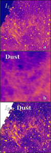 |
Fig. A.1. Example of the problem of using the WISE dust maps to correct for cirrus in the Euclid images. Panel a shows a region of 25′×25′ in the IE band. Panel b shows the corresponding WISE dust map for the region. Panel c shows the result of subtracting the WISE dust map from the IE image. The residual shows cirrus filaments that the WISE map does not capture. |
Appendix B: CICLE and DAWIS BCG+ICL maps
Figure B.1 presents the CICLE (left panels) and DAWIS (right panels) BCG+ICL maps, for each NISP filter, YE (upper panels), JE (middle panels), and HE (lower panels).
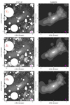 |
Fig. B.1. BCG+ICL maps for the NIR Euclid's YE, JE, and HE bands for CICLE (panels a, c, and e), and DAWIS (panels b, d, and f). |
Appendix C: Colours of cluster members
Figure C.1 shows the YE−JE and JE−HE colour distribution of cluster member galaxies. The colours are taken from the catalogue shown in Sect. 3.3.
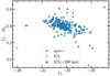 |
Fig. C.1. Colour-magnitude diagram for A 2390 galaxies. Red and gold stars represent the total and the core (r<200 kpc) ICL colour. |
 |
Fig. C.2. Colour distribution of cluster members. |
Appendix D: Stellar population models in the Euclid NIR filters
Here, we explore how the Euclid NIR colours of stellar populations vary with stellar age. In Fig. D.1 we show the NIR colours of the single stellar population models from Vazdekis et al. (2016), assuming a Kroupa (2001) initial mass function, convolved with the Euclid filters, following the prescriptions in Montes et al. (2014). The models are redshifted to the redshift of A 2390 (z= 0.228). The models are colour-coded according to the metallicity, as labelled in the middle panel, and are shown as a function of stellar age. The colour YE−HE, the one used in this paper, of the stellar populations shows almost no variation with age once the stellar ages are >2 Gyr. Therefore, the YE−HE colours in A 2390 are mostly insensitive to age, so we are tracing changes in the metallicity of the stellar populations of the BCG+ICL.
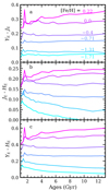 |
Fig. D.1. Euclid NIR colours of the Vazdekis et al. (2016) single stellar population models shown as a function of stellar age, for A 2390. When the stellar population is older than 2 Gyr, its YE−JE (panel a), JE−HE (panel b), and YE−HE (panel c) colours are fairly constant with age but vary with metallicity. |
All Tables
ICL and BCG+ICL fractions and luminosities of A 2390, measured by the different methods explored in this work, namely CICLE, DAWIS, and 1D Profile Ahad.
Properties of the six groups identified by the DS+ method: group identifier, number of members, distance to the centre of the cluster, velocity dispersion, and mean velocity.
All Figures
|
Fig. 1. RGB image of the A 2390 galaxy cluster Euclid FoV. The contrast is greatly enhanced to highlight large-scale colour variations (due to cirrus and background inhomogeneities) across the whole image in the LSB regime. Blue is VIS, green is the JE band, and red is the YE band. North is up and east is to the left. |
| In the text | |
|
Fig. 2. Effect of cirrus removal for all NISP filter images. Left to right: Original image; cirrus+background map; cirrus-corrected image. The angular size of the images is |
| In the text | |
|
Fig. 3. Zoom-in on regions of interest in the YE band, which displays the most cirrus residuals after correction. Top row shows a |
| In the text | |
|
Fig. 4. Top: Mock cluster radial profiles in the HE band before (red) and after (blue) cirrus correction. The true BCG+ICL light profile is shown as a black line. Bottom: Difference between the true BCG+ICL light profile and the measured BCG+ICL profiles. |
| In the text | |
|
Fig. 5. Image of the |
| In the text | |
|
Fig. 6.
|
| In the text | |
|
Fig. 7.
|
| In the text | |
|
Fig. 8. Histogram of background pixels in the three cirrus-subtracted NISP bands. Because the background was also removed during the process, all three distributions are centred close to zero. |
| In the text | |
|
Fig. 9. Surface brightness profiles of the BCG+ICL in the three NISP bands before (top panel) and after (bottom panel) subtracting the residual background. The flux density values are shown with a magnitude zero-point of 30. |
| In the text | |
|
Fig. 10. Surface brightness radial profiles for the BCG+ICL of A 2390 from the 1D method Ahad. Profiles for the YE (orange), JE (red), and YE (dark red) NISP bands are shown. |
| In the text | |
|
Fig. 11. Colour radial profiles for the BCG+ICL system of A 2390. Green diamonds represent the cluster selected members, while red, blue, and green lines are the ICL radial profiles estimated with the three methods presented in Sect. 4: Ahad in blue; CICLE in green; and DAWIS in red. The vertical lines indicate 10 and 50 kpc, to guide the eye. |
| In the text | |
|
Fig. 12. Density map of the 219 galaxies selected as belonging to the cluster A 2390 (see main text). The green contour levels correspond to 3σ, 10σ, and 20σ above the background. North is up and east is to the left. The image size is |
| In the text | |
|
Fig. 13. Contour maps of the spatial distribution of elliptical (red) and spiral (blue) galaxies overlaid on the HE-band image of A 2390 in the upper panel, and the DAWIS BCG+ICL map in the lower panel. The figure shows a region of 700″×700″ (2.5 Mpc×2.5 Mpc) centred on the BCG. |
| In the text | |
|
Fig. 14. RGB images of the BCG+ICL in the core of A 2390 (700 ″×700 ″). The left panel shows the CICLE RGB map and the right panel the DAWIS RGB map. The numbers in both maps mark the position of the galaxies in the groups identified by DS+ (see Sect. 5.4.3), listed in Table 2. Both colour images were generated with Trilogy (Coe et al. 2012). |
| In the text | |
|
Fig. 15. Region of 700″×700″ around A 2390. The background is the ICL filled-contour map from DAWIS (HE band) while the blue and orange lines are the mass and X-ray contours, respectively. The contours are at 50 (lightest shade), 100, 150, 200, 300, 500, 600, 700 kpc (darkest shade). |
| In the text | |
|
Fig. A.1. Example of the problem of using the WISE dust maps to correct for cirrus in the Euclid images. Panel a shows a region of 25′×25′ in the IE band. Panel b shows the corresponding WISE dust map for the region. Panel c shows the result of subtracting the WISE dust map from the IE image. The residual shows cirrus filaments that the WISE map does not capture. |
| In the text | |
|
Fig. B.1. BCG+ICL maps for the NIR Euclid's YE, JE, and HE bands for CICLE (panels a, c, and e), and DAWIS (panels b, d, and f). |
| In the text | |
|
Fig. C.1. Colour-magnitude diagram for A 2390 galaxies. Red and gold stars represent the total and the core (r<200 kpc) ICL colour. |
| In the text | |
|
Fig. C.2. Colour distribution of cluster members. |
| In the text | |
|
Fig. D.1. Euclid NIR colours of the Vazdekis et al. (2016) single stellar population models shown as a function of stellar age, for A 2390. When the stellar population is older than 2 Gyr, its YE−JE (panel a), JE−HE (panel b), and YE−HE (panel c) colours are fairly constant with age but vary with metallicity. |
| In the text | |
Current usage metrics show cumulative count of Article Views (full-text article views including HTML views, PDF and ePub downloads, according to the available data) and Abstracts Views on Vision4Press platform.
Data correspond to usage on the plateform after 2015. The current usage metrics is available 48-96 hours after online publication and is updated daily on week days.
Initial download of the metrics may take a while.