| Issue |
A&A
Volume 698, May 2025
|
|
|---|---|---|
| Article Number | A45 | |
| Number of page(s) | 12 | |
| Section | Cosmology (including clusters of galaxies) | |
| DOI | https://doi.org/10.1051/0004-6361/202553716 | |
| Published online | 28 May 2025 | |
Multi-scale exploration of SMACS J0723.3–7327’s intracluster light and past dynamical history
OCA, P.H.C Boulevard de l’Observatoire CS 34229, 06304 Nice Cedex 4, France
⋆ Corresponding author.
Received:
9
January
2025
Accepted:
1
April
2025
We present an analysis of the intracluster light (ICL) in the galaxy cluster SMACS J0723.3–7327 (hereafter, SMACS J0723) using JWST/NIRCam deep imaging in six filters (F090W to F444W). We processed images for low surface brightness (LSB) science, applying additional corrections for instrumental scattering in the short-wavelength channels. We analysed the images using wavelet-based decomposition and extracted and modelled the ICL, brightest cluster galaxy (BCG), and satellite galaxies, generating 2D maps for each component. The ICL and ICL + BCG fractions, computed in all filters within a 400 kpc radius, exhibit a flat trend with wavelength, averaging 28% and 34%, respectively. Flux ratios between the BCG and the next brightest members (M12, M13, and M14) also display minimal wavelength dependence. These results indicate that SMACS J0723 is a dynamically evolved cluster with a dominant BCG and well-developed ICL. We analysed five prominent ICL substructures that contribute 10–12% of the total ICL+BCG flux budget, slightly exceeding simulation predictions. Their short dynamical timescales suggest an instantaneous ICL injection rate of several 103 L⊙ yr−1, consistent with active dynamical assembly. These findings support a scenario where SMACS J0723’s ICL growth is currently driven by galaxy mergers involving the BCG and other bright satellites, rather than by the accretion of pre-processed ICL from a recent cluster merger. However, extrapolating the current injection rate to the cluster’s lifetime indicates that additional mechanisms are required to match the growth observed in other clusters over cosmic timescales.
Key words: galaxies: clusters: general / galaxies: interactions
© The Authors 2025
 Open Access article, published by EDP Sciences, under the terms of the Creative Commons Attribution License (https://creativecommons.org/licenses/by/4.0), which permits unrestricted use, distribution, and reproduction in any medium, provided the original work is properly cited.
This article is published in open access under the Subscribe to Open model. Subscribe to A&A to support open access publication.
1. Introduction
In the current Lambda cold dark matter (ΛCDM) paradigm, galaxy clusters assemble hierarchically through the accretion of other clusters and groups. During this non-linear process, the galaxies evolving in these dense environments experience many gravitational interactions, with other cluster galaxies or with the cluster potential itself. One outcome of these dynamical interplays is the intracluster light (ICL), a faint (μV ≥ 26.5 mag arcsec−1, Rudick et al. 2006) feature of galaxy clusters emitted by stars bound to the cluster potential rather than individual galaxies (see Montes 2022; Contini et al. 2022, for reviews). Observations of nearby, well-resolved galaxy clusters such as Virgo and Coma provide detailed insight into ICL. The ICL is characterised by a smooth and diffuse halo (Jiménez-Teja et al. 2019) in addition to substructures such as tidal streams (Mihos et al. 2005; Janowiecki et al. 2010; Mihos et al. 2017), plumes (Gregg & West 1998), and curved arcs (Trentham & Mobasher 1998). Each tidal feature represents a remnant of a past dynamical interaction, with its properties – such as shape, morphology, colour, and spatial position within the cluster – encoding information about the timing of the event or the actors involved. Dissecting the ICL and its subcomponents is akin to conducting an archaeological investigation of a cluster’s dynamical history.
Early numerical studies pointed to star tidal stripping by the gravitational potential of the cluster (Byrd & Valtonen 1990) and violent galaxy-galaxy interactions (Moore et al. 1996, 1999) as mechanisms responsible for producing tidal streams in galaxy clusters. Subsequent studies using N-body simulations detailed multiple steps during ICL formation, with the creation of transient, dynamically cold streams, followed by their dissolution into the cluster potential (Rudick et al. 2006, 2009). This process, known as stellar stripping, has been demonstrated to efficiently inject stars into the ICL (Contini et al. 2014, 2018), although the exact physical processes – such as major or minor galaxy mergers or fly-by interactions – and the link to the resulting tidal feature properties remain poorly understood. Advances in computational power have enabled simulations to probe hundreds to thousands of galaxy clusters (Remus et al. 2017; Springel et al. 2018; Pillepich et al. 2018; Nelson et al. 2024), demonstrating the stochastic nature of ICL formation (Contini et al. 2023) and highlighting stellar stripping as the dominant contributor relative to other formation channels (Chun et al. 2023, 2024; Contini et al. 2024). However, the contribution of pre-processing (Mihos 2004) is also significant. Recent studies from Martin et al. (2024), highlight the importance of refined mass resolution in N-body simulations, as poorly resolved dark matter halos can lead to excessive stellar stripping.
Observations have explored the overall fraction, morphology, and colour of ICL in galaxy clusters, from z ∼ 0.1 − 0.5 (e.g. Jiménez-Teja et al. 2018, 2023; Montes & Trujillo 2019; Kluge et al. 2020; Ellien et al. 2019; Zhang et al. 2019; Furnell et al. 2021; Dupke et al. 2022; Ragusa et al. 2023; Golden-Marx et al. 2025; Kluge et al. 2025) and up to z ∼ 1 − 2 (Adami et al. 2013; Joo & Jee 2023). Despite the ubiquitous nature of ICL, key questions remain regarding the importance of different formation mechanisms, the growth rate of ICL with redshift, and its dependence on cluster properties. Tidal substructures are rarely discussed in the literature because they blend into the diffuse ICL for clusters at z ≥ 0.1, due to cosmological dimming and decreased spatial resolution. Recent advances in near-infrared (NIR) instrumentation, particularly with the launch of the James Webb Space Telescope (JWST), provide an unprecedented opportunity to address this gap and improve our understanding of the ICL tidal debris at z ≥ 0.2, as well as their connection to the dynamical history of their host cluster. This opportunity arose with the JWST Early Release Observations (EROs; Pontoppidan et al. 2022) of SMACS J0723.3–7327 (herafter, SMACS J0723), a cluster with a mass of M500 = 7.9 ± 1.1 × 10¹⁴ M⊙ (Finner et al. 2023), at z = 0.3877, which is part of the MAssive Cluster Survey (MACS) sample (Repp & Ebeling 2018). This cluster displays a brightest cluster galaxy (BCG) located at  ,
,  , along with large amounts of ICL, extending up to 400 kpc in JWST images, with several visible tidal features (Montes & Trujillo 2022). By combining multi-wavelength data, Mahler et al. (2023) provides evidence that this cluster may have experienced a recent merging episode, probably on an axis close to our line of sight. Subsequent studies show that while SMACS J0723’s ICL correlates with the globular cluster and dwarf galaxy density distributions (Martis et al. 2024), fine substructures and cavities in the ICL were not found in the dark matter-dominated mass distribution (Diego et al. 2023).
This work focuses on constraining the past and current dynamical state of SMACS J0723 using different markers: ICL fractions, magnitude gap, and tidal stream properties. The open access data used for the analysis are briefly described in Sect. 2. Section 3 details the methods used to model the different image components, the results are shown in Sect. 4 and discussed in Sect. 5. A summary is provided in Sect. 6. A standard ΛCDM cosmology is assumed, with Ωm = 0.3, ΩΛ = 0.7, and H0 = 70 km s−1 Mpc−1. This results in a scale of 5.271 kpc/″.
2. Data
2.1. Near Infrared Camera (NIRCam) images
SMACS J0723 was observed with NIRCam using six filters: short channel (F090W, F150W, and F200W) and long channel (F277W, F356W, and F444W). Although the exquisite sensitivity of the JWST ensures deep photometric limits, the released reduced images were unsuitable for low surface brightness (LSB) astronomy due to instrumental light gradients. For long channel images, Montes & Trujillo (2022) corrected background gradients in individual frames by masking all galaxies, foreground and background objects, and the cluster core. A second-degree 2D polynomial was fitted to the masked frames to model and remove the gradient while preserving the ICL. The background correction was refined through an iterative masking process, before the corrected frames were co-added and a constant background value was subtracted from the final images. The short channel images posed additional challenges due to the detectors being smaller than the cluster’s ICL extent and lacking a common gradient. Instead of fitting a plane, the authors corrected for readout patterns and detector scaling. They first removed low-level electronic noise (‘1/f noise’) by subtracting the 3σ-clipped median value from each row. Subsequently, the four detectors were scaled using a reference detector prior to assembling the final mosaics. The corrected images used in this study are publicly available as open-access data1. Despite the improved pipeline, the short channel images still present 1/f noise residuals as stripe patterns, and Montes & Trujillo (2022) excluded these images from their analysis. In the present study, additional attention is given to further correct for this instrumental background (see Sect. 3.1 and Appendix A).
Because these data were part of the original release (Pontoppidan et al. 2022), photometric calibration systematics were issued for this version of the images (Rigby et al. 2023). As a result, absolute flux values cannot be reliably compared across different filters. To mitigate this limitation, all flux-involved quantities computed and analysed in this work are expressed in dimensionless forms, such as ICL fractions and flux ratios, ensuring consistency despite calibration uncertainties.
2.2. Galaxy catalogue
Several galaxy catalogues of the SMACS J0723 field are already available in the literature. Most notably, Mahler et al. (2023) identified the cluster’s red sequence (RS) using Hubble Space Telescope (HST) F606W and F814W filters, resulting in a catalogue of 144 galaxies. They also independently identified 26 galaxies with spectroscopic redshifts from Very Large Telescope (VLT)/Multi Unit Spectroscopic Explorer (MUSE) data, of which all but four belong to the RS. More recently, Noirot et al. (2023) published a spectroscopic redshift catalogue of 190 sources, measured using combined MUSE, Near Infrared Imager and Slitless Spectrograph (NIRISS) and Near-Infrared Spectrograph (NIRSpec) data. For the present work, galaxy members were extracted from the Noirot et al. (2023) catalogue by selecting sources with redshift within 0.3877 ± 0.01. This resulted in a catalogue of 45 galaxies, of which 38 are already part of the RS identified by Mahler et al. (2023). The final galaxy member catalogue was constructed by combining the 144 galaxies of the RS, the 4 VLT/MUSE galaxies identified by Mahler et al. (2023), and the 7 new members identified by Noirot et al. (2023). The resulting catalogue contains 155 sources.
3. Image analysis
A visual inspection of the NIRCam images of SMACS J0723 immediately reveals the difficulties associated with ICL analysis. The extremely high density of sources results in numerous overlapping light halos, and there is a great variety of shapes and morphologies, including foreground MW star halos and crosses, as well as strongly lensed background galaxies. The ICL does not have a smooth distribution but is highly structured with distinctive features such as several tidal streams. The prior-free2 multi-scale decomposition provided by the Detection Algorithm with Wavelets for Intracluster light Studies (DAWIS; Ellien et al. 2021, hereafter E21) is therefore particularly well-suited to model such complex astronomical fields and decouple the ICL distribution from other light sources.
3.1. Pre-processing
Before applying DAWIS to the images, several processing steps were performed to facilitate wavelet analysis. Using the GNU Astronomy Utilities astwarp routine (Akhlaghi & Ichikawa 2015) the images were rotated by 35°, so that the axes of the image corresponded to the two directions of the 2D wavelet transforms. For consistency and to reduce computing time, the short channel images were also resampled to match the pixel size of the long-channel images. The astronomical field was then cropped with the astcrop routine from a 2215 × 2215 pix2 into a square image of size 2048 × 2048 pix2 (corresponding to ∼680 kpc × 680 kpc at the cluster’s redshift). This size conveniently corresponds to the wavelet scale n = 11, and removing the outskirts minimises effects due to visible differences in noise statistics close to the image’s original border. Finally, the instrumental light background of short channel images was modelled as a combination of a linear sharp-edge component and a large-scale background. This combined background was removed from the images, prior to the wavelet analysis presented in the following sections. After correction, the limiting depth (3σ, 10 ″ × 10 ″)3 of the short channel images decreases to values similar to the long-channel images (∼31 mag arcsec−2), which is an improvement over the limiting depth before the correction (∼28–29.5 mag arcsec−2). A complete description of the methodology used for the instrumental light background and the corresponding images can be found in Appendix A.
3.2. Multi-scale decomposition
Most of the analysis was performed with DAWIS, an automated wavelet-based detection algorithm for LSB astronomy. The algorithm is described in detail in Ellien et al. (2021); here, we summarise the salient points. DAWIS decomposes the image information into light contributions denoted ‘atoms’. The process is performed iteratively, with each iteration following the steps of a multi-resolution vision model (Bijaoui & Rué 1995). Firstly, a wavelet transform is applied to the analysed image. The regions of significant wavelet coefficients are then detected and identified as sources. Finally, the light profiles of the brightest sources (set by a relative threshold τ) are restored from their wavelet coefficients. An attenuation factor γ is then applied to each restored light profile to diminish potential restoration errors, and the resulting restored 2D light profile is referred to as an atom. These atoms are subtracted from the image and the algorithm repeats the process on the residuals upon convergence. The algorithm convergence is controlled by a parameter ϵ (see Appendix B for details of the parameters and their values used in this work).
The output of DAWIS for each image is a list of atoms, the sum of which reconstructs the entire astronomical field. The restored images and residuals for the F150W and F356W filters are shown in Fig. 1. Due to the isotropic B3-spline wavelet used by DAWIS, some bright and/or linear features are not captured as accurately as others. Typically, bright foreground stars (including their cores and diffraction spikes) are excessively restored by the algorithm, leading to overestimation of their flux. This occurs because the algorithm injects too much flux into the individual elements that make up these sources, indicating that additional iterations are required to model their complex structures. Similarly, the cores of some bright galaxies appear overly spread as a result. However, the overall restoration quality is excellent with values below 1% of the average in the residuals (equivalent to differences of the order of 10−5 MJy/sr between the original image and the synthesis image).
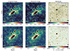 |
Fig. 1. Detection Algorithm with Wavelets for Intracluster Light Studies (DAWIS) outputs for the F150W and F356W filters, shown in the top and bottom panels, respectively. From left to right: original field, complete restored field by DAWIS, and residuals. The size of the images is |

3.3. Atom selection and image synthesis
One atom does not represent an entire astrophysical source, but rather a substructure. This decomposition is artificial and depends on how the signal was captured in the wavelet space at each iteration. However, atoms can be selected to synthesise images that contain the light profile of specific astrophysical sources. The most straightforward case is the sum of all atoms detected and restored by DAWIS, which results in a synthesis image of the entire astronomical field (see previous section).
In this study, several atom properties are used as priors depending on the selection: the wavelet scale ws at which it has been detected (wavelet separation, WS), the coordinates of the local maximum (spatial filtering, SF) and the size Sa (size separation, SS). A wide range of selection schemes and parameter values are applied to produce the following synthesis images for each filter: ICL, ICL+BCG, member galaxy (with and without the BCG), and total cluster (ICL+BCG+satellites) maps. Details about the different selection schemes, the effects of their parameters, and the synthesis of ICL maps are given in Appendix C.
4. Results
Several ICL and ICL+BCG maps were produced using different atom selection schemes. For simplicity, the combined WS+SF+SS scheme with ws = 5 and Sa = 80 kpc was adopted as the main analysis scheme in this work and is discussed here. The rationale for this choice is detailed in Appendix C. The corresponding ICL+BCG maps for each filter are shown in Fig. 4.1. All values discussed here are computed from these maps.
4.1. ICL 2D distribution and fractions
A visual inspection of the models shown in Fig. 4.1 illustrates the complex multi-scale nature of the ICL, featuring an extended 2D distribution over hundreds of kpc spanned by substructures. This complexity is well captured by the DAWIS wavelet modelling. The ICL distribution appears similar in all filters except F090W, where the faint diffuse signal is not as well recovered. Specifically, the F090W ICL+BCG map lacks substructures compared to the other bands, which is expected given that this image has the lowest photometric depth and is most impacted by instrumental light contamination. In each filter, a bright, compact source to the south-east of the BCG can be seen. This signal is neither ICL nor BCG, indicating that some non-ICL and non-BCG atoms can accidentally be included in the model. To address this, we applied a bootstrap procedure on atom selection when making any measurements on the synthesised maps (see Appendix D).
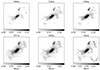 |
Fig. 2. BCG+ICL synthesis maps for each filter resulting from a combined wavelet separation (WS) + size separation (SS) + spatial filtering (SF) scheme with ws = 5 and Sa = 80 kpc. The size of the images is |

The average diffuse ICL distribution is elliptical, with a major axis orientated east-west. The BCG and ICL major axes appear well aligned, with a positional angle in the range 35°–41° in all filters. The ICL ellipticity is higher than that of the BCG in every filter (∼0.26–0.43 compared to ∼0.41–0.57 ). This supports the idea that, while the ICL and BCG are distinct components (Contini et al. 2018), they are correlated and co-evolve, as the transition from the BCG profile to the ICL is continuous. Although the SS criterion applied (Sa = 80 kpc) is consistent with typical values in the literature used to mark this transition (Contini et al. 2022; Brough et al. 2024), it remains artificial and likely does not separate two physical components. This is further supported by the relatively high ICL fractions compared to the ICL + BCG fractions (see the next paragraph).
The ICL (and ICL+BCG) fractions and their error bars were computed for each filter and each selection scheme with the bootstrap procedure described in Appendix D. The resulting fractions for the combined WS+SF+SS scheme with ws = 5 and Sa = 80 kpc are shown in Fig. 3. The ICL and (ICL + BCG) fractions are almost completely flat within the error bars across the six NIRCam filters, with average values of 28% and 34%, respectively. The F090W and F150W fractions appear slightly lower than the others, which can be explained by an over-subtraction of the instrumental light background (see Appendix A), but these differences are not significant considering the error bars. These values are consistent with those found in the visible/NIR bands in the literature for clusters in the 0.1–0.5 redshift range, although they are at the upper end of the distribution (see Fig. 2 of Montes & Trujillo 2022). As different stellar populations would produce different spectral energy distributions, and therefore a variation of the ICL fraction with wavelength, the flat fractions here indicate an intracluster stellar population with similar properties to those of satellite galaxy stars. This suggests that galaxy stripping is the main ICL formation mechanism on the cluster scale. This result is valid regardless of the selection scheme used to produce the map.
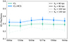 |
Fig. 3. ICL and ICL+BCG fractions for each filter resulting from a combined WS+SF+SS scheme with ws = 5 and different Sa values. |
4.2. Tidal features
A common step in ICL formation through gravitational interactions between galaxies (satellite and/or the BCG) is the creation and subsequent dissolution of tidal features (Rudick et al. 2009). Such features are observed in nearby galaxy clusters, such as Virgo (Mihos et al. 2005, 2017) or Coma (Trentham & Mobasher 1998; Gregg & West 1998), but are generally more difficult to detect at higher redshifts, due to cosmological dimming and lower spatial resolution. Due to the high sensitivity of JWST, SMACS J0723 offers an excellent opportunity to study such tidal features at intermediate redshift, as its ICL is extensively clumpy with prominent overdensities. This analysis focuses on five diffuse substructures with different morphologies and sizes. All are detected in every filter except F090W, where the faint diffuse signal is less well recovered than in the other bands. This suggests that the stellar populations in the tidal features are not very different from those in the average intracluster and satellite galaxy stellar populations and that they originate from galaxy stripping. The positions of these structures are shown schematically in Fig. 4 superposed on the contours of the ICL+BCG map in the F356W filter and satellite galaxy positions. Most of these features were already identified by Montes & Trujillo (2022), namely: the giant west (W) loop, the large north-west (NW) bridge, and the east (E) and south-east (SE) tidal streams. Here, an additional tidal tail to the South (S) of the BCG is identified and denoted as the S tail.
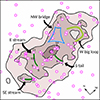 |
Fig. 4. Schematic view of SMACS J0723 stellar content and substructures. The filled contours are drawn from the F356W ICL+BCG map produced by DAWIS. Purple circles indicate satellite galaxies (see Sect. 2.2). Galaxies discussed in the main text are indicated by numbers (1–14, see Sect. 4.2). The main tidal features are highlighted with coloured annotations: the E, SE and S tidal streams are shown in dark green; the external section of the big W loop in light green; and the NW bridge in blue. |
The largest feature is the NW bridge, with an apparent size ∼75 kpc × 50 kpc. It links the BCG (and an interacting satellite in its close halo) with galaxies 1 and 2, the second and third brightest galaxies in the cluster. This indicates that these two massive elliptical galaxies are undergoing strong tidal stripping by the BCG, with a recent close encounter contributing significantly to the ICL build-up. The NW bridge represents 3–5% of the total ICL flux budget across all filters.
The second-largest ICL substructure is the W loop, with a focus here on its outer arc, which spans ∼150 kpc in length and ∼30 kpc in width. To our knowledge, this feature–well aligned with the major axis of the total ICL distribution–is unique because no other loop of this kind has been detected in the ICL of another galaxy cluster. It contributes 2–4% of its total flux budget (except in F090W, where it is undetected and has a negligible budget). Identified as a single stellar stream by Montes & Trujillo (2022), it exhibits a flat colour over kpc scales. However, the origin of the giant loop remains unclear, as it does not appear to be associated with any satellite galaxy. The two large galaxies it seems to be associated with have very different colours (Montes & Trujillo 2022), and are foreground sources that do not belong to the cluster. Satellite galaxies 3 and 4 could be spatially associated with the big loop but are smaller (diameter < 10 kpc) than the loop’s width, excluding them as the main origin for this very large tidal structure. Diego et al. (2023) pointed out that while the cavity is not seen in the total mass 2D distribution, this difference could be attributed to the different nature of the baryonic and dark matter components and result from strong stripping of satellite galaxies following close encounters with the BCG. The dynamical timescale inferred from the mass enclosed in a 200 kpc radius (M200 kpc ∼ 1.5 × 10¹⁴ M⊙, Mahler et al. 2023) is ∼0.2 Gyr. This provides a characteristic decay timescale for tidal streams of ∼0.3 Gyr (Rudick et al. 2009) at these distances from the cluster centre. Assuming that the average distance between the cluster centre and the big loop is 200 kpc (a reasonable assumption, although this radius can vary by a few tens of kpc depending on the part of the loop considered), this suggests that it must have formed recently (< 0.3 Gyr). For the BCG to be at the origin of the big W loop, a collision differential velocity of ∼1000 km s−1 with the other satellite progenitor is required, assuming that the loop retained a similar speed after its creation. This value is well within the range of characteristic velocity dispersions of galaxies in clusters (Goto 2005). Assuming the collision occurred perpendicular to the line of sight and that minimal projection effects are present (a strong hypothesis), the most probable other progenitor is galaxy 14, the elliptical galaxy close to the BCG and currently merging with it.
The E and SE streams have apparent sizes of ∼75 kpc × 15 kpc and ∼40 kpc × 30 kpc, respectively. Neglecting projection effects, the SE stream appears to result from a past encounter between galaxy 12 and galaxy 13. Similarly, the E stream is likely associated with galaxies 8–11. These streams do not contribute as much as the big W loop or the NW bridge to the total ICL flux budget (∼1–2% each), but are textbook cases of stellar stripping through violent encounters between satellite galaxies. Lastly, the S tail also has a relatively small size (∼30 kpc × 10 kpc) and appears to originate from the interaction of galaxies 6 and/or 7 with the BCG. Its morphology appears to be more clumpy than the E and SE streams with patches of stars, indicating a more recent interaction and a less advanced decay state, although it could decay faster because of its proximity to the cluster centre. The light fraction in the S tail relative to the total ICL is similar to that of the streams, with values around ∼1%.
4.3. Magnitude gap
Another way to probe the dynamical state and age of the cluster is by comparing the properties of the BCG with those of the other satellite galaxy members. As the BCG is expected to continuously accrete satellites throughout its lifetime (Solanes et al. 2016), the magnitude differences between the BCG and the second (hereafter M12), third (M13) or fourth (M14) brightest cluster members provide insights into the progress of this build-up (Milosavljević et al. 2006). A large magnitude gap indicates an old, well-evolved system, with a dominant BCG while a small gap points to perturbed and merging systems.
The BCG and second to fourth satellite magnitudes were estimated in each band by integrating the flux from the corresponding DAWIS output models. As stated in Sect. 4.1, the performed separation between BCG and ICL probably underestimates the BCG component. All values discussed here are therefore lower limits on the magnitude gap. For each filter, the measured values for the second and third brightest satellites were found in the range M12 ∼ 1.2 − 1.3 mag and M13 ∼ 1.3 − 1.6 mag. These are galaxies 1 and 2 as indicated in Fig. 4, linked to the BCG by the NW bridge. As discussed in the previous section, these galaxies have probably undergone a past encounter with the BCG, and will likely end up merging with it. The fourth brightest member gap is higher with M14 ∼ 2.3 − 2.5 mag in all filters. The corresponding galaxy is the elliptical galaxy close to the BCG centre and merging with it, as noted by Montes & Trujillo (2022).
Given that these are lower limits, these values indicate a dominant and well-evolved BCG, positioned at the bottom of the cluster potential well and currently accreting a large quantity of matter from its satellites. This is consistent with the high ICL and ICL+BCG fractions measured in Sect. 4.1, as both are linked to the BCG hierarchical assembly and therefore correlate (Golden-Marx et al. 2025).
5. Discussion
5.1. Multiple steps in the ICL formation
It is now widely accepted that the main formation channels of the ICL at z < 1 are pre-processing and galaxy stripping (Contini 2021), with their relative importance depending on the cluster’s current dynamical state. These mechanisms leave distinct imprints on the colour of the ICL. A negative radial colour profile is indicative of an intracluster stellar population following the galaxy morphological segregation, and is therefore associated with the stripping of the outskirts of Milky Way-like galaxies infalling into the cluster (as observed for SMACS J0723 at r > 100 kpc; Montes & Trujillo 2022). In contrast, pre-processing results in local colour variations due to inhomogeneities in the ICL immediately following a major cluster merger, although this is hard to track once the system has had time to relax. Ongoing stripping of galaxies is difficult to observe in images due to the transient nature of tidal streams in galaxy clusters, their LSB, and their low contrast on the diffuse ICL. This dataset therefore provides an excellent opportunity to directly investigate the intermediate steps in the formation of the ICL in SMACS J0723 through the properties of its tidal features.
Together, the tidal features account for approximately 10–12% of the total ICL+BCG budget (∼8% for F090W without the big loop) within a 400 kpc radius. As simulations predict on average 5–10% of the ICL material in stellar streams (Rudick et al. 2009), SMACS J0723 appears to have a high fraction of its ICL in non-relaxed tidal features. All SMACS J0723’s ICL substructures have crossing and decay timescales lower than 0.5 Gyr. The associated star injection rate (the rate at which stars are added to the ICL through dynamical processes) was computed by taking the total flux enclosed in each tidal structure and dividing it by the upper limit of the crossing time (0.5 Gyr). This yielded an averaged star injection rate of the order of a few 103 L⊙ yr−1 in every filter over this period. This is a lower limit, but it remains three orders of magnitude higher than values found in the nearby Virgo cluster (∼ 1 L⊙ yr−1, Mihos et al. 2017), supporting the fact that SMACS J0723 is in the process of building-up its ICL+BCG system, during a phase of strong growth. Assuming this injection rate to be constant throughout the cluster’s lifetime yields a lower limit growth factor of ∼1.7 between 0.1 < z < 0.5. This is slightly lower than the average ICL growth factor of ∼2–4 found in other clusters (Furnell et al. 2021). This is expected, considering that it does not include all ICL injection mechanisms contributing to the growth of the ICL during a cluster lifetime (such as pre-processing and mergers) and indicates that extrapolating the current injection rate to Gyr timescales is likely not valid. Taken together, these results directly support the multiple-step nature of the ICL build-up, with incremental but non-monotonous increases in the ICL fraction over the cluster’s lifetime (Rudick et al. 2006, 2009).
5.2. Dynamical state
ICL fractions in the visible/NIR bands can be used as probes of the cluster dynamical state, although their interpretation should be nuanced by the wavelength at which they are measured. ICL fraction colours with filters probing young stellar populations (Hubble/ACS F606W for example; Jiménez-Teja et al. 2018; Dupke et al. 2022; Jiménez-Teja et al. 2023) are tightly connected to the cluster dynamical state, as recent dynamical mergers result in ICL fraction peaks in these wavelength regimes. This does not hold for the NISP filters as they cover the spectral distribution of stars in the NIR– a wavelength regime that is insensitive to stellar age and instead depends primarily on metallicity. New stars are also expected to be steadily injected into the ICL throughout the lifetime of a cluster, resulting in an overall high-bandwidth ICL fraction for well-evolved, relaxed galaxy clusters (Golden-Marx et al. 2025). The most extreme cases of this scenario are fossil systems (Dupke et al. 2022).
The rather high ICL and ICL+BCG fractions (28% and 34% averaged over all filters, respectively) are therefore indicative of SMACS J0723 being a well-evolved galaxy cluster that had time to build up its ICL. This is supported by the M14 values, typical of evolved and BCG-dominated galaxy clusters, and is consistent with the BCG and X-ray centroid being completely aligned, with signs of cooling in the core of the intracluster medium (Mahler et al. 2023). This scenario is degenerate with another possibility: recent injection of stars into the ICL that increase the ICL fractions (Rudick et al. 2006), as suggested by the presence of many tidal features and a very high current injection rate (see previous section). Considering that the inner (r < 100 kpc) ICL+BCG colours are consistent with a major merger between the BCG and the fourth brightest galaxy (Montes & Trujillo 2022), and that the X-rays feature some inhomogeneities outside the core, SMACS J0723 indeed appears to have undergone recent dynamical activity, possibly a merger with another cluster or group along an axis close to the line of sight (Mahler et al. 2023).
However, a cooling core takes several Gyr to form, a timescale much larger than the decay timescales of the tidal substructures seen in the ICL. Additionally, the ICL fractions do not vary with wavelength, indicating very similar intracluster and galactic stellar populations when considering the cluster as a whole. A major merger with another cluster and its ICL seems therefore unlikely, as stronger perturbations would be seen in the X-ray cluster core. Another probable scenario here is a recent (and still ongoing) internal series of major galaxy mergers between the BCG and the other brightest satellites – a complex grinding phase with strong enough tidal consequences to produce the unique substructures seen in JWST images. These are superimposed on an older, well-mixed ICL diffuse component, fed by previous stripping of the same galaxies experiencing the mergers.
6. Conclusions
In this work, we used the JWST/NIRCam deep images from the original release (Pontoppidan et al. 2022), which focussed on the galaxy cluster SMACS J0723 in six bands (F090W, F150W, F200W, F277W, F356W and F444W) and were processed for LSB science by Montes & Trujillo (2022), to study the ICL in the NIR. Additional care was taken to clean the short channel filters from instrumental scattered light (see Sect. 3.1), and a full wavelet-based decomposition of the images in each band was performed using DAWIS (Ellien et al. 2021). The ICL, BCG and satellite galaxies were all extracted and modelled by leveraging wavelet scale, source size, and spatial position criteria, allowing us to synthesise 2D maps for each component (see Sect. 3).
The ICL and ICL+BCG fractions were computed for each filter using the synthesised maps, displaying a flat trend with wavelength with averages of 28% and 34%, respectively, within a 400 kpc radius. Similarly, the flux ratios between the BCG and the second to fourth brightest members also display flat values with wavelength (M12 ∼ 1.2 − 1.3, M13 ∼ 1.3 − 1.6 and M14 ∼ 2.3 − 2.5 across all filters). These high ICL fractions and magnitude gaps indicate that SMACS J0723 is an evolved galaxy cluster with a dominant BCG and a well-developed, homogeneous ICL.
Five prominent substructures spanning the ICL were also studied: the big W loop, the NW bridge, the S tidal tail, and the E and SE tidal streams. Together, they account for 10–12% of the total ICL+BCG budget within a 400 kpc radius. This is slightly higher than expected on average from simulations (Rudick et al. 2009). Considering the cluster mass, the dynamical timescales of these substructures are a few Myr, resulting in an instantaneous injection rate of a few × 103 L⊙ yr−1, a value much higher than that found in relaxed nearby clusters (Mihos et al. 2017).
Overall, SMACS J0723 appears as a clear example of ICL build-up through episodic growth phases driven by dynamical activity. However, the most probable scenario here is a series of major galaxy mergers between the BCG and the other brightest satellites rather than the injection of pre-processed ICL following a cluster-cluster merger.
Computed in the same way as Montes & Trujillo (2022).
Acknowledgments
Amaël Ellien acknowledges fundings by the CNES post-doctoral fellowship program. This work was made possible by utilising the CANDIDE cluster at the Institut d’Astrophysique de Paris. The cluster was funded through grants from the PNCG, CNES, DIM-ACAV, the Euclid Consortium, and the Danish National Research Foundation Cosmic Dawn Center (DNRF140). It is maintained by Stephane Rouberol. This research made use of Photutils, an Astropy package for detection and photometry of astronomical sources (Bradley et al. 2024). This work was partly done using GNU Astronomy Utilities (Gnuastro, ascl.net/1801.009) version 0.19. Work on Gnuastro has been funded by the Japanese Ministry of Education, Culture, Sports, Science, and Technology (MEXT) scholarship and its Grant-in-Aid for Scientific Research (21244012, 24253003), the European Research Council (ERC) advanced grant 339659-MUSICOS, the Spanish Ministry of Economy and Competitiveness (MINECO, grant number AYA2016-76219-P) and the NextGenerationEU grant through the Recovery and Resilience Facility project ICTS-MRR-2021-03-CEFCA.
References
- Adami, C., Durret, F., Guennou, L., & Da Rocha, C. 2013, A&A, 551, A20 [NASA ADS] [CrossRef] [EDP Sciences] [Google Scholar]
- Akhlaghi, M., & Ichikawa, T. 2015, ApJS, 220, 1 [Google Scholar]
- Bijaoui, A., & Rué, F. 1995, Signal Processing, 46, 345 [Google Scholar]
- Bradley, L., Sipőcz, B., Robitaille, T., et al. 2024, https://doi.org/10.5281/zenodo.4624996 [Google Scholar]
- Brough, S., Ahad, S. L., Bahé, Y. M., et al. 2024, MNRAS, 528, 771 [NASA ADS] [CrossRef] [Google Scholar]
- Byrd, G., & Valtonen, M. 1990, ApJ, 350, 89 [NASA ADS] [CrossRef] [Google Scholar]
- Chun, K., Shin, J., Smith, R., Ko, J., & Yoo, J. 2023, ApJ, 943, 148 [NASA ADS] [CrossRef] [Google Scholar]
- Chun, K., Shin, J., Ko, J., Smith, R., & Yoo, J. 2024, ApJ, 969, 142 [Google Scholar]
- Contini, E. 2021, Galaxies, 9, 60 [NASA ADS] [CrossRef] [Google Scholar]
- Contini, E., De Lucia, G., Villalobos, Á., & Borgani, S. 2014, MNRAS, 437, 3787 [Google Scholar]
- Contini, E., Yi, S. K., & Kang, X. 2018, MNRAS, 479, 932 [NASA ADS] [Google Scholar]
- Contini, E., Chen, H. Z., & Gu, Q. 2022, ApJ, 928, 99 [NASA ADS] [CrossRef] [Google Scholar]
- Contini, E., Jeon, S., Rhee, J., Han, S., & Yi, S. K. 2023, ApJ, 958, 72 [NASA ADS] [CrossRef] [Google Scholar]
- Contini, E., Rhee, J., Han, S., Jeon, S., & Yi, S. K. 2024, AJ, 167, 7 [NASA ADS] [CrossRef] [Google Scholar]
- Diego, J. M., Pascale, M., Frye, B., et al. 2023, A&A, 679, A159 [NASA ADS] [CrossRef] [EDP Sciences] [Google Scholar]
- Dupke, R. A., Jimenez-Teja, Y., Su, Y., et al. 2022, ApJ, 936, 59 [NASA ADS] [CrossRef] [Google Scholar]
- Ellien, A., Durret, F., Adami, C., et al. 2019, A&A, 628, A34 [NASA ADS] [CrossRef] [EDP Sciences] [Google Scholar]
- Ellien, A., Slezak, E., Martinet, N., et al. 2021, A&A, 649, A38 [NASA ADS] [CrossRef] [EDP Sciences] [Google Scholar]
- Finner, K., Faisst, A., Chary, R.-R., & Jee, M. J. 2023, ApJ, 953, 102 [Google Scholar]
- Furnell, K. E., Collins, C. A., Kelvin, L. S., et al. 2021, MNRAS, 502, 2419 [NASA ADS] [CrossRef] [Google Scholar]
- Golden-Marx, J. B., Zhang, Y., Ogando, R. L. C., et al. 2025, MNRAS, 538, 622 [Google Scholar]
- Goto, T. 2005, MNRAS, 359, 1415 [CrossRef] [Google Scholar]
- Gregg, M. D., & West, M. J. 1998, Nature, 396, 549 [NASA ADS] [CrossRef] [Google Scholar]
- Janowiecki, S., Mihos, J. C., Harding, P., et al. 2010, ApJ, 715, 972 [Google Scholar]
- Jiménez-Teja, Y., Dupke, R., Benítez, N., et al. 2018, ApJ, 857, 79 [Google Scholar]
- Jiménez-Teja, Y., Dupke, R. A., Lopes de Oliveira, R., et al. 2019, A&A, 622, A183 [Google Scholar]
- Jiménez-Teja, Y., Dupke, R. A., Lopes, P. A. A., & Vílchez, J. M. 2023, A&A, 676, A39 [NASA ADS] [CrossRef] [EDP Sciences] [Google Scholar]
- Joo, H., & Jee, M. J. 2023, Nature, 613, 37 [NASA ADS] [CrossRef] [Google Scholar]
- Joye, W. A., & Mandel, E. 2003, in Astronomical Data Analysis Software and Systems XII, eds. H. E. Payne, R. I. Jedrzejewski, & R. N. Hook, ASP Conf. Ser., 295, 489 [NASA ADS] [Google Scholar]
- Kluge, M., Neureiter, B., Riffeser, A., et al. 2020, ApJS, 247, 43 [Google Scholar]
- Kluge, M., Hatch, N. A., Montes, M., et al. 2025, A&A, 697, A13 [NASA ADS] [CrossRef] [EDP Sciences] [Google Scholar]
- Mahler, G., Jauzac, M., Richard, J., et al. 2023, ApJ, 945, 49 [CrossRef] [Google Scholar]
- Martin, G., Pearce, F. R., Hatch, N. A., et al. 2024, MNRAS, 535, 2375 [Google Scholar]
- Martis, N. S., Sarrouh, G. T. E., Willott, C. J., et al. 2024, ApJ, 975, 76 [NASA ADS] [CrossRef] [Google Scholar]
- Mihos, J. C. 2004, in Clusters of Galaxies: Probes of Cosmological Structure and Galaxy Evolution, eds. J. S. Mulchaey, A. Dressler, & A. Oemler, 277 [Google Scholar]
- Mihos, J. C., Harding, P., Feldmeier, J., & Morrison, H. 2005, ApJ, 631, L41 [Google Scholar]
- Mihos, J. C., Harding, P., Feldmeier, J. J., et al. 2017, ApJ, 834, 16 [Google Scholar]
- Milosavljević, M., Miller, C. J., Furlanetto, S. R., & Cooray, A. 2006, ApJ, 637, L9 [Google Scholar]
- Montes, M. 2022, Nat. Astron., 6, 308 [NASA ADS] [CrossRef] [Google Scholar]
- Montes, M., & Trujillo, I. 2019, MNRAS, 482, 2838 [Google Scholar]
- Montes, M., & Trujillo, I. 2022, ApJ, 940, L51 [NASA ADS] [CrossRef] [Google Scholar]
- Moore, B., Katz, N., Lake, G., Dressler, A., & Oemler, A. 1996, Nature, 379, 613 [Google Scholar]
- Moore, B., Lake, G., Quinn, T., & Stadel, J. 1999, MNRAS, 304, 465 [NASA ADS] [CrossRef] [Google Scholar]
- Nelson, D., Pillepich, A., Ayromlou, M., et al. 2024, A&A, 686, A157 [NASA ADS] [CrossRef] [EDP Sciences] [Google Scholar]
- Noirot, G., Desprez, G., Asada, Y., et al. 2023, MNRAS, submitted [arXiv:2212.07366] [Google Scholar]
- Pillepich, A., Nelson, D., Hernquist, L., et al. 2018, MNRAS, 475, 648 [Google Scholar]
- Pontoppidan, K. M., Barrientes, J., Blome, C., et al. 2022, ApJ, 936, L14 [NASA ADS] [CrossRef] [Google Scholar]
- Ragusa, R., Iodice, E., Spavone, M., et al. 2023, A&A, 670, L20 [NASA ADS] [CrossRef] [EDP Sciences] [Google Scholar]
- Remus, R.-S., Dolag, K., & Hoffmann, T. L. 2017, Galaxies, 5, 49 [Google Scholar]
- Repp, A., & Ebeling, H. 2018, MNRAS, 479, 844 [NASA ADS] [Google Scholar]
- Rigby, J., Perrin, M., McElwain, M., et al. 2023, PASP, 135, 048001 [NASA ADS] [CrossRef] [Google Scholar]
- Rudick, C. S., Mihos, J. C., & McBride, C. 2006, ApJ, 648, 936 [NASA ADS] [CrossRef] [Google Scholar]
- Rudick, C. S., Mihos, J. C., Frey, L. H., & McBride, C. K. 2009, ApJ, 699, 1518 [Google Scholar]
- Solanes, J. M., Perea, J. D., Darriba, L., et al. 2016, MNRAS, 461, 321 [NASA ADS] [CrossRef] [Google Scholar]
- Springel, V., Pakmor, R., Pillepich, A., et al. 2018, MNRAS, 475, 676 [Google Scholar]
- Trentham, N., & Mobasher, B. 1998, MNRAS, 293, 53 [NASA ADS] [CrossRef] [Google Scholar]
- Zhang, Y., Yanny, B., Palmese, A., et al. 2019, ApJ, 874, 165 [Google Scholar]
Appendix A: Short channel instrumental light background
As stated by Montes & Trujillo (2022), the short channel images were still significantly contaminated by instrumental instrumental light, despite their improved reduction pipeline. This was immediately confirmed by a first run of DAWIS on the images and by synthesizing ICL maps with simplistic selection schemes (see Sect. 3.3 and Appendix C): the ICL was deformed with linear features spatially corresponding with instrumental light stripes. Additional corrections were needed before applying DAWIS to remove this background.
The following empirical approach was performed for each filter: first, a WS synthesised map with all atoms at wavelet planes lower than 7 is created and removed from the original image, leaving a residual image with large-scale variations. These large-scale variations are composed of leftover ICL and the instrumental light background. Here the instrumental light background is approximated by two components: a first component composed of thin stripes giving the sharp details visible in the original images, and a second inhomogeneous large-scale component with different values for each of the four corners corresponding to the four detectors. This second component is first estimated by masking pixels brighter than a 1σ-median threshold (masking sharp edges, most of ICL and some sharp wavelet residuals) before computing an interpolated median background. This first background is subtracted from the residuals, which now contains only ICL leftover and instrumental light sharp edges. Mimicking the correction performed by Montes & Trujillo (2022), a 3σ-clipped median value is computed from each half-row, before performing the same on half-columns. This gives a sharp edge background for each corner of the image, which is then removed. The large-scale background is then reincorporated in the sharp-edge-free residuals, before masking bright pixels once again and performing a new estimation of the large-scale background. Finally, this last background is removed from the images, giving the input images for DAWIS to run again.
The resulting combined background, alongside original, corrected and DAWIS-reconstructed images is shown in Fig. A.2. The improved background is not perfect as some stripe residuals are still visible, mainly in the F090W image. However, these residuals are mainly situated close to the image border and filtered out during the atom selection (see Sect. C). The ICL linear deformations seen before instrumental light background correction are not present in the DAWIS outputs (see fourth column of Fig. A.2) or in the synthesised ICL+BCG maps (see Fig/ 4.1).
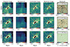 |
Fig. A.2. Outputs from DAWIS for all short channel filters. From left column to right column: original image, instrumental light background, background-subtracted image, restored image (synthesised by summing all atoms detected and restored by DAWIS), residuals (original image with restored image subtracted from). The size of the images is |

Appendix B: DAWIS input parameters
The operating mode of DAWIS is set for all images to standard values with a relative threshold τ = 0.8 and an attenuation factor γ = 0.5, as advocated by E21. The maximum number of wavelet planes explored by the algorithm is set to 10 for long channel images, as their size is approximately 211 pix ×211 pix. The convergence of the algorithm is controlled by a parameter  , with σ(i) the standard deviation of the whole image and nobj, i the number of sources detected and restored at iteration i. Additional details about the form of this parameter are given in E21. However, note that in this work the average of ϵ over the last five iterations is taken for the convergence instead of the individual value for the last iteration. This prevents wrong convergence due to individual iterations where a great amount of flux is detected, restored and removed from the image. For this work, ϵ is set to 10−4 for all images.
Appendix C: Atom selection schemes
Three selection schemes are used in this work to separate atoms based on their properties:
i) Wavelet separation (WS): this scheme performs a separation of atoms based on the wavelet scale at which they are detected. Atoms detected at lower wavelet scales than a given hard limit ws are summed to synthesise a small detail image while atoms detected at higher (ws included) wavelet scales are summed to synthesise a large detail image. Since small sources (typically galaxies) are detected in the first wavelet scales before progressively leaving room to larger structures in lower frequency scales, this scheme allows a first order separation of ICL from smaller structures (E21).
ii) Spatial Filtering (SF): this scheme cross-correlates spatial information (galaxy coordinate catalogue, masks...) with the coordinates of atom centroids to separate them into different components located in different areas of the image. This scheme is used to extract atoms associated to cluster galaxies for example, or again to remove atoms associated to foreground stars.
iii) Size separation (SS): this scheme performs a separation of atoms based on their physical size. Atoms with an x-axis and/or a y-axis size4 smaller than a hard size threshold S are kept as small objects while the others are kept as large objects.
The process of synthesizing images for this work is empirically performed by applying successive combinations of the WS, SF and SS schemes to atoms (the case of the F444W ICL+BCG synthesis image is shown in Fig. C.1 as an example). First, a WS is applied with ws = [3,...,7], allowing a first rough separation of large sources from smaller features. The results are shown in the first line of Fig. C.1. An eye evaluation of the WS synthesis images allows to quickly see that most of galaxy and foreground starlight profiles are removed at ws = 5. However, the low-frequency signal is strongly contaminated by spurious structures such as galaxy/star extended light halos or again extended sources due to the borders of the image.
To remove these contributions a SF scheme is applied on top of the WS. A set of circular masks enclosing the core of foreground stars is created by hand, and atoms with centroid coordinates within these masks are removed completely from the analysis. In the same way, atoms with centroid coordinates outside a large handmade ellipse enclosing the ICL are also removed from the analysis. All atoms detected at wavelet scales lower than ws and with centroid coordinates within a radius of 10 kpc from cluster galaxy coordinates are selected and summed into a cluster galaxy (BCG included) synthesis image. In the case of the ICL+BCG image, the atoms centered on the BCG are simply removed from the galaxy image and added back to the ICL. The results for F444W are displayed on the second line of Fig. C.1.
In addition to the WS+SF model, an SS is added to perform an additional separation of atoms on the basis of their physical size. Contrary to the WS, limited by the amount of wavelet scales used for the analysis, a large number of size thresholds S can be tested to remove/add atoms from the images. In this work a SS is applied to remove atoms with sizes lower than S = [60,80,100,120,140] kpc from the ICL and ICL+BCG synthesis images. The results can be seen on rows 3 to 7 in Fig. C.1.
Due to the fuzzy and ambiguous definition of ICL, one cannot determine exactly which of these models represents best the ICL. However, an eye estimation allows us to see that extreme models are either missing ICL signal (all models with ws = 7) or displaying signal from galaxies (WS and WS+SF models with ws = 3 or 4). By process of elimination, models such as the WS+SF+SS 80 kpc or WS+SF+SS 100 kpc with ws = 5 or 6 are the best candidates to give the most accurate picture of the ICL. For simplicity, only the WS+SF+SS 80 kpc with ws = 5 values are shown and discussed in the main text.
 |
Fig. C.1. Grid of ICL+BCG synthesis models for the F444W filter. The vertical axis shows the name of the models, which are single or combinations of atom selection schemes: wavelet separation (WS), size separation (SS) and spatial filtering (SF). Different versions of the WS+SF+SS model are shown, with a characteristic size varying from 60 to 140 kpc. The horizontal axis shows the different wavelet scales at which the WS is performed. |
Appendix D: Atom selection error
While the synthesized models computed in the previous section are essential to visualize the ICL and get a general impression of its shape, they do not ensure an unbiased estimate of the ICL. The deterministic nature of the reconstruction process of DAWIS does not provide any error bar on the reconstructed atom properties and therefore provides no error bar on more global measurements such as ICL fractions. It does not allow the estimation of atom misclassification (non-ICL atoms included in ICL model, and missed ICL atoms) or the atom resolution of DAWIS (ICL and another source signals can be mixed within a single atom). This is true for the present work, where the high density of overlapping sources in the images leads to some spurious light contaminating the ICL or the satellite galaxy synthesis images (an example is light from the "Beret" galaxy contaminating an overlapping satellite galaxy). Some of these effects can also oppositely influence measurements, resulting in bias compensation (as already highlighted in E21).
To estimate the significance of these effects and to provide error bars, a randomized bootstrap method is applied to each measurement (fluxes, ICL fractions...): variants for each synthesized image are created by randomly adding/removing atoms. Both the number of atoms constituting the image and the atoms themselves can be modified. This allows to probe cases in which ICL is more/less contaminated by spurious sources and cases in which ICL is missing light. Formally, we consider N atoms constituting a synthesized image resulting from a classification scheme and assume two parameters: Pw the percent of ’wrongly classified’ atoms and Pl the percent error on the number of atoms composing the model. First, a new number Ns of atoms is drawn uniformly within [N(1−Pl),N(1+Pl)]. If Ns ≤ N, the atoms composing the new model are drawn from the N original atoms, probing cases where less flux is injected in the model respectively to the classification scheme (under-reconstructed cases). The cases with Ns > N probe instances in which more flux is injected in the model respectively to the scheme (over-reconstructed cases). To emulate contamination, several wrongly classified atoms Nw are drawn within [0,Ns.Pw]. Then Ns − Nw atoms are drawn from the original N atoms, while the Nw contaminants are drawn from atoms that were not selected originally by the scheme (and can therefore include light from foreground/background galaxies or MW stars). This new atom list is then used to produce a variant synthesis image of the selection scheme.
This process is repeated M times, resulting in a sample of M models for each selection scheme. When measuring a quantity for a selection scheme, it is therefore taken as the median of the distribution while the upper and lower errors are computed as the 5th and 95th percentiles. For the rest of this work, Pw = 0.1, Pl = 0.1, and M = 100.
All Figures
|
Fig. 1. Detection Algorithm with Wavelets for Intracluster Light Studies (DAWIS) outputs for the F150W and F356W filters, shown in the top and bottom panels, respectively. From left to right: original field, complete restored field by DAWIS, and residuals. The size of the images is |
| In the text | |
|
Fig. 2. BCG+ICL synthesis maps for each filter resulting from a combined wavelet separation (WS) + size separation (SS) + spatial filtering (SF) scheme with ws = 5 and Sa = 80 kpc. The size of the images is |
| In the text | |
|
Fig. 3. ICL and ICL+BCG fractions for each filter resulting from a combined WS+SF+SS scheme with ws = 5 and different Sa values. |
| In the text | |
|
Fig. 4. Schematic view of SMACS J0723 stellar content and substructures. The filled contours are drawn from the F356W ICL+BCG map produced by DAWIS. Purple circles indicate satellite galaxies (see Sect. 2.2). Galaxies discussed in the main text are indicated by numbers (1–14, see Sect. 4.2). The main tidal features are highlighted with coloured annotations: the E, SE and S tidal streams are shown in dark green; the external section of the big W loop in light green; and the NW bridge in blue. |
| In the text | |
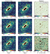 |
Fig. A.1. Same as Fig. 1 but for the long channel filters F277W, F356W and F444W. |
| In the text | |
|
Fig. A.2. Outputs from DAWIS for all short channel filters. From left column to right column: original image, instrumental light background, background-subtracted image, restored image (synthesised by summing all atoms detected and restored by DAWIS), residuals (original image with restored image subtracted from). The size of the images is |
| In the text | |
|
Fig. C.1. Grid of ICL+BCG synthesis models for the F444W filter. The vertical axis shows the name of the models, which are single or combinations of atom selection schemes: wavelet separation (WS), size separation (SS) and spatial filtering (SF). Different versions of the WS+SF+SS model are shown, with a characteristic size varying from 60 to 140 kpc. The horizontal axis shows the different wavelet scales at which the WS is performed. |
| In the text | |
Current usage metrics show cumulative count of Article Views (full-text article views including HTML views, PDF and ePub downloads, according to the available data) and Abstracts Views on Vision4Press platform.
Data correspond to usage on the plateform after 2015. The current usage metrics is available 48-96 hours after online publication and is updated daily on week days.
Initial download of the metrics may take a while.