| Issue |
A&A
Volume 649, May 2021
|
|
|---|---|---|
| Article Number | A38 | |
| Number of page(s) | 26 | |
| Section | Numerical methods and codes | |
| DOI | https://doi.org/10.1051/0004-6361/202038419 | |
| Published online | 07 May 2021 | |
DAWIS: a detection algorithm with wavelets for intracluster light studies
1
Sorbonne Université, CNRS, UMR 7095, Institut d’Astrophysique de Paris, 98bis Bd Arago, 75014 Paris, France
e-mail: This email address is being protected from spambots. You need JavaScript enabled to view it.
2
Observatoire de la Côte d’Azur, BP 4229, 06304 Nice Cedex 4, France
3
Aix-Marseille Univ., CNRS, CNES, LAM, Marseille, France
4
UFRJ, Observatório do Valongo, Rio de Janeiro, RJ, Brazil
5
Independent Researcher, Telschowstr. 16, Garching, Germany
6
Independent Researcher, Est. Caetano Monteiro 2201/65, Niterói, Brazil
Received:
14
May
2020
Accepted:
11
January
2021
Abstract
Context. Large numbers of deep optical images will be available in the near future, allowing statistically significant studies of low surface brightness structures such as intracluster light (ICL) in galaxy clusters. The detection of these structures requires efficient algorithms dedicated to this task, which traditional methods find difficult to solve.
Aims. We present our new detection algorithm with wavelets for intracluster light studies (DAWIS), which we developed and optimized for the detection of low surface brightness sources in images, in particular (but not limited to) ICL.
Methods. DAWIS follows a multiresolution vision based on wavelet representation to detect sources. It is embedded in an iterative procedure called synthesis-by-analysis approach to restore the unmasked light distribution of these sources with very good quality. The algorithm is built so that sources can be classified based on criteria depending on the analysis goal. We present the case of ICL detection and the measurement of ICL fractions. We test the efficiency of DAWIS on 270 mock images of galaxy clusters with various ICL profiles and compare its efficiency to more traditional ICL detection methods such as the surface brightness threshold method. We also run DAWIS on a real galaxy cluster image, and compare the output to results obtained with previous multiscale analysis algorithms.
Results. We find in simulations that DAWIS is on average able to separate galaxy light from ICL more efficiently, and to detect a greater quantity of ICL flux because of the way sky background noise is treated. We also show that the ICL fraction, a metric used on a regular basis to characterize ICL, is subject to several measurement biases on galaxies and ICL fluxes. In the real galaxy cluster image, DAWIS detects a faint and extended source with an absolute magnitude two orders brighter than previous multiscale methods.
Key words: galaxies: clusters: general / methods: data analysis / techniques: image processing
© A. Ellien et al. 2021
 Open Access article, published by EDP Sciences, under the terms of the Creative Commons Attribution License (https://creativecommons.org/licenses/by/4.0), which permits unrestricted use, distribution, and reproduction in any medium, provided the original work is properly cited.
1. Introduction
Low surface brightness (LSB) science will improve in this new decade with the launch of several large observational programs. The Vera Rubin Observatory Large Synoptic Survey Telescope (LSST; Ivezić et al. 2019), a ground-based system featuring an 8.4 m primary mirror, will lead a ten-year survey on a 18 000 deg2 sky area, reaching a foreseen limiting depth of μg = 31 mag arcsec−2. In space, the Euclid mission will perform three deep-field programs in the visible (VIS) broad band (R + I + Z) covering 40 deg2 in total, with a conservatively estimated limiting magnitude of μVIS = 26.5 mag arcsec−2. New missions such as the MESSIER surveyor (Valls-Gabaud & MESSIER Collaboration 2017), a space telescope optimized specifically for LSB imaging in the UV and the visible wavelengths, are also planned for the upcoming years.
These new programs will complement current and past LSB surveys (of which we only give a nonexhaustive review here). Small telescopes optimized for LSB imaging such as the Dragonfly Telephoto Array (Abraham & van Dokkum 2014) or the Burrell Schmidt Telescope (Mihos et al. 2017) are obtaining good results from the ground, reaching limiting depths of μg = 29.5 mag arcsec−2. These small telescopes take advantage of the minimization of artificial contamination sources in a field in which other instruments not originally dedicated to this type of studies are strongly disadvantaged in this regard, such as the MegaCam instrument on the Canada France Hawaii Telescope (CFHT). This last instrument has nevertheless achieved its share of surveys as its limiting depth has been pushed by constraining instrumental contamination effects through refined observational strategies and reduction softwares. The CFHT Legacy Survey (Gwyn 2012) is a good example, as it allowed detecting LSB structures such as tidal streams (Atkinson et al. 2013), followed later by the Next Generation Virgo Cluster Survey (Ferrarese et al. 2012), a survey dedicated to deep imaging of the Virgo cluster. Next in line is the ongoing Ultraviolet Near-Infrared Optical Northern Survey (UNIONS; Ibata et al. 2017), which features images processed with the Elixir-LSB pipeline (Duc et al. 2011) and reaches a limiting depth of μr = 28.3 mag arcsec−2 in the r band on a wide sky area of ∼5000 deg2.
As these ground-based instruments are still limited by the atmosphere, surveys for capturing LSB features have also been led from space with the Hubble Space Telescope (HST), the prime example being the HST Ultra Deep Field (Beckwith et al. 2006). However, the small field of view (FoV) of the HST does not allow probing large spatial extents, leading to different scientific goals such as the study of distant objects that are smaller on the projected sky plane (typically high-redshift galaxies or galaxy clusters). The ongoing Beyond Ultra-deep Frontier Field And Legacy Observations survey (BUFFALO; Steinhardt et al. 2020), next in line to the Hubble Frontier Field (HFF; Lotz et al. 2017), follows this trend and targets six massive galaxy clusters with redshifts in the range 0.3 < z < 0.6 with very deep imaging.
Compared to the ongoing surveys, which are all limited in their own ways, the new generation of telescopes will bring an unprecedented amount of data to exploit. As a subfield of LSB science, the detection and analysis of intracluster light (ICL) will be strongly be affected because one of the primary requirements of studying this faint feature of galaxy clusters in the visible bands is the gathering of deep images. However, the state of research in this field is currently not well defined because there is no consensus on a strict definition of ICL in astronomical images, nor on the best method for detecting it. This leads to a variety of studies on this subject that can be barely compared in view of the large discrepancies implied by the methods that are used (for more details, see the review by Montes 2019). The same can be said about surface brightness depth and the method for computing detection limits from the sky background in images, as explained by Mihos (2019). Before the large upcoming data sets can be efficiently used, a much needed analysis of the currently used detection method properties should be made.
Because part of this new challenge in LSB astronomy is purely technical (processing great numbers of images is often expensive in computing time), new algorithms with an emphasis on efficiency need to be developed to analyze images and to capture the useful information they contain. This is an ideal time to (re)explore concepts from signal and image analysis and adapt them to LSB astronomy. With this in mind, we developed DAWIS, an algorithm optimized for the detection of LSB sources that is highly parallelized and is to be run on large samples of images.
Such a new algorithm needs to be tested on simulations and compared with previous detection methods. To run the tests, we created images of simulated galaxy clusters and ICL using the Galsim package (Rowe et al. 2015). These images only reproduce the photometric aspect of galaxy clusters and cannot be used to draw conclusions on the properties of ICL. However, their content is a known value, which allowed us to estimate the efficiency of DAWIS and of previous methods for detecting ICL. We were also able to constrain the different biases and contamination effects that occur when these methods are applied.
This paper is organized as follows. In Sect. 2 we give some context on the various detection methods that are used to detect ICL in deep images and different effects that limit and contaminate this detection. In Sect. 3 we present the technicalities of DAWIS and the core of the algorithm. In Sect. 4 we describe our simulated mock images of galaxy clusters with ICL with the modeling package Galsim. In Sect. 5 we apply the different detection methods to the simulations and present the results. In Sect. 6 we run DAWIS on real data and compare the results with previous works. In Sect. 7 we discuss the results and the performances of the methods for simulations and real data. We assume a standard ΛCDM cosmology with Ωm = 0.3, ΩΛ = 0.7 and H0 = 70 km s−1 Mpc−1.
2. Overview of ICL detection methods
Behind the term intracluster light detection several choices hide, starting with the way images are acquired (space-based versus ground-based, survey strategies with or without image dithering, long exposures or stacks of short ones), data reduction (depending on the properties of the instrument), and finally, how the useful information is separated from noise and contamination sources (sky background estimation, separation of ICL from galaxies and foreground objects, point spread function (PSF) wings, scattered light). We refrain from addressing all these effects at once, but consider the most fundamental aspect of ICL detection: separating the ICL component from galaxy luminosity distributions and taking the sky background noise into account.
A large variety of methods have been used to separate ICL from bright sources in astronomical images. We group them roughly into three categories: the surface brightness threshold (SBT) methods, the profile-fitting (PF) methods, and the multiscale analysis (usually making use of wavelet bases) methods. The literature knows as many procedures for detecting the ICL as there are papers studying it. This classification therefore simplifies the larger picture, but is probably a good start for characterizing and evaluating this great variety of approaches and ICL definitions.
2.1. Surface brightness threshold methods
The first method is the SBT method, which consists of applying a predefined surface brightness threshold to the image in order to demarcate the ICL from the galaxy luminosity profiles. The most common threshold value is given by the Holmberg radius (defined by the isophote μB = 26.5 mag arcsec−2; Holmberg 1958), which delimits the geometric size of a galaxy in optical images at first order. This threshold has been used in different cases either to mask the cluster galaxies (the threshold in this case defines the limit of the galaxy extension), or simply to separate the outskirts of the brightest cluster galaxy (BCG) luminosity profile from the ICL. In any case, the threshold acts as a decision operator, attributing pixels either to galaxies or to ICL.
This method is quick to implement and has been used in several works (Krick et al. 2006; Krick & Bernstein 2007; Burke et al. 2012; DeMaio et al. 2018; Ko & Jee 2018; Montes & Trujillo 2018, e.g.). Different values for the threshold have been tested (Feldmeier et al. 2002, 2004), resulting in large discrepancies for the results obtained in observational data (Kluge et al. 2020). From the N-body and hydrodynamical simulation side, studies have shown similar results (Rudick et al. 2011; Tang et al. 2018). Depending on the choice of the person performing the study, different SBT values have been tested, with values ranging from μSBT ∼ 23 to μSBT ∼ 27 mag arcsec−2 in the V band, which once again showed strong discrepancies between them. However, because it is difficult to define ICL even in simulations, authors have proposed that different definitions would naturally lead to very different results, without specifying which result is the most appropriate.
2.2. Profile-fitting methods
Intensity PF methods consist of fitting analytical functions to the intensity distribution of the galaxies or to the ICL. The first use of this approach was made by fitting de Vaucouleurs (dV) profiles to the inner intensity distribution of BCGs before excesses of light in the outskirts were detected that were attributed to ICL (Uson et al. 1991; Scheick & Kuhn 1994; Feldmeier et al. 2002; Zibetti et al. 2005). Because the BCG and ICL intensity distributions are smoothly blended, several studies have tried to characterize the BCG+ICL intensity distribution using a single-Sérsic profile (Krick et al. 2006; Krick & Bernstein 2007). Other authors have tried to distinguish the two distributions by fitting sums of profiles, such as double Sérsic (Seigar et al. 2007; Durret et al. 2019; Kluge et al. 2020), double exponential profiles (Gonzalez et al. 2005), or composite profiles (Donzelli et al. 2011). In some cases, different analytical functions can correctly fit the same distribution (Puchwein et al. 2010), which complicates the physical interpretation of such results. Most notably, recent works have sown that the decomposition of the BCG+ICL distribution into separate luminosity profiles is likely unphysical (Remus et al. 2017; Kluge et al. 2020).
Fitting algorithms such as Galfit usually decompose galaxy intensity profiles into two components (bulge plus disk), and allow modeling the radial distribution with Sérsic profiles, while the angular distribution is controlled by trigonometric functions. This allows fitting a great diversity of intensity profiles, as long as the features they present are not too sharp. Most galaxy intensity profiles can therefore be fit with such methods. For complex objects such as strongly interacting galaxies, a high level of interactivity is required, because in these cases the user needs to manually adjust the parameters involved in the fitting procedure. This makes this method difficult to automatize fully, which is a downside when many galaxies are present in the FoV (but not impossible, as shown in Morishita et al. 2017). Additionally, the blending of galaxy intensity profiles in the high-density regions of galaxy clusters is another problem for this type of approach.
Recently, more sophisticated fitting algorithms have been developed, most notably, CICLE (Jiménez-Teja & Benítez 2012; Jiménez-Teja & Dupke 2016). CICLE models galaxy luminosity profiles with Chebyshev Fourier (CHEFs) functions. These forms are implemented into a fitting pipeline using outputs (position and size of the object) from the SExtractor image analysis software (Bertin & Arnouts 1996) because a subjective origin needs to be set for the basis function when each galaxy is modeled. While this fitting method is very strong in accurately modeling the surface brightness distribution of detected objects, it is therefore still sensitive to the detection performances of SExtractor or other detection methods that were used beforehand.
2.3. Wavelets and multiscale image analysis methods
Another approach to the detection of ICL (and generically of faint and extended sources among much brighter objects in astronomical images) has been the use of multiscale wavelet-based algorithms. Isotropic wavelet bases such as the B3-spline scaling function and its associated wavelet transform was used for the first time in an astronomical context by Slezak et al. (1994) to detect the large intracluster medium halo in X-ray images of galaxy clusters. Bijaoui & Rué (1995) then devised a powerful multiresolution vision model to analyze the three-dimensional (3D) data set of wavelet coefficients generated by an isotropic wavelet transform. The related procedure allows detecting significant structures in the 2D wavelet domains, identifying objects in this 3D wavelet space, and restoring the denoised luminosity distribution of these detected structures. This approach enables the detection of extended sources, and can therefore be adapted to the detection of ICL in optical images of galaxy clusters, as demonstrated by Adami et al. (2005). Another known implementation has been the OV_WAV package, developed in 2003 at Observatório do Valongo (OV-UFRJ, Rio de Janeiro) by Daniel Epitácio Pereira and Carlos Rabaça. This IDL package has been used in several works to detect diffuse light in galaxy groups or clusters (Da Rocha & Mendes de Oliveira 2005; Da Rocha et al. 2008; Guennou et al. 2012; Adami et al. 2013). More recently, another implementation of the multiresolution vision model has been developed to process astronomical MHz radio images, adding another deconvolution step and describing the problem within the modern framework of sparse representation (the MORESANE radio astronomical image analysis algorithm; Dabbech et al. 2015). We describe this type of approach and its mathematical background in depth below by compiling and standardizing the various information contained in previous articles.
2.3.1. Choosing a suitable representation space
Beyond the applied algorithm itself, the efficiency of this approach is tightly connected to the mathematical space used to represent the information content of the signal. One way to carry out the detection of the ICL is then to find a new space that highlights the low surface brightness and large spatial extent of the ICL, which facilitates distinguishing it from other astronomical sources.
The mathematical space in which the signal is initially represented (hereafter the direct space) may not be the most efficient for the pursued goal of our our analysis. This can be the case in particular when the information of interest is strongly mixed with other (in that case) components. Identifying a new representation space (and consequently the set of basis functions generating this space) for the data is then of uttermost importance for the final result of the processing. The transform of the initial signal from the direct space to this new space is obtained through inner products with the set of basis functions, defining what is called a projection. Because detecting the ICL in direct space is a difficult task with traditional methods, a more suitable representation space can be sought to facilitate it.
Many basis functions with different regularity properties are available and can define a basis, orthogonal or not. Consequently, as many representation spaces exist. The choice of which basis to use then depends on the signal characteristics that are to be strengthened according to the analysis goals. A generic approach for this choice is the notion of sparsity: an adequate function basis separates the signal of interest from the rest by concentrating the useful information in a few high-valued coefficients while spreading the noise and worthless components to many coefficients with low values. While a sparse representation gathers the relevant information, it may simplify it because features that are very different from the basis functions are lost.
In our case, the typical image of a galaxy cluster in visible bands can roughly be hierarchically decomposed into several circular or elliptical components with different characteristic sizes and intensities: the brightest sources in the FoV are usually PSF-like Milky Way stars and foreground galaxies, then galaxies at the cluster redshift, and finally, faint more distant galaxies, and even fainter extended sources such as the ICL. All are superimposed on a spatially slowly varying (instrumental or not) sky background.
Because their shapes when projected onto the sky are elliptical, a relevant first approach to describing these sources is to use isotropic functions that are azimuthally invariant. Because these sources may have very different characteristic sizes (or spatial frequencies), the function basis also needs to capture localized information (high frequencies) as well as mean behaviors related to the information averaged over a given region of the image (low frequencies). The transform associated with such a basis is called a multiscale transform. It enables studying the signal at varying scales: the transform at small scales gives access to the thinnest and local features of the signal, while its transform at large scales captures its overall behavior. As the analysis goal here is the detection of any feature of interest, an analysis that is invariant under translations would be preferred here. The inner products of the signal with the basis functions then do not depend on the position of the information in the signal, meaning that there is no need to set a subjective origin for the transform, as is the case for shapelets (Refregier 2003).
In our case, an interesting class of functions is the wavelet family. The first- (admissibility condition) and second-order moments of wavelets are equal to zero, making them contrast detectors in the simplest form. An example of such a function is the Morlet wavelet, which is basically a cosine weighted by a Gaussian. A wavelet basis is built by shifting and dilating the same wavelet function (the so-called mother wavelet), and the associated transform is called a wavelet transform. In contrast to the Fourier basis, which gives the most accurate frequency information in an infinite temporal signal in exchange of the loss of date information, wavelet transforms are part of the multiscale transform family. They therefore allow a time-frequency representation because different frequency scales are locally explored by different dilated and translated versions of the same mother wavelet function, providing thereby a date information for each analyzed sample from the whole data set.
The 2D isotropic wavelet bases satisfy the criteria listed above and are consequently adequate at first order to study astronomical images, specifically, images with bright localized sources (the signature in the image of objects such as stars or galaxies) and large diffuse sources (the signature of objects such as intracluster light halos). On the other hand, 2D isotropic wavelet bases are certainly not suitable for detection in image features that are strongly anisotropic or have very sharp edges, such as elongated rectangles or lines (e.g., the PSF spikes around stars, cosmic rays, satellite trails, or tidal debris around galaxies). Any such transform acts as a measure of similarity between the set of wavelets and the studied features. Making use of an isotropic filter implies loose information related to anisotropies, if any. A popular example of a 2D isotropic wavelet function is the normalized second derivative of the Gaussian, nicknamed the Mexican hat (MH) because the shape resembles a sombrero, when used as a 2D kernel: a disk of positive values surrounded by an annulus of negative ones, the integral of which is normalized to zero.
2.3.2. Discretization and multiresolution approach
In order to use wavelet transforms to analyze images, they need to be implemented into algorithms and the continuous theoretical functions along the scales and image axes need to be discretized. A discrete set of functions is built, which may constitute what is called a frame according to the chosen discretization scheme for wavelets with sufficient regularity properties. This discretization is not without consequence because part of the information contained in the continuous function might be lost. An upper limit for the loss of information for a given set of frame bounds, that is, a discretization scheme, can be computed (Daubechies 1990). This loss is small for the MH function when a dyadic scheme and two voices per octave are considered1.
A problem with the MH function though is its extended spatial support – the fact that its profile extends to infinity. It is in practice numerically impossible to compute the exact theoretical transform as approximations need to be done at the edges. Consequently, a widely used MH-like function is the B3-spline wavelet, which is also isotropic and translation invariant with a controlled loss of information when using dyadic scales, but with the prime advantage of having a compact support making the transform computable without any approximation.
A major breakthrough for the understanding and efficient implementation of wavelets into algorithms resulted from the multiresolution theory of Mallat (1989), showing that the set of wavelet functions are no more than a hierarchy or cascades of filters, also known as filter banks in the domain of applying signal processing. Within this framework, the mother wavelets are defined by means of a scaling function, which acts as a low-pass filter. This mother wavelet function in fact appears to be the difference between this scaling function and a normalized version of it dilated by a factor 2 in size. For instance, the MH is the difference between two differently scaled Gaussian functions, and the B3-spline wavelet is the difference between two differently scaled B3-spline functions.
The link between some classes of wavelets (e.g., B3-spline) and filter banks is also expressed through a dilation equation: the scaling function at scale 2 can be expressed as a linear combination of these scaling functions at scale 1. This is true for the continuous basis and for the dyadically discretized version of it. Therefore an image can be iteratively convolved with dilated (and decimated) B3-spline functions using a dyadic scheme, in this way building a set of increasingly coarser approximations of the initial 2D signal. The difference between two successive approximation levels then gives the wavelet coefficients related to this scale range. These coefficients can be viewed as a measure of the information difference between the coarser and thinner approximation, or in other words, of the details in the image with typical sizes within these two scales (cf. bandpass filter).
This iterative approach, which makes use of the so-called à trous algorithm from Holschneider et al. (1989, cf. spatial decimation of the low-pass filters), is much faster than using convolutions with filters of increasing supports to compute the transform. It does not rely on numeric integrals, but benefits from a simplified filtering operator based on simple multiplications and additions. There are different versions of this algorithm depending on the analysis goal. For the 2D decimated wavelet transform, the size in pixels of each smoothed image is divided by four with respect to the previous level of approximation (and so are the number of associated wavelet coefficients). This leads to a pyramidal representation that is well suited to encode the features of the image at a given level with different sizes in a sparse way when these features and the scaling functions match well. An undecimated version has also been proposed, which allows retaining precise spatial information because all the wavelet planes have the same size as the original image. This undecimated wavelet transform with the à trous algorithm and the B3-spline scaling function basis is central to the multiresolution vision model of Bijaoui & Rué (1995), a basic conceptual framework for denoising or source-detection algorithms.
2.3.3. Analysis and restoration
Besides the Haar wavelet, Daubechies has proved (see, e.g., Daubechies 1992) that a wavelet basis cannot simultaneously have a compact support, be isotropic, and be orthogonal. Because the B3-spline wavelet basis has a compact support and is isotropic, its associated representation space is not orthogonal: a source with a single characteristic size in the image is then not to be seen as a set of wavelet coefficients with high values at one single scale, but will have non-null wavelet coefficients at several successive scales. An analysis of the wavelet coefficients is then needed along the spatial axes and the scale axis to link these coefficients and correctly characterize the associated source in the wavelet domain. For the spatial analysis, the undecimated à trous algorithm of Holschneider et al. (1989), first used in the astronomical context in Slezak et al. (1990), and also known as the isotropic undecimated wavelet fransform (IUWT, Starck & Fadili 2007), is easier to use because the various wavelet planes have the same size as the original image.
We briefly explain the properties of the IUWT below, and a rigorous definition is given in Sect. 3.4. According to a dyadic scheme, the image is separated into several scales that exhibit sources with the same characteristic size: the first few high-frequency scales contain compact sources (small-scale details), while the low-frequency scales contain extended sources (large-scale details). Although not perfect because objects in the original image are spread through several sources at different scales, the IUWT is a sparse representation of the initial data. Providing that the noise affecting the data is white, objects in the direct space indeed generate wavelet coefficients with much higher values than those related to the noise-dominated pixels at any except for the smallest scale.
The fact that the IUWT is sparse makes the detection of any faint but extended source much easier in the wavelet domain than in the direct space, especially at the large scales relevant for the ICL component. A hard thresholding of the wavelet coefficients is therefore an efficient way to denoise the data and detect objects or structures, for instance. To do so, the significant wavelet coefficients need to be selected scale by scale and then need to be grouped into connected domains (see Sect. 3.5). Restoring an image in the direct space for a single detected object is slightly more difficult: an interscale analysis must be performed to build interscale trees using the spatial and scale positions of each significant domain, and various constraints can be applied when these trees are built or pruned. The information from a pruned interscale tree can then be used to restore (or reconstruct) the associated object intensity distribution in direct space.
Following the method described in Bijaoui & Rué (1995), only the wavelet coefficients of the domain are used in which the interscale maximum of a tree is located (i.e., the region with the highest value within the tree, hence with the highest information content), and from every region linked to it at smaller scales. This pruning of the interscale trees ensures that the restoration algorithm has access to enough information to compute a satisfying solution, and that the retained information does belong to the same structure in the direct image. However, this pruning discards the information from domains at lower spatial frequencies than the wavelet scale of the interscale maximum. For a source with an intensity profile with an inner core that is much brighter than its outskirts, only the bright core is therefore reconstructed and most of the outskirts are missed. Faint sources near bright ones are therefore correctly processed only when an analysis with such a pruning is performed at least twice.
The restoration step was applied to each tree individually and can be viewed as an inverse problem that yields an iterative estimation process (see Sect. 3.1). Several solutions to such optimization problems have been proposed in the literature, such as conjugate gradient methods or the Landweber scheme (Starck et al. 1998), based on positivity and other regularization constraints. In a more straightforward way, these estimation algorithms aim to reproduce the direct space intensity profile of the detected object by adding and subtracting different elements from a wavelet basis, and using information from the interscale tree. In this paper, the wavelet basis used for the restoration step is usually the same as the basis used for the analysis (the B3-spline wavelet basis).
There are several remarks to make on this overall method. The first is that it is parameter prior-free because there is no need to specify a profile for the objects that are reconstructed, in contrast to usual fitting methods. However, we recall that a choice is made through the wavelet basis that is used for the analysis and the restoration.
Astronomical sources cannot be represented by a single wavelet function, but rather by linear combinations of elements from the same wavelet basis. This implies a selection (made through the estimation algorithm) of the elements of the basis function that lead to the best representation. This selection is performed to minimize the difference in shape between the source intensity distribution and the pattern in the direct space that is linked to the set of wavelet functions that are used to model it. However, this selection is almost always suboptimal, and will generically result in artifacts in the restored profile. In the best-case scenario, the amplitude of these artifacts is very low compared to the other source distribution attributes. Sometimes, however, the iterative process fails to compensate for this difference (and may even amplify it in the worst-case scenario of strongly overlapping objects with high surface brightness), and artifacts can then be significant. Because of the nature of the wavelet pattern, which is a disk of positive pixels surrounded by an annulus of negative ones, these artifacts, if any, in our case take the form of spurious rings around restored sources. Likewise, choosing an isotropic vision model also leads to slight morphological biases on the reconstruction of anisotropic objects, typically galaxies with high ellipticities for which the solution has the same integrated flux but which have a more circular light profile.
2.3.4. Implementation and limitations
A wavelet-based multiscale approach like this was first used by Adami et al. (2005) to detect a large-scale diffuse component within the Coma galaxy cluster. The IDL package OV_WAV is another implementation of this multiresolution approach, and was used to detect diffuse sources in astronomical images of galaxy groups (Da Rocha & Mendes de Oliveira 2005). The wavelet representation allowed the authors to detect extended sources down to a signal-to-noise ratio (S/N) ∼ 0.1 per pixel, which was enough to characterize the intragroup light (IGL) of HCG 15, HCG 35, and HCG 51 (Da Rocha et al. 2008).
Even with fast à trous algorithms, this analysis procedure is computationally time expensive, mainly because of the interscale analysis and the object reconstructions. In addition, a problem met by this approach is the false detections due to statistical fluctuations of the noise. As previously mentioned, the noise is dominant in the high-frequency wavelet scales, and packs of noise pixels with high values can be detected as sources and have their own interscale tree. This results in the reconstruction of incorrect detections in the high-frequency scales, which increases the computing time. The authors of OV_WAV used various ways of thresholding their wavelet scales in order to limit the false detections and applied higher thresholds for the high-frequency scales, but they did not completely solve the problem.
Running OV_WAV on an image allows detecting most of the bright sources and reconstructing them properly up to a very high precision. All the reconstructed sources are then concatenated into a single image: the full reconstructed image of the original field. A residual image can then be computed by subtracting the reconstructed image from the original. Because of the various reconstruction factors described in Sect. 2.3.3, low surface brightness features can be missed. Adami et al. (2005) had the idea of running the algorithm a second time, but on the residual image, in order to detect outer galaxy halos and other more diffuse structures. While better results are obtained in this way, the overall performance of this iterative approach is still determined by the intrinsic quality of the restored intensity distribution for the detected source. This is especially the case for strongly peaked and bright sources because any high-value residual left from the first pass could then be detected as a significant structure in the second pass, once again hiding faint sources that are superimposed or close to it. Ellien et al. (2019) chose this approach for a beta version of DAWIS, where the same algorithm was run three times in a row to correctly detect and model every galaxy in the image. When the ICL is not detected with the wavelet algorithm after this procedure, it is possible as a fast alternative to detect it in the final residual image by applying an appropriate standard sky background threshold. In this case, the wavelet analysis acted as a simple modeling tool for galaxies, analogous to PF methods. A fully iterative procedure with this type of wavelet algorithm is always difficult to apply because of its computational cost, but it appears to be the best way to significantly improve the overall quality of the analysis (especially with regard to object restoration), and to thoroughly detect ICL in the wavelet space.
In parallel to the detection of ICL, this multiscale approach has been adapted to different types of data, where the scientific goals are similar (e.g., detecting faint and extended sources hidden by bright and compact sources). Most notably, Dabbech et al. (2015) proposed the algorithm MORESANE (model reconstruction by synthesis-analysis estimators), developed for processing radio images of galaxy clusters taking the complex PSF of radio interferometers into account. As already said, this algorithm makes use of the multiresolution vision model of Bijaoui & Rué (1995), embedded in an iterative procedure generalizing and upgrading the process implied by the earlier works of Adami et al. (2005) on ICL. This allows solving most of the problems described in the previous paragraphs. Dabbech et al. (2015) also provided a description of the overall procedure and algorithm in terms of sparse representation, called synthesis-by-analysis approach. We decided to use this latest version of multiscale image-analysis procedure as a starting point to upgrade this class of methods for detecting ICL. We propose here our own version of this strategy, optimized for computation time and for optical images. We presented it in the next section.
3. DAWIS
In this section we present the operating structure of DAWIS. While many notions addressed here are already well known, we still detail them with the global understanding of the algorithm in mind. The comparison of the ICL detection performance is presented in Sect. 4. We use the following notations: matrices are denoted by bold uppercase letters (e.g., A with a transpose A⊤), vectors by bold lowercase letters (e.g., v). A component of row index i and column index j is given by Ai, j. A vector component of index i is given by vi. Vectors are all column vectors, and row vectors are denoted as transposes of column vectors (e.g., v⊤). Vector subsets and matrix columns or rows are denoted by top or bottom indexes with parentheses (e.g., v(j) or v(j)).
3.1. Inverse problem and sparse representations
When a signal from observed data is modeled, the solution of this inverse problem may not be unique. To solve this so-called ill-posed problem, a penalty term must be introduced in the mathematical equation that describes it so that a particular solution can be selected. This solution must satisfy this added criterion, thereby leading to an optimization problem. We consider the generic equation
 (1)
(1)
where y ∈ ℝM is the measured signal, x ∈ ℝN is the initial signal, ℋ : ℝN → ℝM is a known (or approximately known) degradation operator, and n ∈ ℝM is an additive noise. This structure can be used to represent many problems in image and signal processing such as denoising with ℋ = I or deconvolution with ℋ an impulse response (i.e., the PSF for a focused optical system). Recovering the initial signal from the observed (sub-)set of data is an inverse problem that can be solved with a penalized estimation process, written as
 (2)
(2)
where ℛ : ℝN → ℝ+ is the penalization function and λ ∈ ℝ+ is the regularization parameter. One widely used constraint is the Tikhonov regularization, which may rely on difference operators, for instance, to promote a smooth solution or the identity matrix to give preference to solutions with small ℓp norms2. Sparsity of the solution for a given representation space can also be enforced. To do so, the penalized function ℛ is then a measure 𝒮 of the sparsity of the solution when projected onto the basis defining this new space, that is, after applying a transform γ to the solution so that the penalty term is written as ℛ(x′) = 𝒮(γ) with γ = γ(x′). This transform γ is usually chosen to be a linear operator. The normalized matrix aggregating the new basis functions as columns is commonly referred to as a dictionary, and each column or vector of it is then an element that is also called an atom.
A natural choice for the function 𝒮 is the ℓp norm with 0 < p < 1 to favor sparsity. Case p = 0 related to support minimization is usually untractable because it is highly nonconvex, hence an NP-hard problem; case p = 1 corresponds to the tightest convex relaxation to this problem, which may still not be easy to solve efficiently when the dimension is high. The use of dictionaries (cf. composite features) in combination with ℓ1 norm gave rise to several minimization algorithms with many variants to determine the best approximation of x by the elements of the dictionary, such as the method of frame (Daubechies 1988), the basis pursuit scheme (Chen et al. 2001), or the compressive sensing (Donoho 2006). Faster than convex optimization but lacking uniformity, a greedy method such as (orthogonal) matching pursuit (Mallat 1993), which is conceptually easier to implement, is also a suitable and efficient algorithm to solve the task.
Recovery of the sparse (or compressible) signal x is guaranteed providing that the correlation between any two elements of the dictionary is small (as measured by the mutual coherence indicator or the K-restricted isometry constant) and the number of measurements is large enough (Candes et al. 2006). In case of overcomplete and redundant dictionaries, the successful restoration of the signal relies on the use of a prior as is often the case for solving many inverse problems, with the maximum a posteriori (MAP) estimator, for instance. The prior we are interested in is the sparsity of the solution we are looking for, and it can be introduced following two approaches that are closely related but not equivalent for such redundant dictionaries, as studied by Elad et al. (2007).
The first approach relies on an analysis-based prior. The signal x characterized by its inner products with all the atoms of a dictionary A is assumed to be sparse for this dictionary, that is, γa = A⊤x with γa the sparse representation of x. To be efficient, this approach must involve priors on the signal for selecting adequate dictionaries such as wavelet-based ones for nearly isotropic sources in astronomical images, as was implemented in the previous algorithm OV_WAV. Given ℓ1(x) = ∑i|xi|, Eq. (2) becomes
 (3)
(3)
The second approach is sparse synthesis, where the signal to be restored, x, is assumed to be a linear combination of a few atoms from a dictionary, so that x = Sγs, where γs is the sparse representation of x and S is the synthesis dictionary (not to be confused with the measure of sparsity 𝒮). This leads to the solution of the inverse problem as
 (4)
(4)
For redundant dictionaries, solutions for analysis or synthesis priors are different. As far as the authors know, no general results on their practical comparison are available for usual transforms, even for the ℓ1 norm case. However, the analysis approach may be more robust than the synthesis approach because it does not require the signal to be expressed as a linear combination of atoms of a given dictionary. It is clear that a synthesis approach with dictionaries including too few atoms leads to a rough restoration and that the number of unknowns for large dictionaries is computationally expensive and often prohibitive.
3.2. DAWIS: A synthesis-by-analysis approach
We chose a hybrid approach for DAWIS, the analysis-by-synthesis method first developed for processing radio astronomy images and explicitly implemented in the MORESANE algorithm (Dabbech et al. 2015). The principle is to model an image as a linear combination of synthesis atoms that are learned iteratively through analysis-based priors. The previous algorithm, OV_WAV, already follows this path implicitly because (i) it makes use of wavelet dictionaries to reconstruct images according to an analysis approach where objects are detected and restored subject to the wavelet coefficient values, and (ii) it sometimes has to be run iteratively two or three times to obtain better results, which is the beginning of a synthesis approach with the successive restored images as synthesis atoms. However, applying a formal analysis-by-synthesis method allows us to solve most of the problems met by the OV_WAV algorithm while keeping the advantages of an analysis based on wavelet atoms for the detection of low surface brightness features.
This approach makes DAWIS (like MORESANE) a very versatile tool with a great range of applications, as the nature of the signal of interest and of the degradation operator are defined by the person performing the analysis. In the work presented here, for example, the signal to be recovered is the ICL, and the degradation operator ℋ can then be seen as effects coming from instrumental (scattered light, PSF) and physical (blending of astronomical sources, contamination by diffuse halos, etc.) origins. However, our goal of using DAWIS here is not to cope with instrumental effects (this type of degradation must therefore have been dealt with before), but to focus on the detection of diffuse and low surface brightness features (e.g., detecting signal where standard detection methods fail) and source separation (e.g., separating the ICL from the galaxies based on nonarbitrary parameters). The operating mode of DAWIS is therefore conditioned by these specific analysis goals. We stress the fact that other applications are possible (also see Sect. 3.10 for more details).
3.3. DAWIS: A semi-greedy algorithm
The synthesis-by-analysis approach implemented in MORESANE by Dabbech et al. (2015) and in DAWIS by us is conceptually reminiscent of a matching pursuit algorithm (Mallat 1993) where the atoms of the dictionary are constructed with orthogonal projections of the signal on time-frequency functions. At each iteration the best correlated projection is kept as an atom for the synthesis dictionary, and retrieved from the signal before the same process is applied to the residual. This method is efficient in determining atoms that characterize the signal well because its core strategy is to minimize at each iteration a residual from the computation of the inner products of the underconstruction solution with all the atoms of the analysis dictionary, hence a so-called greedy method, which has the main disadvantage to be time consuming. A well-known greedy algorithm is CLEAN, which uses a set of Diracs and a PSF to deconvolve the image of a field of stars represented by intensity peaks. The algorithm assesses a Dirac function to each peak with a spatial position in the image and an amplitude, which makes it sparse by nature because the observed field is expressed with a few positive coefficients. The sky image is recovered with the convolution of the set of Diracs by the PSF, which can be seen as the product of coordinates by a dictionary with one single atom.
A problem when detecting sources in astronomical images is blending: a faint source aside a much brighter source is partially hidden by the bright source, especially if the latter is also larger. In CLEAN, an iterative process controlled by an empirical factor called the CLEAN factor is introduced to address this issue. The highest detected peak in the image is first considered, and instead of totally removing it from the image before computing and processing the new highest peak, only a fraction of it given by this CLEAN factor is subtracted. By doing so, the risk of accidentally removing faint blended sources is decreased, hence allowing a better deconvolution of the image.
In DAWIS the brightest source within the image is detected at each iteration in the wavelet space before it is restored and removed from the image. Likewise, a very bright object in the image (such as a foreground star) translates into wavelet coefficients with very high values that strongly dominate this representation space (even at low frequency scales), and contaminates low surface brightness features. Removing this bright structure first before detecting fainter sources allows a better recovery of the objects than in the previous process used in the OV_WAV algorithm. Similarly to MORESANE, we also introduced a parameter δ ∈ [0, 1] in DAWIS that is equivalent to the CLEAN factor so that only a fraction of the reconstructed object is actually removed from the image. This also limits the appearance of artifacts.
The downside of this approach is its slowness. An analysis in which sources are processed one by one is far too time-expensive computationally. We therefore decided for DAWIS to implement the semi-greedy method of MORESANE. The reconstructed atom at each iteration is not composed of a single source, but of a set of sources with similar characteristic sizes and intensities. This set is defined by a parameter τ ∈ [0.1], setting a threshold relative to the brightest structure in the image.
3.4. DAWIS: the B3-spline wavelet as analysis dictionary
We described above that we used an analysis-based method to obtain the synthesized atoms of S. As ICL is believed to have an isotropic or quasi-isotropic shape, we chose as adequate dictionary the well-known B3-spline wavelet dictionary, with w = A⊤x, where w is the vector of the wavelet coefficients. The choice of this symmetric and compact mother wavelet also grants a very efficient way to compute these coefficients using the IUWT, for which there is no need to compute the product between A⊤ and x. Benefiting from the so-called à trous algorithm (Holschneider et al. 1989), the original image x is smoothed consecutively J times using an adaptive B3-spline kernel, giving J coarse versions of x, with c(j) ∈ ℝN being the version at the scale j. The vector w can then be written as the concatenation of J + 1 vectors w(j) ∈ ℝN such as w = {w(1)|…|w(j)|…|w(J)|c(J)}, where w(j) = c(j + 1) − c(j) (Mallat 1989; Shensa 1992). Each vector w(j) basically represents the details of two consecutive smoothed levels, and the components of these vectors are called the wavelet coefficients. An image of size N pixels gives a maximum number of scales J ≤ log2(N)−1.
3.5. DAWIS: Noise filtering and multiresolution support
Determining which wavelet coefficients are of interest (filtering step) requires knowing how the noise in the direct space translates into the wavelet space. Because the wavelet transform is linear, the noise statistics remain the same. To be able to select wavelet coefficients using a simple thresholding method involving Gaussian statistics, we need to ensure such a Gaussian distribution for the noise in the wavelet space. For this purpose, DAWIS makes use of a variance stabilization transform. Considering an image x with a combination of Gaussian noise and Poissonian noise, DAWIS involves the generalized Anscombe transform 𝒜 : ℝN → ℝN (Anscombe 1948), which is given by
 (5)
(5)
with g being the gain of the detector, and μ and σ are the mean and standard deviation of the Poissonian-Gaussian noise in the original image, respectively, computed here with a bisection-like method. The result  is an image with a Gaussian noise of σ = 1, which has a very nice behavior in the wavelet space. The à trous algorithm can then be applied to the output image to create the stabilized wavelet coefficient vectors
  .
.
The statistically significant pixels are then selected at each scale using a thresholding method, and a multiscale support is identified (Bijaoui & Rué 1995), which is given a scalar operator 𝒯, a vector M = {M(1)|…|M(j)|…|M(J)} with M(j) ∈ ℝN such as
 (6)
(6)
The computation of the multiscale support fills two objectives. First, it acts as a ℓ0 sparsification of the analysis coefficients, discarding small (nonsignificant) wavelet coefficients and indicating the position of interesting features. Second, it allows us to very easily translate this acquired knowledge from the variance-stabilized wavelet space into the nonstabilized space (e.g., the vector w generated by A⊤x), where the actual object identification is made.
Because the noise in the initial image is considered to be spatially uncorrelated (which is not always the case in reality) and therefore generates wavelet coefficients with high values only at the first two high-frequency scales, a first relevant approach is to estimate the standard deviation of the noise and its mean at these two first scales. The IUWT being a linear transform, the rms values can then be extrapolated to the higher wavelet scales where (i) the noise becomes highly correlated as a result of the large size of the related filters, and (ii) the mean source size increases, leaving increasingly fewer background pixels to estimate the noise statistics.
The threshold operator applied to the wavelet coefficients 𝒯 can take many forms. DAWIS implements the usual hard threshold operator, which operates as
 (7)
(7)
The threshold t applied to each  is different, such as t = kσ(j), with σ(j) being the standard deviation of the noise of
  and k a constant usually chosen to be 3 or 5 according to the chosen probability for false alarms. Other formulations for 𝒯 can be used, such as the soft threshold operator (Mallat 2008) or the combined evidence operator used in OV_WAV (Da Rocha & Mendes de Oliveira 2005).
3.6. DAWIS: Object identification through interscale connectivity
We first repeat that a source in the original image generates significant wavelet coefficients at several successive scales for a nonorthogonal transform. Consequently, an analysis along the scale axis has to be performed in order to identify the set of wavelet coefficients related to this source. To this end, DAWIS once again follows the recipe first proposed by Bijaoui & Rué (1995) and also implemented in MORESANE. It relies on the construction of interscale trees.
We denote with α the set of significant wavelet coefficients of w. The location of these coefficients is given by the multiscale support M defined in Sect. 3.5. When this mask is applied, a classical segmentation procedure is first performed to group these coefficients into regions (e.g., domains) of connected pixels. α can then be written as a concatenation of vectors α(j) so that α = {α(1)|…|α(j)|…|α(J)} with α(j) ⊂ w(j), each α(j) being composed of a set of domains d with different sizes. As usual, each significant region is characterized by the location and amplitude of its coefficient with the highest value, allowing us to define a local maximum. Let  be this local maximum value for the region d(1) ⊂ α(j). Region d(1) is then defined as linked to a region d(2) ⊂ α(j+1) when
  belongs to d(2). Finally, by testing this connectivity for each region d ⊂ α, interscale trees are built throughout the whole segmented wavelet space.
With this procedure, an object O is then defined by the concatenation of K connected regions in the wavelet space d(k) such as O = {d(1)|…|d(k)|…|d(K)}. A region is linked to at most one other region at the next lower frequency scale, but can be linked to several regions at the next higher frequency scale. One criterion must be satisfied to consider that such a tree is related to a genuine object in the direct image, and not an artifact. An interscale tree must include at least three regions that are linked at three successive scales.
3.7. DAWIS: Object reconstruction
Applying the procedure summarized in the previous section, each object in direct space is therefore related to an interscale tree of significant wavelet coefficients. Beyond the structure of the tree itself, the amount of information about this object is distributed throughout the linked regions and can be measured by the value of their maxima once normalized. Because wavelets act as a contrast detector, the average values of the wavelet coefficient amplitudes tend to be indeed lower at small scales than at large scales in astronomical images, thereby creating an implicit bias when wavelet coefficient values at different scales are compared. As a normalization factor for each scale j, DAWIS uses the standard deviation at this scale j of the IUWT of a Gaussian white-noise image with unit variance, denoted  . For an object O, this results in the normalized vector
  of size K, with given d(k) ⊂ α(j),
  .
.
The region d(k) ⊂ O in the tree that contains most of the information about the object is especially relevant for the information content. This region of maximum information is the interscale maximum. It is denoted by an index kobj and a scale jobj such as
 (8)
(8)
This interscale maximum gives an easy way to characterize an object O because the parameter jobj provides its characteristic size 2jobj. Moreover, the parameter  giving its normalized intensity is also used by DAWIS to compare it to other objects and rank them for the restoration step. As indicated in Sect. 3.3, a parameter τ defines a threshold relative to the brightest identified object, which has the highest parameter
  , denoted
  . Only objects for which
  are restored at a given iteration of the processing and are included in the associated dictionary atom.
Objects are reconstructed individually, using their specific support Mspec giving the location in w of every significant coefficient belonging to O. Here DAWIS also strictly follows the procedure of Bijaoui & Rué (1995) and that regions at scales j higher than jobj are discarded for the restoration. This restoration is a direct application of Eq. (2), where positivity of the solution is used as a regularization term, with y = Mspecw and ℋ = MspecA⊤. DAWIS uses the conjugate gradient algorithm from Bijaoui & Rué (1995), which makes use of the adjoint operator †A of the analysis dictionary A (see their article for an explicit definition of this operator). This algorithm iteratively finds the solution  , which is the reconstructed object. This conjugate gradient version algorithm makes use of the Fletcher-Reeves step size β (Fletcher & Reeves 1964). This process is applied to all objects before they are concatenated into a single restored image z ∈ ℝN such as
  .
.
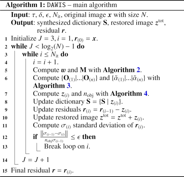
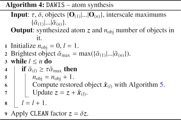
3.8. DAWIS: Architecture of the algorithm
We present the general architecture of DAWIS in the form of a simplified pseudo-code in this section: Algorithms 1 and 4 summarize the synthesis-by-analysis approach as explained in Sects. 3.2 and 3.3, while Algorithms 2, 3, and 5 describe the wavelet-atom-based analysis as described in Sects. 3.4–3.7. For the operating mode of DAWIS, which is iterative, some parameters have to be defined to control the convergence of the algorithm.
To ensure that the algorithm correctly peels the image starting by the bright sources, we imposed an upper scale J so that the brightest detected object at each iteration cannot have an interscale maximum  at scale jmax > J. This also decreases the computation time because there is no need to perform the wavelet and interscale analyzes for all scales for the first few iterations. The upper scale is initialized at J = 3 because an interscale tree needs domains that are connected at least at three successive scales to be considered as related to an object.
The main convergence parameter is defined as  and is computed from the variation of the standard deviation of the residual at each iteration i. However, the nature of the synthesis atom for different iterations can induce instability for this convergence parameter. One atom can indeed be composed of many bright objects, which means strong variation in the standard deviation, and another of a single faint object, hence a low variation in the standard deviation, which might break the loop while there are still sources in the residual. Therefore we normalized this convergence parameter by the number of objects nobj to stabilize it. When the value of this parameter decreases below a threshold ϵ, the value of the upper scale J is increased by one, so that larger sources can be processed by the algorithm. A hard limit Nit is also given to the algorithm to restrict the number of possible iterations.
3.9. DAWIS: implementation and parallelization
DAWIS is implemented with an emphasis on modularity (e.g., a set of modules that can be moved or replaced by new versions) because the algorithm can still be upgraded to increase the quality of the method or modified according to new analysis goals. We chose to write the main layer of modules in Python because it is a very widely used versatile and accessible open-source language. However, this versatility has a cost in terms of numerical performance, which led us to support the Python modules by Fortran 90 codes where the main numerical computations are done.
Input: Maximum scale J, residual r.
Output: wavelet coefficients w and multiscale support M.
-
Apply Anscombe transform
 .
. -
Compute
 with à trous algorithm for scale j = 1 to J.
 -
Apply hard threshold
 .
. -
Compute multiscale support M from
 .
. -
Compute w = A⊤r with à trous algorithm for scale j = 1 to J.

As explained in Sect. 2.3.4, one of the main limitations of wavelet-based algorithms is computation time, which prevents the application of previous packages such as OV_WAV to large samples of images or to very large images. Great effort has been made with DAWIS to parallelize the algorithm. This is not straightforward because the main algorithm is iterative, which means that only the content of one iteration can be sped up. Therefore we parallelized the modules inside an iteration. When large data arrays are worked (which is typically the case when the wavelet data cube and the multiresolution support are computed with Algorithm 2 and when the multiscale analysis is performed with Algorithm 3), the Fortran modules are parallelized in shared memory using OpenMP3. Conversely, we use the new Python package Ray4 to distribute processes when we work on many small arrays (the restorations of numerous objects to compute the associated synthesis atom are independent from each other and can be distributed, such as Algorithms 4 and 5).

We display here a central processing unit (CPU) computing-time scaling test on mock data for both types of parallelizations. For the shared memory parallelization, the test was set on an image of size 4096 × 4096 pixels (giving a wavelet data cube of 4096 × 4096 × 10 wavelet coefficients). Algorithms 2 and 3 were run on the image first serially (one CPU), and then with progressively increasing the number of CPUs. As shown in Fig. 1, the gain of computing time is high when the number of CPUs is increased from 1 to 16: it changes from a computing time of ∼40 min to a computing time of ∼6 min. However, these modules do not scale linearly with the number of CPUs, and the gain in computing time is rather negligible for 32 and more CPUs, where the computing time converges toward a value of ∼4 min.
 |
Fig. 1. CPU computing-time scaling test for the two types of parallelization used in DAWIS. The scale for the computing time is logarithmic. This gain in time is achieved for the modules inside one main iteration of the algorithm, and does not represent the total CPU computing time of DAWIS (see the text for more details). |
For the distributed memory parallelization, the test was run on 1000 copies of the same object array of size 128 × 128 pixels. Algorithms 4 and 5 were run on the arrays, and the resulting CPU computing times are also displayed in Fig. 1. Similar to the shared-memory parallelization, the gain in CPU computing time is most effective when the number of CPUs is increased to 16, for which the computing time changes from ∼25 min to ∼2 min. It is rather negligible with higher numbers of CPUs, however, and converges toward a computing time of ∼2 min. The objects that are to be restored are not always of size 128 × 128 pixels, and the number of objects that is to be restored can also differ from 1000. In some cases, the object sizes might even be a large fraction of the image. In these cases, however, there are rarely more than one or two objects that need to be restored. In our experience, the computation time of an iteration with one or two large objects that are to be restored does not differ very much from the computation time of an iteration in which many small objects are restored.
This simple test is not representative of the performance of the complete algorithm. Because of the greedy nature of Algorithm 1, the CPU computing time of DAWIS largely depends on the content of the image. An image that contains complex structures will always take longer to process than an image with very simple shapes because more main iterations are needed to accurately model these complex structures (in our experience, the number of main iterations ranges from a hundred to a few hundred, depending on the image). Additionally, the length of a main iteration also greatly depends on the content of the image. For example, the algorithm will sometimes choose to restore only one very bright source. In this case, the parallelization in distributed memory is of no use because only one object is to be restored. Nevertheless, these parallelization processes ensure that the complete CPU computing time of DAWIS does not disproportionately increase in case of ‘heavy’ main iterations.
3.10. Astrophysical priors on object selection
We showed in Sect. 3.2 that the columns of the final synthesized dictionary S are atoms that are no more than the restored images zi at each iteration i. Then, the restoration ztot of the whole original image is given by the sum of all these atoms such as ztot = ∑iz(i). The generic operating mode of DAWIS therefore produces a fully (denoised) restored image every time the algorithm is run. However, in this way, a large part of the information recovered by the sparse synthesis-by-analysis method is not used because all synthesized atoms are concatenated into the same image in which the information of individual spatial frequencies or characteristic sizes is no longer accessible. However, depending on the analysis goals, the subsets of atoms of S alone might be of interest, or even more specifically, alternative synthesized dictionaries might have to be compiled, the atoms of which would be selected differently throughout the synthesis-by-analysis procedure. To allow for these possibilities, a discrimination operator 𝒟 was applied to the detected objects before we constructed the associated synthesis atoms such as  . We do not present a rigorous definition of such an operator here because it can take many forms and use different properties to distinguish objects depending on the desired goal.
In this paper, the main goal is to detect the bright components characterizing ICL. The discrimination operator 𝒟 then becomes a way of classifying sources as ICL-type structures, denoted  , and to extract them from components associated with galaxies. A very simple way of doing so is to consider jobj for each object and to use this parameter as a constraint because the characteristic size of galaxies is not the same as the characteristic size of any structural element of the ICL. The dictionary atom zICL can then be built in parallel of z such that
  . This atom is then added to the ICL-synthesized dictionary SICL, and a fully restored ICL image can be computed by summing all its atoms. A distinction based on the spatial position of the interscale maximum kobj can also be applied because atoms describing galaxies belonging to a galaxy cluster would also be considered (a catalog of the cluster member positions is needed in this case) for ICL fraction studies, for example, or again to ensure that atoms associated with ICL are well centered on the galaxy cluster. More complete discrimination operators can be developed based on morphological properties of sources in the wavelet scales, for instance, granularity (i.e., the number of regions linked to an interscale maximum), depth of the interscale tree (i.e., the number of scales composing the tree), or the color of the restored object (when several bands are available).
4. Simulations
A new detection algorithm such as DAWIS must be tested and compared to more traditional methods. For this purpose, we took an image analysis approach and created monochromatic mock images of galaxy clusters simulated with the Galsim package (Rowe et al. 2015), emulating the photometric aspect of galaxy clusters (galaxies + ICL) and the properties of the CFHT wide-field camera MegaCam. The choice of MegaCam was made to prepare upcoming ground-based surveys such as the UNIONS survey (Ibata et al. 2017). However, the same approach can (and should in the future) be applied to simulations of HST images, for example.
From an astrophysics point of view, this approach is not the most realistic because the simulated images contain only light profiles and an artificial background. However, it allows a complete control over the different included components and allowed us to compare different detection methods and their performances in different situations. Even if they are more realistic, it is not possible to repeat this with N-body or hydrodynamical simulations because the way in which ICL is defined in those simulations is also subject to debate (Rudick et al. 2011; Tang et al. 2018).
4.1. Photometric calibration
We retrieved the MegaCam properties on the MegaPrime website5. The MegaCam-type images are set with a pixel scale s = 0.187 arcsec pixel−1, a detector gain g = 1.62e−/ADU, an exposure time texp = 3600 seconds, and a readout noise level σreadout = 5e−. We calibrated the photometry for the r band with a zeropoint ZP = 26.22, and set the sky surface brightness μsky to the corresponding average dark sky value, which is μsky = 21.3 mag arcsec−2. The sky background level in ADU/pix is then given by
 (9)
(9)
The sky background in our images was simulated using the Galsim function ‘CCDNoise(sky_level =  , gain = g, read_noise = σreadout)’, which generates a spatially flat noise composed of Gaussian readout noise plus Poissonian noise.
We neither tried to model the MegaCam PSF and the associated complex scattered light halos in a refined way nor to measure the effect of its extended wings, and we did not include any spatial variation or anisotropy to it. We therefore chose a constant value for the seeing. We modeled the PSF with a Moffat profile using the Galsim function ‘galsim.Moffat’ with parameters β = 4.765 and a half-light radius of 0.7″, which is a generic value for the MegaCam seeing.
4.2. Creating catalogs
We first created a galaxy cluster catalog. Because the vast majority of ICL detections in the literature was made at low redshift (z < 0.5, with a few exceptions such as Adami et al. 2005; Burke et al. 2012; Guennou et al. 2012; Ko & Jee 2018), we picked three redshift values such as z ∈ [0.1, 0.3, 0.5] in which ten different galaxy clusters per bin were simulated. This choice of redshift values was made to study the effect of cosmological dimming on the ICL detection for each detection method. While the number of clusters per bin seems at first fairly low, different parameter spaces for each cluster ICL profiles were explored by multiplying the number of processed images to several hundred and allowing us to lead a statistically significant study.
A Navarro-Frenk-White (NFW; Navarro et al. 1997) dark matter (DM) gravitational potential was simulated at the center of an image for each cluster. The mass of the potential was set to an average value of 1015 M⊙, and its concentration followed the N-body simulation concentrations of Klypin et al. (2016). Recent works have shown that the spatial distribution of ICL should follow the concentration of the DM halo (Montes & Trujillo 2019). This was not the case in our simulations, and we did not explore the effects of the mass and concentration parameters on our results. Our goal was to mimic the photometric aspect of galaxy clusters and their ICL, and not to determine the physical properties of their gravitational potential or the effect of these parameters on ICL.
Galaxy catalogs for each cluster were simulated by drawing galaxy properties (redshift zgal, half-light radius rh, apparent magnitudes in the RC band mRC, and the ellipticity parameters ϵ1 and ϵ2) from the COSMOS 2015 catalog (Laigle et al. 2016) following a Poissonian distribution. First, a homogeneous field of galaxies was generated following the COSMOS 2015 field galaxy luminosity function (GLF) normalized by the size of the simulated image. When the galaxy field was set, the cluster members were also drawn from the COSMOS 2015 catalog, but this time specifically following the GLF in the same redshift bin as the cluster redshift. The field GLF number counts were rescaled with the projected 2D mass density profile of the cluster, so that the number counts reflect those of the cluster rather than those of the field. By doing so, we assumed a constant mass-to-light ratio in the cluster. Galaxy distances to the center are imposed by the cluster mass profile, but their position angles were chosen randomly.
These galaxy catalogs do not reflect all the galaxy cluster properties such as the morphological segregation or the actual surface distribution of galaxies in a cluster (which is usually not exactly proportional to a NFW halo), but they represent typical galaxy clusters at optical wavelengths fairly well: an overdensity of galaxies that spatially follows a halo mass profile superimposed on randomly placed field galaxies. Because the position or the fraction of elliptical and spiral galaxies in the cluster images are not expected to affect the detection of ICL in a significant way, we did not add any supplementary properties to the catalogs. We did not include foreground stars in our simulations either because we tried to estimate the different ways in which galaxies can be separated from ICL in galaxy clusters and not the effect of strong contamination sources such as these stars. Another missing component in these catalogs is a BCG at the center of the galaxy cluster, which was later added by hand (see Sect. 4.3).
We chose a size for the images and the galaxy catalogs of 383 × 383″, corresponding to images of 2048 × 2048 pixels for images like those from the CFHT MegaCam images. This size is very convenient because DAWIS can be run on a statistically significant sample of these images while giving an exact limit of J = 10 on the number of wavelet scales (see Sect. 3.4).
4.3. Generating galaxy light profiles
The galaxy luminosity profiles were generated using the modeling package Galsim in a way similar to Euclid collaboration (2019). Galaxies were represented by a Sérsic profile and drawn into the images using the function ‘galsim.Sersic’. The input half-light radius rh was taken from the catalogs computed in Sect. 4.2, and the value of the Sérsic index n was drawn randomly following a uniform distribution with n ∈ [0.5,5.5]. The input flux in ADU of each galaxy was computed with the relation
 (10)
(10)
with g being the detector gain, texp the exposure time, ZP the zeropoint of the image, and mgal the galaxy magnitude from the catalogs computed in Sect. 4.2. The ellipticity of each galaxy was then computed with the function ‘galsim.Shear(e1 = ϵ1, e2 = ϵ2)’. Each galaxy profile was also convolved with the instrument PSF (see Sect. 4.1) using the function ‘galsim.Convolve’.
To compute the flux of a cluster, we retained only its galaxies within 350 kpc from its center. Applying a physical scale cut allowed us to compare different redshift cases coherently. This ensured that there was no redshift bias when we computed the total flux of a cluster because low-redshift galaxy clusters display a larger apparent size than high-redshift galaxies. Real galaxy clusters are usually much larger, with sizes up to a few megaparsec, but the measure of ICL fractions is dependent on the spatial extent that is probed and on the number of cluster members in it. We therefore imposed this physical radius as a membership constraint, which was also chosen so that the equivalent image radius of clusters in the redshift bin z = 0.1 (r ∼ 189.8 ″, the largest radius of the three redshift values) fits in CFHT MegaCam-type images of 2048 × 2048 pixels. The flux of a galaxy member was then added to the total flux of the galaxy cluster Fcluster, which was then used to compute the ICL luminosity profile.
A BCG was also simulated in the middle of each image by simulating a Sérsic profile. The BCG flux FBCG was computed by taking the flux of the brightest galaxy of the image and applying a cosmological dimming factor corresponding to the cluster redshift to it. This was done by multiplying its flux by a factor (1 + z)4 corresponding to the initial redshift value of the galaxy, and then dividing it by the same factor, but instead with the cluster redshift value. In order to avoid cases in which a very bright foreground galaxy is drawn into the image, which results in a value for FBCG that is too high, we added the constraint that the absolute magnitude of the BCG is not brighter than −23. Following values from the literature (Gonzalez et al. 2005; Seigar et al. 2007; Durret et al. 2019), the BCG Sérsic index was drawn from a uniform distribution in the conservative range [1.5,5.5], and FBCG was added to the cluster total flux  . We assigned the same ellipticity to the BCG as we applied to the ICL light profile generated in the next section.
4.4. Generating the ICL light profile
The procedure of simulating an ICL luminosity profile in a galaxy cluster is relatively unknown, with a variety of biases in the literature due to the various recipes that have been applied to detect it in real images, and because ICL can show different morphologies from cluster to cluster and when the observation wavelength is changed. This is true for the smooth component of ICL, without even mentioning other substructures (tidal streams, shells, etc.). Another unknown area is the fact that there is still no meaningful proof that the stellar populations emitting the ICL and those that compose the galaxies can be separated in a consistent way without star kinematic information and using only photometric data. However, for simplicity we assumed that the ICL has its own light profile and we chose to simulate a large exponential ICL profile with no substructures for each cluster. While this may not be the most realistic approach, it allowed us to probe at first order how the different detection methods we tested act to separate a simple but faint and extended source superimposed on small bright objects. In addition, several studies (Gonzalez et al. 2005; Seigar et al. 2007; Durret et al. 2019) found that the best fits for BCG+ICL systems were usually two-component fits with an internal Sérsic profile and an external profile (exponential or Sérsic, depending on the study).
The ICL profile was simulated using the Galsim function ‘galsim.Exponential(half_light_radius =re, flux  )’. In order to obtain a profile that agrees with the cluster in the same image, we computed the ICL flux in ADU from the total cluster flux
  as
as
 (11)
(11)
with  the input ICL fraction in our images. In the literature, the measured ICL fractions of galaxy clusters at intermediate redshifts usually range from 0.1 to 0.4 (Montes & Trujillo 2018; Jiménez-Teja et al. 2018). Based on these values and because part of our simulated profile is masked by the sky background and the measured ICL fractions will always be lower than the input ICL fractions in our images, we set
 ![Mathematical equation: $ f^{\mathrm{input}}_{\mathrm{ICL}}\in\left[0.2, 0.4, 0.6\right] $](/articles/aa/full_html/2021/05/aa38419-20/aa38419-20-eq41.gif) .
.
While the amount of flux in the ICL profile is controlled by the input ICL fraction, another driver parameter for the profile average surface brightness is the half-light radius re because it controls the concentration of the profile: while a very extended profile would likely fall below the sky background level, a profile with the same input ICL fraction but with smaller re would stand out above. The measured half-light radii from the literature cover a very wide range because they strongly depend on the nature of the study and the quality of the applied fitting method, and the values range from a few dozen to several hundred kiloparsec in the most extreme cases (Gonzalez et al. 2005; Kluge et al. 2020; Durret et al. 2019). In addition and as stated in Sect. 4.3, the characteristic size of our galaxy clusters is set by a physical radius of 350 kpc from the cluster center, giving an intrinsic upper limit in our simulations for our choice of values for re because an ICL profile with a larger half-light radius would make no sense. This led us to set re = [50,100,150] kpc, a range of values probing quite concentrated ICL profiles (50 kpc) and extended ones (150 kpc).
As the effects of the cosmological dimming, the re parameter and the  parameter on the ICL surface brightness are degenerated, we show in Fig. 2 ICL surface brightness radial profiles with different sets of values for these parameters to illustrate their effect. We also display the typical 3σ detection limit in our images for a better visualisation (see Sect. 5.1 for details on how the detection limit was computed). We note that concentrated profiles (re = 50 kpc) display surface brightnesses brighter than μ = 26.5 mag arcsec−2 in their inner parts and could be qualified as ‘unrealistic’, but we nevertheless included them in the study. We also note that some ICL profiles fall completely below the detection limit, making it difficult for traditional detection methods to characterize them.
 |
Fig. 2. Evolution of integrated radial ICL profiles with input ICL fraction, redshift, and half-light radius computed from one of the simulated galaxy cluster catalogs. The typical 3σ detection limit (computed from an image containing only CCD noise) in our MegaCam type images is also displayed as a dashed black line. The half-light radius re controls the concentration of the profile, and the redshift z and the input ICL fraction fICL control its amplitude, with a stronger effect from fICL. Because the detection of ICL is strongly background limited, the outskirts (or the totality in some cases) of the profiles fall below the detection limit and are lost. This loss is estimated in Sect. 5 (also see Fig. 6). |
To summarize, we simulated ten galaxy clusters per redshift bin, and for each of them we varied the re and  parameters in three bins each, giving for each cluster nine different images corresponding to nine different ICL profiles. Because we also wished to ensure a diversity of morphologies for the ICL, we applied a shear to each elliptical profile with the function ‘galsim.Shear(e = ϵ, beta=θ)’ with ϵ the magnitude of the shear in the Galsim distortion definition drawn in the range [0.0,0.8] and θ the angle of the shear drawn in the range [0,180] degrees, both following a uniform distribution. For consistency, the same shear was applied to the nine different galaxy cluster ICL profiles (see Fig. 3 for an example showing the nine MegaCam images of one of the clusters at z = 0.1).
 |
Fig. 3. Mock MegaCam images of a simulated galaxy cluster at redshift z = 0.1 with different ICL light profiles (the cluster is the same as was used for Fig. 2). The concentration of the profile is controlled by the half-light radius re, and its amplitude is controlled by the input ICL fraction fICL. The green circle is the radius rin = 350 kpc, delimiting the core of the cluster. At this redshift, it covers almost the entire image. The intensity scale is logarithmic to highlight the faint ICL halo. |
4.5. Drawing images
We drew a full set of 270 MegaCam-type images using the parameters of Sect. 4.1. In parallel to the generation of these generic cluster images (hereafter GAL+ICL+NOISE), we created alternative MegaCam-type images of these clusters: images containing only the galaxies and the noise (GAL+NOISE), and images containing only the ICL and noise (ICL+NOISE). These alternative versions allowed us to constrain the contamination due to the superposition of galaxies and ICL and the limitations of the different detection methods tested in Sect. 5. Another type of MegaCam-type image was generated during this step specifically for the PF method (see Sect. 5.2 for details). In total, we analyzed 270 different GAL+ICL+NOISE MegaCam-type images with a great diversity of ICL light profiles in morphology and in flux. We also analyzed the equivalent 270 ICL+NOISE MegaCam-type images and 30 GAL+NOISE MegaCam-type images (as there are 30 different galaxy cluster catalogs), making a total of 570 images, which allowed us to statistically evaluate the efficiency of the three detection methods we tested.
5. Applications of detection methods
In this section we describe and apply three different methods to detect ICL in the simulated images of galaxy clusters from Sect. 4. The methods are labeled as follows: surface brightness threshold (SBT), ideal profile-fitting (PF), and DAWIS. We applide the following procedure to each detection method:
-
Application of the method to the ICL+NOISE MegaCam-type images to separately measure the ICL flux, hereafter
 .
. -
Application of the method to the GAL+NOISE MegaCam-type images to separately measure the flux of cluster galaxies, hereafter
 .
. -
Computation of the ICL fraction
 . Comparison of the results with input values to constrain the method limitations.
 -
Application of the method to the GAL+ICL+NOISE MegaCam-type images to measure the fluxes FICL and Fcluster.
-
Computation of fICL = FICL/(FICL + Fcluster). Comparison of the results with
 ,
,  and
and  to constrain the effect of the superposition of galaxies and ICL.
5.1. Surface brightness threshold
We chose to consider a threshold μSBT = 26.5 mag arcsec−2 on our images to constrain this approach and compare it to other detection methods because this value is still the most frequently used in the literature (we also tried different threshold values, as displayed in Appendix A, but only describe the case μSBT = 26.5 mag.arcsec−2 in detail). The procedure is straightforward: for the GAL+ICL+NOISE image, pixels with values brighter than this SBT (taking cosmological dimming for the threshold into account) were masked (their pixel values were set to zero). The pixels included in rin and with values greater than the 3σ detection limit (computed by applying a sigma-clipping algorithm on an image containing only the CCD noise generated in Sect. 4.1) were defined as significant and were associated with ICL. FICL was computed by summing their values. The pixels with values brighter than μSBT were grouped into regions of pixels. A cross-correlation between the catalog of cluster member positions and the position of the pixel with the highest value of each newly defined region of pixels is performed. Matching regions were identified as cluster members and the fluxes of the cluster galaxies Fcluster were computed by summing their values.
This method has a few intrinsic limitations. First, part of the ICL light profile is lost below the 3σ detection limit in the original image, and another part is lost as it is masked by galaxies. The detected ICL flux is also contaminated by galaxy flux from the outskirts of galaxies falling below μSBT (see Fig. 4, where a quick assessment by eye shows this effect) and from undetected galaxies below the 3σ detection limit. To constrain these effects, a similar procedure was applied to the images with separated galaxies and ICL.  was computed from pixels with values brighter than μSBT in the GAL+NOISE image. Because we wished to constrain the loss of ICL flux masked by galaxies, the same masks were applied to the ICL+NOISE image (therefore masking part of the ICL light profile). After this, when any pixels were left that were brighter than μSBT in the ICL+NOISE image, we also masked them because part of the ICL profile might be brighter than this threshold and also masked with galaxies.
  was then computed from the significant pixel values above the 3σ detection limit. Therefore the difference between
  and
and  gives the effect of the masks and of the background noise on the quantity of ICL detected, while the difference between
  and FICL gives the effect of galaxy contamination.
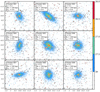 |
Fig. 4. GAL+ICL+NOISE MegaCam-type images of nine galaxy clusters with varying surface brightness thresholds (the color bar indicates the surface brightness threshold: 26 ≤ μSBT ≤ 28 mag arcsec−2). We display here clusters with generic ICL profiles (half-light radius of re = 100 kpc, input ICL fraction of fICL = 0.4, and a redshift z = 0.1) with different ellipticities. The pixels with μ < 26 mag arcsec−2 as well as the non-significant pixels below the detection limit are masked (e.g., white). The galaxy Sérsic profile outskirts contaminating the detection of ICL are easily discernible by eye everywhere in the image when the threshold used to mask galaxies is too bright. In the same way, part of the ICL profile is accidentally masked with galaxies when the threshold is too faint. |
We emphasize the fact that in the literature, studies using this method to separate ICL from galaxies in observational data applied a first pass to extensively mask foreground objects and avoid contamination from bright sources as much as possible before applying the SBT (Burke et al. 2015; Montes & Trujillo 2018, for two examples), using, for example, the SExtractor package. We did not apply such a first pass here. On the one hand, applying this method could lead to stronger contamination effects in the detection of ICL in our simulations. On the other hand, relative to the quantity of actual ICL flux in the image, more ICL is expected to be detected in our work because the spatial area that is degraded by masks is smaller.
5.2. Profile-fitting
The second detection method is based on the galaxy intensity PF, where the fitted profiles are removed from the image before ICL is detected in the residuals. The result of this method strongly depends on the quality of the fits and on the quality of the analysis package used to perform the analysis (packages such as Galfit or CICLE; Peng et al. 2002; Jiménez-Teja et al. 2018). Here again there is a large variety of studies that are different from one another, and we did not try to exactly replicate each of them. Our approach here was to consider an ideal PF method in which the fitting algorithm allows perfectly recovering the intensity profile of each detected galaxy. While it is unlikely that such an algorithm exists or will ever exist, it gives an upper limit to the quality of fitting methods and allows us to compare them easily with other approaches.
The procedure for this method was different from the other two because we did not use exactly the same GAL+ICL+NOISE image. Instead, in parallel of the drawing of the galaxy light profiles in Sect. 4.3, we applied the 3σ detection limit (the same as in Sect. 5.1) to each drawn galaxy, and galaxies without any pixel above this limit were defined as undetected. Every undetected galaxy was added to the generic GAL+ICL+NOISE image (used for the two other detection methods) and to a second image in which we only drew these faint galaxies. The ICL profile and the noise (see Sect. 4.4) were then also added to this image. This image has the same properties as the generic GAL+ICL+NOISE image but without the light profile of detected galaxies, as if a fitting algorithm were able to perfectly remove them. The ICL flux FICL for this method is detected in this image by applying the detection limit to it and keeping the significant pixels included in rin. The cluster galaxy flux Fcluster was computed directly from the light profiles that were not drawn onto this image. With this method, the detected cluster flux is the same for the GAL+NOISE image as for the GAL+ICL+NOISE image, Fcluster =  .
.
Even when the light profiles of galaxies are perfectly removed from the image, this method is still sensitive to galaxy contamination from undetected galaxies that are below the 3σ detection limit. It is also sensitive to the loss of ICL flux below the 3σ detection limit. To constrain these effects, we computed  by summing the values of significant pixels above the 3σ detection limit in the ICL+NOISE image. The difference between
  and
and  gives the amount of flux lost below the detection limit, and it can be compared with the value from the SBT method, which gives the amount of flux lost below the detection limit and behind the galaxy masks. The difference between
  and FICL then gives the amount of ICL flux that is contaminated by faint undetected galaxies with this method, which can once again be compared with the values from the SBT method, where unmasked outskirts of galaxies and undetected faint galaxies contaminate FICL. We also recall that a real PF method would have ICL flux contaminated by residuals, and we did not consider this effect here.
5.3. DAWIS tuned parameters
The detailed operating structure of DAWIS has been explained in Sect. 3, and we provide some additional information about a few parameters here. Various values for the CLEAN factor δ and the relative threshold parameter τ were tested for the MORESANE algorithm, and Dabbech et al. (2015) suggested values τ ∈ [0.8,0.9] and δ ∈ [0.1,0.2] for a good convergence of their algorithm in parallel with a good quality of source restoration. However, their tests were run on more complicated simulations than our mock images of galaxy clusters; the fact that all the sources in our mock images are quasi-circular and the absence of unreasonably bright objects such as foreground Milky Way (MW) stars simplifies the analysis in our case. We set τ = 0.9 and δ = 0.5, a higher value that boosts the convergence of DAWIS slightly. The same values as for these parameters were used for all the processed images.
In order to measure ICL fractions in the GAL+ICL+NOISE images with DAWIS, we need to identify the objects related to ICL and those related to cluster members, and to compute the associated synthesis atoms (see Sect. 3.10). At each main iteration, each object going through the restoration step goes through a two-step selection. First, a cross-correlation between the interscale maximum spatial position of the object and the cluster galaxy catalog was performed. When the wavelet scale of the interscale maximum jobj was greater or equal to a value jsep (corresponding to objects with characteristic sizes of at least 2jsep pixels; we set jsep = 5 for the GAL+ICL+NOISE MegaCam-type images) it was associated with ICL, otherwise it was associated with the cluster galaxies. In this way, we computed in parallel to the total restored image ztot (containing the ICL and all galaxies) the total restored image of cluster members and the total restored image of ICL. A sample of galaxy clusters is shown in Fig. 5 to illustrate the operating mode of DAWIS. FICL and Fcluster are given by the sums of the pixels of their respective images.
 |
Fig. 5. Sample of a few galaxy clusters processed by DAWIS. The clusters are at z = 0.3, and the input ICL profile parameters are re = 100 kpc and |

The main limitation of this approach comes from this very rough classification based on characteristic size. To constrain this limitation, we also ran DAWIS without any classification on the ICL+NOISE image to measure  and on the GAL+NOISE image to measure
  . The first can be compared with the values from the two other methods to show the efficiency of DAWIS in detecting faint sources because it is not limited in the same way by the 3σ detection limit in the original image. Then the difference between
  and FICL, as well as that between
  and Fcluster, shows the effect of the atom classification.
5.4. ICL and galaxies in separated images
We first analyze the results of each method on the ICL+NOISE and GAL+NOISE images. We computed for each cluster and for each method the relative biases,
 (12)
(12)
and
 (13)
(13)
with  the flux of the cluster galaxies measured in the GAL+NOISE image and
  the flux of ICL detected in the ICL+NOISE image.
The values of  for the different detection methods are displayed in Fig. 6 as a function of the various ICL light profile parameters. We first address the results for the PF method, which show in this particular case the amount of ICL flux lost below the 3σ detection limit (also see Fig. 2). As expected, the loss of flux is minimal for concentrated and bright ICL profiles. The brighter the ICL profile, the more it stands out above the sky background. This is best shown by the case with re = 50 kpc and
  , where the values of
  are lower than ∼0.2 at all redshifts for the PF method. This means that less than 20% of the input ICL flux injected in the ICL profile is lost below the 3σ detection limit in that case.
 |
Fig. 6. Relative biases |


For fainter and more extended profiles, the portion of ICL flux that is hidden below the 3σ detection limit is higher. The relative bias  for the PF method reaches strong values such as ∼0.9 for the faintest and most extended profiles (z = 0.5, re = 150 kpc and
  ), meaning that about 90% of the input flux injected in the ICL profile is not detected in this case.
In comparison to the PF method, the  values for the SBT method are always higher. This means that the SBT method detects consistently less ICL flux than the PF method. This is expected because it is not only background limited, but also features a second degradation source of the ICL profile because of the masks. This difference is highly amplified for concentrated and bright profiles (re = 50 kpc and
  ) because this part of the ICL profile is brighter than the SBT threshold μSBT = 26.5 mag.arcsec−2 (see Fig. 2) and is therefore masked.
Of all three methods, DAWIS performs the best: in most cases,  is lower than ∼0.2, with an outlier at 0.4 for the most extended and faintest profile (z = 0.5, re = 150 kpc and
  ). This clearly shows the efficiency of the wavelet-based analysis in detecting faint and extended sources, even when they mostly lie close to or below the usual 3σ detection limit in the original image.
Figure 7 displays the values of the relative bias  . For all methods
  increases with redshift because cluster galaxies become fainter, which decreases the number of detections and results in a loss of detected flux. As expected, the best method here is the PF method because the flux of the cluster galaxies
  is computed directly from the galaxy profiles that are not drawn in the image (see Sect. 5.2 for more details). The bias in this case comes alone from the faint undetected galaxies below the detection limit. This effect is rather weak because
  for the PF method is lower than 0.1, meaning that this effect accounts for a loss of less than 10% of the input flux of the cluster galaxies.
 |
Fig. 7. Relative biases |

The second best performing method on average is DAWIS. The mean  values are lower than 0.2 at all redshifts. However, the error bars show discrepancies between different clusters at the same redshift. The method that performs least is the SBT method with values of ∼0.3 or higher for all redshifts. This is also expected as the Holmberg radius defining the threshold μSBT = 26.5 mag arcsec−2 is only a rough estimate of the galaxy size. This method misses the outskirts of the Sérsic profiles, in addition to flux from faint undetected galaxies.
When Figs. 6 and 7 are compared, the relative bias on ICL  is on average higher than the relative bias on the cluster galaxies
  for the PF and SBT methods. At z = 0.5, for example, both methods disclose
  values lower than 0.4. For faint and extended profiles at the same redshift (z = 0.5, re = 150 kpc and
  ), the
  are twice this value. This shows that these standard detection methods are more limited by the detection of the ICL profile than by the detection of galaxies. In constrast, DAWIS is more stable and discloses equivalent values lower than 0.2 at all redshifts for
  and
and  .
.
The resulting ICL fractions  for separated galaxies and ICL are displayed in Fig. 10 with dashed lines. When we compare our previous analyses of
  and
and  , DAWIS on average measures
  better than the two other detection methods. For bright and concentrated profiles (re = 50 kpc and
  ), the loss of ICL flux due to masking with the SBT method is very significant and results in a large underestimation of
  . This shows that the SBT is the worst method for detecting ICL in this case. On the other hand, the PF method obtains excellent results for the same ICL profiles and performs even better than DAWIS. For faint and extended ICL profiles (re = 150 kpc and
  ), the SBT and PF methods converge on the same results and greatly underestimate the ICL fraction
  .
.
However, while the results of the SBT and PF methods appear to be similar for these faint and extended ICL profiles, Figs. 6 and 7 showed that the measures of  and
and  for both methods are different. The SBT method detects less ICL flux than the PF method, which is compensated by the fact that it also detects less galaxy flux. For the first time in this work, this illustrates that a bias on the measure of ICL flux can compensate for a bias on the measure of cluster galaxy flux when ICL fractions are computed. An amplified version of this effect is shown in the next section, where the contamination effects due to the superposition of galaxies and ICL are discussed.
5.5. Results on superimposed galaxies and ICL
We now show the results of the three detection methods on the GAL+ICL+NOISE MegaCam-type images. We measured FICL and Fcluster in these images, and computed the following relative biases
 (14)
(14)
and
 (15)
(15)
which shows the effect of superposing galaxies on ICL. We call it the contamination effect. The values of  are displayed in Fig. 8. We first consider the values of
  for the PF method. All the values are negative, meaning that more flux is detected and associated with ICL in the GAL+ICL+NOISE image than in the ICL+NOISE image. This shows the contamination effect by faint undetected galaxies because it is the only difference between the measure of
  and FICL. This effect increases with redshift because an increasingly higher number of cluster galaxies falls below the 3σ detection limit. For faint and extended ICL profiles (z = 0.5, re = 150 kpc and
  ), this contamination effect becomes prominent. The value of
  reaches values of almost minus unity, meaning that in this case FICL is twice as high as
  and that the undetected galaxies account for half of the detected flux associated with ICL. In comparison to the PF method, the values of
  for the SBT method show the effect of galaxy outskirt contamination (see Fig. 4 for visualisation) in addition to the contamination effect of faint undetected galaxies. The values are also always negative, meaning that with this method, more flux is detected and associated with ICL in the GAL+ICL+NOISE image than in the ICL+NOISE image. The first problem to address are the very high bias values of this method. We had to truncate them to fit them in the plots of Fig. 8, as
  reaches values of −10 for faint and extended profiles (z = 0.5, re = 150 kpc and
  ). This means that the values of FICL are ten times higher than the values of
  . This shows the very strong contamination effect of galaxy outskirts in this case, which completely dominates the detected flux associated with ICL with the SBT method. The detection of ICL in these cases can be qualified as highly incorrect.
 |
Fig. 8. Relative biases |


DAWIS discloses disparate values for  . The bias is positive on average, showing that less ICL flux is detected in the GAL+ICL+NOISE image than in the ICL+NOISE image. This means that the superposition of ICL and galaxies decreases the amount of flux DAWIS is able to detect and restore. This is expected because DAWIS detects and restores the brightest objects in the image first (the galaxies). Therefore the residuals of these bright sources degrade the detection of the ICL. Additionally, the rough separation based on jsep shows limitations for concentrated profiles (re = 50 kpc). As their characteristic size is smaller, the inner part of these bright and concentrated ICL profiles is not classified as ICL, but as galaxy. This leads to higher bias values than for the extended profiles. The values of
  are displayed in Fig. 9. For the PF method, the values of
  are always equal to zero because the measured flux Fcluster is equal to
  (see Sect. 5.2 for details). For DAWIS, the bias values are also very low. In contrast with the values of
  , this shows that the superposition of galaxies and ICL has little effect on the restoration of galaxies, as explained in the previous paragraph. The method that returns meaningful
  values is the SBT method. The contamination effect of ICL masked with galaxies is strongly seen for bright and concentrated ICL profiles (re = 50 kpc and
  ), and once again, we had to truncate the bias values to fit them into the plot.
 |
Fig. 9. Relative biases |

The resulting ICL fractions fICL are displayed as continuous lines in Fig. 10, together with the ICL fractions  previously computed from the ICL+NOISE and GAL+NOISE images. First, we address the differences in values of
  and fICL for each method. The greatest discrepancies are seen for the SBT method. As previously shown, this is mainly due to the coaddition of several contamination effects: galaxy outskirt contamination, undetected faint galaxies, and ICL partially masked with galaxies for bright and concentrated profiles (re = 50 kpc and
  ). This gives SBT fractions fICL that are systematically higher than their
  counterpart, and even higher than
  for low-input ICL fractions (
 ). This behavior also unveils the fact that some of the apparently accurate fICL values measured by the SBT method are misleading because the detected flux associated with ICL does not come from the actual ICL profile, but in the vast majority from contamination effects. Because they are integrated values, the measured ICL fractions in these cases are close to the input fractions, but these are coincidences due to the set of input parameters. This shows once again an effect of bias compensation, where the flux belonging to ICL is not detected but is replaced by flux from galaxy outskirts.
 |
Fig. 10. ICL fractions displayed for the different ICL profile parameters (half-light radius re, input ICL fraction |


For the PF method, fICL is very close to the  values at low redshift, especially for the bright and concentrated profiles (re = 50 kpc and
  ). It is increasingly higher with redshift, however, giving even higher values than
  at z = 0.5. This is caused by the faint undetected galaxy contamination effect, which is the only effect that contaminates this method. In the same way as the SBT method, the apparently good fICL measured for faint and extended ICL profiles at high redshift are therefore also inflated by contamination effects. However, the PF method is the best-performing method for bright and concentrated profiles (fICL = 0.6 and re = 50 kpc). The measured fractions then decrease when re increases because the method is still background limited and that faint and extended profiles have a higher tendency to be hidden under it. The performance of this method is therefore strongly dependent on the surface brightness of the ICL profile, and gives a good estimate of how much the flux lost below the 3σ detection limit affects the measurement of ICL fractions.
In the case of DAWIS, the atom classification effect is strongly seen for bright profiles (re = 50 kpc and  ) because the values of fICL are lower than the
  values by a factor two. Once again, the effect of the rough classification is strongly seen for these profiles, even in the measure of fICL. DAWIS performs best for extended ICL halos, even for very faint ones because the wavelet analysis, in contrast to regular detections in direct space (original image), uses a spatial correlation to detect sources. The top row DAWIS fractions are therefore better (less contaminated, see
  in Fig. 8) than the other methods, showing its capacity to detect faint and extended features.
6. Example on real astronomical data
In this section we demonstrate the capabilities of DAWIS on a galaxy cluster image at optical wavelengths. The targeted galaxy cluster is LCDCS 0541, which is part of the Las Campanas Distant Cluster Survey (LCDCS; Gonzalez et al. 2001) and the Dark energy American French Team/French American DArk energy Team (DAFT/FADA; Guennou et al. 2010) surveys. The redshift of this cluster is 0.542, and a deep 2 × 2 arcmin2 HST Advanced Camera for Survey (ACS) image in the F814W filter is available. The photometric depth of the image was estimated (Guennou et al. 2012, hereafter G12) to be around μF814W ∼ 24 mag.arcsec−2 for extended sources with SExtractor (∼1.25 arcsec, 1.8σ detection limit). Details about the data and the reduction procedure are available in G12.
We chose LCDCS 0541 and these data because this target was the case study of G12, where a multiscale analysis was performed to detect ICL in the images of ten galaxy clusters using OV_WAV, which is better suited for this task than SExtractor. By running DAWIS on the same cluster image, we can compare the results of DAWIS to those obtained by this earlier multiscale analysis method (for more details of the differences between the two approaches, see Sect. 2 for traditional multiscale analysis methods, and Sect. 3 for an in-depth description of DAWIS).
In G12, OV_WAV was run two consecutive times on the LCDCS 0541 image. The first run allowed modeling of sources with characteristic sizes up to j = 10 (1024 pixels), and the second run up to j = 7 (128 pixels). The detected and restored sources were removed from the original scene, and the ICL was detected by applying a 2.5σ detection limit on the residuals. The background level for the detection limit was computed in a wide annulus in the outskirts of the residuals. The total flux in the detected ICL source was measured, and the associated absolute magnitude was computed assuming a k-correction of an early-type galaxy: this gave an absolute magnitude of −20.4. With this procedure, the multiscale analysis made by the authors is analogous to a PF detection method because the ICL sources are detected by applying a detection limit in the direct space residuals after fitting and removing all bright and small sources (MW stars and galaxies).
We ran DAWIS on the same LCDCS 0541 F814W image, and compared the absolute magnitude value and morphological properties of the resulting ICL source. In our case, we resized the image to a FoV of 2048 × 2048 pixels, corresponding to ∼1.6 × 1.6 arcmin2. The CLEAN factor was set to δ = 0.5, and the relative threshold parameter was set to τ = 0.8. Because we are only interested here in detecting the diffuse ICL source in the central part of the image, we did not apply any particular criterion for the classification step, except for a separation based on the wavelet scale of the interscale maximum jsep, and for the fact that the restored sources composing the atoms associated with ICL must be centered on the BCG position. We set jset = 8 here, corresponding to a characteristic size of 256 pixels (∼80 kpc at z = 0.542).
The resulting restored astronomical field, residual image, and restored ICL distribution are displayed in Fig. 11. The restored ICL distribution is anisotropic, with a boxy shape of ∼200 × 100 kpc2, and it has an average apparent surface brightness of ∼26.3 mag.arcsec−2 (corresponding to a mean surface brightness of ∼24.5 mag.arcsec−2 when correcting for the cosmological dimming). The morphology of our restored ICL distribution agrees with the apparent morphology of the detection made by G12 (see their Fig. 4), but ours is continuous and seems slightly more extended. We computed the associated absolute magnitude using the same k-correction as G12, and found a value of −22.4. This value is two orders of magnitude brighter than the source detected in G12. We adopted the same cosmology as G12 to compute these numbers. This detection shows the capabilities of DAWIS to detect these faint and extended sources where other multiscale methods could not before, and this in an automated way.
 |
Fig. 11. Outputs of DAWIS when run on the LCDCS 0541 image. Left to right: original astronomical image, complete restored image, residuals, and restored ICL profile. The images are 1.6 × 1.6 arcmin2. The green circle has a radius of 50 kpc, and the cyan circle has a radius of 100 kpc. |
We now discuss the implications of this comparison. We detect more flux than G12 with DAWIS, resulting in a brighter absolute magnitude. This can be attributed to two things: DAWIS detects more flux because the ICL component is directly detected in the wavelet space, and there are differences in classification. First, it is expected that DAWIS, as a result of the synthesis-by-analysis and the meticulous removal of all bright sources before detecting faint ones, detects more flux in faint and extended sources than what is detected with a simple detection limit in the direct space residuals. Second, this careful approach allows us to clearly assess and classify each restored source. In the case of G12, all the sources in an OV_WAV pass were restored at once, meaning that no classification was made and that signal from ICL may have been removed by this approach (especially in the first pass, which allows the removal of objects with characteristic sizes up to 1024 pixels). This also explains the discrepancy in flux and absolute magnitude.
The question of the classification criteria, and more specifically, of the separation wavelet scale jsep and its value must be brought up again. We chose jsep = 8 because a lower value would imply a significant increase in the flux associated with ICL and of its average apparent surface brightness (jumping to μ ∼ 25.7 mag.arcsec−2). The source we detected already has a bright average surface brightness compared to results from the literature. More importantly, the bright inner profile of the BCG of LCDCS 0541 has a spatial extent of ∼40–50 kpc. It seems to be an accurate choice to associate sources with characteristic sizes of at least twice this spatial extent with ICL. On the other hand, a value of jsep = 7 corresponding to a typical size of ∼40 kpc sets a precarious separation. In any case, the question of whether this extended LSB source should be called ICL or is rather the outskirts of the BCG intensity profile is still unanswered, and it cannot really be answered with certainty with monochromatic data alone.
7. Conclusions
We presented our novel detection algorithm DAWIS in Sect. 3. It is based on a synthesis-by-analysis approach with an operating mode based on an isotropic wavelet dictionary and on interscale connectivity analysis. The algorithm is developed keeping in mind the limitations and defects of previous wavelet algorithm packages, and therefore integrates a semi-greedy structure with parallelized modules. For an input image, DAWIS computes in this iterative procedure the synthesized dictionary composed of atoms (e.g., the sum of restored source profiles) and the associated denoised restored image of the original field. We showed that there is a great range of possibilities to separate objects and compose different synthesized dictionaries based on astrophysical priors and on the goals of the performed analysis.
To estimate the efficiency of the algorithm, we simulated mock images of galaxy clusters with noise using the modeling package Galsim in Sect. 4. Galaxies are represented by Sérsic profiles, and the ICL by a large and faint exponential profile, the properties of which are controlled by a few parameters, notably an input ICL fraction. The images only emulate the MegaCam instrument properties, but the same study with simulations of other instruments should be conducted in the future. We took advantage of this work to test the efficiency of other detection methods in Sect. 5 that we roughly classified into two categories: surface brightness threshold and fitting algorithms. We applied these two methods in the same way as DAWIS to the simulations, and compared the resulting measured fluxes and ICL fractions.
We showed the limitation of the three detection methods in Sect. 5, especially those of the SBT method, which applies a constant threshold in surface brightness to the image to separate ICL from galaxies. As has been shown in Rudick et al. (2011), galaxy light profiles and ICL overlap and are superimposed, and the use of a single threshold to separate these two components leads to strong contamination of the detected ICL (see Sect. 5.5). While we were able to list at least part of the contamination and degradation effects (masks, contamination by galaxy outskirt profiles, contamination by faint undetected galaxies, and loss of ICL flux below the 3σ detection limit), these effects are coadded, and future studies should be conducted to isolate and constrain them in a more refined way.
The PF method, acting as an upper limit to the fitting method quality, allowed us to show in Sect. 5.4 the amount of flux lost below the detection limit when a standard detection procedure in the mock images is applied. The differences on the measures of ICL fractions for faint and extended ICL profiles between this method and DAWIS mainly arise because DAWIS detects sources in the wavelet scales where spatial correlation information is used. This warrants serious consideration of the importance of the method that is used to estimate the limiting depth and detection level in images and has been addressed by Mihos (2019). It is not specific to ICL, but rather touches all low surface brightness observations. We advocate here that in order to better constrain ICL detection, future studies should concentrate (in parallel with methods for separating galaxies from ICL) on the effects of sky background noise estimation in images, especially in more complex and realistic cases than the flat background of our images.
We showed that in most cases, DAWIS measures ICL fractions as little contaminated as possible (see Sect. 5.5). However, a limitation of the priors we used to separate galaxies from ICL (based on the scale of the interscale maxima, as detailed in Sect. 5.3) becomes apparent when DAWIS tries to process images with bright and concentrated ICL halos; part of the synthesis atoms that should be associated with ICL are incorrectly classified and associated with galaxies in this case. The classification operator used in this work is simplistic in nature and based mainly on the characteristic size and spatial information of the processed atoms. This fact is accentuated by our results on LCDCS 0541, for which we discussed the relevance of such a prior to separate ICL from the BCG intensity distribution in real astronomical data. The large discrepancy in absolute magnitude between our detection and the detection made by G12 might in part be explained by the different classifications made in the two studies. In future studies, we plan to implement a more complete and robust classification for the ICL, using additional criteria such as morphology or granularity.
Because all methods show flaws in the detection of ICL, we emphasize here the notion of bias compensation. Some ICL fractions measured with the PF or the SBT method appear accurate (see Sect. 5.5) not because the measured ICL and galaxy fluxes are correct, but because different contamination and degradation effects compensate for each other: because ICL fractions are fractions of integrated values, an effect of bias compensation occurs. This effect of bias compensation cannot really be seen or estimated in real astronomical images, which is problematic. This would definitely have worrisome effects in multiband studies (ICL spectral energy distribution, e.g.), where the evolution of ICL fractions with wavelength could be misinterpreted. Our conclusion here is that the ICL fraction taken individually is not a good metric to characterise ICL. We advocate the use of physical flux values in future studies for galaxies and ICL in order to better show the results of different approaches to detect ICL.
Our simulations in this work did not integrate several other components or contamination effects in the detection of LSB sources: large-scale background spatial variation, bright foreground stars, scattered light halos, or tidal streams, to cite just a few. While the isotropic wavelet dictionary is a good tool for detecting and restoring quasi-circular sources such as galaxies, these other features are not particularly well expressed in the associated representation space. However, the core operating mode of DAWIS is versatile enough to allow future upgrades for these components, not only on the atom classification step to limit contamination effects, but also in the analysis dictionaries used for the detection or the restoration of sources. Including analyses based on other representation spaces and function bases adequate for these signal shapes is also a good direction to take when trying to capture the low surface brightness content of astronomical images.
The scale parameter has to be discretized when a discrete wavelet transform is considered. This is commonly done by increasing an initial scale to positive j integer powers. A dyadic scheme involves powers of 2, so that the different scales are obtained using a factor 2j/ν, where ν is an integer parameter greater than one that is often referred to as the number of “voices per octave”.
The ℓp norm is given by  for a vector x.
Acknowledgments
We acknowledge long-term support from CNES. N. Martinet acknowledges support from a CNES fellowship. This work has made use of the CANDIDE Cluster at the Institut d’Astrophysique de Paris and was made possible by grants from the PNCG and the DIM-ACAV.
References
- Abraham, R. G., & van Dokkum, P. G. 2014, PASP, 126, 55 [Google Scholar]
- Adami, C., Slezak, E., Durret, F., et al. 2005, A&A, 429, 39 [NASA ADS] [CrossRef] [EDP Sciences] [Google Scholar]
- Adami, C., Durret, F., Guennou, L., & Da Rocha, C. 2013, A&A, 551, A20 [NASA ADS] [CrossRef] [EDP Sciences] [Google Scholar]
- Anscombe, F. J. 1948, Biometrika, 35, 246 [Google Scholar]
- Atkinson, A. M., Abraham, R. G., & Ferguson, A. M. N. 2013, ApJ, 765, 28 [NASA ADS] [CrossRef] [Google Scholar]
- Beckwith, S. V. W., Stiavelli, M., Koekemoer, A. M., et al. 2006, AJ, 132, 1729 [NASA ADS] [CrossRef] [Google Scholar]
- Bertin, E., & Arnouts, S. 1996, A&AS, 117, 393 [NASA ADS] [CrossRef] [EDP Sciences] [Google Scholar]
- Bijaoui, A., & Rué, F. 1995, Signal Process., 46, 345 [CrossRef] [Google Scholar]
- Burke, C., Collins, C. A., Stott, J. P., & Hilton, M. 2012, MNRAS, 425, 2058 [Google Scholar]
- Burke, C., Hilton, M., & Collins, C. 2015, MNRAS, 449, 2353 [NASA ADS] [CrossRef] [Google Scholar]
- Candes, E. J., Romberg, J., & Tao, T. 2006, IEEE Trans. Inf. Theor., 52, 489 [Google Scholar]
- Chen, S. S., Donoho, D. L., & Saunders, M. A. 2001, SIAM Rev., 43, 129 [Google Scholar]
- Da Rocha, C., & Mendes de Oliveira, C. 2005, MNRAS, 364, 1069 [NASA ADS] [CrossRef] [Google Scholar]
- Da Rocha, C., Ziegler, B. L., & Mendes de Oliveira, C. 2008, MNRAS, 388, 1433 [Google Scholar]
- Dabbech, A., Ferrari, C., Mary, D., et al. 2015, A&A, 576, A7 [NASA ADS] [CrossRef] [EDP Sciences] [Google Scholar]
- Daubechies, I. 1988, IEEE Trans. Inf. Theor., 34, 605 [Google Scholar]
- Daubechies, I. 1990, IEEE Trans. Inf. Theor., 36, 961 [Google Scholar]
- Daubechies, I. 1992, CBMS-NSF Regional Conference Series in Applied Mathematics [Google Scholar]
- DeMaio, T., Gonzalez, A. H., Zabludoff, A., et al. 2018, MNRAS, 474, 3009 [NASA ADS] [CrossRef] [Google Scholar]
- Donoho, D. L. 2006, IEEE Trans. Inf. Theor., 52, 1289 [Google Scholar]
- Donzelli, C. J., Muriel, H., & Madrid, J. P. 2011, ApJS, 195, 15 [NASA ADS] [CrossRef] [Google Scholar]
- Duc, P.-A., Cuillandre, J.-C., Serra, P., et al. 2011, MNRAS, 417, 863 [NASA ADS] [CrossRef] [Google Scholar]
- Durret, F., Tarricq, Y., Márquez, I., Ashkar, H., & Adami, C. 2019, A&A, 622, A78 [NASA ADS] [CrossRef] [EDP Sciences] [Google Scholar]
- Elad, M., Milanfar, P., & Rubinstein, R. 2007, Inverse Prob., 23, 947 [Google Scholar]
- Ellien, A., Durret, F., Adami, C., et al. 2019, A&A, 628, A34 [CrossRef] [EDP Sciences] [Google Scholar]
- Euclid Collaboration (Martinet, N., et al.) 2019, A&A, 627, A59 [NASA ADS] [CrossRef] [EDP Sciences] [Google Scholar]
- Feldmeier, J. J., Mihos, J. C., Morrison, H. L., Rodney, S. A., & Harding, P. 2002, ApJ, 575, 779 [NASA ADS] [CrossRef] [Google Scholar]
- Feldmeier, J. J., Mihos, J. C., Morrison, H. L., et al. 2004, ApJ, 609, 617 [NASA ADS] [CrossRef] [Google Scholar]
- Ferrarese, L., Côté, P., Cuillandre, J. C., et al. 2012, ApJS, 200, 4 [NASA ADS] [CrossRef] [Google Scholar]
- Fletcher, R., & Reeves, C. M. 1964, Comput. J., 7, 149 [Google Scholar]
- Gonzalez, A. H., Zaritsky, D., Dalcanton, J. J., & Nelson, A. 2001, ApJS, 137, 117 [NASA ADS] [CrossRef] [Google Scholar]
- Gonzalez, A. H., Zabludoff, A. I., & Zaritsky, D. 2005, ApJ, 618, 195 [Google Scholar]
- Guennou, L., Adami, C., Ulmer, M. P., et al. 2010, A&A, 523, A21 [NASA ADS] [CrossRef] [EDP Sciences] [Google Scholar]
- Guennou, L., Adami, C., Da Rocha, C., et al. 2012, A&A, 537, A64 [NASA ADS] [CrossRef] [EDP Sciences] [Google Scholar]
- Gwyn, S. D. J. 2012, AJ, 143, 38 [Google Scholar]
- Holmberg, E. 1958, Meddelanden fran Lunds Astronomiska Observatorium Serie II, 136, 1 [Google Scholar]
- Holschneider, M., Kronland-Martinet, R., Morlet, J., & Tchamitchian, P. 1989, in Wavelets. Time-Frequency Methods and Phase Space, eds. J.-M. Combes, A. Grossmann, & P. Tchamitchian, 286 [Google Scholar]
- Ibata, R. A., McConnachie, A., Cuillandre, J. C., et al. 2017, ApJ, 848, 128 [Google Scholar]
- Ivezić, Ž., Kahn, S. M., Tyson, J. A., et al. 2019, ApJ, 873, 111 [NASA ADS] [CrossRef] [Google Scholar]
- Jiménez-Teja, Y., & Benítez, N. 2012, ApJ, 745, 150 [NASA ADS] [CrossRef] [Google Scholar]
- Jiménez-Teja, Y., & Dupke, R. 2016, ApJ, 820, 49 [NASA ADS] [CrossRef] [Google Scholar]
- Jiménez-Teja, Y., Dupke, R., Benítez, N., et al. 2018, ApJ, 857, 79 [NASA ADS] [CrossRef] [Google Scholar]
- Kluge, M., Neureiter, B., Riffeser, A., et al. 2020, ApJS, 247, 43 [Google Scholar]
- Klypin, A., Yepes, G., Gottlöber, S., Prada, F., & Heß, S. 2016, MNRAS, 457, 4340 [NASA ADS] [CrossRef] [Google Scholar]
- Ko, J., & Jee, M. J. 2018, ApJ, 862, 95 [NASA ADS] [CrossRef] [Google Scholar]
- Krick, J. E., & Bernstein, R. A. 2007, AJ, 134, 466 [Google Scholar]
- Krick, J. E., Bernstein, R. A., & Pimbblet, K. A. 2006, AJ, 131, 168 [NASA ADS] [CrossRef] [Google Scholar]
- Laigle, C., McCracken, H. J., Ilbert, O., et al. 2016, ApJS, 224, 24 [NASA ADS] [CrossRef] [Google Scholar]
- Lotz, J. M., Koekemoer, A., Coe, D., et al. 2017, ApJ, 837, 97 [Google Scholar]
- Mallat, S. 1989, IEEE Trans. Pattern Anal. Mach. Intell., 11, 674 [Google Scholar]
- Mallat, S. 2008, Academic (Mass: Burlington) [Google Scholar]
- Mallat, S. G., & Zhang, Z. 1993, IEEE Trans. Signal Process., 41, 3397 [Google Scholar]
- Mihos, J. C. 2019, ArXiv e-prints [arXiv:1909.09456] [Google Scholar]
- Mihos, J. C., Harding, P., Feldmeier, J. J., et al. 2017, ApJ, 834, 16 [Google Scholar]
- Montes, M. 2019, ArXiv e-prints [arXiv:1912.01616] [Google Scholar]
- Montes, M., & Trujillo, I. 2018, MNRAS, 474, 917 [Google Scholar]
- Montes, M., & Trujillo, I. 2019, MNRAS, 482, 2838 [Google Scholar]
- Morishita, T., Abramson, L. E., Treu, T., et al. 2017, ApJ, 846, 139 [NASA ADS] [CrossRef] [Google Scholar]
- Navarro, J. F., Frenk, C. S., & White, S. D. M. 1997, ApJ, 490, 493 [NASA ADS] [CrossRef] [Google Scholar]
- Peng, C. Y., Ho, L. C., Impey, C. D., & Rix, H.-W. 2002, AJ, 124, 266 [Google Scholar]
- Puchwein, E., Springel, V., Sijacki, D., & Dolag, K. 2010, MNRAS, 406, 936 [NASA ADS] [Google Scholar]
- Refregier, A. 2003, MNRAS, 338, 35 [NASA ADS] [CrossRef] [Google Scholar]
- Remus, R.-S., Dolag, K., Naab, T., et al. 2017, MNRAS, 464, 3742 [Google Scholar]
- Rowe, B. T. P., Jarvis, M., Mandelbaum, R., et al. 2015, Astron. Comput., 10, 121 [Google Scholar]
- Rudick, C. S., Mihos, J. C., Frey, L. H., & McBride, C. K. 2009, ApJ, 699, 1518 [Google Scholar]
- Rudick, C. S., Mihos, J. C., & McBride, C. K. 2011, ApJ, 732, 48 [Google Scholar]
- Scheick, X., & Kuhn, J. R. 1994, ApJ, 423, 566 [Google Scholar]
- Seigar, M. S., Graham, A. W., & Jerjen, H. 2007, MNRAS, 378, 1575 [NASA ADS] [CrossRef] [Google Scholar]
- Shensa, M. J. 1992, IEEE Trans. Signal Proc., 40, 2464 [Google Scholar]
- Slezak, E., Bijaoui, A., & Mars, G. 1990, A&A, 227, 301 [NASA ADS] [Google Scholar]
- Slezak, E., Durret, F., & Gerbal, D. 1994, AJ, 108, 1996 [NASA ADS] [CrossRef] [Google Scholar]
- Starck, J.-L., Murtagh, F. D., & Bijaoui, A. 1998, Image Processing and Data Analysis, 297 [Google Scholar]
- Starck, J.-L., Fadili, M., & Murtagh, F. 2007, IEEE Trans. Image Process. Pub. IEEE Signal Process. Soc., 16, 297 [Google Scholar]
- Steinhardt, C. L., Jauzac, M., Acebron, A., et al. 2020, ApJS, 247, 64 [CrossRef] [Google Scholar]
- Tang, L., Lin, W., Cui, W., et al. 2018, ApJ, 859, 85 [Google Scholar]
- Uson, J. M., Boughn, S. P., & Kuhn, J. R. 1991, ApJ, 369, 46 [Google Scholar]
- Valls-Gabaud, D., & MESSIER Collaboration 2017, in Formation and Evolution of Galaxy Outskirts, eds. A. Gil de Paz, J. H. Knapen, & J. C. Lee, IAU Symp., 321, 199 [Google Scholar]
- Zibetti, S., White, S. D. M., Schneider, D. P., & Brinkmann, J. 2005, MNRAS, 358, 949 [Google Scholar]
Appendix A: Varying SBT
Different values have been tested for the SBT method with 25 ≤ μSBT ≤ 28. We applied exactly the same method as in Sect. 5.1 and measured the ICL fractions in the GAL+ICL+NOISE images. The results are shown in Fig. A.1, with the same format as Fig. 10. As expected and consistent with the literature (Rudick et al. 2009; Tang et al. 2018), the choice of SBT greatly affects the measured ICL fraction, with values ranging from ∼0% to ∼80% in some cases for the same input ICL fraction. Most of the time, however, thresholds μSBT = 26.5 mag.arcsec−2 or μSBT = 27 mag.arcsec−2, which are the generic SBTs considered in the literature, give results that are more consistent with the input ICL fraction. However, this trend needs to be compared with our in-depth analysis of biases in the measure of Fcluster and FICL (see Sects. 5.4 and 5.5).
 |
Fig. A.1. ICL fractions displayed for the different ICL profile parameters (half-light radius re, input ICL fraction |

All Figures
|
Fig. 1. CPU computing-time scaling test for the two types of parallelization used in DAWIS. The scale for the computing time is logarithmic. This gain in time is achieved for the modules inside one main iteration of the algorithm, and does not represent the total CPU computing time of DAWIS (see the text for more details). |
| In the text | |
|
Fig. 2. Evolution of integrated radial ICL profiles with input ICL fraction, redshift, and half-light radius computed from one of the simulated galaxy cluster catalogs. The typical 3σ detection limit (computed from an image containing only CCD noise) in our MegaCam type images is also displayed as a dashed black line. The half-light radius re controls the concentration of the profile, and the redshift z and the input ICL fraction fICL control its amplitude, with a stronger effect from fICL. Because the detection of ICL is strongly background limited, the outskirts (or the totality in some cases) of the profiles fall below the detection limit and are lost. This loss is estimated in Sect. 5 (also see Fig. 6). |
| In the text | |
|
Fig. 3. Mock MegaCam images of a simulated galaxy cluster at redshift z = 0.1 with different ICL light profiles (the cluster is the same as was used for Fig. 2). The concentration of the profile is controlled by the half-light radius re, and its amplitude is controlled by the input ICL fraction fICL. The green circle is the radius rin = 350 kpc, delimiting the core of the cluster. At this redshift, it covers almost the entire image. The intensity scale is logarithmic to highlight the faint ICL halo. |
| In the text | |
|
Fig. 4. GAL+ICL+NOISE MegaCam-type images of nine galaxy clusters with varying surface brightness thresholds (the color bar indicates the surface brightness threshold: 26 ≤ μSBT ≤ 28 mag arcsec−2). We display here clusters with generic ICL profiles (half-light radius of re = 100 kpc, input ICL fraction of fICL = 0.4, and a redshift z = 0.1) with different ellipticities. The pixels with μ < 26 mag arcsec−2 as well as the non-significant pixels below the detection limit are masked (e.g., white). The galaxy Sérsic profile outskirts contaminating the detection of ICL are easily discernible by eye everywhere in the image when the threshold used to mask galaxies is too bright. In the same way, part of the ICL profile is accidentally masked with galaxies when the threshold is too faint. |
| In the text | |
|
Fig. 5. Sample of a few galaxy clusters processed by DAWIS. The clusters are at z = 0.3, and the input ICL profile parameters are re = 100 kpc and |
| In the text | |
|
Fig. 6. Relative biases |
| In the text | |
|
Fig. 7. Relative biases |
| In the text | |
|
Fig. 8. Relative biases |
| In the text | |
|
Fig. 9. Relative biases |
| In the text | |
|
Fig. 10. ICL fractions displayed for the different ICL profile parameters (half-light radius re, input ICL fraction |
| In the text | |
|
Fig. 11. Outputs of DAWIS when run on the LCDCS 0541 image. Left to right: original astronomical image, complete restored image, residuals, and restored ICL profile. The images are 1.6 × 1.6 arcmin2. The green circle has a radius of 50 kpc, and the cyan circle has a radius of 100 kpc. |
| In the text | |
|
Fig. A.1. ICL fractions displayed for the different ICL profile parameters (half-light radius re, input ICL fraction |
| In the text | |
Current usage metrics show cumulative count of Article Views (full-text article views including HTML views, PDF and ePub downloads, according to the available data) and Abstracts Views on Vision4Press platform.
Data correspond to usage on the plateform after 2015. The current usage metrics is available 48-96 hours after online publication and is updated daily on week days.
Initial download of the metrics may take a while.