| Issue |
A&A
Volume 698, June 2025
|
|
|---|---|---|
| Article Number | A254 | |
| Number of page(s) | 15 | |
| Section | Interstellar and circumstellar matter | |
| DOI | https://doi.org/10.1051/0004-6361/202554068 | |
| Published online | 23 June 2025 | |
H2S ice sublimation dynamics
Experimentally constrained binding energies, entrapment efficiencies, and snowlines
1
Laboratory for Astrophysics, Leiden Observatory, Leiden University,
PO Box 9513,
2300
RA Leiden,
The Netherlands
2
Center for Astrophysics, Harvard & Smithsonian,
60 Garden St.,
Cambridge,
MA
02138,
USA
3
UC Berkeley Department of Chemistry,
Berkeley,
CA
94720,
USA
★ Corresponding author: This email address is being protected from spambots. You need JavaScript enabled to view it.
Received:
7
February
2025
Accepted:
18
April
2025
Abstract
Context. Hydrogen sulfide (H2S) is thought to be an important sulfur reservoir in interstellar ices. It serves as a key precursor to complex sulfur-bearing organics, and has been proposed to play a significant role in the origin of life. Although models and observations both suggest H2S is present in ices in non-negligible amounts, its sublimation dynamics remain poorly constrained.
Aims. In this work, we present a comprehensive experimental characterization of the sublimation behavior of H2S ice under astro-physically relevant conditions.
Methods. We used an ultrahigh vacuum chamber to deposit pure multilayer H2S ice, submonolayer H2S ice on top of compact amorphous solid water (cASW), and ice mixtures of H2S and H2O. The sublimation behavior of H2S was monitored with a quadrupole mass spectrometer during temperature-programmed desorption experiments. These experiments were used to determine binding energies and entrapment efficiencies of H2S, which were then employed to estimate its snowline positions in a protoplanetary disk midplane. Results. We derive mean binding energies of 3159 ± 46 K for pure H2S ice and 3392 ± 56 K for submonolayer H2S desorbing from a cASW surface. These values correspond to sublimation temperatures of around 64 K and 69 K in the disk midplane, placing its sublimation fronts at radii just interior to the CO2 snowline. We also investigated the entrapment of H2S in water ice and find it to be highly efficient, with ~75 − 85% of H2S remaining trapped past its sublimation temperature for H2O:H2S mixing ratios of ~5−17:1. We discuss potential mechanisms behind this efficient entrapment.
Conclusions. Our findings imply that, in protoplanetary disks, H2S will mostly be retained in the ice phase until water crystallizes, at radii near the water snowline, if it forms mixed into water ice. This has significant implications for the possibility of H2S being incorporated into icy planetesimals and its potential delivery to terrestrial planets, which we discuss in detail.
Key words: astrochemistry / methods: laboratory: solid state / protoplanetary disks / ISM: molecules
© The Authors 2025
 Open Access article, published by EDP Sciences, under the terms of the Creative Commons Attribution License (https://creativecommons.org/licenses/by/4.0), which permits unrestricted use, distribution, and reproduction in any medium, provided the original work is properly cited.
This article is published in open access under the Subscribe to Open model. This email address is being protected from spambots. You need JavaScript enabled to view it. to support open access publication.
1 Introduction
The interchange between solids and gas plays a major role in the chemical composition and structure of star- and planet-forming regions (Bergin & Langer 1997; Aikawa et al. 2002; Viti et al. 2004; Henning & Semenov 2013; He et al. 2016b; Öberg et al. 2023). At the cold temperatures of interstellar clouds (typically 10-20 K), most molecules adsorb onto dust grains, forming ice mantles that undergo rich solid-state chemical processes. The result is a lavish icy chemical reservoir - spanning from simple molecules such as CO and H2O to complex organics (Herbst & van Dishoeck 2009; van Dishoeck 2014; Linnartz et al. 2015; Öberg 2016; Cuppen et al. 2024). As this interstellar material collapses into an emerging young stellar object, increasing temperatures caused by the heat from the protostar enable the diffusion of ice species - further facilitating chemical reactions (see, e.g., Cuppen et al. 2017) - and eventually lead to their thermal sublimation. The locations of these sublimation fronts, or snowlines, determine the physical state in which specific molecules are available for incorporation into forming planets and planetesimals, thus shaping their solid and atmospheric constitution (Öberg et al. 2011; Henning & Semenov 2013; Madhusudhan 2019). Such locations are dictated by a combination of desorption kinetics, set by a species’ binding energies, and the efficiencies with which a species is trapped within less volatile ice matrices. It is thus paramount to characterize the thermal sublimation behavior of ice species in order to understand the chemical evolution of environments where young solar system bodies are forming.
One particularly riveting volatile interstellar molecule is hydrogen sulfide (H2S). Following its first detection by Thaddeus et al. (1972) in seven Galactic sources, it has since been observed in the gas phase toward a range of interstellar and protoplan-etary environments: from clouds (Minh et al. 1989; Neufeld et al. 2015) to dense cores and protostars (Minh et al. 1990; van Dishoeck et al. 1995; Hatchell et al. 1998; Vastel et al. 2003; Wakelam et al. 2004) to protoplanetary disks (Phuong et al. 2018; Rivière-Marichalar et al. 2021, 2022). On the other hand, interstellar H2S ice has yet to be observed; its abundance upper limits in pre-stellar cores and protostellar envelopes are estimated to be ≲1% with respect to H2O (Smith 1991; Jiménez-Escobar & Muñoz Caro 2011; McClure et al. 2023). This non-detection is likely associated with the intrinsic limitations of astronomical observations in the solid state (e.g., the broadness of the ice features and their high degeneracy). The strongest infrared feature of H2S ice (its S-H stretching modes at 3.93 μm) is particularly challenging to unequivocally observe due to its broad profile and because it overlaps both with methanol combination modes (a major ice component) and with the S-H stretching modes of simple thiols (Jiménez-Escobar & Muñoz Caro 2011; Hudson & Gerakines 2018). Both factors complicate attempts to confidently assign absorption features in this region to H2S, though the latter so less due to the low expected abundances of thiols. Nevertheless, H2S is predicted by chemical models to be very efficiently formed in ices via the successive hydrogenation of S atoms (see, e.g., Garrod et al. 2007; Druard & Wakelam 2012; Esplugues et al. 2014; Vidal et al. 2017; Vidal & Wakelam 2018):
 (1)
(1)
Indeed, it has been observed to be a major sulfur carrier in the comae of comets (Mumma & Charnley 2011; Le Roy et al. 2015; Biver et al. 2015; Calmonte et al. 2016), which are thought to (at least partially) inherit the ice material from the prior pre-and protostellar evolutionary stages (e.g., Bockelée-Morvan et al. 2000; Altwegg et al. 2017; Rubin et al. 2018; Drozdovskaya et al. 2019). Cometary H2S abundances relative to H2O range between ∼0.13 and 1.75% (Calmonte et al. 2016 and references therein), with measurements from the coma of comet 67P/Churymov-Gerasimenko (hereafter 67P) by the Rosetta Orbiter Sensors for Ion and Neutral Analysis (ROSINA) instrument on board the Rosetta spacecraft yielding H2S/H2O abundances of 1.06 ± 0.05% (Calmonte et al. 2016). These findings point to H2S as the main volatile sulfur carrier in 67P. Consequently, while the upper limits on H2S ice are sufficient to rule it out as the main interstellar sulfur reservoir (see, e.g., Jiménez-Escobar & Muñoz Caro 2011), cometary inheritance from interstellar ices remains a plausible hypothesis within current observational constraints. Moreover, observed gas-phase H2S abundances toward solarmass protostars - attributed to the sublimation of ices in the hot core region - suggest H2S is an important gaseous sulfur carrier (Drozdovskaya et al. 2018). Given that gas-phase routes to H2S cannot account for its detected gaseous abundances, all evidence points to it being present in interstellar ices at a level of ∼1% with respect to H2O.
Irrespective of its physical state, H2S can serve as a important source of sulfur during the chemical evolution of star- and planet-forming regions. As a solid, it has been shown both experimentally and by chemical models to initiate a prolific sulfur network by producing HS radicals and S atoms - induced either by energetic processing or interactions with H atoms - that readily react with other ice species (Moore et al. 2007; Ferrante et al. 2008; Garozzo et al. 2010; Jiménez-Escobar et al. 2014; Chen et al. 2015; Laas & Caselli 2019; Santos et al. 2024a,b). Solid H2S and its reaction products might then be incorporated into icy planetesimals, which in turn might deliver them to terrestrial planets during events such as our Solar System’s late heavy bombardments. This is particularly relevant to theories on the origins of life, as H2S has been proposed as a key energy source for early metabolic pathways predating oxygenic photosynthesis (Olson & Straub 2016). More broadly, sulfur-bearing compounds have long been recognized as fundamental to biological systems. Additionally, H2S can also undergo solid-state acid-base reactions with NH3 to form ammonium hydrosulfide (NH4+SH−) at temperatures as low as 10 K (Loeffler et al. 2015; Vitorino et al. 2024; Slavicinska et al. 2025). This salt has been detected in very high abundances in the grains of comet 67P by the ROSINA instrument (Altwegg et al. 2022) and is proposed to be a major carrier of the 6.85 μm band assigned to NH4+ in ices, as well as a significant sulfur sink - potentially resolving, in part, the conspicuous missing sulfur problem (Slavicinska et al. 2025). As a gas, H2S can contribute to the elemental abundance of sulfur in planetary atmospheres, which in turn might help trace the planet’s formation history (Öberg et al. 2011; Polman et al. 2023; Tsai et al. 2023).
Despite its pivotal role in the sulfur network of star- and planet-forming regions, a comprehensive characterization of the thermal sublimation behavior of H2S is still lacking in the literature, with no experimentally determined binding energies or entrapment efficiencies available to date. We aim to bridge this gap with this work.
In Sect. 2, the experimental setup and procedures are described. In Sect. 3, we report and discuss our results, including experimentally derived binding energies as well as entrapment efficiencies in H2O ice. The corresponding locations of the H2S sublimation fronts and their astrophysical implications are discussed in Sect. 4. Finally, in Sect. 5 we summarize our main findings.
2 Methods
2.1 The setup
This work utilized the experimental setup SPACE-KITTEN1, which has been described in detail elsewhere (Simon et al. 2019, 2023). Briefly, the setup consists of an ultrahigh vacuum (UHV) chamber with base pressure at room temperature of ∼4 10−9 Torr. At the center of the chamber, an infrared-transparent CsI window is mounted on a sample holder attached to a closed-cycle helium cryostat with a DMX-20B interface (which decouples the sample holder from the cryostat’s cold tip, thus preventing vibrations). The substrate temperature can be varied between 12 and 300 K using a resistive thermofoil heater, and is monitored by two silicon diode sensors with a precision of ±0.1 K and absolute accuracy of ∼2 K. H2S (Sigma-Aldrich, purity ≥99.5%) and H2O are admitted into the chamber, either individually or as a mixture, through a stainless steel tube doser with a diameter of 4.8 mm at normal incidence to the substrate. The doser outlet is located at 1 inch from the substrate during deposition and the base pressure of the gas line is ∼104 Torr. The H2O sample was prepared by purifying deionized water through multiple freezepump-thaw cycles in a liquid nitrogen bath. Moreover, 13CO2 (Sigma-Aldrich, purity 99%; <3 at% 18O, 99 at% 13C) is also utilized for a control experiment mixed with H2O. The minor isotopologue is chosen to avoid any potential residual atmospheric contamination from interfering with the analysis. Ice growth is monitored by a Bruker Optics Vertex 70 Fourier-transform infrared spectrometer in transmission mode, while the gas-phase composition in the chamber is sampled by a Pfeiffer Vaccum Inc. PrismaPlus QMG 220 quadrupole mass spectrometer (QMS).
2.2 The experiments
The experiments performed in this work are summarized in Table 1. We derived binding energies of H2S in two scenarios: for pure multilayer H2S ice and for submonolayer H2S on top of multilayer compact amorphous solid water (cASW). The latter was chosen as a substrate because it is generally thought to be more representative of interstellar water ice than porous counterparts (e.g., Accolla et al. 2013). In order to grow cASW, the substrate is kept at 100 K during the H2O ice deposition (Bossa et al. 2012), and is subsequently cooled down to 15 K before depositing H2S. The pure multilayer H2S ices are deposited at 15 K directly. Entrapment experiments are performed for water-dominated ice mixtures of H2S or 13CO2 deposited at 15 K. Prior to dosing, the mixtures are prepared in a gas manifold within one hour of the experiment. In all cases, after the deposition is completed, temperature-programmed desorption (TPD) experiments are performed by heating up the substrate temperature linearly at a rate of 2 K min−1. The desorbed species are immediately ionized by 70 eV electron impact and are monitored by the QMS. Their desorption rates are then used to derive the binding energies and entrapment efficiencies. Any contamination from background H2O deposition is negligible. Based on the infrared absorption features of H2O observed after H2S deposition in the pure ice experiments, the background H2O deposition rate is at most 0.1 ML/min. This is at least one order of magnitude lower than the H2S deposition rate in the multilayer experiments and a factor of ∼5 lower in the submonolayer experiments. Even in the latter case, we find no evidence of significant H2O codeposition with H2S, as no additional desorption feature is observed with the QMS following the submonolayer desorption of H2S - which would be expected if a non-negligible amount of porous amorphous solid water were forming due to background deposition at 15 K.
The surface coverage of the ice species is quantified by two approaches. For ices with thicknesses ≳1 ML, taken as the typical approximation of 1 ML = 1015 molecules cm−2, their infrared absorbance bands are reliably detected above the instrumental limit of the spectrometer. In such cases, the infrared integrated absorbance ( ) of the species is converted to absolute abundance using a modified Beer-Lambert law:
 (2)
(2)
where NX is the species’ column density in molecules cm−2 and A(X) is its absorption band strength in cm molecule−1. We used A(H2S)S-H str = 1.69 10−17 cm molecule−1 for pure H2S ices and A(H2S)S-H str = 1.66 10−17 cm molecule−1 for H2S mixed with H2O, as derived by Yarnall & Hudson (2022). For H2O and 13CO2, we used A(H2O)O-H str = 2.2 10−16 cm molecule−1 and A(13CO2)C=O str = 1.15 10−16 cm molecule−1, taken from Bouilloud et al. (2015) based on the values reported by Gerakines et al. (1995). Uncertainties in the band strengths are the main source of error in the ice coverage estimation, and are assumed to be 10% to account for possible variations caused by temperature and mixing conditions. This uncertainty is then propagated throughout the analysis. For the cases in which ices are deposited with submonolayer coverages, infrared absorption bands are not or barely detected and the coverage is estimated by the species’ integrated QMs signal during TPD corrected by a scaling factor (see Appendix A for more details).
List of experiments.
2.3 The analysis
The H2s binding energies are derived by fitting the measured TPD curves with the Polanyi-Wigner equation:
 (3)
(3)
where θ is the ice coverage in monolayers, T is the ice temperature in K, β is the heating rate in K s−1, ν is the pre-exponential factor, n is the kinetic order, and Edes is the desorption energy in K. The kinetic order is a dimensionless quantity that indicates the influence of the species’ concentration on its desorption rate. In the multilayer regime, desorption is independent of the ice thickness (n = 0), whereas in the submonolayer regime it is proportional to the ice coverage (n = 1). This reflects the constant number of adsorbates available for desorption at any given time in the former case, as opposed to the varying number in the latter. The pre-exponential factor is associated with the molecule’s frequency of vibration in the adsorbate-surface potential well, and its units depend on the kinetic order (ML1-n s−1). For a given temperature T, we derived the pre-exponential factor following the transition state theory (TST) approach and approximating the partition function of the species in the adsorbed state to unity (that is, assuming it to be fully immobile; Tait et al. 2005; Minissale et al. 2022):
 (4)
(4)
Where kB is the Boltzmann constant, h is the Planck constant, and  and
and  are the transitions state’s partition functions of translation and rotation, respectively. All constants used here are in the MKS unit system. The translational motion perpendicular to the surface can be neglected, resulting in a translational partition functional parallel to the surface plane:
 (5)
(5)
where m is the mass of the species in kg and AS is the surface area per adsorbed molecule, fixed to the typical value of 10−19 m2. The rotational partition function is given by
 (6)
(6)
where σ is the species’ symmetry number (i.e., the number of indistinguishable rotated positions) and IxIyIz is the product of its principal moments of inertia. The choice of T values used to derive νTST will be discussed in Sects. 3.1.1 and 3.1.2 for their respective coverage regimes, while the rest of the parameters employed in Eqs. (5) and (6) are listed in Table 2. The inertia moments of H2S were calculated using Gaussian 16e (Frisch et al. 2016) at the M06-2X/aug-cc-pVTZ level of theory (Dunning Jr 1989; Zhao & Truhlar 2008). The resulting νTST are then used to fit Eq. (3) to the TPD curves and derive the corresponding binding energies.
When a more volatile species is embedded within a less volatile ice matrix, it can remain trapped in the solid phase beyond its expected sublimation temperature. The entrapment behavior of H2S in H2O-dominated ices is also investigated here, with 13CO2 mixed into a water-rich ice included as a control experiment. As water ice crystallizes, it creates new channels that allow trapped species to reach the surface, producing the so-called molecular volcano desorption peaks (Smith et al. 1997). Entrapment efficiencies are calculated as the ratios of the integrated volcano-desorption TPD peak of the more volatile species (H2S or 13CO2) over the integrated area of its entire TPD curve. The integration bounds for the volcano peaks are defined by the temperature range of the water desorption peak, thus accounting for all volatiles sublimating concurrently with water. All mixed-ice experiments were conducted with a fixed total coverage of ∼40 ML to eliminate the influence of the ice thickness and isolate the effect of the mixing ratio on the entrapment efficiencies.
Parameters used to derive νTST for H2S.
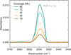 |
Fig. 1 Infrared spectra recorded after the deposition of the five different multilayer H2S ice thicknesses on top of the CsI window. The spectra are centered on the frequency range of the S-H stretching modes of H2S (ν1 and ν3). |
3 Results and discussion
3.1 Binding energies
3.1.1 H2S–H2S
Figure 1 shows the infrared spectra obtained after completing the deposition of the pure H2S ice in the multilayer experiments. The figure focuses on the frequency range of the S-H stretching modes of H2S - its most prominent infrared feature. Five different thicknesses (19, 32, 45, 73, and 90 ML) were used to derive the H2S-H2S binding energy; that is, the binding energy dominated by H2S interactions with other H2S molecules. The TPD curves for each coverage are shown in gray in Fig. 2, measured from the mass-to-charge (m/z) ratio of 34, which corresponds to the molecular ion of H2S and represents its dominant mass signal in electron-impact mass spectrometry at 70 eV ionization energy2.
To fit the TPD curves with the Polanyi-Wigner equation (Eq. (3)), one must first determine the pre-exponential factor νTST of H2S using Eqs. (4), (5), and (6). Since these equations are temperature dependent, we opted to derive νTST at the maximum temperature where the experimental curve is still well described by an exponential behavior. This is to ensure consistency in the data analysis: by choosing the maximum temperature within the exponential range, we ensure that νTST is consistent with the region within which the model is fitted. This temperature is determined on the basis of its adjusted R2 value, a coefficient that measures the proportion of variation in outcomes explained by the model, while adjusting for the number of predictors used. This adjustment is particularly important in this context, as R2 naturally increases with the temperature, even without an improvement in model fit. The maximum temperatures are 79.2, 78.9, 80.5, 80.6, and 81.5 K for the respective coverages of 19, 32, 45, 73, and 90 ML.
As the substrate is warmed up, the morphology of the H2S ice gradually changes toward more ordered configurations, with amorphous-to-crystalline transitions beginning at temperatures as low at ∼30 K, and nearing completion by ∼60 K (Fathe et al. 2006; Mifsud et al. 2024). Although the crystallization process appears to be largely finalized by the onset of desorption (≳70 K), the S-H stretching modes of the H2S ice continue to blueshift as the temperature rises beyond this threshold (see Appendix B and Mifsud et al. 2024), indicating an ongoing reorientation of the ice until its complete desorption. This continued reorientation may contribute to deviations from zeroth-order kinetics near the desorption peak, disrupting the exponential trend. Our approach to the choice of temperature reduces the contribution from these confounding factors to the calculation of the pre-exponential factor.
An alternative, commonly employed approach is to instead use the peak desorption temperature of the TPD curve. In the case of H2S, the temperature differences between the two approaches and their overall impact on the desorption parameters are small: the νTST values derived from the peak desorption T for each coverage (respectively, 82.1, 82.2, 83.0, 84.2, and 84.6 K) deviate by ≲16% from the values derived by our preferred method, resulting in a less than 3% variation in the corresponding binding energies. Uncertainties in the derived νTST values stemming from the absolute error of 2 K in the temperature readout are of ∼1%. We emphasize that the H2S-H2S binding energy derived in this work corresponds to crystalline H2S. However, given that the crystallization of H2S is largely complete by temperatures much lower than its onset of desorption, any thermal desorption of pure H2S from interstellar ices is expected to occur from its crystalline phase.
The νTST values derived for each coverage are used to fit their respective TPD curves with the zeroth-order Polanyi-Wigner equation. Following the above reasoning, the fit is performed for the temperature range where the curve maintains an exponential behavior; that is, until the same maximum temperature for which νTST was calculated. We performed a Monte Carlo analysis using 10 000 independent trials to incorporate and quantify the uncertainties in the ice coverage, absolute substrate temperature, and νTST. In each trial, temperature, coverage, and νTST values were randomly sampled from Gaussian distributions defined by their respective uncertainties. A least-squares fit was then applied to the logarithm of the molecule’s desorption rate versus the inverse of the temperature, optimizing all five experimental curves simultaneously to derive the binding energy (Eb). This transformation, known as an Arrhenius plot, allows the data to be fitted with a straight line, thus mitigating temperaturedependent fitting biases that can arise when applying Monte Carlo sampling to exponential trends.
This analysis yields a mean best-fit H2S-H2S binding energy of Eb = 3159 ± 46 K, shown in the original exponential format by the blue curves in Fig. 2. The log-transformed Arrhenius fits are shown in Appendix C. The uncertainties in Eb are primarily driven by errors in the absolute substrate temperature and in νTST, as the errors in ice coverage and from the fitting are ≲1 K. Given that the uncertainties in νTST due to temperature readout errors are small (∼1%), we adopted the standard deviation from the five experiments (7 1014ML s−1, or 4%) as the νTST error in the fits, which yields uncertainties of ≲5 K in the binding energy. Consequently, most of the uncertainty in Eb are due to the absolute temperature error. Another approach could be to adopt as uncertainties in νTST the full range of values derived for the temperatures within the limits encompassed by the fit. However, this also does not affect the results appreciably: while, in this case, νTST uncertainties correspond to approximately 20%, the resulting mean Eb value remains unchanged, and the error is only increased by 1 K. Additionally, it is also possible to incorporate a temperature-dependent νTST value into the fit, but this approach produces a poorer fit to the data and was thus not preferred (see Appendix D). In some instances, small artifacts are observed at the leading edge, and occasionally symmetrically at the trailing edge of the TPD curves. However, these artifacts have an insignificant impact on the results, with masked fits yielding Eb values that differ by less than 1 K. Table 3 summarizes the recommended desorption parameters derived experimentally for the multilayer H2S ice. The recommended pre-exponential factor is the mean value between all five thicknesses, with its uncertainty corresponding to their standard deviation: νTST = (1.76 ± 0.07)×1016ML s−1.
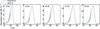 |
Fig. 2 TPD curves of the multilayer H2S ice experiments. The experimental data are shown in gray, and the zeroth-order Polanyi-Wigner models with the dashed blue curve. The shaded blue region indicates the 1σ uncertainty. |
3.1.2 H2S–H2O
Figure 3 shows the TPD curves of the low-coverage H2S ice grown on top of a cASW substrate. In total, six coverages are depicted: 1.6, 1.2, 0.6, 0.5, 0.3, and 0.2 ML (see Appendix A for details on the submonolayer coverage estimation). The two largest thicknesses, 1.6 and 1.2 ML, show nearly overlapping leading edges that culminate in sharp peaks at ∼77 and ∼76 K, respectively - in accordance with the expected dominating zeroth-order desorption behavior. In contrast, the submonolayer coverages display a markedly different profile, with misaligned leading edges and peak desorption temperatures that increase slightly with decreasing coverages (Tpeak ∼79.3, 79.6, 81.1, and 81.3 K for 0.6, 0.5, 0.3, and 0.2 ML). This behavior is consistent with pure first-order desorption, and therefore the 0.6-0.2 ML coverages are used to derive the H2S-H2O binding energy (dominated by H2S interactions with water).
In the case of the submonolayer TPD curves, unlike the multilayer curves, the entire desorption profile is fitted to find Eb . As a result, the peak desorption temperature of the curve is encompassed by the model, and thus we calculated νTST at the peak value for each coverage, which reflects the transition state of the largest parcel of desorbed H2S molecules. Also differently from the multilayer regime, the TPD curves of the submonolayer H2S ice cannot be described by a single binding energy (see Appendix E for an example of an attempted fit). This is a direct consequence of the inhomogeneous nature of the cASW substrate, which generates multiple binding sites that result in a range of H2S-H2O desorption energies. To account for that, we fit a linear combination of first-order Polanyi-Wigner equations (Eq. (3)) to the curves, with statistical weights normalized to the initial ice coverages for each experiment. This allows us to determine the relative population of each binding site. The same approach has been used in the past to derive submonolayer binding energies of hypervolatiles such as N2 and CO, as well as less volatile molecules such as 2-C and 3-C hydrocarbons and methanol, on varying substrates (from water ice to graphite; Doronin et al. 2015; Fayolle et al. 2016; Behmard et al. 2019). Since the pre-exponential factor is calculated using Eqs. (4), (5), and (6), it is treated as a fixed parameter when fitting the curves with a linear combination of Polanyi-Wigner equations. Our sampled desorption energies range from 2000 to 4500 K in steps of 90 K, chosen to balance fit resolution and degeneracies associated with smaller bin sizes. Figure 4 shows the resulting fits to the submonolayer TPD curves and their corresponding binding energy distributions, plotted as fractional coverages as a function of the energy.
The population histograms can be approximated by a normal distribution and are thus fitted by a Gaussian curve to enable a more straightforward interpretation (dashed red line in the right panels in Fig. 4). The mean binding energy and full width at half maximum (FWHM) values for each coverage are listed in Table 3 and can be regarded as representative desorption energies for each ice thickness. The corresponding νTST values used in the fits are also listed, with their uncertainties stemming from the absolute error in the substrate temperature. Among the four coverages, the average binding energy and pre-exponential factor are Eb = 3392±56 K and νTST = (1.7±0.1) 1016 s−1. The uncertainty of Eb encompasses the relative error due to the step size in the binding energy sampling and the standard deviation among the four coverages, while for νTST it is taken solely from its standard deviation.
H2S desorption parameters derived experimentally in this work.
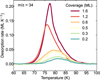 |
Fig. 3 TPD curves of the low-coverage H2S ice experiments deposited on top of a cASW substrate. The transition from zeroth-order to pure first-order sublimation behavior is seen for coverages <1.2 ML. The experimental data are smoothed for clarity. |
3.1.3 Binding energies versus coverage
In Fig. 5, we show a comparison of all H2S binding energies derived in this work as a function of coverage. The multilayer binding energy (Eb ∼ 3159 K) is slightly lower than the submonolayer values, with a difference of 7% w.r.t. the average submonolayer Eb (∼3392 K). This small difference suggests that the H2S-H2S interactions are only moderately weaker than the H2S-H2O counterparts. This is rather expected: both H2S and H2O interact via hydrogen bonding networks - known as one of the strongest intermolecular forces - where hydrogen atoms are covalently bonded to an electronegative atom. Since sulfur is larger than oxygen, it is less electronegative, and therefore the H-bonding networks are weaker for H2S than for H2O. Indeed, the fact that pure first-order desorption could be achieved at coverages of ∼0.6 ML (as evinced by the profile of the TPD curves in Fig. 3; see Sect. 3.1.2) suggests that wetting of the H2S on the cASW surface proceeds relatively uniformly, as opposed to having a tendency to form H2S islands (for comparison, Bergner et al. 2022 found that a dose of 0.04 ML was required to achieve the first-order desorption regime for HCN on cASW). This is in line with a (modest) preference of H2S to interact with H2O.
In the submonolayer regime, the mean H2S-H2O binding energy increases with decreasing ice coverage, in line with other laboratory measurements for various adsorbate-substrate combinations (e.g., Noble et al. 2012; Fayolle et al. 2016; He et al. 2016a; Nguyen et al. 2018; Behmard et al. 2019). This generalized phenomenon can be explained by two effects: 1. lateral interactions influencing the binding energy of the adsorbates, or 2. a preference of the adsorbates to occupy deeper binding sites (caused by their diffusion from shallower sites) - with the most likely explanation being a combination of the two. The weaker H2S-H2S interactions relative to H2S-H2O may manifest as a slight decrease in binding energy caused by lateral H2S interactions compared to isolated H2S adsorbates fully interacting with H2O, in support of explanation 1. Complemen-tarily, the alignment of the trailing edges in the submonolayer experiments suggests that the deeper binding sites are similarly occupied for all explored thicknesses, reinforcing explanation 2.
To the best of our knowledge, this is the first study to experimentally determine binding energies for H2S ice analogs. Nonetheless, estimations based on laboratory data have been proposed in the past. Minissale et al. (2022) recommend a value of Eb = 3426 K for H2S on a cASW substrate based on the peak desorption temperature of H2S and the associated ν obtained using the TST formalism - in good agreement with our measurements. In contrast, the Eb value of 2296±9 K estimated by Penteado et al. (2017), based on the relative peak desorption temperature of H2S with respect to H2O and the binding energy of the latter, differs significantly from our measurements. Computational efforts have also been made to estimate the binding energies of H2S. In general, computed Eb distributions for H2S on water substrates range between 2000 and 3600 K (Wakelam et al. 2017; Das et al. 2018; Ferrero et al. 2020; Piacentino & Öberg 2022), but some studies predict much lower ranges, with upper limits closer to 2000 K (Oba et al. 2018; Bariosco et al. 2024). The experimental values reported here for H2S-H2O (and H2S-H2S) are generally not well reproduced by the computations, often falling within their upper bounds or, in some cases, being entirely under-predicted. This discrepancy is likely due to the limitations in the computational methods for incorporating diffusion as part of their binding energy calculations, which can lead to systematic underestimations by failing to account for the tendency of adsorbates to settle into deeper binding sites prior to sublimating. In an astrophysical context, icy mantles shrouding dust grains are gradually heated by protostellar radiation, in which case adsorbates in shallow sites become free to diffuse throughout the ice and find deeper binding sites before eventually sublimating. The binding energies derived from TPD experiments are therefore expected to better reproduce the conditions in space.
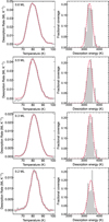 |
Fig. 4 Results of the fits to the submonolayer H2S ice data. Each row corresponds to a different H2S ice thickness: ∼0.6, ∼0.5, ∼0.3, and ∼0.2 ML (from top to bottom). Left panels: TPD curves, with the experimental data in gray and the fits with a linear combination of first-order Polanyi-Wigner equations in red. Right panels: corresponding binding energy distribution: normalized fractional coverages are shown as a functional of the binding energy (gray histogram), superimposed by a Gaussian fit to the distribution (dashed red line). |
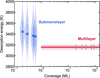 |
Fig. 5 Desorption energies derived experimentally in this work as a function of H2S ice thickness. For the submonolayer regime, the binding energies are represented by blue violin plots, where the square markers indicate the mean binding energies, and the vertical dotted lines show the FWHMs of the Gaussian fits to the binding energy distributions for each coverage. The contour of each violin plot reflects the full range of the sampled binding energy distribution, with its thickness normalized according to the statistical weights (or fractional coverages) of each Eb value. The multilayer binding energy is depicted as a solid red line with its uncertainty shown by the light red shadowed area. The five different ice coverages used to derive the multilayer Eb are shown as gray vertical lines. |
Entrapment efficiencies derived experimentally in this work.
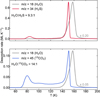 |
Fig. 6 TPD curves of two mixed-ice experiments, H2O:H2S = 9.3:1 (top) and H2O:13CO2 = 14:1 (bottom). The desorption data of H2O, H2S, and 13CO2 are shown in gray (m/z = 18, [H2O]+), red (m/z = 34, [H2S]+), and blue (m/z = 45, [13CO2]+), respectively. Two desorption regimes are seen for H2S: a submonolayer H2S-H2O desorption feature and a molecular volcano desorption peak. For 13CO2, a third regime is observed between its submonolayer and volcano peaks, indicating constant sublimation within that temperature range. |
3.2 Entrapment in H2O
The entrapment behavior of H2S in water-dominated ice was investigated by TPD experiments of H2O:H2S ice mixtures with four different ratios (5.1:1, 7.5:1, 9.3:1, and 17:1, determined from the final infrared spectra measured after deposition) and constant total ice thicknesses (∼40 ML). These mixing conditions are chosen to ensure that H2S is mostly surrounded by H2O molecules while still allowing for measurements with good signal-to-noise ratios, particularly for the more water-dominated cases. Additionally, a control experiment consisting of 13CO2 mixed in H2O ice with a ratio of H2O:13CO2=14:1 was also performed with the goal of testing the potential role of intermolecular interactions on the entrapment efficiencies. H2S and CO2 have similar volatilities, with desorption temperatures typically falling in similar ranges for the same pressure and substrate conditions. However, CO2 is an apolar molecule and its intermolecular interactions with H2O are markedly different from those of H2S. The resulting TPD curves of the H2O:H2S = 9.3:1 experiment, as well as the control H2O:13CO2 = 14:1 experiment, are shown in the upper and lower panels of Fig. 6, respectively.
Two desorption features are observed for H2S ice mixed in H2O: a monolayer desorption peak at ∼84 K, and a molecular volcano feature at ∼150 K. The former is consistent with H2S desorption characterized by the H2S-H2O binding energy (see Appendix F), and includes contributions from H2S adsorbates on the uppermost ice layer, as well as H2S molecules occupying channels within the H2O matrix with access to the surface. The molecular volcano is the strongest desorption peak, and corresponds to H2S being released from the H2O ice matrix as the ice crystallizes and cracks, creating new channels to the surface. In the case of 13CO2, a third desorption regime is observed ranging from ∼90 – 140 K. Following its monolayer desorption feature at ∼80 K, the TPD curve does not return to zero desorption rate, but instead shows a relatively steady desorption of 13CO2 until the molecular volcano feature at ∼150 K - after which it appears to be completely sublimated. This continuous desorption between the two main features might be related to the diffusion of 13CO2 through the H2O ice.
Table 4 lists and Fig. 7 depicts the entrapment efficiencies of H2S and 13CO2 measured from our mixed-ice experiments (see Sect. 2.3 for details on how these are determined). The uncertainties are dominated by experimental variability and are thus taken as 10% of the entrapment efficiency, based on the estimations derived by Simon et al. (2023) with the same experimental setup for H2O:hypervolatile mixtures with ratios 3:1. In comparison, the error due to stochastic instrumental noise amounts to ≲2%. Overall, H2S experiences very efficient entrapment in the H2O-ice matrix, with ∼76 – 85% of the H2S unable to escape to the gas phase until H2O undergoes significant structural changes. This efficient entrapment of H2S has been alluded to in the past by Jiménez-Escobar & Muñoz Caro (2011) based on experiments using H2O:H2S ice mixtures with roughly 10% H2S concentrations. Larger water abundances relative to H2S result in higher entrapment efficiencies, consistent with the behavior observed for many other species mixed in H2O and CO2-dominated ices (Fayolle et al. 2011; Martín-Doménech et al. 2014; Simon et al. 2019, 2023; Kruczkiewicz et al. 2024; Pesciotta et al. 2024). Fayolle et al. (2011) propose two explanations for this phenomenon: (1) there is a reduction in porous channels connected to the surface for higher dilutions of the volatile; and/or (2) higher volatile concentrations increase its diffusion lengths. The two highest dilutions (H2O:H2S ∼9:1 and 17:1) yield analogous efficiencies within their uncertainties, signaling that the trapping capacity of H2S in the H2O ice saturates at ∼85% for our deposition conditions and a total ice thickness of ∼40 ML. Similarly, Pesciotta et al. (2024) recently reported a leveling-off of the entrapment efficiencies of CO in both H2O and CO2 dominated binary ice mixtures starting at concentrations of ≲1:10 volatile:matrix. We emphasize, however, that the CO entrapment saturation measured in their work occurred at significantly lower efficiencies than the saturation point for H2S in H2O measured here (they find 69% and 61% for CO2 and H2O matrices, respectively, in 1:15 CO:matrix ratios and ice thicknesses ≳50 ML).
In comparison to H2S, 13CO2 is significantly less entrapped in the H2O ice, with an efficiency of 52% for a H20:13CO2 ratio of ∼14:1. This stark difference between two similarly volatile molecules might be explained by the nature of their interactions with the water matrix. For 13CO2, the oxygen atoms can serve as hydrogen bond acceptors; however, their very low partial negative charges result in exceptionally weak hydrogen bonds (Zukowski et al. 2017). Interactions between 13CO2 and H2O are thus primarily governed by weaker van der Waals forces. In contrast, the hydrogen bonds between H2S and H2O, while not as strong as H2O-H2O counterparts (Craw & Bacskay 1992), still offer significant energetic stabilization. This is reflected in the mean H2S-H2O binding energy measured here at 3392±56 K, which surpasses the CO2-H2O binding energies measured in the literature by ∼50-60%3. In fact, both Noble et al. (2012) and Edridge et al. (2013) reported CO2-CO2 binding energies to be higher than the mean value for those of CO2-H2O, in clear contrast with the behavior observed here for H2S and water. The difference in the interaction energetics between the two systems (H2O:13CO2 vs. H2O:H2S) may result in H2S diffusing less readily through H2O ice compared to 13CO2, leading to more efficient trapping of H2S. Indeed, the steady desorption of 13CO2 between its monolayer and volcano peaks suggests that it is more mobile than H2S, for which this behavior is minimal. Specifically, this temperature range accounts for ≲5% of the integrated QMS signal in all H2S experiments, and corresponds to only ∼2% in the H2O:H2S = 9.3:1 mixture, compared to ∼21% for 13CO2 in a higher dilution.
In addition to intermolecular interactions, the mass and size of the molecule may also influence its diffusion and entrapment. Based on their molecular masses and kinetic diameters, 13CO2 is ∼30% heavier and ∼9% smaller than H2S ( amu vs.
  amu;
amu;  vs.
vs.  , Matteucci et al. 2006; Ismail et al. 2015). Considering the mass effect alone, the attempt frequency for diffusion of 13CO2 would be smaller than that of H2S, resulting in the former diffusing more slowly (see, e.g., Cuppen et al. 2017) and consequently being more efficiently trapped. The fact that the inverse is observed in our experiments signals that the mass effect is overpowered by other factors favoring the entrapment of H2S. In contrast, the size difference could result in H2S molecules being more efficiently trapped if the mean pore size is smaller than the kinetic diameter of H2S, but larger than that of 13CO2. This size mismatch may create a geometrical limitation, with the pores acting similarly to a net that restricts diffusion. For instance, gas permeance through micro-porous silica membranes (pore size between 3.8 and 5.5 Å) has been shown to decrease steeply with the species’ kinetic diameter, with the permeance of N2 (d ∼ 3.6 Å, similar to H2S; Ismail et al. 2015) being roughly one order of magnitude lower than that of CO2 (De Vos & Verweij 1998). ASW ices are typically found to be microporous (pore width ≤20 Å), with no lower limits estimation for the pore sizes and little to no incidence of mesopores (Mayer & Pletzer 1986; Raut et al. 2007; Cazaux et al. 2015; Carmack et al. 2023). This is particularly true for ices grown through collimated deposition - the technique employed in this work. The possibility of a pore effect therefore cannot be ruled out. Pore effects could also play a role in the constant sublimation regime of CO2, observed between its monolayer and volcano features. The same behavior is seen for 12CO2:H2O ice mixtures in Kruczkiewicz et al. (2024), though they note that this is not observed for other, more volatile species (such as Ar and CO) trapped in H2O-dominated binary ices. Since both Ar and CO have larger kinetic diameters than CO2 (dAr ∼ 3.4 Å and dCO ∼ 3.8 Å; Breck 1973; Matteucci et al. 2006), the fact that they do not display the constant sublimation regime in the experiments by Kruczkiewicz et al. (2024) does not preclude this possibility. Dedicated experimental investigations are necessary to fully constrain the effect of the species’ size and intermolecular interactions to entrapment. Nonetheless, the overall result is that H2S is very efficiently entrapped in H2O ice, more so than other similarly volatile molecules, which has significant implications for its gas versus ice distribution in planet-forming regions.
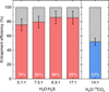 |
Fig. 7 Efficiencies with which H2S (red) and 13CO2 (blue) are trapped in water-rich binary ice mixtures as derived from our experiments (see also Table 4). |
4 Astrophysical implications
The binding energies derived experimentally in this study are used to estimate the locations of the H2S sublimation fronts in the midplane of a representative protoplanetary disk. First, we calculated the desorption temperatures of H2S for its two binding energies (H2S-H2S and H2S-H2O) following the formalism by Hollenbach et al. (2009), in which the desorption temperature is found by equating the flux of molecules adsorbing on the grain surface to the flux of molecules desorbing from it:
![Mathematical equation: T_i\sim(E_{b,i}/k)\left[ \ln{\left( \frac{4N_if_i\nu}{n_iv_i}\right)}\right]^{-1},](/articles/aa/full_html/2025/06/aa54068-25/aa54068-25-eq14.png) (7)
(7)
where Ti is the sublimation temperature of species i, Eb,i is its binding energy, Ni is the number of adsorption sites (assumed to be ∼1015 cm−2), fi is the fraction of such sites occupied by species i, and νi is its vibrational frequency in the surface potential well (i.e., the pre-exponential factor in Eq. (3)). In the denominator, ni is the number density of species i in the gas phase, and νi is its thermal speed. We estimated fi based on the cometary abundance of H2S relative to water, H2S/H2O = 1.10±0.05%, as measured by the Rosetta mission on the coma of comet 67P (Calmonte et al. 2016); and assuming a cometary composition of ∼80% water (e.g., Delsemme 1991). The number density ni is estimated by multiplying the cometary H2S/H2O by the water abundance with respect to H and the number density of hydrogen nuclei in a disk midplane (taken as H2O/H∼10−4; e.g., Drozdovskaya et al. 2015; Boogert et al. 2015; and nH ∼ 1010 cm −3; e.g., Walsh et al. 2014). This yields sublimation temperatures for H2S-H2S and H2S-H2O of ∼64 K and ∼69 K, respectively. For the latter, the mean H2S-H2O binding energy value was used (Eb ∼ 3392 K). We note that the desorption temperatures in the disk model differ from those in the laboratory due to variations in physical conditions between the two environments.
To derive the locations of the sublimation fronts, we assumed a representative disk midplane radial temperature profile:
 (8)
(8)
where r is the radial distance in a.u. This corresponds to the median midplane temperature distribution found for a sample of 24 T-Tauri disks (Andrews & Williams 2007). The resulting sublimation front locations are shown in Fig. 8.
The sublimation fronts for the H2S-H2S and H2S-H2O binding energies occur at ∼6.3 au and ∼5.6 au, respectively. The former corresponds to pure H2S ice desorption, while the latter is relevant for H2S desorbing from a H2O-rich surface. In the case of H2S entrapped in water ice, its sublimation will be delayed to much closer to the water snowline at ∼1.9 au (assuming Eb,H2O ∼ 5600 K, Wakelam et al. 2017; and a typical ν ∼ 1013 s−1). The precise location of this sublimation front will depend on the water crystallization kinetics, but will generally occur at slightly lower temperatures than H2O desorption, placing it just beyond the H2O snowline.
The deuterium fractionation of gaseous H2S observed toward Class 0 protostars suggests that it is formed in ices during early pre-stellar cloud timescales, before the onset of the catastrophic CO freeze-out (Ceccarelli et al. 2014). Most of the water ice is also formed during similarly early timescales, resulting in H2S likely inhabiting a H2O-rich ice environment - the so-called polar ice layer. The sublimation behavior of H2S will therefore be likely dominated by its entrapment within H2O ice, given its high efficiency as measured in this work (∼85% for H2S concentrations of ∼5-10% in H2O). In more representative interstellar scenarios, the bulk H2S concentration in H2O ice is expected to be considerably smaller (≲1% based on observationally constrained H2S ice upper limits), and ice thicknesses larger (≳0.01 μm; Dartois et al. 2018) than our experimental conditions. Like for higher dilutions, entrapment efficiencies have been shown to increase with ice thickness (Fayolle et al. 2011; Simon et al. 2019; Bergner et al. 2022;
Simon et al. 2023; Kruczkiewicz et al. 2024), though this dependence might break down for thicknesses ≳50 ML (Pesciotta et al. 2024). Moreover, the deposition temperatures used in our entrapment experiments generate porous amorphous water ice matrices, whereas more representative cASW might trap volatiles more efficiently than porous counterparts (Kruczkiewicz et al. 2024)4. These three factors (mixing ratios, thicknesses, and water ice morphology) thus point to real H2S entrapment efficiencies being higher than the values measured here, further highlighting the shift in the H2S sublimation front closer to the water snowline. At the same time, differences between the heating rates used in the laboratory and those occurring in astrophysical timescales could result in an overestimation of the measured entrapment efficiencies (Cuppen et al. 2017). Moreover, since sulfur atoms are heavier and less abundant than oxygen, the bulk of the H2S ice has been predicted to form at slightly later timescales (by ∼1.4 AV) than H2O (Goicoechea et al. 2021). This differential formation could result in a concentration gradient for H2S within the polar ice layer, meaning that a fraction of H2S could exists in higher local concentrations than the estimated ≲1%. In any case, the very efficient entrapment of H2S in water, with measured efficiencies of ≳75% for H2S concentrations even as high as 20%, means that even in these scenarios, a significant portion of H2S will remain entrapped in water.
Some ice species, such as CO2 and potentially HCN, exhibit a segregation behavior upon heating, where diffusion leads to the formation of pockets of pure ice instead of a homogeneous mixture (e.g., Öberg et al. 2009; Boogert et al. 2015; Bergner et al. 2022). For H2S, segregation appears to be less energetically favorable than for the archetypal case of CO2. Unlike CO2, the H2S-H2O binding energies exceed that of H2S-H2S, and H2S appears to wet the cASW surface effectively. However, the significantly stronger stabilization among H2O molecules themselves compared to H2S-H2O interactions (Eb (H2O-H2O) 5600 K; Wakelam et al. 2017) may still drive some degree of segregation, as a system with separate water-rich and H2S-rich pockets can be energetically more favorable than a fully mixed one. Similar energetic considerations are required in the kinetic Monte Carlo simulations performed by Öberg et al. (2009) to reproduce the segregation behavior they observed experimentally for CO2:H2O mixed ices5. Consequently, in an astrophysical context, a fraction of H2S within channels with access to the surface might desorb at the sublimation fronts defined by H2S-H2S and H2S-H2O interactions, depending on the extent of segregation.
Nonetheless, the primary sublimation front of H2S is driven by its entrapment. This effectively shifts the H2S sublimation front closer to the protostar by nearly threefold, fully retaining H2S in the ice throughout and beyond the comet-formation zone (>5 au; Mandt et al. 2015), and across the region where other H2O-rich bodies, such as icy asteroids, are formed. Consequently, H2S may be incorporated into planetesimal cores formed beyond the water snowline (∼1.9 au), which in turn may deliver it to terrestrial planets. In fact, Rosetta measurements of the H2S/H2O ratios in the coma of comet 67P remained remarkably constant over several months, strongly suggesting that H2S desorbs from the comet nucleus along with H2O (Calmonte et al. 2016). This supports the hypothesis that H2S is incorporated into cometary cores mixed with H2O, where it remains preserved beyond its sublimation temperature, until water ice desorption.
Additionally, solid-state H2S can react with NH3 to form the ammonium salt NH4+SH− - a likely major carrier of both nitrogen and sulfur in comets (Altwegg et al. 2022; Slavicinska et al. 2025). Upon sublimation, this salt decomposes back into its neutral reactants, releasing H2S (and NH3) into the gas phase. The desorption temperature of the salt is nearly identical to that of water, meaning that the gaseous H2S released from the decomposition of the salt will have a sublimation front similar to that of neutral H2S entrapped in H2O. Distinguishing the contribution from the neutral H2S and the salt to the gas-phase distribution of H2S in disks presents a challenge, but it could be an interesting avenue for future exploration. We emphasize that the neutral H2S component within interstellar ices is likely significant, as the NH4+SH− salt detected by the Rosetta mission is found in the comet’s grains, while the ice predominantly contains H2S in its neutral form (Altwegg et al. 2022).
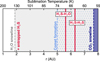 |
Fig. 8 Sublimation front locations for the H2S-H2S and H2S-H2O binding energies estimated for a representative T-Tauri disk midplane. Most of the H2S will remain entrapped in the ice past its sublimation front radii and will only be released to the gas phase close to the water snowline. The CO2 snowline location is also shown for comparison. It was estimated based on the mean binding energy derived by Noble et al. (2012) for (sub)monolayer CO2 ice on a nonporous ASW surface and their adopted pre-exponential factor of 1012 s−1, while assuming ice abundances N(CO2)/N(H2O) 0.28 (median value observed in low-mass young stellar objects; Boogert et al. 2015). |
5 Conclusions
In this work, we provide a comprehensive characterization of the thermal sublimation dynamics of H2S ice. We investigated its binding energies both when dominated by interactions both with other H2S molecules (H2S-H2S) and with H2O molecules (H2S-H2O), as well as the efficiency with which it is entrapped in water-rich ices. This information was used to estimate the different snowline positions of H2S in the midplane of a representative T-Tauri protoplanetary disk. Our main findings are as follows:
We derive Eb = 3159 ± 46 K for the H2S-H2S binding energy, with a mean pre-exponential factor of ν = (1.76 ± 0.07) 1016 ML s−1;
For H2S-H2O, we find four sets of desorption parameters for four different H2S coverages (0.6, 0.5, 0.3, and 0.2 ML). The mean binding energy and pre-exponential factor are Eb = 3392 56 K and ν = (1.7±0.1) 1016 s−1;
Theoretical H2S binding energies generally under-predict the experimental values derived in this work. We propose this mismatch is due to a limitation in the computations in accounting for adsorbate diffusion, causing a preference for H2S occupying deeper surface biding sites. In interstellar and protoplanetary conditions, diffusion plays an important role in a molecule’s sublimation dynamics, and therefore our experimentally derived binding energies are expected to be more representative values;
H2S is very efficiently entrapped in H2O ice, with efficiencies of ∼75-85% for H2O:H2S mixing ratios of 1:∼517 (with more diluted cases resulting in more efficient entrapment). In comparison, 13CO2 is much less efficiently entrapped, with an efficiency of ∼52% for a H2O:13CO2 ratio of 1:14. We suggest this might be due to the hydrogen bonding networks between H2S and H2O, which are stronger intermolecular interactions than the induced dipoles between 13CO2 and H2O. Pore effects could also play a role in entrapping H2S more efficiently than 13CO2;
Our measured H2S-H2S and H2S-H2O binding energies yield H2S sublimation temperatures of ∼64 K and ∼69 K, respectively. This corresponds to a radial distance of ∼6.3 au and ∼5.6 au in the midplane of a representative T-Tauri disk;
The vast majority of H2S will remain entrapped in the ice until water crystallizes at radii close to the H2O snowline, shifting its sublimation front inward by nearly a factor of 3. As a result, most of the H2S will remain in ices throughout the region where water-rich icy planetesimals form.
Acknowledgements
J.C.S. acknowledges support from the Danish National Research Foundation through the Center of Excellence “InterCat” (Grant agreement no.: DNRF150) and the Leiden University Fund/Fonds Van Trigt (Grant reference no.: W232310-1-055). K.I.Ö. acknowledges an award from the Simons Foundation (#321183FY19).
Appendix A Submonolayer coverage estimation
The submonolayer H2S coverages were estimated based on a QMS-to-column density scaling factor, f , derived from the multilayer H2S experiments. Figure A.1 shows the correlation between the H2S ice column density obtained from the integrated absorbance of its S-H stretching feature (see Eq. (2)) and the integrated signal of the H2S desorption feature as measured by the QMS for m/z = 34.
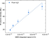 |
Fig. A.1 H2S column densities derived from the integrated absorbance of its S-H stretching modes at 15 K for each multilayer ice thickness as a function of its corresponding integrated desorption feature as measured by the QMS. The dashed blue line shows the linear fit to the points from which the QMS-to-column density scaling factor was derived. |
A linear fit to the plot gives the conversion factor f = (3.2 ± 0.4) 1026 A−1 K−1. In the low coverage experiments, where H2S was deposited on top of cASW, the H2S ices with approximately 1.6 ML and 1.2 ML (determined from their infrared absorbance bands) produced S-H stretching features detectable above our instrumental noise. By comparing the measured and predicted H2S coverages in these experiments, we estimate that the submonolayer coverages might be under-predicted by up to a factor of 2 using our scaling method. However, this discrepancy does not impact our analysis, as the higher coverages (by a factor of 2) yield binding energy distributions with mean Eb values differing by less than 2 K from those derived for the predicted coverages - well within their FWHMs.
Appendix B Pure H2S ice infrared features versus temperature
Figure B.1 shows the infrared spectra recorded during the TPD experiment of a multilayer H2S ice with an initial coverage of 73 ML. The splitting between its symmetric (ν1) and antisymmetric (ν3) S-H stretching modes signals that ice crystallization starts to occur at temperatures as low as 30 K. By 65 K, the transition to phase III crystalline H2S is nearly complete. However, from 65 K up to the point of complete desorption, a continuous blueshift in the S-H stretching features is observed, suggesting ongoing structural reorganization within the ice. While higher-energy crystalline phases of H2S exist (phase II transitioning at 100 K and phase I transitioning at 125 K; see Fathe et al. 2006 and references therein), these transitions are observed under ambient pressure and occur above the sublimation temperature of H2S in UHV conditions. They are therefore not relevant to our experiments.
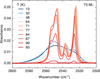 |
Fig. B.1 Infrared spectra taken during the TPD experiment of the 73 ML H2S ice, centered on the frequency range of its S-H stretching modes. For clarity, only a subset of spectra collected at the relevant temperatures are shown. |
Appendix C Arrhenius plots
Figure C.1 shows the Arrhenius plots of the TPD experiments of all multilayer H2S ice coverages. The desorption rate data (gray) for all five thicknesses was fit simultaneously following a MonteCarlo sampling approach with 10 000 trials. The mean best-fit model corresponds to an H2S-H2S binding energy of Eb = 3159 ± 46 K (dashed blue lines).
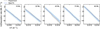 |
Fig. C.1 Arrhenius plots of the multilayer H2S TPD curves used to derive the H2S-H2S binding energy. The experimental data are shown in gray, and the linear fits to the plots, performed simultaneously for the five ice thicknesses, with the dashed blue lines. The shaded blue region indicates the 1σ uncertainty. The fit is performed for the temperature range where the original curve follows an exponential trend (see Sect. 3.1.1). |
Appendix D Multilayer H2S ice fits with a temperature-dependent νTST
Figures D.1 and D.2 show the fits to the log-transformed multilayer TPD curves of H2S with a temperature-dependent νTST. The former presents the data as the original TPD profile, while the latter shows the corresponding Arrhenius plots. This approach yields Eb = 3141 ± 49 K (dashed blue lines).
Appendix E Submonolayer fit with a single energy component
Figure E.1 illustrates an attempted fit of the 0.2 ML H2S ice using the Polanyi-Wigner equation (Eq. (3)) with a single temperature component. The fit fails to capture the experimental data, highlighting the presence of a distribution of binding energies caused by the inherent inhomogeneity of the cASW substrate.
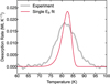 |
Fig. E.1 TPD curve of the 0.2 ML H2S ice experiment deposited on top of a cASW substrate. The experimental data are show in gray, and the attempted fit to the data with a first-order Polanyi-Wigner curve with only one temperature component in red. |
Appendix F QMS-TPD results for mixed H2O:H2S ices
Figure F.1 presents the QMS data collected for m/z = 34 during the TPD experiments with mixed H2O:H2S ices. In all cases, the first desorption feature (panel a) corresponds to monolayer desorption characterized by the H2S-H2O binding energies. This is evinced by the peak desorption temperatures, which increase with decreasing coverages, and by the desorption profiles consistent with first-order desorption kinetics for all mixing ratios. The second desorption feature (panel b) corresponds to the molecular volcano.
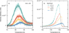 |
Fig. F.1 TPD data measured by the QMS for m/z = 34 in the experiments with mixed H2O:H2S ices. Panel a: Monolayer desorption of H2S molecules with access to the surface. Panel b: Molecular volcano feature due to H2S entrapped in the H2O ice matrix. |
References
- Accolla, M., Congiu, E., Manicò, G., et al. 2013, MNRAS, 429, 3200 [NASA ADS] [CrossRef] [Google Scholar]
- Aikawa, Y., van Zadelhoff, G. J., van Dishoeck, E. F., & Herbst, E. 2002, A&A, 386, 622 [NASA ADS] [CrossRef] [EDP Sciences] [Google Scholar]
- Altwegg, K., Balsiger, H., Berthelier, J. J., et al. 2017, Philos. Trans. Roy. Soc. Lond. Ser. A, 375, 20160253 [Google Scholar]
- Altwegg, K., Combi, M., Fuselier, S. A., et al. 2022, MNRAS, 516, 3900 [NASA ADS] [CrossRef] [Google Scholar]
- Andrews, S. M., & Williams, J. P. 2007, ApJ, 659, 705 [NASA ADS] [CrossRef] [Google Scholar]
- Bar-Nun, A., Kleinfeld, I., & Kochavi, E. 1988, Phys. Rev. B, 38, 7749 [Google Scholar]
- Bariosco, V., Pantaleone, S., Ceccarelli, C., et al. 2024, MNRAS, 531, 1371 [NASA ADS] [CrossRef] [Google Scholar]
- Behmard, A., Fayolle, E. C., Graninger, D. M., et al. 2019, ApJ, 875, 73 [Google Scholar]
- Bergin, E. A., & Langer, W. D. 1997, ApJ, 486, 316 [Google Scholar]
- Bergner, J. B., Rajappan, M., & Öberg, K. I. 2022, ApJ, 933, 206 [Google Scholar]
- Biver, N., Bockelée-Morvan, D., Moreno, R., et al. 2015, Sci. Adv., 1, 1500863 [NASA ADS] [CrossRef] [Google Scholar]
- Bockelée-Morvan, D., Lis, D. C., Wink, J. E., et al. 2000, A&A, 353, 1101 [Google Scholar]
- Boogert, A. C. A., Gerakines, P. A., & Whittet, D. C. B. 2015, ARA&A, 53, 541 [Google Scholar]
- Bossa, J. B., Isokoski, K., de Valois, M. S., & Linnartz, H. 2012, A&A, 545, A82 [NASA ADS] [CrossRef] [EDP Sciences] [Google Scholar]
- Bouilloud, M., Fray, N., Bénilan, Y., et al. 2015, MNRAS, 451, 2145 [Google Scholar]
- Breck, D. 1973, Zeolite Molecular Sieves: Structure, Chemistry, and Use (Wiley) [Google Scholar]
- Burke, D. J., & Brown, W. A. 2010, Phys. Chem. Chem. Phys. (Incorp. Faraday Trans.), 12, 5947 [Google Scholar]
- Calmonte, U., Altwegg, K., Balsiger, H., et al. 2016, MNRAS, 462, S253 [NASA ADS] [CrossRef] [Google Scholar]
- Carmack, R. A., Tribbett, P. D., & Loeffler, M. J. 2023, ApJ, 942, 1 [NASA ADS] [CrossRef] [Google Scholar]
- Cazaux, S., Bossa, J. B., Linnartz, H., & Tielens, A. G. G. M. 2015, A&A, 573, A16 [NASA ADS] [CrossRef] [EDP Sciences] [Google Scholar]
- Ceccarelli, C., Caselli, P., Bockelée-Morvan, D., et al. 2014, in Protostars and Planets VI, eds. H. Beuther, R. S. Klessen, C. P. Dullemond, & T. Henning, 859 [Google Scholar]
- Chen, Y. J., Juang, K. J., Nuevo, M., et al. 2015, ApJ, 798, 80 [Google Scholar]
- Craw, J. S., & Bacskay, G. B. 1992, J. Chem. Soc. Faraday Trans., 88, 2315 [Google Scholar]
- Cuppen, H. M., Walsh, C., Lamberts, T., et al. 2017, Space Sci. Rev., 212, 1 [Google Scholar]
- Cuppen, H. M., Linnartz, H., & Ioppolo, S. 2024, ARA&A, 62, 243 [Google Scholar]
- Dartois, E., Chabot, M., Id Barkach, T., et al. 2018, A&A, 618, A173 [NASA ADS] [CrossRef] [EDP Sciences] [Google Scholar]
- Das, A., Sil, M., Gorai, P., Chakrabarti, S. K., & Loison, J. C. 2018, ApJS, 237, 9 [NASA ADS] [CrossRef] [Google Scholar]
- De Vos, R. M., & Verweij, H. 1998, Science, 279, 1710 [Google Scholar]
- Delsemme, A. H. 1991, in Astrophysics and Space Science Library, 167, IAU Colloq. 116: Comets in the post-Halley era, eds. J. Newburn, R. L., M. Neugebauer, & J. Rahe, 377 [Google Scholar]
- Doronin, M., Bertin, M., Michaut, X., Philippe, L., & Fillion, J. H. 2015, J. Chem. Phys., 143, 084703 [NASA ADS] [CrossRef] [Google Scholar]
- Drozdovskaya, M. N., Walsh, C., Visser, R., Harsono, D., & van Dishoeck, E. F. 2015, MNRAS, 451, 3836 [NASA ADS] [CrossRef] [Google Scholar]
- Drozdovskaya, M. N., van Dishoeck, E. F., Jørgensen, J. K., et al. 2018, MNRAS, 476, 4949 [Google Scholar]
- Drozdovskaya, M. N., van Dishoeck, E. F., Rubin, M., Jørgensen, J. K., & Altwegg, K. 2019, MNRAS, 490, 50 [Google Scholar]
- Druard, C., & Wakelam, V. 2012, MNRAS, 426, 354 [NASA ADS] [CrossRef] [Google Scholar]
- Dunning Jr, T. H. 1989, J. Chem. Phys., 90, 1007 [NASA ADS] [CrossRef] [Google Scholar]
- Edridge, J. L., Freimann, K., Burke, D. J., & Brown, W. A. 2013, Philos. Trans. Roy. Soc. Lond. Ser. A, 371, 20110578 [Google Scholar]
- Esplugues, G., Viti, S., Goicoechea, J., & Cernicharo, J. 2014, A&A, 567, A95 [NASA ADS] [CrossRef] [EDP Sciences] [Google Scholar]
- Fathe, K., Holt, J. S., Oxley, S. P., & Pursell, C. J. 2006, J. Phys. Chem. A, 110, 10793 [Google Scholar]
- Fayolle, E. C., Öberg, K. I., Cuppen, H. M., Visser, R., & Linnartz, H. 2011, A&A, 529, A74 [NASA ADS] [CrossRef] [EDP Sciences] [Google Scholar]
- Fayolle, E. C., Balfe, J., Loomis, R., et al. 2016, ApJ, 816, L28 [Google Scholar]
- Ferrante, R. F., Moore, M. H., Spiliotis, M. M., & Hudson, R. L. 2008, ApJ, 684, 1210 [NASA ADS] [CrossRef] [Google Scholar]
- Ferrero, S., Zamirri, L., Ceccarelli, C., et al. 2020, ApJ, 904, 11 [NASA ADS] [CrossRef] [Google Scholar]
- Frisch, M. J., Trucks, G. W., Schlegel, H. B., et al. 2016, Gaussian∼16 Revision C.01 (Wallingford, CT: Gaussian Inc.) [Google Scholar]
- Garozzo, M., Fulvio, D., Kanuchova, Z., Palumbo, M. E., & Strazzulla, G. 2010, A&A, 509, A67 [NASA ADS] [CrossRef] [EDP Sciences] [Google Scholar]
- Garrod, R. T., Wakelam, V., & Herbst, E. 2007, A&A, 467, 1103 [NASA ADS] [CrossRef] [EDP Sciences] [Google Scholar]
- Gerakines, P. A., Schutte, W. A., Greenberg, J. M., & van Dishoeck, E. F. 1995, A&A, 296, 810 [NASA ADS] [Google Scholar]
- Goicoechea, J. R., Aguado, A., Cuadrado, S., et al. 2021, A&A, 647, A10 [EDP Sciences] [Google Scholar]
- Hatchell, J., Thompson, M. A., Millar, T. J., & MacDonald, G. H. 1998, A&A, 338, 713 [Google Scholar]
- He, J., Acharyya, K., & Vidali, G. 2016a, ApJ, 825, 89 [Google Scholar]
- He, J., Acharyya, K., & Vidali, G. 2016b, ApJ, 823, 56 [Google Scholar]
- Henning, T., & Semenov, D. 2013, Chem. Rev., 113, 9016 [Google Scholar]
- Herbst, E., & van Dishoeck, E. F. 2009, ARA&A, 47, 427 [NASA ADS] [CrossRef] [Google Scholar]
- Hollenbach, D., Kaufman, M. J., Bergin, E. A., & Melnick, G. J. 2009, ApJ, 690, 1497 [NASA ADS] [CrossRef] [Google Scholar]
- Hudson, R. L., & Gerakines, P. A. 2018, ApJ, 867, 138 [CrossRef] [Google Scholar]
- Ismail, A. F., Khulbe, K. C., & Matsuura, T. 2015, Switz. Springer, 10, 973 [Google Scholar]
- Jiménez-Escobar, A., & Muñoz Caro, G. M. 2011, A&A, 536, A91 [Google Scholar]
- Jiménez-Escobar, A., Muñoz Caro, G. M., & Chen, Y. J. 2014, MNRAS, 443, 343 [Google Scholar]
- Kruczkiewicz, F., Dulieu, F., Ivlev, A. V., et al. 2024, A&A, 686, A236 [NASA ADS] [CrossRef] [EDP Sciences] [Google Scholar]
- Laas, J. C., & Caselli, P. 2019, A&A, 624, A108 [NASA ADS] [CrossRef] [EDP Sciences] [Google Scholar]
- Le Roy, L., Altwegg, K., Balsiger, H., et al. 2015, A&A, 583, A1 [NASA ADS] [CrossRef] [EDP Sciences] [Google Scholar]
- Linnartz, H., Ioppolo, S., & Fedoseev, G. 2015, Int. Rev. Phys. Chem., 34, 205 [Google Scholar]
- Loeffler, M. J., Hudson, R. L., Chanover, N. J., & Simon, A. A. 2015, Icarus, 258, 181 [NASA ADS] [CrossRef] [Google Scholar]
- Madhusudhan, N. 2019, ARA&A, 57, 617 [NASA ADS] [CrossRef] [Google Scholar]
- Mandt, K. E., Mousis, O., Marty, B., et al. 2015, Space Sci. Rev., 197, 297 [Google Scholar]
- Martín-Doménech, R., Muñoz Caro, G. M., Bueno, J., & Goesmann, F. 2014, A&A, 564, A8 [NASA ADS] [CrossRef] [EDP Sciences] [Google Scholar]
- Matteucci, S., Yampolskii, Y., Freeman, B. D., & Pinnau, I. 2006, Mater. Sci. Membr. Gas Vapor Sep., 1 [Google Scholar]
- Mayer, E., & Pletzer, R. 1986, Nature, 319, 298 [NASA ADS] [CrossRef] [Google Scholar]
- McClure, M. K., Rocha, W. R. M., Pontoppidan, K. M., et al. 2023, Nat. Astron., 7, 431 [NASA ADS] [CrossRef] [Google Scholar]
- Mifsud, D. V., Herczku, P., Ramachandran, R., et al. 2024, Spectroch. Acta A: Mol. Spectrosc., 319, 124567 [Google Scholar]
- Minh, Y. C., Irvine, W. M., & Ziurys, L. M. 1989, ApJ, 345, L63 [NASA ADS] [CrossRef] [Google Scholar]
- Minh, Y. C., Ziurys, L. M., Irvine, W. M., & McGonagle, D. 1990, ApJ, 360, 136 [NASA ADS] [CrossRef] [Google Scholar]
- Minissale, M., Aikawa, Y., Bergin, E., et al. 2022, ACS Earth Space Chem., 6, 597 [NASA ADS] [CrossRef] [Google Scholar]
- Moore, M. H., Hudson, R. L., & Carlson, R. W. 2007, Icarus, 189, 409 [CrossRef] [Google Scholar]
- Mumma, M. J., & Charnley, S. B. 2011, ARA&A, 49, 471 [NASA ADS] [CrossRef] [Google Scholar]
- Neufeld, D. A., Godard, B., Gerin, M., et al. 2015, A&A, 577, A49 [NASA ADS] [CrossRef] [EDP Sciences] [Google Scholar]
- Nguyen, T., Baouche, S., Congiu, E., et al. 2018, A&A, 619, A111 [NASA ADS] [CrossRef] [EDP Sciences] [Google Scholar]
- Noble, J. A., Congiu, E., Dulieu, F., & Fraser, H. J. 2012, MNRAS, 421, 768 [NASA ADS] [Google Scholar]
- Oba, Y., Tomaru, T., Lamberts, T., Kouchi, A., & Watanabe, N. 2018, Nat. Astron., 2, 228 [NASA ADS] [CrossRef] [Google Scholar]
- Öberg, K. I. 2016, Chem. Rev., 116, 9631 [Google Scholar]
- Öberg, K. I., Fayolle, E. C., Cuppen, H. M., van Dishoeck, E. F., & Linnartz, H. 2009, A&A, 505, 183 [NASA ADS] [CrossRef] [EDP Sciences] [Google Scholar]
- Öberg, K. I., Murray-Clay, R., & Bergin, E. A. 2011, ApJ, 743, L16 [Google Scholar]
- Öberg, K. I., Facchini, S., & Anderson, D. E. 2023, ARA&A, 61, 287 [CrossRef] [Google Scholar]
- Olson, K. R., & Straub, K. D. 2016, Physiology, 31, 60 [Google Scholar]
- Penteado, E. M., Walsh, C., & Cuppen, H. M. 2017, ApJ, 844, 71 [Google Scholar]
- Pesciotta, C., Simon, A., Rajappan, M., & Öberg, K. I. 2024, ApJ, 973, 166 [Google Scholar]
- Phuong, N. T., Chapillon, E., Majumdar, L., et al. 2018, A&A, 616, L5 [NASA ADS] [CrossRef] [EDP Sciences] [Google Scholar]
- Piacentino, E. L., & Öberg, K. I. 2022, ApJ, 939, 93 [NASA ADS] [CrossRef] [Google Scholar]
- Polman, J., Waters, L. B. F. M., Min, M., Miguel, Y., & Khorshid, N. 2023, A&A, 670, A161 [NASA ADS] [CrossRef] [EDP Sciences] [Google Scholar]
- Raut, U., Famá, M., Teolis, B. D., & Baragiola, R. A. 2007, J. Chem. Phys., 127, 204713 [NASA ADS] [CrossRef] [Google Scholar]
- Rivière-Marichalar, P., Fuente, A., Esplugues, G., et al. 2022, A&A, 665, A61 [NASA ADS] [CrossRef] [EDP Sciences] [Google Scholar]
- Rivière-Marichalar, P., Fuente, A., Le Gal, R., et al. 2021, A&A, 652, A46 [NASA ADS] [CrossRef] [EDP Sciences] [Google Scholar]
- Rubin, M., Altwegg, K., Balsiger, H., et al. 2018, Sci. Adv., 4, eaar6297 [NASA ADS] [CrossRef] [Google Scholar]
- Santos, J. C., Enrique-Romero, J., Lamberts, T., Linnartz, H., & Chuang, K.-J. 2024a, ACS Earth Space Chem., 8, 1646 [NASA ADS] [CrossRef] [Google Scholar]
- Santos, J. C., Linnartz, H., & Chuang, K. J. 2024b, A&A, 690, A24 [NASA ADS] [CrossRef] [EDP Sciences] [Google Scholar]
- Simon, A., Öberg, K. I., Rajappan, M., & Maksiutenko, P. 2019, ApJ, 883, 21 [NASA ADS] [CrossRef] [Google Scholar]
- Simon, A., Rajappan, M., & Öberg, K. I. 2023, ApJ, 955, 5 [NASA ADS] [CrossRef] [Google Scholar]
- Slavicinska, K., Boogert, A. C. A., Tychoniec, ., et al. 2025, A&A, 693, A146 [NASA ADS] [CrossRef] [EDP Sciences] [Google Scholar]
- Smith, R. G. 1991, MNRAS, 249, 172 [NASA ADS] [CrossRef] [Google Scholar]
- Smith, R. S., Huang, C., Wong, E. K. L., & Kay, B. D. 1997, Phys. Rev. Lett., 79, 909 [NASA ADS] [CrossRef] [Google Scholar]
- Tait, S. L., Dohnálek, Z., Campbell, C. T., & Kay, B. D. 2005, J. Chem. Phys., 122, 164708 [NASA ADS] [CrossRef] [Google Scholar]
- Thaddeus, P., Kutner, M. L., Penzias, A. A., Wilson, R. W., & Jefferts, K. B. 1972, ApJ, 176, L73 [NASA ADS] [CrossRef] [Google Scholar]
- Tsai, S.-M., Lee, E. K. H., Powell, D., et al. 2023, Nature, 617, 483 [CrossRef] [Google Scholar]
- van Dishoeck, E. F. 2014, Faraday Discuss., 168, 9 [NASA ADS] [CrossRef] [Google Scholar]
- van Dishoeck, E. F., Blake, G. A., Jansen, D. J., & Groesbeck, T. D. 1995, ApJ, 447, 760 [Google Scholar]
- Vastel, C., Phillips, T. G., Ceccarelli, C., & Pearson, J. 2003, ApJ, 593, L97 [Google Scholar]
- Vidal, T. H. G., & Wakelam, V. 2018, MNRAS, 474, 5575 [Google Scholar]
- Vidal, T. H. G., Loison, J.-C., Jaziri, A. Y., et al. 2017, MNRAS, 469, 435 [Google Scholar]
- Viti, S., Collings, M. P., Dever, J. W., McCoustra, M. R. S., & Williams, D. A. 2004, MNRAS, 354, 1141 [NASA ADS] [CrossRef] [Google Scholar]
- Vitorino, J., Loison, J. -C., Wakelam, V., Congiu, E., Dulieu, F. 2024, MNRAS, 533, 52 [NASA ADS] [CrossRef] [Google Scholar]
- Wakelam, V., Castets, A., Ceccarelli, C., et al. 2004, A&A, 413, 609 [NASA ADS] [CrossRef] [EDP Sciences] [Google Scholar]
- Wakelam, V., Loison, J. C., Mereau, R., & Ruaud, M. 2017, Mol. Astrophys., 6, 22 [NASA ADS] [CrossRef] [Google Scholar]
- Walsh, C., Millar, T. J., Nomura, H., et al. 2014, A&A, 563, A33 [NASA ADS] [CrossRef] [EDP Sciences] [Google Scholar]
- Yarnall, Y. Y., & Hudson, R. L. 2022, ApJ, 931, L4 [CrossRef] [Google Scholar]
- Zhao, Y., & Truhlar, D. G. 2008, Theor. Chem. Acc., 120, 215 [CrossRef] [Google Scholar]
- Zhou, Q., Simon, A., Öberg, K. I., & Rajappan, M. 2024, ApJ, 972, 189 [Google Scholar]
- Zukowski, S. R., Mitev, P. D., Hermansson, K., & Ben-Amotz, D. 2017, J. Phys. Chem. Lett., 8, 2971 [Google Scholar]
Surface Processing Apparatus for Chemical Experimentation-Kinetics of Ice Transformation in Thermal ENvironments.
Noble et al. (2012) and Edridge et al. (2013) measured the mean monolayer CO2 binding energy on ASW to be 2247 K and 2100 K, respectively. The former was measured on a nonporous ASW substrate, while the latter was measured on porous ASW.
Previously, Burke & Brown (2010) suggested that more compact ASW should result in lower entrapment efficiencies due to a reduction in available trapping sites. This interpretation was based on earlier experiments by Bar-Nun et al. (1988), which observed lower entrapment efficiencies of hypervolatiles in binary mixtures with water ice as the deposition temperature increased. However, this decline is more likely dominated by the reduced surface residence time of hypervolatiles at higher deposition temperatures (Zhou et al. 2024), rather than due to the water ice morphology. Recently, Kruczkiewicz et al. (2024) deposited cASW ices at 10 K using well-collimated beams, and found that trapping capacities were actually higher for the compact ice structure.
Öberg et al. (2009) find that segregation in CO2:H2O ice mixtures is not precluded by CO2-CO2 binding energies being lower than those of CO2-H2O. Rather, it might occur when a CO2 molecule from a water-dominated environment is swapped with a H2O molecule from a CO2-dominated environment. This process only requires that 0.5×Eb (H2O-H2O)+0.5×Eb(CO2-CO2) is greater than Eb(H2O-CO2).
All Tables
All Figures
|
Fig. 1 Infrared spectra recorded after the deposition of the five different multilayer H2S ice thicknesses on top of the CsI window. The spectra are centered on the frequency range of the S-H stretching modes of H2S (ν1 and ν3). |
| In the text | |
|
Fig. 2 TPD curves of the multilayer H2S ice experiments. The experimental data are shown in gray, and the zeroth-order Polanyi-Wigner models with the dashed blue curve. The shaded blue region indicates the 1σ uncertainty. |
| In the text | |
|
Fig. 3 TPD curves of the low-coverage H2S ice experiments deposited on top of a cASW substrate. The transition from zeroth-order to pure first-order sublimation behavior is seen for coverages <1.2 ML. The experimental data are smoothed for clarity. |
| In the text | |
|
Fig. 4 Results of the fits to the submonolayer H2S ice data. Each row corresponds to a different H2S ice thickness: ∼0.6, ∼0.5, ∼0.3, and ∼0.2 ML (from top to bottom). Left panels: TPD curves, with the experimental data in gray and the fits with a linear combination of first-order Polanyi-Wigner equations in red. Right panels: corresponding binding energy distribution: normalized fractional coverages are shown as a functional of the binding energy (gray histogram), superimposed by a Gaussian fit to the distribution (dashed red line). |
| In the text | |
|
Fig. 5 Desorption energies derived experimentally in this work as a function of H2S ice thickness. For the submonolayer regime, the binding energies are represented by blue violin plots, where the square markers indicate the mean binding energies, and the vertical dotted lines show the FWHMs of the Gaussian fits to the binding energy distributions for each coverage. The contour of each violin plot reflects the full range of the sampled binding energy distribution, with its thickness normalized according to the statistical weights (or fractional coverages) of each Eb value. The multilayer binding energy is depicted as a solid red line with its uncertainty shown by the light red shadowed area. The five different ice coverages used to derive the multilayer Eb are shown as gray vertical lines. |
| In the text | |
|
Fig. 6 TPD curves of two mixed-ice experiments, H2O:H2S = 9.3:1 (top) and H2O:13CO2 = 14:1 (bottom). The desorption data of H2O, H2S, and 13CO2 are shown in gray (m/z = 18, [H2O]+), red (m/z = 34, [H2S]+), and blue (m/z = 45, [13CO2]+), respectively. Two desorption regimes are seen for H2S: a submonolayer H2S-H2O desorption feature and a molecular volcano desorption peak. For 13CO2, a third regime is observed between its submonolayer and volcano peaks, indicating constant sublimation within that temperature range. |
| In the text | |
|
Fig. 7 Efficiencies with which H2S (red) and 13CO2 (blue) are trapped in water-rich binary ice mixtures as derived from our experiments (see also Table 4). |
| In the text | |
|
Fig. 8 Sublimation front locations for the H2S-H2S and H2S-H2O binding energies estimated for a representative T-Tauri disk midplane. Most of the H2S will remain entrapped in the ice past its sublimation front radii and will only be released to the gas phase close to the water snowline. The CO2 snowline location is also shown for comparison. It was estimated based on the mean binding energy derived by Noble et al. (2012) for (sub)monolayer CO2 ice on a nonporous ASW surface and their adopted pre-exponential factor of 1012 s−1, while assuming ice abundances N(CO2)/N(H2O) 0.28 (median value observed in low-mass young stellar objects; Boogert et al. 2015). |
| In the text | |
|
Fig. A.1 H2S column densities derived from the integrated absorbance of its S-H stretching modes at 15 K for each multilayer ice thickness as a function of its corresponding integrated desorption feature as measured by the QMS. The dashed blue line shows the linear fit to the points from which the QMS-to-column density scaling factor was derived. |
| In the text | |
|
Fig. B.1 Infrared spectra taken during the TPD experiment of the 73 ML H2S ice, centered on the frequency range of its S-H stretching modes. For clarity, only a subset of spectra collected at the relevant temperatures are shown. |
| In the text | |
|
Fig. C.1 Arrhenius plots of the multilayer H2S TPD curves used to derive the H2S-H2S binding energy. The experimental data are shown in gray, and the linear fits to the plots, performed simultaneously for the five ice thicknesses, with the dashed blue lines. The shaded blue region indicates the 1σ uncertainty. The fit is performed for the temperature range where the original curve follows an exponential trend (see Sect. 3.1.1). |
| In the text | |
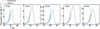 |
Fig. D.1 Same as Fig. 2 but with fits performed using a temperature-dependent νTST. |
| In the text | |
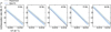 |
Fig. D.2 Same as Fig. C.1 but with fits performed using a temperature-dependent νTST. |
| In the text | |
|
Fig. E.1 TPD curve of the 0.2 ML H2S ice experiment deposited on top of a cASW substrate. The experimental data are show in gray, and the attempted fit to the data with a first-order Polanyi-Wigner curve with only one temperature component in red. |
| In the text | |
|
Fig. F.1 TPD data measured by the QMS for m/z = 34 in the experiments with mixed H2O:H2S ices. Panel a: Monolayer desorption of H2S molecules with access to the surface. Panel b: Molecular volcano feature due to H2S entrapped in the H2O ice matrix. |
| In the text | |
Current usage metrics show cumulative count of Article Views (full-text article views including HTML views, PDF and ePub downloads, according to the available data) and Abstracts Views on Vision4Press platform.
Data correspond to usage on the plateform after 2015. The current usage metrics is available 48-96 hours after online publication and is updated daily on week days.
Initial download of the metrics may take a while.