| Issue |
A&A
Volume 698, June 2025
|
|
|---|---|---|
| Article Number | A126 | |
| Number of page(s) | 12 | |
| Section | Planets, planetary systems, and small bodies | |
| DOI | https://doi.org/10.1051/0004-6361/202453454 | |
| Published online | 12 June 2025 | |
OGLE-2015-BLG-1609Lb: A sub-Jovian planet orbiting a low-mass stellar or brown dwarf host
1
Astronomical Observatory, University of Warsaw,
Al. Ujazdowskie 4,
00-478
Warszawa,
Poland
2
Department of Earth and Space Science, Graduate School of Science, Osaka University,Toyonaka,
Osaka
560-0043,
Japan
3
Zentrum für Astronomie der Universität Heidelberg, Astronomisches Rechen-Institut,
Mönchhofstr. 12–14,
69120
Heidelberg,
Germany
4
Department of Particle Physics and Astrophysics, Weizmann Institute of Science,
Rehovot
76100,
Israel
5
Department of Physics, University of Warwick,
Coventry
CV4 7AL,
UK
6
Villanova University, Department of Astrophysics and Planetary Sciences,
800 Lancaster Ave.,
Villanova,
PA
19085,
USA
7
Institute for Space-Earth Environmental Research, Nagoya University,
Nagoya
464-8601,
Japan
8
Code 667, NASA Goddard Space Flight Center,
Greenbelt,
MD
20771,
USA
9
Department of Astronomy, University of Maryland,
College Park,
MD
20742,
USA
10
Institute of Natural and Mathematical Sciences, Massey University,
Auckland
0745,
New Zealand
11
Department of Earth and Planetary Science, Graduate School of Science, The University of Tokyo,
7-3-1 Hongo, Bunkyo-ku,
Tokyo
113-0033,
Japan
12
Instituto de Astrofísica de Canarias, Vía Lacteá s/n,
38205
La Laguna, Tenerife,
Spain
13
Institute of Astronomy, Graduate School of Science, The University of Tokyo,
2-21-1 Osawa, Mitaka,
Tokyo
181-0015,
Japan
14
Oak Ridge Associated Universities,
Oak Ridge,
TN
37830,
USA
15
Institute of Space and Astronautical Science, Japan Aerospace Exploration Agency,
Kanagawa
252-5210,
Japan
16
Sorbonne Université, CNRS, UMR 7095, Institut d’Astrophysique de Paris,
98 bis bd Arago,
75014
Paris,
France
17
Department of Physics, University of Auckland,
Private Bag 92019,
Auckland,
New Zealand
18
University of Canterbury Mt. John Observatory,
P.O. Box 56,
Lake Tekapo
8770,
New Zealand
19
Las Cumbres Observatory Global Telescope Network,
6740 Cortona Drive, suite 102,
Goleta,
CA
93117,
USA
20
IPAC,
Mail Code 100-22, Caltech, 1200 E. California Blvd.,
Pasadena,
CA
91125,
USA
21
Università degli Studi di Salerno, Dipartimento di Fisica “E.R. Caianiello”, via Ponte Don Melillo,
84085
Fisciano (SA),
Italy
22
Istituto Nazionale di Fisica Nucleare, Sezione di Napoli, Via Cintia,
Napoli
80126,
Italy
23
SUPA, School of Physics & Astronomy, University of St Andrews,
North Haugh,
St Andrews
KY16 9SS,
UK
24
Millennium Institute of Astrophysics MAS,
Nuncio Monsenor Sotero Sanz 100, Of. 104, Providencia,
Santiago,
Chile
25
Instituto de Astrofísica, Facultad de Física, Pontificia Universidad Católica de Chile,
Av. Vicuña Mackenna 4860,
7820436
Macul, Santiago,
Chile
26
Institute for Astronomy, University of Edinburgh, Royal Observatory,
Edinburgh
EH9 3HJ,
UK
27
Astrophysics Research Institute, Liverpool John Moores University,
Liverpool
CH41 1LD,
UK
28
South African Astronomical Observatory,
PO Box 9,
Observatory
7935,
South Africa
29
Centre for ExoLife Sciences, Niels Bohr Institute, University of Copenhagen,
Jagtvej 155,
2200
Copenhagen,
Denmark
30
Centro de Astronomía (CITEVA), Universidad de Antofagasta, Avda. U. de Antofagasta
02800,
Antofagasta,
Chile
31
Instituto de Astrofísica e Ciências do Espaço, Universidade de Coimbra,
3040-004
Coimbra,
Portugal
32
Centre for Electronic Imaging, Department of Physical Sciences, The Open University,
Milton Keynes
MK7 6AA,
UK
33
Astrophysics Group, Keele University,
Staffordshire
ST5 5BG,
UK
34
Universität Hamburg, Faculty of Mathematics, Informatics and Natural Sciences, Department of Earth Sciences, Meteorological Institute,
Bundesstraße 55,
20146
Hamburg,
Germany
35
Centro de Astroingeniería, Facultad de Física, Pontificia Universidad Católica de Chile,
Av. Vicuña Mackenna 4860, Macul
7820436,
Santiago,
Chile
36
University of Southern Denmark, Department of Physics, Chemistry and Pharmacy, SDU-Galaxy,
Campusvej 55,
5230
Odense M,
Denmark
37
Jodrell Bank, School of Physics and Astronomy, University of Manchester,
Oxford Road,
Manchester
M13 9PL,
UK
38
Dipartimento di Fisica, Università di Roma Tor Vergata,
Via della Ricerca Scientifica 1,
00133
Roma,
Italy
39
Max Planck Institute for Astronomy,
Königstuhl 17,
69117,
Heidelberg,
Germany
40
INAF – Turin Astrophysical Observatory,
Via Osservatorio 20,
I-10025,
Pino Torinese,
Italy
41
Universidad Catolica de la Santisima,
Concepcion,
Chile
42
Department of Physics, Sharif University of Technology,
PO Box 11155-9161,
Tehran,
Iran
★ Corresponding author.
Received:
16
December
2024
Accepted:
2
April
2025
Abstract
We present a comprehensive analysis of the planetary microlensing event OGLE-2015-BLG-1609. The planetary anomaly was detected by two survey telescopes, OGLE and MOA. Both surveys collected enough data over the planetary anomaly to enable an unambiguous planet detection. Such survey detections of planetary anomalies are needed to build a robust sample of planets, which could improve studies on the microlensing planetary occurrence rate by reducing biases and statistical uncertainties. In this work we examined different methods for modeling microlensing events using individual datasets. In particular, we incorporated a Galactic model prior to better constrain the poorly defined microlensing parallax. Ultimately, we fitted a comprehensive model to all available data, identifying three potential topologies, with two showing comparably high Bayesian evidence. Our analysis indicates that the host of the planet is either a brown dwarf, with a probability of 34%, or a low-mass stellar object (M dwarf), with a probability of 66%. The topology that provides the best fit to the data results in an extraordinary low host mass, Mh = 0.025+0.050-0.012M⊙, accompanied by an Earth-mass planet with Mc = 1.9+3.9-1.0M⊕.
Key words: gravitation / gravitational lensing: micro / planets and satellites: detection
© The Authors 2025
 Open Access article, published by EDP Sciences, under the terms of the Creative Commons Attribution License (https://creativecommons.org/licenses/by/4.0), which permits unrestricted use, distribution, and reproduction in any medium, provided the original work is properly cited.
This article is published in open access under the Subscribe to Open model. This email address is being protected from spambots. You need JavaScript enabled to view it. to support open access publication.
1 Introduction
More than three decades have passed since Mao & Paczynski (1991) first suggested that extrasolar planets could be detected in microlensing events. During this time, over 230 planets1 have been discovered using this method. This number may seem small compared to discoveries made by other major planet-detection techniques, but the strength of microlensing lies in its unique sensitivity to low-mass and distant planets. Instead of analyzing the light of the planet’s host star, microlensing uses the light of an unrelated background star to probe the foreground planetary system. This makes the technique sensitive to, for example, planets at and beyond the snow line of their host stars, as well as to those located at distances from the Galactic center that are currently inaccessible by any other method (Tsapras 2018).
Another advantage of microlensing is its usefulness in demographic studies2. In microlensing, planetary occurrence rates are typically derived as a function of mass ratios (q) and projected separations in Einstein ring radius units (s), calculated using a set of events and the detection efficiency of the survey that detected them (Mróz & Poleski 2024). However, these analyses are affected by uncertainties and biases that require significant effort to disentangle (e.g., Gould et al. 2010; Udalski et al. 2018). These factors are inherent to the sample of analyzed microlensing events, starting with observational data collected by numerous surveys using various instruments and under differing conditions. Furthermore, variations in data reduction and selection processes, along with subjective human factors such as publication bias (Yang et al. 2020), contribute to these uncertainties. Collecting a sample of events detected from homogeneous data gathered by a single instrument greatly minimizes these issues.
We present the discovery of the planetary microlensing event OGLE-2015-BLG-1609. The planetary signal in this event was identified solely through a single survey, making it well-suited for the statistical analysis of microlensing planets. The analysis turned out to be more complex than typical, due to low-level systematic trends in the photometry. We find that there are three different topologies that could explain the light curve of the event; two of them have very similar Bayesian evidence, and hence, we were not able to distinguish between them. We estimated the mass of the planet host, which overlaps with masses of both stars and brown dwarfs.
One of the most detailed studies on the planetary occurrence rate in microlensing events was done by the Microlensing Observations in Astrophysics (MOA) collaboration, using their 2007–2012 sample (Suzuki et al. 2016). This sample comprised 1474 events, including 23 planetary events. Suzuki et al. (2016) find that the planetary occurrence rate follows a broken power law of q. However, due to the lack of events in the sample with q < 10−4.5, which is close to the break in the power law (qbr), fitting qbr led to a high uncertainty for all the parameters. Therefore, the authors fixed this value to qbr = 1.7 × 10⁻⁴ and concluded that beyond the snow line, most planets should have Neptune-like masses. Later, known planets with q < 10−4 were analyzed by Udalski et al. (2018). Combining planets detected using both survey and follow-up data forced authors to apply an alternative inference method (the V/Vmax method; Schmidt 1968). Udalski et al. (2018) confirmed the break in the mass ratio power law but at higher masses, qbr = 2 × 10⁻⁴. The break was further analyzed by Jung et al. (2019) using a sample of 15 planets with q < 3 × 10⁻⁴ and assuming that planet-detection sensitivity as a function of q can be approximated by a simple power law. Their results suggest that the break is at a much smaller mass ratio (qbr ≈ 0.55 × 10⁻⁴) and the slope of the distribution at lower mass ratios is much steeper compared to the findings by Suzuki et al. (2016).
Significant efforts are currently being undertaken, using the Korea Microlensing Telescope Network’s (KMTNet) semiautomated algorithm Anomalyfinder (Zang et al. 2021), to build a large, uniformly selected sample of planetary events. So far, the algorithm has identified about 100 planets in KMTNet’s observations from the years 2016–2019 (Zang et al. 2021; Hwang et al. 2022; Wang et al. 2022; Gould et al. 2022; Zang et al. 2022; Jung et al. 2022; Zang et al. 2023; Jung et al. 2023; Shin et al. 2023; Ryu et al. 2024; Shin et al. 2024), including a few with q < 0.5 × 10⁻⁴. A future statistical analysis of this sample will significantly improve constraints on planetary occurrence rates, in particular in the low-mass regime. The projected separation and the mass ratio are not the only parameters that can be derived from microlensing events. By measuring the so-called secondary effects in the light curve, it is possible to obtain absolute masses, the distance to the system, and the projected separation in physical units. For this purpose, a pair of finite-source and microlensing parallax effects is typically used. Despite the fact that both of these effects are measured only in ~20% of planetary events, some initiatives were taken to measure how the distribution of the planets depends on the host mass and Galactocentric distance (Mh, R). The hypothesis of an equal abundance of planets in the bulge and the disk was tested by Penny et al. (2016) using a sample of 21 systems. However, the small sample of the parallax measurements, hindered by systematic uncertainties, prevented them from reaching a definitive conclusion. Additionally, some nearby planets (< 2 kpc) in the sample have now been shown, through analysis of high-angular-resolution images, to be at larger distances than originally reported, for example, MOA-2007-BLG-192 (Terry et al. 2024). Using a slightly larger sample (28 planets), Koshimoto et al. (2021b) derived the planetary occurrence rate as a function of both host mass (Mh) and Galactocentric distance (R), ![Mathematical equation: $\[P_{\text {host }} \propto M_{\mathrm{h}}^{m} R^{r}\]$](/articles/aa/full_html/2025/06/aa53454-24/aa53454-24-eq3.png) , by comparing the observed distribution of lens-source relative proper motion (μrel) to Galactic model predictions for a given Einstein radius crossing time (tE). Their results suggest that the probability of hosting a planet increases with the Galactocentric distance, but this dependence is not statistically significant, with r = 0.2 ± 0.4. The uncertainties in the exponents of Mh and R were reduced by Nunota et al. (2024) by utilizing model distributions of both μrel and tE and dividing systems into two subsamples, with mass ratios below and above q = 10−3. Their analyses indicate that beyond the snow line, massive planets are more likely to be around more massive stars, while the frequency of low-mass planets does not depend on the mass of the host.
, by comparing the observed distribution of lens-source relative proper motion (μrel) to Galactic model predictions for a given Einstein radius crossing time (tE). Their results suggest that the probability of hosting a planet increases with the Galactocentric distance, but this dependence is not statistically significant, with r = 0.2 ± 0.4. The uncertainties in the exponents of Mh and R were reduced by Nunota et al. (2024) by utilizing model distributions of both μrel and tE and dividing systems into two subsamples, with mass ratios below and above q = 10−3. Their analyses indicate that beyond the snow line, massive planets are more likely to be around more massive stars, while the frequency of low-mass planets does not depend on the mass of the host.
The planetary event analyzed here will be included in the statistical studies of MOA or Optical Gravitational Lensing Experiment (OGLE) survey planets. Such studies can shed more light on the detailed aspects of the planetary occurrence rate.
This paper is organized as follows: in Sect. 2 we describe the observational data and their preliminary analysis. In Sect. 3, we detail the model fitting to the OGLE observations alone. In Sect. 4, we present the final results of modeling using all available datasets and the process of estimating the physical parameters of the system. Finally, we summarize our results in Sect. 5.
2 Observational data
2.1 Collection
The microlensing event OGLE-2015-BLG-1609 was first detected by OGLE on 2015 June 16, heliocentric Julian date (HJD) ~2457219. The detection was made by the Early Warning System (EWS3; Udalski 2003) through the analysis of data collected by the 1.3-m Warsaw Telescope, equipped with the 1.4 deg2 field of view mosaic CCD camera at the Las Campanas Observatory in Chile (Udalski et al. 2015). The event was located at (RA, Dec)2000 = (18:03:17.71, -26:54:25.6) in equatorial coordinates, or (l, b) = (![Mathematical equation: $\[3^\circ_\cdot72,-2^\circ_\cdot34\]$](/articles/aa/full_html/2025/06/aa53454-24/aa53454-24-eq4.png) ) in Galactic coordinates, which is inside the BLG511 field of the OGLE-IV survey. This field was one of the OGLE high-cadence Galactic Bulge fields, observed four times per night on average. OGLE images were primarily taken in the I band, with occasional observations in the V band conducted approximately once every few days. The reduction of the OGLE data was done using a variant of difference image analysis (DIA; Crotts & Tomaney 1996; Alard & Lupton 1998) optimized by Wozniak (2000) and Udalski et al. (2008).
) in Galactic coordinates, which is inside the BLG511 field of the OGLE-IV survey. This field was one of the OGLE high-cadence Galactic Bulge fields, observed four times per night on average. OGLE images were primarily taken in the I band, with occasional observations in the V band conducted approximately once every few days. The reduction of the OGLE data was done using a variant of difference image analysis (DIA; Crotts & Tomaney 1996; Alard & Lupton 1998) optimized by Wozniak (2000) and Udalski et al. (2008).
The event was also observed by MOA’s 1.8 m telescope at Mt. John University Observatory in New Zealand. It was independently alerted on 2015 June 30, HJD ~ 2457233, as MOA-2015-BLG-412 on the MOA alerts web page4. MOA observations were primarily done in the custom wide MOA-Red filter, approximately equal to the sum of R− and I− band filters. MOA data reductions were performed using a variation of DIA presented by Bond et al. (2001). Additionally, MOA observed in the V band, but these few observations were excluded in this analysis due to large error bars.
On 2015 September 3, HJD ~ 2457269, the light curve visibly deviated from the standard Paczynski (1986) model, indicating the presence of a planetary anomaly. This triggered follow-up observations on three 1 m Las Cumbres Observatory (LCO) telescopes located at the South African Astronomical Observatory, operated by the RoboNet collaboration (Tsapras et al. 2009), and on the 1.54 m Danish Telescope at La Silla Observatory, Chile, operated by the Microlensing Network for the Detection of Small Terrestrial Exoplanets5 (MiNDSTEp) collaboration (Dominik et al. 2010). RoboNet data reductions were performed using a modified DIA algorithm (DANDIA; Bramich 2008). Observations on the Danish Telescope were collected using a high frame-rate electron-multiplying CCD (Skottfelt et al. 2015) and were reduced using a variation of the DANDIA algorithm optimized for this instrument. The light curve of the event is plotted in Fig. 1, with a closer view of the planetary anomaly provided in Fig. 2. Some data were collected using other telescopes but due to poor coverage of the event, large error bars, or the lack of reliable reductions, we excluded them from this analysis.
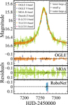 |
Fig. 1 Light curves of the microlensing event OGLE-2015-BLG-1609 with three microlensing model topologies for positive values of the impact parameter, u0. The difference between the topologies is visible only during the planetary anomaly (HJD ~ 2457270; see Fig. 2). The photometry comes from the OGLE, MOA, RoboNet, and MiNDSTEp projects. |
2.2 Preliminary analysis
In the initial analysis of OGLE-2015-BLG-1609 based solely on the OGLE survey data, we faced several challenges. In models that include the microlensing parallax effect, we obtained well-constrained but astrophysically unlikely values for the northern component of the parallax vector (πE,N), which should be close to zero according to the Galactic models (e.g., Lam et al. 2020; Koshimoto et al. 2021a). Additionally, at the end of the event and before the annual break in the visibility of the Galactic bulge, a trend at HJD 2457300–2457335 was noticed in the residuals from the best fit. We tried to solve these issues by including additional effects in microlensing models. First considered was the binary source effect (2L2S). In this model, the brightening at the end of the event was caused by the presence of a second star in the source system. Inclusion of this effect improved χ2 of the fit, but did not change the value of πE,N. Since only half of the second source brightening was covered by data points, we conclude that this trend is more likely an end-of-the-season effect than an astrophysical one, and we rule out the binary source explanation.
We also considered additional changes in the geometry of the event caused by either the orbital motion of the lenses or the orbital motion of the source (the xallarap effect). In the case of lens orbital motion, we did not achieve reasonable constraints on the effect’s parameters, nor did we improve the χ2 statistics of the fits. This could be attributed to the lack of distinctive features in the light curve, such as caustic structures, that can serve as time references (An & Gould 2001). Similarly, in models with the xallarap effect, there was no improvement in the χ2 statistics. Additionally, the resulting values of the orbital period of the source aligned with spurious periods of low-level amplitude recurring in the OGLE photometric data, as found in previous studies (Mróz et al. 2023). These periods are associated with the structure of the data itself. For this reason, we do not consider the results of xallarap models to be trustworthy. Including lens orbital motion or xallarap effects in the models did not change the values of πE,N. The overestimation of the parallax vector may be caused by other unassociated photometric variability. To address the potential trends in our data we incorporated Gaussian processes into modeling of the event. This approach has been successful in modeling the variability of the microlensing source, demonstrated in the analysis of the event OGLE-2017-BLG-1186 (Li et al. 2019). Unfortunately, it led to an increase in the πE,N value with even smaller uncertainties. Simultaneous modeling both the variability of the source star and the parallax effect requires careful selection of the baseline time range. A long baseline is needed to reliably constrain the long-term stellar variability. However, extending the baseline much beyond the duration of the microlensing event can adversely affect parallax vector measurements by introducing uncorrelated trends.
Finally, to ensure the absence of long-term observational trends in the light curve of the event, we analyzed observations of the nearby stars in the OGLE database. We selected 16 constant stars in the OGLE database around 30″ from the source star, with similar brightness and color. We arranged their observations in week-long bins, then calculated the average between all the chosen stars. The resulting trend did not exceed the average magnitude uncertainty of the analyzed data and thus could not affect the microlensing modeling.
After trying all the approaches described above, we decided to include the data collected by the MOA group in our analysis. Models fitted to the MOA data alone and to the combined MOA and OGLE datasets provided more typical results for the πE,N value, which was consistent with zero within the 2σ limit. This led us to make a step back and take a closer look at the reductions of the OGLE images. In the DIA reduction method, photometric measurements are obtained by subtracting a reference image from the acquired images. The reference images are created by averaging a selected dozen or so images taken under the best seeing conditions. For the initial OGLE reductions, reference images were selected from those taken at the start of the 2010 season. Three years after the event, in 2018, the OGLE team prepared new reference images. Since they were closer in time to the analyzed event, we used them to re-extract the photometry. We fitted the model with parallax effect to this new OGLE dataset. This time we obtained a distribution of πE,N that was consistent with zero within the 2σ limit and, therefore, in a good agreement with the Galactic model. The photometry extracted using DIA can be affected at a low level by the proper motion of the source star. Hence, changes in the position of the source star can influence microlensing parallax measurements. We present in Table 1 proper motion measurements from the Gaia DR3 (Gaia Collaboration 2023) and the internal OGLE time-series astrometry, which has been matched to the Gaia DR3 reference frame. We note that the uncertainties in the OGLE measurements are purely statistical and likely underestimated. The value of the renormalized unit weight error (RUWE > 1.5; Table 1) for the Gaia DR3 asymmetric solution indicates that the parallax measurements from Gaia DR3 cannot be attributed to either the lens or the source in the event (Wyrzykowski et al. 2023).
In all cases, the binary-lens models fitted to individual datasets from both the “old” and “new” OGLE reductions, as well as MOA observations, have significantly lower-χ2 statistics compared to the single-lens models fitted to the same datasets. This enables the inclusion of this event in the planetary occurrence rate studies of both surveys. The comparison is shown in the Table 2. In the subsequent investigation, we used new OGLE reductions only.
Proper motion of the source in the OGLE-2015-BLG-1609 event.
2.3 Data preparation and photometric uncertainties
We performed the color calibration of the OGLE I – and V-and measurements, so that magnitudes reported in this work are in the standard I (Cousins) and V (Johnson) pass-bands. To clean datasets, we excluded all observations with error bars larger than five times the median of the error bars of nearby points. Additionally, using one of the early models of the event, we removed 3σ outliers from the fitted light curve.
Photometric pipelines sometimes struggle with estimating the impact of systematics in the data; uncertainties in the raw measurements are often underestimated and have broader tails than a Gaussian. To renormalize photometric error bars, we scaled them using the formula for the i-th data point (Yee et al. 2012):
![Mathematical equation: $\[\sigma_{\mathrm{new}, i}=\sqrt{\left(k \sigma_i\right)^2+e_{\min }^2},\]$](/articles/aa/full_html/2025/06/aa53454-24/aa53454-24-eq5.png) (1)
(1)
where σi is an initial error bar, k and emin are re-normalization coefficients. Since we used new reference images for OGLE data reductions, the values of k and emin from the empirical model for this dataset reported by Skowron et al. (2016) could be inaccurate. For the sake of coherent treatment of each dataset, we regarded k and emin for each dataset as additional parameters of the model and sampled with Markov chain Monte Carlo (MCMC). We assumed that error bars should be Gaussian in flux space, and used the modified likelihood function in the form of
![Mathematical equation: $\[\begin{aligned}\ln~ \mathcal{L} & =-\frac{1}{2} \sum_{i=1}^N\left[\left(\frac{f_i-f_{\text {mod}, i}}{\sigma_{\text {new}, i}}\right)^2+~\ln \left(2 \pi \sigma_{\text {new}, i}^2\right)\right] \\& =-\frac{1}{2}\left[\chi^2+\sum_{i=1}^N ~\ln \left(2 \pi \sigma_{\text {new}, i}^2\right)\right],\end{aligned}\]$](/articles/aa/full_html/2025/06/aa53454-24/aa53454-24-eq6.png) (2)
(2)
where fi − fmod,i represents the difference between the measured and modeled flux values at the i-th observation. All the modeling presented in this work was initially done using this approach. Then, the error bars scaling parameters were fixed to the values from the models with the lowest χ2, and the modeling was repeated.
Comparison of χ2 statistics.
3 Single instrument data modeling: OGLE
As the planetary anomaly is well sampled in the OGLE observations alone, initially we focused on just this dataset in our analysis. The observed brightening in the OGLE-2015-BLG1609 light curve, except for the anomaly, can be described well by the classical Paczynski (1986) model. In this single-lens point-source model (1L1S), microlensing magnification is described by
![Mathematical equation: $\[A(u)=\frac{u^2+2}{u \sqrt{u^2+4}},\]$](/articles/aa/full_html/2025/06/aa53454-24/aa53454-24-eq7.png) (3)
(3)
where u(t) denotes the projected separation between the source and the lens at a given time, scaled to the angular Einstein radius (θE). This separation is related to the impact parameter of the lens-source approach (u0) and the time of closest approach (t0) through the relation
![Mathematical equation: $\[u(t)=\sqrt{u_0^2+\tau(t)^2} \quad \text { and } \quad \tau(t)=\frac{t-t_0}{t_{\mathrm{E}}}.\]$](/articles/aa/full_html/2025/06/aa53454-24/aa53454-24-eq8.png) (4)
(4)
Taking into account that not all the measured light is magnified, the flux change as a function of time is given by
![Mathematical equation: $\[f(t)=f_{\mathrm{S}} A+f_{\mathrm{B}},\]$](/articles/aa/full_html/2025/06/aa53454-24/aa53454-24-eq9.png) (5)
(5)
where fS and fB are the fluxes of the source and blended objects, respectively. As the starting point of our analysis, we excluded data points collected during the anomaly (HJD 2457267–2457273) and fitted the Paczyński curve to the remaining observations. The 1L1S parameters (tE, t0, and u0) were used as initial values for further modeling. Next, we considered the binarylens single-source (2L1S) model, which is outlined in Sect. 3.1. We extended this model by including the microlensing parallax effect (Sect. 3.2). Moreover, due to unreliable parameter constraints, we also imposed priors on πE based on a Galactic model, which is described in Sect. 3.3.
All the microlensing modeling in this work was done using the MulensModel Python-code (Poleski & Yee 2019), with the affine invariant MCMC ensemble sampler (Goodman & Weare 2010) implemented in the emcee code (Foreman-Mackey et al. 2013). The number of chains and steps for each MCMC modeling run was adjusted to achieve the convergence. All runs with fixed error bars scaling parameters had a mean acceptance fraction between 0.287 and 0.458, the number of steps is at least 34 times longer than the mean autocorrelation time, and no thinning was applied (for definitions, see Foreman-Mackey et al. 2013).
3.1 Binary-lens model
The planetary anomaly in the light curve led us to consider a binary-lens model with finite-source effect (2L1S). This model requires extending the number of parameters from three in Paczyński’s model to seven. Those additional parameters are typically: s – the projected separation between the primary lens and the companion, q – the ratio of the companion’s mass to the primary lens mass, α – the angle between the source trajectory and the binary axis, and the parameter of the finite source effect: ρ – the radius of the source in the Einstein radius units. In our modeling, we used this parametrization. Other alternative parametrization were not suitable, as most of them are connected to features of the light curve involving caustic crossings, which are absent in the analyzed event.
To find all the degenerate solutions, we conducted a grid search in the log s − log q parameters space. We used fixed values of s evenly spaced between −0.15 < log s < 0.35 and q spaced between −4.5 < log q < −2, and optimized with MCMC method values of other parameters (tE, t0 u0, ρ, and α). As the absence of a visible caustic crossing results in poor constraints on α, we split our modeling into two steps. First, we spread uniformly starting values of α and ran EMCEE with 300 walkers. After confirming that all models across log s − log q grid gave consistent constraints on α, we repeated modeling with a narrowed starting range of α. We show the resulting χ2 map in Fig. 3.
We identified three possible topologies, depending on the source trajectory with respect to the position of the caustic (Gaudi & Gould 1997). The inner-large q topology is in the case in which the trajectory crosses between the central and the planetary caustic; outer-large q, in which the trajectory passes behind the planetary caustic with respect to the central caustic; and an intermediate case, small q, in which the trajectory passes through the planetary caustic, possible only in the case of a small mass ratio between the lenses (Fig. 4). The small q topology should suffer the same “inner-outer” degeneracy as in the case of large q topologies. However, the absence of a sudden and strong brightening typical of caustic-crossing in the observed light curve implies that if the trajectory of the source indeed crosses the planetary caustic, the projected size of the source must be comparable to the size of the caustic. Thus, the inner-outer degeneracy in the small q topology does not result in two separated groups of solutions due to the finite-source effect. Finally, we fitted each of the three topologies separately, with all parameters freed. For s and q the starting values were taken from the lowest-χ2 models and these parameters were constrained to the ranges marked in Fig. 3.
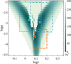 |
Fig. 3 Δχ2 map in (log s, log q) parameter space for OGLE-2016-BLG-1609. We named the three visible topologies according to the projected separation: inner-large q (labeled A and delineated by the dashed blue line), small q (B, dot-dashed orange line), and outer-large q (C, dotted green line). Crosses mark the lowest-χ2 models for each topology, and boxes represent the s and q limits used in modeling. |
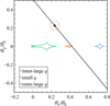 |
Fig. 4 Source trajectory and caustics of OGLE-2015-BLG-1609 for different binary lens topologies: inner-large q (blue line), small q (orange line), and outer-large q (green line). The central caustics of the small q and inner-large q models at the point (θx/θE, θy/θE) = (0, 0) are approximately point-like. For clarity, we plot only the small q topology trajectory, as the other trajectories differed only slightly. The orange circle represents the size of the source in the case of the small q topology. |
3.2 2L1S model with the parallax effect
To obtain an estimate of the absolute values of the lens masses, additional effects in the light curve have to be considered. Typically, the most prominent effect is the microlensing parallax. It is a deviation from the straight trajectory of the source in the lens plane caused by the Earth’s orbital motion. This effect can be used as a source of information on the relative movement of the source and the lens. We introduced this effect into our models by adding north and east components of the microlensing parallax vector, πE,N and πE,E, as parameters.
Because the parallax effect breaks the symmetry between positive u0 and negative u0 topologies, we additionally split our models between positive and negative u0 values. The introduction of the parallax effect lowered the χ2 statistic of our models. However, for all considered topologies, the obtained absolute values of the north component of the parallax vector were exceptionally large (πE,N = ![Mathematical equation: $\[-1.85_{-0.45}^{+0.61}\]$](/articles/aa/full_html/2025/06/aa53454-24/aa53454-24-eq10.png) , for the inner-large q topology with positive u0), as shown in Fig. 5. These results contrast with the predictions from the Galactic models, which suggest |πE,N| ⪅ 0.5 (see Fig. 6). Additionally, fitting the models separately to OGLE and MOA datasets resulted in distinctly different πE posteriors (Fig. 5).
, for the inner-large q topology with positive u0), as shown in Fig. 5. These results contrast with the predictions from the Galactic models, which suggest |πE,N| ⪅ 0.5 (see Fig. 6). Additionally, fitting the models separately to OGLE and MOA datasets resulted in distinctly different πE posteriors (Fig. 5).
3.3 Galactic prior
For the new OGLE reductions, we repeated additional analyses conducted for the initial reductions (including the addition of the xallarap effect, the 2L2S models, and the Gaussian-process-correlated noise modeling). However, none of these approaches resulted in reliable improvements in χ2 or in the values of πE For these reasons, we incorporated priors on πE,N and πE,E in our modeling, based on the Galactic model from Koshimoto et al. (2021a) and Koshimoto & Ranc (2022). We estimated the input event parameters for the Galactic model by summing the distributions of all three 2L1S u0+ topologies (inner-large q, small q, outer-large q), and considered the 3σ posterior scatter of the selected parameters, as summarized in Table 3. With those settings, we simulated a sample of 5 × 10⁷ microlensing events with the genulens code (Koshimoto & Ranc 2022). As priors for the Bayesian inference we used the resulting samples of πE,N and πE,E, which were broadened in order to obtain proper sampling of wings of the posterior distribution. We achieved that by averaging simulated samples with normal distributions with μ = 0.05, σ = 0.30 and μ = 0.03, σ = 0.28, respectively. These values of μ and σ were determined by fitting Gaussian functions to the simulated πE,N and πE,E distributions, with the resulting σ values scaled by a factor of 4. Figure 6 presents the priors alongside the original probability distribution functions of the simulated events. The parameters resulting from the modeling are summarized in Table 4, and the obtained distributions of πE values are included in Fig. 5.
3.4 Binary-source model
The anomaly in the OGLE-2015-BLG-1609 light curve lacks characteristic features associated with caustic crossing that could unambiguously determine its planetary nature. Therefore, this brightening can alternatively be explained by the presence of a secondary star in the source system. In the single-lens binary-source (1L2S) model, effective magnification is given by the normalized sum of the magnifications of the two sources:
![Mathematical equation: $\[A=\frac{A_1 f_{\mathrm{S}, 1}+A_2 f_{\mathrm{S}, 2}}{f_{\mathrm{S}, 1}+f_{\mathrm{S}, 2}},\]$](/articles/aa/full_html/2025/06/aa53454-24/aa53454-24-eq11.png) (6)
(6)
where Ai denotes the lensing magnification of each source star with a flux Fi. Ai is given analogously to Eqs. (3) and (4), under the assumption that the transverse speed of the two sources with respect to the lens is the same. Thus, the inclusion of a secondary source doubles the parameters associated with the source and its trajectory (i.e., u0,1, u0,2, t0,1, t0,2, ρ1, ρ2, fS,1, and fS,2). The 1L2S model suffers from an analogous degeneracy for positive and negative values of the impact parameter, similar to the single-source interpretation, resulting in two degenerate solutions: (u0,1+, u0,2+) and (u0,1+, u0,2−), where the signs indicate positive and negative values. The inclusion of the parallax effect additionally breaks the symmetry, leading to four possible solutions: (u0,1+, u0,2+),(u0,1+, u0,2−), (u0,1+, u0,2+), and (u0,1+, u0,2−).
Initially, as for binary-lens model, we fitted the binary-source model without accounting of parallax effect separately to the MOA and OGLE data. This model fitted both datasets fairly well, having a significantly lower-χ2 statistic than the 1L1S model but still slightly higher than the binary-lens interpretation, in the case of the OGLE data, as presented in Table 2. The MOA dataset is missing observations from two nights at the beginning of the anomaly, leading to weaker constraints on the 1L2S model and a slightly lower-χ2 statistic compared to the 2L1S model. Nevertheless, in all cases, the recovered parameters of the models were difficult to justify astrophysically. The timescales of magnification for the two sources are drastically different. For the primary source, it corresponds to the timescale of the entire event, while for the secondary source, it is the timescale of the anomaly. Since tE is common for both sources, reproducing this difference requires the secondary source to pass significantly closer to the lens than the primary source (|u0,2| ≈ 0.007) and to be substantially dimmer than the primary source. The absence of a sharp brightening during the anomaly in the light curve further suggests a strong influence of finite-source effects, placing tight constraints on the diameter of the secondary source. In conclusion, in the 1L2S model, the secondary source must be dimmer but not necessarily smaller than the primary source. For the (u0,1+, u0,2−) model fitted to the OGLE dataset, ratio of the angular diameters of the sources ρ1/ρ2 = ![Mathematical equation: $\[1.14_{-0.79}^{+0.85}\]$](/articles/aa/full_html/2025/06/aa53454-24/aa53454-24-eq12.png) and their brightens in the I-band fS,1,I/ fS,2,I =
and their brightens in the I-band fS,1,I/ fS,2,I = ![Mathematical equation: $\[195_{-19}^{+17}\]$](/articles/aa/full_html/2025/06/aa53454-24/aa53454-24-eq13.png) , for MOA dataset these values are ρ1/ρ2 =
, for MOA dataset these values are ρ1/ρ2 = ![Mathematical equation: $\[2.4_{-1.5}^{+2.7}\]$](/articles/aa/full_html/2025/06/aa53454-24/aa53454-24-eq14.png) and fS,1,R/ fS,2,R =
and fS,1,R/ fS,2,R = ![Mathematical equation: $\[288_{-51}^{+53}\]$](/articles/aa/full_html/2025/06/aa53454-24/aa53454-24-eq15.png) . Taking into account that the photometric measurements of the source reported in the internal OGLE maps are I = 16.558 ± 0.012 mag and (V − I) = 2.17 ± 0.25 mag, one can conclude that the primary, brighter source is a Bulge giant star. Therefore, the secondary source cannot be simultaneously approximately 200 times dimmer and of comparable size that the primary source. To address this astrophysical inconsistency in the 1L2S models, we assumed that the two sources have similar effective temperatures and included an additional Gaussian prior in our sampling, constraining the ratio of sources flux to the ratio of their diameters fS,1/ fS,2= 𝒩((ρ1/ρ2)2, 10). This resulted in models that are astrophysically justifiable but significantly worsened the χ2 statistic of the fits (Table 2). Finally, we attempted to fit the 1L2S model with the parallax effect simultaneously to all available datasets (collected by the surveys and follow-up projects). However, this neither resolved the astrophysical inconsistency in the secondary source properties nor improved the χ2 statistic in the sampling that included the mentioned size-diameter prior.
. Taking into account that the photometric measurements of the source reported in the internal OGLE maps are I = 16.558 ± 0.012 mag and (V − I) = 2.17 ± 0.25 mag, one can conclude that the primary, brighter source is a Bulge giant star. Therefore, the secondary source cannot be simultaneously approximately 200 times dimmer and of comparable size that the primary source. To address this astrophysical inconsistency in the 1L2S models, we assumed that the two sources have similar effective temperatures and included an additional Gaussian prior in our sampling, constraining the ratio of sources flux to the ratio of their diameters fS,1/ fS,2= 𝒩((ρ1/ρ2)2, 10). This resulted in models that are astrophysically justifiable but significantly worsened the χ2 statistic of the fits (Table 2). Finally, we attempted to fit the 1L2S model with the parallax effect simultaneously to all available datasets (collected by the surveys and follow-up projects). However, this neither resolved the astrophysical inconsistency in the secondary source properties nor improved the χ2 statistic in the sampling that included the mentioned size-diameter prior.
For all the reasons described above, we decided not to consider the binary-source explanation in further analysis.
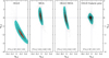 |
Fig. 5 Comparison of the posterior distribution of the microlensing parallax vector, πE, for an inner-large q, u0+ topology fitted to different combinations of datasets (from the left): only OGLE data, only MOA data, combined OGLE and MOA datasets, and OGLE data alone with an incorporated prior on πE based on a Galactic model. The orange region marks the 1σ contour of the two-dimensional distribution, and the turquoise region marks the 2σ contour. |
Settings of the Galactic model (1) used in simulating microlensing events.
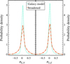 |
Fig. 6 Probability density functions of the two components of the microlensing parallax vector (πE,N in the left panel and πE,E in the right panel), calculated from the Galactic model (Koshimoto et al. 2021a). The dot-dashed turquoise line represents the original function from the simulated events, while the dot-dashed orange function is broadened. The broadened functions are used as priors in the Bayesian inference. |
Lensing parameters, fitted to the OGLE data alone, using a Galactic model prior on πE.
Lensing parameters, fitted to all available datasets.
4 Final multi-instrument data modeling: OGLE, MOA, RoboNet, and MiNDSTEp
4.1 Microlensing parameters
To conclude the analysis of OGLE-2015-BLG-1609 and obtain trustworthy parameters of the system, we fitted 2L1S models with the parallax effect simultaneously to all available data from the four mentioned projects: OGLE, MOA, RoboNet, and MiNDSTEp. In all three topologies (inner-large q, small q, and outer-large q), the models with positive values of u0 had lower values of χ2 statistics. These three models are plotted in Fig. 1, and Fig. 2 shows the same models zoomed in on the planetary anomaly. The corresponding parameters of these models, along with their χ2 statistics, are listed in Table 5. Error bars scaling parameters for corresponding topologies are summarized in Table 6.
4.2 Physical parameters
4.2.1 Source star
Based on the results from the microlensing modeling, the source star is most likely a typical Galactic bulge red giant. In contrast, the blend is a bluer main-sequence star (see Fig. 7). To acquire extinction parameters, we compared the position of the red clump (RC) giants centroid on the CMD to its intrinsic color and brightness. Based on the OGLE-IV photometric maps for the Galactic bulge, calibrated to the standard systems, we selected stars within 2′ of the location of the event and lying on the red giant branch (i.e., with (V − I) > 2.4 mag and 16.1 < I < 16.7 mag; see Fig. 7). This criterion provided a sample of Nstars = 543. Using these stars, we fitted the luminosity function parameterized as in Nataf et al. (2013):
![Mathematical equation: $\[\begin{aligned}N(I) d I= & A ~\exp~ \left[B\left(I-I_{\mathrm{RC}}\right)\right] \\& +\frac{N_{\mathrm{RC}}}{\sqrt{2 \pi} \sigma_{\mathrm{RC}}} \exp \left[-\frac{\left(I-I_{\mathrm{RC}}\right)^2}{2 \sigma_{\mathrm{RC}}^2}\right] \\& +\frac{N_{\mathrm{RGBB}}}{\sqrt{2 \pi} \sigma_{\mathrm{RGBB}}} \exp \left[-\frac{\left(I-I_{\mathrm{RGBB}}\right)^2}{2 \sigma_{\mathrm{RGBB}}^2}\right] \\& +\frac{N_{\mathrm{AGBB}}}{\sqrt{2 \pi} \sigma_{\mathrm{AGBB}}} \exp \left[-\frac{\left(I-I_{\mathrm{AGBB}}\right)^2}{2 \sigma_{\mathrm{AGBB}}^2}\right],\end{aligned}\]$](/articles/aa/full_html/2025/06/aa53454-24/aa53454-24-eq55.png) (7)
(7)
![Mathematical equation: $\[N_{\mathrm{RGBB}}=0.201 \times N_{\mathrm{RC}},\]$](/articles/aa/full_html/2025/06/aa53454-24/aa53454-24-eq89.png) (8)
(8)
![Mathematical equation: $\[N_{\mathrm{AGBB}}=0.028 \times N_{\mathrm{RC}},\]$](/articles/aa/full_html/2025/06/aa53454-24/aa53454-24-eq90.png) (9)
(9)
![Mathematical equation: $\[I_{\mathrm{RGBB}}=I_{\mathrm{RC}}+0.737,\]$](/articles/aa/full_html/2025/06/aa53454-24/aa53454-24-eq91.png) (10)
(10)
![Mathematical equation: $\[I_{\mathrm{AGBB}}=I_{\mathrm{RC}}-1.07,\]$](/articles/aa/full_html/2025/06/aa53454-24/aa53454-24-eq92.png) (11)
(11)
![Mathematical equation: $\[\sigma_{\mathrm{RGBB}}=\sigma_{\mathrm{AGBB}}=\sigma_{\mathrm{RC}},\]$](/articles/aa/full_html/2025/06/aa53454-24/aa53454-24-eq93.png) (12)
where I, σ, and N are the mean magnitude, magnitude dispersion, and number of stars, respectively. The subscripts AGBB denote the asymptotic giant branch bump and RGBB the red giant branch bump. Following Nataf et al. (2013, 2016), we imposed priors summarized in Table 7.
(12)
where I, σ, and N are the mean magnitude, magnitude dispersion, and number of stars, respectively. The subscripts AGBB denote the asymptotic giant branch bump and RGBB the red giant branch bump. Following Nataf et al. (2013, 2016), we imposed priors summarized in Table 7.
To sample the posterior distribution, we used the emcee code. Assuming a Poisson distribution of observed stars, we employed the likelihood function in the form
![Mathematical equation: $\[\ln~ \mathcal{L} \propto-N_{\mathrm{exp}}+\sum_i ~\ln~ N\left(I_i\right) d I.\]$](/articles/aa/full_html/2025/06/aa53454-24/aa53454-24-eq94.png) (13)
(13)
The fitting resulted in IRC = 16.405 ± 0.47 mag and (I − V)RC = 2.93 ± 0.25 mag. As seen in the color-magnitude diagram (Fig. 7), interstellar extinction within the selected 2′ radius is highly differential, which is typical for the Galactic bulge region (Nataf et al. 2013). We estimated the reddening parameters using the values of intrinsic apparent magnitude of the RC calculated by Nataf et al. (2016),
![Mathematical equation: $\[I_{\mathrm{RC}, 0}=14.3955-0.0239 l+0.0122|b|=14.3350 ~\mathrm{mag} \quad \text { and }\]$](/articles/aa/full_html/2025/06/aa53454-24/aa53454-24-eq95.png) (14)
(14)
![Mathematical equation: $\[(V-I)_{\mathrm{RC}, 0}=1.06 ~\mathrm{mag},\]$](/articles/aa/full_html/2025/06/aa53454-24/aa53454-24-eq96.png) (15)
(15)
and found
![Mathematical equation: $\[A_{\mathrm{I}}=2.07 \pm 0.47 ~\mathrm{mag} \quad \text { and } \quad E(V-I)=1.87 \pm 0.25 ~\mathrm{mag}.\]$](/articles/aa/full_html/2025/06/aa53454-24/aa53454-24-eq97.png) (16)
(16)
We combined the reddening with the posterior distribution of the source flux from the microlensing modeling. From this, we obtained the de-reddened color and brightness of the source star. For the inner-large q, u0+ topology we find
![Mathematical equation: $\[I_0=15.211 \pm 0.058 ~\mathrm{mag} \quad \text { and } \quad(V-I)_0=0.96 \pm 0.25 ~\mathrm{mag}.\]$](/articles/aa/full_html/2025/06/aa53454-24/aa53454-24-eq98.png) (17)
(17)
Error bar scaling parameters.
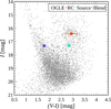 |
Fig. 7 Color–magnitude diagram for stars in the OGLE-IV data within 2′ of the microlensed star in the OGLE-2015-BLG-1609 event. The red circle marks the position of the RC centroid, while the turquoise and purple circles mark the positions of the source and blend, respectively. |
Priors used for the RC centroid fitting.
4.2.2 Source radius
As the color–angular size relations are typically better constrained for the K-band filter, we transformed (V − I)0 of the source to (V − K)0 using color-color relations from Bessell & Brett (1988). To calculate the source angular radius corrected for the limb-darkening, we used relations from Adams et al. (2018):
![Mathematical equation: $\[\log ~\theta_{*, \mathrm{LD}}=0.562 \pm 0.009+0.051 \pm 0.003~(V-K)_0-0.2 ~K_0-~\log~ 2.\]$](/articles/aa/full_html/2025/06/aa53454-24/aa53454-24-eq99.png) (18)
(18)
We assumed that in this relation, as well as in the following ones Eqs. ((20), (21)), the posterior distribution of a given factor is approximated as a normal distribution. Taking the calculated distribution of I0 and (V − I)0 for the inner-large q, u0+ model provided
![Mathematical equation: $\[\theta_{*, \mathrm{LD}}=3.84_{-0.56}^{+0.85} ~\mu \mathrm{as}.\]$](/articles/aa/full_html/2025/06/aa53454-24/aa53454-24-eq100.png) (19)
(19)
4.2.3 Limb-darkening coefficients
To find the effective temperature of the source star, we used the empirical color relations from Houdashelt et al. (2000) for cold giant stars:
![Mathematical equation: $\[\begin{aligned}T_{\text {eff }} & =8556.22 \pm 204.27-5235.57 \pm 352.83~(V-I)_0 \\& +1471.09 \pm 148.20~(V-I)_0^2=4957_{-720}^{+744} \mathrm{~K}.\end{aligned}\]$](/articles/aa/full_html/2025/06/aa53454-24/aa53454-24-eq101.png) (20)
(20)
Estimation of surface gravity was obtained from the Berdyugina & Savanov (1994) relation for G-K giants and subgiants, assuming a solar metallicity for the source:
![Mathematical equation: $\[\begin{aligned}\log ~g= & 8.0 \pm 0.04 ~T_{\text {eff }}+0.31 \pm 0.04 ~M_{0, \mathrm{~V}} \\& +0.27 \pm 0.11~[\mathrm{Fe} / \mathrm{H}]-27.15 \pm 2.1=3.1 \pm 2.2,\end{aligned}\]$](/articles/aa/full_html/2025/06/aa53454-24/aa53454-24-eq102.png) (21)
(21)
where we used M0,V = 1.57 ± 0.27 mag. To derive the limb-darkening coefficients, we used tables from Claret & Bloemen (2011) and assumed solar metallicity and turbulent velocity of 2 km s−1. Those parameters have minor impact on the values of coefficients. For bands in which observational data were collected, we obtained
![Mathematical equation: $\[u_V=0.9198, \quad u_R=0.6535, \quad u_I=0.5597, \quad u_{z^{\prime}}=0.5131.\]$](/articles/aa/full_html/2025/06/aa53454-24/aa53454-24-eq103.png) (22)
(22)
4.2.4 Lens masses and distance
We obtained the angular Einstein radius based on the scaled source radius from finite-source effect modeling and calculated the observed source radius:
![Mathematical equation: $\[\theta_{\mathrm{E}}=\frac{\theta_{*, \mathrm{LD}}}{\rho}=0.46_{-0.24}^{+1.06} ~\mathrm{mas}.\]$](/articles/aa/full_html/2025/06/aa53454-24/aa53454-24-eq104.png) (23)
(23)
Combining this with constraints on the microlensing parallax led to the mass measurement of the host and the companion (Gould 2000):
![Mathematical equation: $\[M_{\mathrm{h}}=\frac{\theta_{\mathrm{E}}}{\kappa \pi_{\mathrm{E}}}=0.17_{-0.12}^{+0.63} ~\mathrm{M}_{\odot} \quad \text { and } \quad M_{\mathrm{c}}=q M_{\mathrm{h}}=0.24_{-0.17}^{+0.90} ~\mathrm{M}_{\mathrm{J}},\]$](/articles/aa/full_html/2025/06/aa53454-24/aa53454-24-eq105.png) (24)
(24)
where κ ≡ 4G/(c2au) ≃ 8.144 mas ![Mathematical equation: $\[\mathrm{M}_{\odot}^{-1}\]$](/articles/aa/full_html/2025/06/aa53454-24/aa53454-24-eq106.png) . Figure 8 presents the full distributions of ρ from the MCMC samples and the corresponding distributions of Mh. Additionally, the source-lens relative parallax is given by
. Figure 8 presents the full distributions of ρ from the MCMC samples and the corresponding distributions of Mh. Additionally, the source-lens relative parallax is given by
![Mathematical equation: $\[\pi_{\mathrm{rel}}=\pi_{\mathrm{E}} \theta_{\mathrm{E}}=0.18_{-0.13}^{+0.51} ~\mathrm{mas},\]$](/articles/aa/full_html/2025/06/aa53454-24/aa53454-24-eq107.png) (25)
(25)
and the relative proper motion by
![Mathematical equation: $\[\mu_{\mathrm{rel}}=\frac{\theta_{\mathrm{E}}}{t_{\mathrm{E}}}=5.7_{-3.0}^{+13.1} ~\mathrm{mas} ~\mathrm{yr}^{-1}.\]$](/articles/aa/full_html/2025/06/aa53454-24/aa53454-24-eq108.png) (26)
(26)
Assuming that the source star is at the typical distance for a Galactic bulge star DS = 8.54 kpc, we estimated the lens distance as
![Mathematical equation: $\[D_{\mathrm{L}}=\frac{\mathrm{au}}{\pi_{\mathrm{rel}}+\pi_{\mathrm{S}}}=3.3_{-2.1}^{+2.6} ~\mathrm{kpc},\]$](/articles/aa/full_html/2025/06/aa53454-24/aa53454-24-eq109.png) (27)
(27)
where πS = 1 / DS. All the values in this section were calculated for the inner-large q, u0+ topology. Results for all the considered models are summarized in Table 8.
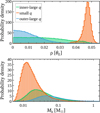 |
Fig. 8 Distributions of the radius of the source (ρ) from MCMC samples and calculated distributions of the mass of the host (Mh) of OGLE-2015-BLG-1609 for different binary lens topologies: inner-large q (blue), small q (orange), and outer-large q (green). |
4.3 Comparison of solutions
Table 5 includes the χ2 values for all three topologies. There is only a minor difference in χ2 between the inner-large q and outer-large q topologies. The small q topology has a slightly lower χ2 (Δχ2 ≈ 10). This difference in χ2 is traced to observations from a single night (HJD = 2457267; Fig. 2). On that night, the rising slope of the planetary anomaly in the small q model fits all the OGLE data points, unlike the other two topologies and unlike other nights, where similar variations occurred between measurements. Specifically, in the case of the small q topology, the four OGLE observations taken that night contribute χ2/d.o.f. = 0.9/4 to the overall χ2/d.o.f. = 3239.4/3405. The OGLE observing logs indicate no anomalous conditions during that night, although such a perfect model fit to the data points seems unlikely and indicates overfitting of the small q topology. Unfortunately, no observations from other projects were collected that night to verify the shape of the light curve seen in the OGLE data.
To quantitatively verify the model topologies, we estimated the Bayesian evidence for each of them. This was done using previously simulated microlensing events from the Galactic model of Koshimoto et al. (2021a) with event input properties given in Table 3. Additionally, from the posterior distribution of θE for each topologies, we derived the corresponding probability density functions. The evidence was then calculated as
![Mathematical equation: $\[\mathcal{Z}=\sum_i p_i w_i \quad \text { with } \quad p_i=f\left(\theta_{\mathrm{E}, i} {\mid} \text {model }\right),\]$](/articles/aa/full_html/2025/06/aa53454-24/aa53454-24-eq110.png) (28)
(28)
where index i denotes i-th simulated event, wi is its weight, and f is derived probability density function for θE for a given model. Evidence values are listed in Table 8. Based on these estimates, only the small q topologies can be considered less probable, while the differences between the outer-large q and inner-large q topologies remains inconclusive.
Considering that 80 MJ is the mass limit for sustaining hydrogen fusion into helium in a stellar core, all topologies suggest that the lens could be a substellar, brown dwarf object. For the two topologies with higher evidence, outer-large q and inner-large q, this probability is estimated to be 49% and 25%, respectively, as shown in Table 8. Using Bayesian evidence values as proportionality indicators, we estimated that the overall probability of the lens being under the 80 MJ mass limit is 34% in the case of the u0+ models. The small q topology provides the best fit to the data and imposes the strongest constraints on ρ, which in turn constrains the host mass (Fig. 8), yielding an extraordinary host mass of Mh = ![Mathematical equation: $\[0.025_{-0.012}^{+0.050}\]$](/articles/aa/full_html/2025/06/aa53454-24/aa53454-24-eq131.png) M⊙.
M⊙.
OGLE-2015-BLG-1609L is the 16th known system found through any of the three major planetary detection methods (transit, radial velocity, and microlensing) whose host is suspected to fall within the brown dwarf mass range (Han et al. 2024). All other systems were also detected through microlensing, which results from the unique capabilities of this method in detecting faint objects. Furthermore, the low mass of the lens suggests that the blended flux cannot be fully explained by the lens’s light contribution.
Physical properties of OGLE-2015-BLG-1609.
4.4 Prospects for follow-up observations
To better characterize the lens system and more accurately constrain the lens mass, additional high-angular-resolution observations will be needed. Out of the three solutions, only the small q solution has well constrained ρ and, consequently, μrel. However, in this solution the μrel is very small and the lens is furthest away and of the lowest mass. The combination of the values of these parameters make the lens undetectable in foreseeable future. On the other hand, both the inner-large q and outer-large q solutions have larger μrel and closer and more massive lenses. We predict that in 2027 the lens-source separation will be ![Mathematical equation: $\[68_{-36}^{+157}\]$](/articles/aa/full_html/2025/06/aa53454-24/aa53454-24-eq132.png) mas for the inner-large q solution. This separation makes the lens potentially detectable with dedicated adaptive optics instruments, which have the angular resolution of of 60 mas (Vandorou et al. 2023)
mas for the inner-large q solution. This separation makes the lens potentially detectable with dedicated adaptive optics instruments, which have the angular resolution of of 60 mas (Vandorou et al. 2023)
Alternatively, use of dual-field interferometer instrument GRAVITY is not possible because of a lack of a bright star (K ≲ 10 mag) for fringe tracking within 30″ of the event’s sky location (Mróz et al. 2025).
5 Summary
We analyzed the microlensing event OGLE-2015-BLG-1609, which shows a planetary anomaly prominent in the surveys data alone. We used a series of modeling approaches, including imposing Galactic model priors, to mitigate challenges such as the unconstrained parallax in the survey data. After incorporating data from the MOA and follow-up projects and refining the OGLE reductions, we identified three possible model topologies for the microlensing system. The two most likely ones have indistinguishable Bayesian evidence. Ultimately, our analysis points to a 34% probability that the lens system is a planet-hosting brown dwarf. We conclude that with a relative proper motion on the order of μrel = 5 mas−1, if the lens’s flux is not resolved in the near future by high-angular-resolution instruments, the probability of the lens being a substellar object will increase.
Acknowledgements
We would like to express our sincere gratitude to the anonymous referee for their careful reading of our manuscript and their insightful comments and suggestions. OGLE Team acknowledges former members of the team, for their contribution to the collection of the OGLE photometric data over the past years. The work by Radosław Poleski was partly supported by the Polish National Agency for Academic Exchange grant “Polish Returns 2019”. The MOA project is supported by JSPS KAKENHI Grant Number JP24253004, JP26247023,JP16H06287 and JP22H00153. YT acknowledges the support of the DFG priority program SPP 1992 “Exploring the Diversity of Extrasolar Planets” (TS 356/3-1). R.F.J. acknowledges support for this project provided by ANID’s Millennium Science Initiative through grant ICN12_009, awarded to the Millennium Institute of Astrophysics (MAS), and by ANID’s Basal project FB210003. L.M. acknowledges financial contribution from PRIN MUR 2022 project 2022J4H55R.
References
- Adams, A. D., Boyajian, T. S., & von Braun, K. 2018, MNRAS, 473, 3608 [NASA ADS] [CrossRef] [Google Scholar]
- Alard, C., & Lupton, R. H. 1998, ApJ, 503, 325 [Google Scholar]
- An, J. H., & Gould, A. 2001, ApJ, 563, L111 [Google Scholar]
- Berdyugina, S. V., & Savanov, I. S. 1994, Astron. Lett., 20, 755 [NASA ADS] [Google Scholar]
- Bessell, M. S., & Brett, J. M. 1988, PASP, 100, 1134 [Google Scholar]
- Bond, I. A., Abe, F., Dodd, R. J., et al. 2001, MNRAS, 327, 868 [Google Scholar]
- Bramich, D. M. 2008, MNRAS, 386, L77 [NASA ADS] [CrossRef] [Google Scholar]
- Claret, A., & Bloemen, S. 2011, A&A, 529, A75 [NASA ADS] [CrossRef] [EDP Sciences] [Google Scholar]
- Crotts, A. P. S., & Tomaney, A. B. 1996, ApJ, 473, L87 [Google Scholar]
- Dominik, M., Jørgensen, U. G., Rattenbury, N. J., et al. 2010, Astron. Nachr., 331, 671 [NASA ADS] [CrossRef] [Google Scholar]
- Foreman-Mackey, D., Hogg, D. W., Lang, D., & Goodman, J. 2013, PASP, 125, 306 [Google Scholar]
- Gaia Collaboration (Vallenari, A., et al.) 2023, A&A, 674, A1 [NASA ADS] [CrossRef] [EDP Sciences] [Google Scholar]
- Gaudi, B. S., & Gould, A. 1997, ApJ, 486, 85 [Google Scholar]
- Goodman, J., & Weare, J. 2010, Commun. Appl. Math. Computat. Sci., 5, 65 [Google Scholar]
- Gould, A. 2000, ApJ, 542, 785 [NASA ADS] [CrossRef] [Google Scholar]
- Gould, A., Dong, S., Gaudi, B. S., et al. 2010, ApJ, 720, 1073 [NASA ADS] [CrossRef] [Google Scholar]
- Gould, A., Han, C., Zang, W., et al. 2022, A&A, 664, A13 [NASA ADS] [CrossRef] [EDP Sciences] [Google Scholar]
- Han, C., Ryu, Y., Lee, C., et al. 2024, A&A, 692, A106 [NASA ADS] [CrossRef] [EDP Sciences] [Google Scholar]
- Houdashelt, M. L., Bell, R. A., & Sweigart, A. V. 2000, AJ, 119, 1448 [Google Scholar]
- Hwang, K.-H., Zang, W., Gould, A., et al. 2022, AJ, 163, 43 [NASA ADS] [CrossRef] [Google Scholar]
- Jung, Y. K., Gould, A., Zang, W., et al. 2019, AJ, 157, 72 [Google Scholar]
- Jung, Y. K., Zang, W., Han, C., et al. 2022, AJ, 164, 262 [NASA ADS] [CrossRef] [Google Scholar]
- Jung, Y. K., Zang, W., Wang, H., et al. 2023, AJ, 165, 226 [NASA ADS] [CrossRef] [Google Scholar]
- Koshimoto, N., & Ranc, C. 2022, https://doi.org/10.5281/zenodo.6869520 [Google Scholar]
- Koshimoto, N., Baba, J., & Bennett, D. P. 2021a, ApJ, 917, 78 [NASA ADS] [CrossRef] [Google Scholar]
- Koshimoto, N., Bennett, D. P., Suzuki, D., & Bond, I. A. 2021b, ApJ, 918, L8 [NASA ADS] [CrossRef] [Google Scholar]
- Lam, C. Y., Lu, J. R., Hosek, Matthew W., J., Dawson, W. A., & Golovich, N. R. 2020, ApJ, 889, 31 [NASA ADS] [CrossRef] [Google Scholar]
- Li, S. S., Zang, W., Udalski, A., et al. 2019, MNRAS, 488, 3308 [NASA ADS] [CrossRef] [Google Scholar]
- Mao, S., & Paczynski, B. 1991, ApJ, 374, L37 [NASA ADS] [CrossRef] [Google Scholar]
- Mróz, P., & Poleski, R. 2024, Exoplanet Occurrence Rates from Microlensing Surveys (Cham: Springer International Publishing), 1 [Google Scholar]
- Mróz, M., Pietrukowicz, P., Poleski, R., et al. 2023, Acta Astron., 73, 127 [Google Scholar]
- Mróz, P., Dong, S., Mérand, A., et al. 2025, ApJ, 980, 47 [Google Scholar]
- Nataf, D. M., Gould, A., Fouqué, P., et al. 2013, ApJ, 769, 88 [Google Scholar]
- Nataf, D. M., Gonzalez, O. A., Casagrande, L., et al. 2016, MNRAS, 456, 2692 [Google Scholar]
- Nunota, K., Koshimoto, N., Suzuki, D., et al. 2024, ApJ, 967, 77 [Google Scholar]
- Paczynski, B. 1986, ApJ, 304, 1 [NASA ADS] [CrossRef] [Google Scholar]
- Penny, M. T., Henderson, C. B., & Clanton, C. 2016, ApJ, 830, 150 [NASA ADS] [CrossRef] [Google Scholar]
- Poleski, R., & Yee, J. C. 2019, Astron. Comput., 26, 35 [NASA ADS] [CrossRef] [Google Scholar]
- Ryu, Y.-H., Udalski, A., Yee, J. C., et al. 2024, AJ, 167, 88 [NASA ADS] [CrossRef] [Google Scholar]
- Schmidt, M. 1968, ApJ, 151, 393 [Google Scholar]
- Shin, I.-G., Yee, J. C., Zang, W., et al. 2023, AJ, 166, 104 [NASA ADS] [CrossRef] [Google Scholar]
- Shin, I.-G., Yee, J. C., Zang, W., et al. 2024, AJ, 167, 269 [NASA ADS] [CrossRef] [Google Scholar]
- Skottfelt, J., Bramich, D. M., Hundertmark, M., et al. 2015, A&A, 574, A54 [NASA ADS] [CrossRef] [EDP Sciences] [Google Scholar]
- Skowron, J., Udalski, A., Kozłowski, S., et al. 2016, Acta Astron., 66, 1 [NASA ADS] [Google Scholar]
- Suzuki, D., Bennett, D. P., Sumi, T., et al. 2016, ApJ, 833, 145 [Google Scholar]
- Terry, S. K., Beaulieu, J.-P., Bennett, D. P., et al. 2024, AJ, 168, 72 [Google Scholar]
- Tsapras, Y. 2018, Geosciences, 8, 365 [NASA ADS] [CrossRef] [Google Scholar]
- Tsapras, Y., Street, R., Horne, K., et al. 2009, Astron. Nachr., 330, 4 [NASA ADS] [CrossRef] [Google Scholar]
- Udalski, A. 2003, Acta Astron., 53, 291 [NASA ADS] [Google Scholar]
- Udalski, A., Szymanski, M. K., Soszynski, I., & Poleski, R. 2008, Acta Astron., 58, 69 [NASA ADS] [Google Scholar]
- Udalski, A., Szymański, M. K., & Szymański, G. 2015, Acta Astron., 65, 1 [NASA ADS] [Google Scholar]
- Udalski, A., Ryu, Y. H., Sajadian, S., et al. 2018, Acta Astron., 68, 1 [NASA ADS] [Google Scholar]
- Vandorou, A., Dang, L., Bennett, D. P., et al. 2023, arXiv e-prints, [arXiv:2302.01168] [Google Scholar]
- Wang, H., Zang, W., Zhu, W., et al. 2022, MNRAS, 510, 1778 [Google Scholar]
- Wozniak, P. R. 2000, Acta Astron., 50, 421 [NASA ADS] [Google Scholar]
- Wyrzykowski, Ł., Kruszyńska, K., Rybicki, K. A., et al. 2023, A&A, 674, A23 [NASA ADS] [CrossRef] [EDP Sciences] [Google Scholar]
- Yang, H., Zhang, X., Hwang, K.-H., et al. 2020, AJ, 159, 98 [Google Scholar]
- Yee, J. C., Shvartzvald, Y., Gal-Yam, A., et al. 2012, ApJ, 755, 102 [Google Scholar]
- Zang, W., Hwang, K.-H., Udalski, A., et al. 2021, AJ, 162, 163 [NASA ADS] [CrossRef] [Google Scholar]
- Zang, W., Yang, H., Han, C., et al. 2022, MNRAS, 515, 928 [NASA ADS] [CrossRef] [Google Scholar]
- Zang, W., Jung, Y. K., Yang, H., et al. 2023, AJ, 165, 103 [CrossRef] [Google Scholar]
All Tables
Lensing parameters, fitted to the OGLE data alone, using a Galactic model prior on πE.
All Figures
|
Fig. 1 Light curves of the microlensing event OGLE-2015-BLG-1609 with three microlensing model topologies for positive values of the impact parameter, u0. The difference between the topologies is visible only during the planetary anomaly (HJD ~ 2457270; see Fig. 2). The photometry comes from the OGLE, MOA, RoboNet, and MiNDSTEp projects. |
| In the text | |
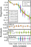 |
Fig. 2 Same as Fig. 1 but for the light curve of the planetary anomaly in OGLE-2015-BLG-1609. |
| In the text | |
|
Fig. 3 Δχ2 map in (log s, log q) parameter space for OGLE-2016-BLG-1609. We named the three visible topologies according to the projected separation: inner-large q (labeled A and delineated by the dashed blue line), small q (B, dot-dashed orange line), and outer-large q (C, dotted green line). Crosses mark the lowest-χ2 models for each topology, and boxes represent the s and q limits used in modeling. |
| In the text | |
|
Fig. 4 Source trajectory and caustics of OGLE-2015-BLG-1609 for different binary lens topologies: inner-large q (blue line), small q (orange line), and outer-large q (green line). The central caustics of the small q and inner-large q models at the point (θx/θE, θy/θE) = (0, 0) are approximately point-like. For clarity, we plot only the small q topology trajectory, as the other trajectories differed only slightly. The orange circle represents the size of the source in the case of the small q topology. |
| In the text | |
|
Fig. 5 Comparison of the posterior distribution of the microlensing parallax vector, πE, for an inner-large q, u0+ topology fitted to different combinations of datasets (from the left): only OGLE data, only MOA data, combined OGLE and MOA datasets, and OGLE data alone with an incorporated prior on πE based on a Galactic model. The orange region marks the 1σ contour of the two-dimensional distribution, and the turquoise region marks the 2σ contour. |
| In the text | |
|
Fig. 6 Probability density functions of the two components of the microlensing parallax vector (πE,N in the left panel and πE,E in the right panel), calculated from the Galactic model (Koshimoto et al. 2021a). The dot-dashed turquoise line represents the original function from the simulated events, while the dot-dashed orange function is broadened. The broadened functions are used as priors in the Bayesian inference. |
| In the text | |
|
Fig. 7 Color–magnitude diagram for stars in the OGLE-IV data within 2′ of the microlensed star in the OGLE-2015-BLG-1609 event. The red circle marks the position of the RC centroid, while the turquoise and purple circles mark the positions of the source and blend, respectively. |
| In the text | |
|
Fig. 8 Distributions of the radius of the source (ρ) from MCMC samples and calculated distributions of the mass of the host (Mh) of OGLE-2015-BLG-1609 for different binary lens topologies: inner-large q (blue), small q (orange), and outer-large q (green). |
| In the text | |
Current usage metrics show cumulative count of Article Views (full-text article views including HTML views, PDF and ePub downloads, according to the available data) and Abstracts Views on Vision4Press platform.
Data correspond to usage on the plateform after 2015. The current usage metrics is available 48-96 hours after online publication and is updated daily on week days.
Initial download of the metrics may take a while.