| Issue |
A&A
Volume 686, June 2024
|
|
|---|---|---|
| Article Number | A234 | |
| Number of page(s) | 11 | |
| Section | Astrophysical processes | |
| DOI | https://doi.org/10.1051/0004-6361/202349063 | |
| Published online | 14 June 2024 | |
OGLE-2018-BLG-0971, MOA-2023-BLG-065, and OGLE-2023-BLG-0136: Microlensing events with prominent orbital effects
1
Department of Physics, Chungbuk National University, Cheongju 28644, Republic of Korea
e-mail: cheongho@astroph.chungbuk.ac.kr
2
Astronomical Observatory, University of Warsaw, Al. Ujazdowskie 4, 00-478 Warszawa, Poland
3
Institute of Natural and Mathematical Science, Massey University, Auckland 0745, New Zealand
4
Korea Astronomy and Space Science Institute, Daejon 34055, Republic of Korea
5
Max Planck Institute for Astronomy, Königstuhl 17, 69117 Heidelberg, Germany
6
Department of Astronomy, The Ohio State University, 140 W. 18th Ave., Columbus, OH 43210, USA
7
University of Canterbury, Department of Physics and Astronomy, Private Bag 4800, Christchurch 8020, New Zealand
8
Department of Particle Physics and Astrophysics, Weizmann Institute of Science, Rehovot 76100, Israel
9
Center for Astrophysics | Harvard & Smithsonian, 60 Garden St., Cambridge, MA 02138, USA
10
Department of Astronomy and Tsinghua Centre for Astrophysics, Tsinghua University, Beijing 100084, PR China
11
School of Space Research, Kyung Hee University, Yongin, Kyeonggi 17104, Republic of Korea
12
Department of Physics, University of Warwick, Gibbet Hill Road, Coventry CV4 7AL, UK
13
Institute for Space-Earth Environmental Research, Nagoya University, Nagoya 464-8601, Japan
14
Code 667, NASA Goddard Space Flight Center, Greenbelt, MD 20771, USA
15
Department of Astronomy, University of Maryland, College Park, MD 20742, USA
16
Department of Earth and Planetary Science, Graduate School of Science, The University of Tokyo, 7-3-1 Hongo, Bunkyo-ku, Tokyo 113-0033, Japan
17
Instituto de Astrofísica de Canarias, Vía Láctea s/n, 38205 La Laguna, Tenerife, Spain
18
Department of Earth and Space Science, Graduate School of Science, Osaka University, Toyonaka, Osaka 560-0043, Japan
19
Department of Physics, The Catholic University of America, Washington, DC 20064, USA
20
Department of Astronomy, Graduate School of Science, The University of Tokyo, 7-3-1 Hongo, Bunkyo-ku, Tokyo 113-0033, Japan
21
Sorbonne Université, CNRS, UMR 7095, Institut d’Astrophysique de Paris, 98 bis bd Arago, 75014 Paris, France
22
Department of Physics, University of Auckland, Private Bag 92019, Auckland, New Zealand
23
University of Canterbury Mt. John Observatory, PO Box 56 Lake Tekapo 8770, New Zealand
Received:
21
December
2023
Accepted:
8
April
2024
Aims. We undertake a project to reexamine microlensing data gathered from high-cadence surveys. The aim of the project is to reinvestigate lensing events whose light curves exhibit intricate anomaly features that are associated with caustics, but lack prior proposed models that would explain these features.
Methods. Through detailed reanalyses considering higher-order effects, we determined that it is vital to account for the orbital motions of lenses to accurately explain the anomaly features observed in the light curves of the lensing events OGLE-2018-BLG-0971, MOA-2023-BLG-065, and OGLE-2023-BLG-0136.
Results. We estimated the masses and distances to the lenses by conducting Bayesian analyses using the lensing parameters of the newly found lensing solutions. These analyses showed that the lenses of the events OGLE-2018-BLG-0971 and MOA-2023-BLG-065 are binaries composed of M dwarfs, while the lens of OGLE-2023-BLG-0136 likely is a binary composed of an early K-dwarf primary and a late M-dwarf companion. For all lensing events, the probability that the lens resides in the bulge is considerably higher than that it is located in the disk.
Key words: gravitational lensing: micro
© The Authors 2024
 Open Access article, published by EDP Sciences, under the terms of the Creative Commons Attribution License (https://creativecommons.org/licenses/by/4.0), which permits unrestricted use, distribution, and reproduction in any medium, provided the original work is properly cited.
This article is published in open access under the Subscribe to Open model. Subscribe to A&A to support open access publication.
1. Introduction
In general, the light curves of microlensing events are modeled by assuming a rectilinear relative motion between the lens and the source. However, deviations from this assumption arise because the accelerations affect the motion of the observer, the lens, or the source. For instance, an observer experiences acceleration due to the Earth’s orbital motion around the Sun, known as microlens-parallax effects (Gould 1992, 2000). Additionally, when a source of a lensing event is part of a binary system in which two stars orbit a common barycenter, the motion of the source is also accelerated (Han & Gould 1997; Rahvar & Dominik 2009). Similarly, the orbital motion of the lens induces acceleration, causing deviations from a rectilinear relative motion between the lens and source. These are known as lens-orbital effects.
In some instances of lensing events, it was crucial to account for the orbital motions of the lens to accurately interpret the observed lensing light curves. MACHO 97-BLG-41 (Alcock et al. 2000) notably marked the first binary-lens single-source (2L1S) system displaying significant deviations from the assumption of a static binary configuration. Initially, these deviations were attributed to the presence of a third body of the lens, specifically, a circumbinary planet (Bennett et al. 1999). However, based on the analysis of an independent data set, Albrow et al. (2000) later proposed a solution involving an orbiting binary lens. The controversy was definitively resolved by Jung et al. (2013), who found through a direct comparison of the two models using a combined data set that the orbiting binary-lens interpretation is preferred over the circumbinary planet model.
OGLE-2006-BLG-109 was the second instance in which orbital effects of the lens played a crucial role in providing accurate explanations for the lensing light curve (Gaudi et al. 2008; Bennett et al. 2010). The light curve of this event exhibited a complex anomaly pattern, comprising multiple distinctive features. A comprehensive understanding of these anomalies was only achieved after combined higher-order effects resulting from the parallactic motion of Earth and the orbital motion of the lens were accounted for. From the analysis considering these higher-order effects, the lens was proven to be the first double-planet system discovered with the gravitational microlensing method.
OGLE-2005-BLG-018 marked the third instance in which the significance of orbital effects of the lens was established. The light curve of the event displayed multiple anomaly features, comprising two neighboring strong anomalies and a comparatively weak anomaly positioned apart from the stronger ones. Although a model based on a static binary lens configuration could approximately explain the two strong anomalies, it was challenging to accurately describe the separate weak anomaly. As a result, this event was not addressed until Shin et al. (2011) revisited it and demonstrated that accounting for the orbital motion of the lens was essential for accurately describing all the anomaly features in the lensing light curve.
Prompted by the work of Shin et al. (2011), Park et al. (2013) revisited microlensing data available until then and conducted thorough analyses of binary-lens events. They focused on cases in which static binary models fell short in accurately describing observed light curves. Through these analyses, they revealed that the substantial residuals of the light curves of the two lensing events OGLE-2006-BLG-277 and OGLE-2012-BLG-0031 from static 2L1S models were predominantly attributed to the influence of an orbital motion of the lens.
OGLE-2009-BLG-020 was identified as a binary-lens event, for which orbital motion was initially predicted through a light-curve analysis (Skowron et al. 2011). The following 3.5 years of radial velocity monitoring confirmed an orbit consistent with the predictions derived from the microlensing light-curve analysis (Yee et al. 2016).
In the case OGLE-2013-BLG-0723, the lensing light curve was initially interpreted by a triple-lens model, in which the lens consisted of a Venus-mass planet and a binary brown dwarf host (Udalski et al. 2015a). Later, Han et al. (2016a) reexamined the event, incorporating orbital effects of the lens, and proposed a revised interpretation involving a two-body lens instead of the previously suggested three-body lens solution. This updated model provided a notably better fit to the observed light curve.
Gaia16aye, detected toward the northern Galactic disk field, was a binary microlensing event and was one of the earliest instances that was detected from the alerts issued by the Gaia space mission. The brightening of the source induced by lensing endured for more than two years, and thus it was crucial to include the orbital motion of the lens for a precise description of the lensing light curve (Wyrzykowski et al. 2020).
The light curve of the lensing event KMT-2021-BLG-0322 exhibited multiple sets of caustic-crossing features. The overall features of the light curve were approximately described by a 2L1S model, but the model left substantial residuals. From the reanalysis, Han et al. (2021) found that the residuals could either be explained by considering a nonrectilinear lens-source motion caused by the combination of microlens-parallax and lens-orbital effects or by adding an additional low-mass companion to the binary lens, and hence three lens components (3L1S system). The degeneracy between the higher-order 2L1S model and the 3L1S model was very severe, making it difficult to determine a correct solution based on the photometric data. This degeneracy was known before for two previous events (MACHO-97-BLG-41 and OGLE-2013-BLG-0723), which led to the false detections of planets in binary systems, and thus, the identification of the degeneracy for the event illustrated that this degeneracy could be common.
In this study, we present comprehensive analyses of three 2L1S lensing events: OGLE-2018-BLG-0971, MOA-2023-BLG-065, and OGLE-2023-BLG-0136. These events are similar. They display anomalies in their light curves with intricate and complex features that prove challenging to interpret using static binary-lens models. We demonstrate that it is important to consider the orbital motions of lenses to precisely describe the observed anomaly features in the lensing light curves.
2. Event selections and data
We undertook a project involving the reexamination of microlensing data obtained from three ongoing high-cadence microlensing surveys: the Korea Microlensing Telescope Network (KMTNet: Kim et al. 2016), the Optical Gravitational Lensing Experiment (OGLE: Udalski et al. 2015a), and the Microlensing Observations in Astrophysics survey (MOA: Bond et al. 2001). In this project, we directed our attention to lensing events that displayed intricate anomaly features related to caustics, but lacked prior proposed models that would explain these features.
We commenced our investigation by analyzing the KMTNet data spanning from the 2016 season to the 2023 season, specifically focusing on identifying anomalous lensing events characterized by conspicuous caustic-crossing features. Subsequently, we examined the lensing models corresponding to these events, filtering out candidate events for which either no models were proposed or for which the presented models failed to accurately delineate the anomalous features. Finally, in the concluding step, we verified the availability of additional data obtained from the OGLE and MOA surveys for the candidate events. Through this process, we identified three lensing events for which the consideration of the orbital motions of the lenses played a crucial role in accurately describing the observed anomaly features in the lensing light curves: OGLE-2018-BLG-0971, MOA-2023-BLG-065, and OGLE-2023-BLG-0136. In Table 1, we present the equatorial and Galactic coordinates of the events. All these events were captured and observed by multiple surveys. We provide the ID references assigned by the respective surveys, using the ID references from the initial discovery surveys in subsequent discussions.
Event coordinates.
Observations of the events by the individual surveys were conducted using the telescopes operated by the respective survey groups. The KMTNet group uses three identical telescopes, each featuring a 1.6-m aperture and equipped with a camera capable of capturing a field spanning 4 square degrees. For a continuous coverage of the lensing events, the KMTNet telescopes are strategically distributed throughout three countries in the Southern Hemisphere: at the Siding Spring Observatory in Australia (KMTA), the Cerro Tololo Interamerican Observatory in Chile (KMTC), and the South African Astronomical Observatory in South Africa (KMTS). The MOA survey employs a telescope with a 1.8-m aperture located at the Mt. John Observatory in New Zealand. The camera mounted on the MOA telescope has the capacity to capture a 2.2 square degree area of the sky in a single shot. The OGLE survey operates the 1.3-m Warsaw telescope situated at the Las Campanas Observatory in Chile. The camera mounted on the OGLE telescope provides a field of view that spans 1.4 square degrees. The primary observations conducted by the KMTNet and OGLE surveys were made in the I band, whereas observations by the MOA survey were conducted in the custom MOA-R band. In all surveys, a portion of the images was acquired in the V band for the color measurements of source stars.
The data of the events were processed using photometry pipelines that are customized to the individual survey groups: KMTNet employed the Albrow et al. (2009) pipeline, OGLE used the Udalski (2003) pipeline, and MOA employed the Bond et al. (2001) pipeline. For the use of the optimal data, the KMTNet data set was refined through a re-reduction process using the code developed by Yang et al. (2024). For each data set, the error bars estimated from the photometry pipelines were recalibrated not only to ensure consistency of the error bars with the scatter of the data, but also to set the χ2 value per degree of freedom (d.o.f.) for each data to unity. This normalization process was made in accordance with the procedure outlined by Yee et al. (2012).
3. Light-curve modeling
The light curves of all the analyzed events show anomalous features that are characteristic of caustics. Caustics arise when a lens system comprises multiple masses, and they represent the source positions at which the magnification of a point source diverges to infinity. Consequently, caustic-related features in the light curves imply that lenses composed of multiple masses produce these events.
Taking the caustic-related features into account, our analysis began by modeling the light curves within a static 2L1S framework. This framework operates under the assumption of rectilinear relative motion between the lens and the source. Within this static binary-lens model, a lensing light curve is defined by seven basic parameters. The first three of these parameters characterizes the approach of the source to the lens, denoted as (t0, u0, tE). These parameters represent the time of the closest lens-source approach, the separation at that instant (impact parameter), and the event timescale, respectively. Here, u0 is scaled to the angular Einstein radius πE, N, and tE is defined as the duration for the source to traverse the Einstein radius. The additional set of three parameters (s, q, α) characterizes the binary lens configuration. These parameters represent the projected separation (scaled to πE, N), the mass ratio of the binary lens components (M1 and M2), and the angle (source trajectory angle) formed between the lens-source proper motion vector μ and the axis defined by M1 and M2. The last parameter ρ, which is defined as the ratio of the angular source radius θ* to the Einstein radius, that is, ρ = θ*/πE, N, quantifies the deformation of lensing light curves during caustic crossings due to finite-source effects. In the 2L1S modeling, we begin by exploring the binary parameters s and q using a grid approach, employing multiple initial values of α. Subsequently, we determine the remaining parameters through a downhill method based on the Markov chain Monte Carlo (MCMC) technique. The lensing solutions are further refined by enabling variation in all parameters.
As shown in the following section, interpreting the light curves of the events examined in this study solely through static 2L1S models poses a significant challenge. In these instances, we undertook additional modeling to account for higher-order effects that might induce deviations in the relative lens-source motion from a rectilinear path. Our modeling approach explored the influences of the orbital motion of the lens and of microlens-parallax effects. To integrate these higher-order effects into the modeling, additional parameters beyond the fundamental set needed to be included. The additional parameters introduced for modeling with microlens-parallax effects encompassed (πE, N, πE, E), representing the north and east components of the microlens-parallax vector, πE, respectively. The microlens-parallax vector is defined as
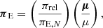
where πrel = au(1/DL − 1/DS) denotes the relative lens-source parallax, and (DL, DS) represent the distances to the lens and source, respectively. Under the first-order approximation of small changes in the positions of the lenses during lensing magnifications, the lens-orbital effects can be characterized by two parameters: (ds/dt, dα/dt). These parameters represent the rates of change in the binary separation and the source trajectory angle, respectively. In the parallax+orbit modeling, we enforced a condition where the projected kinetic-to-potential energy ratio was required to remain below unity. This condition ensured that the planet remained gravitationally bound to its host. The energy ratio was computed from the higher-order lensing parameters by
![$$ \begin{aligned} \left( {\mathrm{KE}\over \mathrm{PE}}\right)_\perp = {(a_\perp /\mathrm{au})^3 \over 8\pi ^2(M/M_\odot )} \left[ \left( {1\over s} {\mathrm{d}s/\mathrm{d}t\over \mathrm{yr}^{-1}}\right)^2+ \left( {\mathrm{d}\alpha /\mathrm{d}t \over \mathrm{yr}^{-1}}\right)^2 \right]. \end{aligned} $$](/articles/aa/full_html/2024/06/aa49063-23/aa49063-23-eq2.gif)
Here, a⊥ denotes the physical separation between the binary lens components. The Keplerian orbital motion can only be fully described when additional parameters are included1. However, determining these additional parameters poses a challenge because gravitational lensing is limited and is therefore insensitive to the motion of the lens along the line of sight, and the partial light-curve coverage spans only a minor fraction of the rotation period (Albrow et al. 2000).
Another higher-order effect that accelerates the relative lens-source motion is the orbital motion of the source, known as the “xallarap effect” (Griest & Hu 1992; Han & Gould 1997; Poindexter et al. 2005; Zhu et al. 2017; Satoh et al. 2023). While the lens is confirmed to be binary, there is no prior justification to assume a binary source, although this possibility cannot be entirely dismissed. Therefore, we refrained from testing the xallarap effect as long as the observed anomalies can be explained by lens-orbital effects.
On occasion, the light curves of 2L1S events affected by higher-order effects can imitate the patterns seen in 3L1S event light curves. This confusion typically arises when a distinct anomaly feature in a lensing light curve is isolated from the primary ones, as seen in previous events such as MACHO-97-BLG-41, OGLE-2013-BLG-0723, and KMT-2021-BLG-0322. For the events we analyzed here, we find no such degeneracies. In the following subsections, we offer detailed analyses of each individual event.
3.1. OGLE-2018-BLG-0971
The OGLE group first identified the lensing event OGLE-2018-BLG-0971 on 4 June 2018. Four days later, the MOA group verified the event, and the KMTNet group later retrieved it from a post-season data examination. The MOA and KMTNet groups designated the event MOA-2018-BLG-173 and KMT-2018-BLG-2336, respectively. Figure 1 shows the light curve of the event. The source of the event was situated within the overlapping region of the three KMTNet fields BLG02, BLG03, and BLG43. To differentiate between the individual data sets, we designated labels corresponding to the respective fields. The light curve shows multiple anomaly features centered at HJD ≡ HJD − 2400000 ∼ 58 277 (t1), ∼58 280 (t2), and ∼58 283 (t3). The symmetric pattern with respect to t1 suggests that the anomaly around this epoch likely stems from the approach of the source to a caustic cusp, while the U-shaped pattern spanning t2 to t3 indicates that these epochs correspond to the times of the caustic entrance and exit. In addition to these anomaly features, a subtle anomaly feature appears just after the caustic exit. Figure 2 offers a detailed view of this specific region.
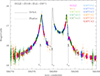 |
Fig. 1. Light curve of the lensing event OGLE-2018-BLG-0971. The solid and dotted curves drawn over the data points represent the model curves obtained from the 2L1S analyses with and without the orbital motion of the lens, respectively. The arrows labeled t1, t2, and t3 denote the times of the major anomaly features. |
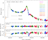 |
Fig. 2. Enlarged view of the OGLE-2018-BLG-0971 light curve in the region around t2 and t3 marked in Fig. 2. |
After modeling the light curve using a static 2L1S framework, we identified a solution that broadly captures the features of the anomaly. In Table 2, we list the lensing parameters of the static solution. However, the static model exhibits subtle residuals, particularly in the vicinity of t3, as illustrated in the magnified view presented in Fig. 2.
Lensing parameters of OGLE-2018-BLG-0971.
In light of the deviations from the static model, we checked the feasibility of explaining the deviation with higher-order effects. The event duration, estimated as tE ∼ 7.1 days from the static model, is short. Consequently, we initially considered the lens-orbital effect in the modeling. Through this approach, we derived a solution that accounts for all anomaly features. The model curve of this solution is shown as a solid line in Fig. 1, offering a comprehensive view, and in Fig. 2, providing an enlarged view around t3. The fit significantly improved with the inclusion of lens orbital motion, by Δχ2 = 3949.4 compared to the static model. Subsequent examination of microlens-parallax effects through additional modeling revealed a very slight improvement in the fit of Δχ2 = 0.9, indicating the predominant influence of lens-orbital effects. In Fig. 3, we plot the scatter plot of points in the MCMC chain on the πE, E–πE, N plane. In Table 2, we provide the lensing parameters for the orbit-only and for the orbit+parallax solutions. The parameters defining the binary lens are (s, q)∼(1.01, 0.87), indicating that the event was generated a binary system composed of roughly equal masses with a separation close to the Einstein radius of the lens system. Although the timescale of the event, tE ∼ 7.1 days, represents only a small fraction of the Earth’s orbital period, we conducted separate modeling specifically to account for the microlens-parallax effect. From this analysis, it was observed that not only did the fit perform worse compared to the orbit-only model by Δχ2 = 42.6, but that the derived parallax parameters (πE, E, πE, N)∼(35.80, 32.50) also appeared to be absurdly large for a typical Galactic lensing event.
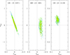 |
Fig. 3. Scatter plots of points in the MCMC chain on the πE, E–πE, N planes for the four events analyzed in this paper. The points are color-coded to represent those with < 1σ (red), < 2σ (yellow), < 3σ (green), and < 4σ (cyan). |
The configuration of the lens system for the lensing event OGLE-2018-BLG-0971 is shown in Fig. 4. This configuration reveals that the lens system forms a single set of resonant caustics featuring six cusps: two along the binary axis, and four positioned away from the axis. The source initially approached the left on-axis cusp around t1, entered the caustic near t2, and exited the caustic at around t3. These caustic approaches and crossings gave rise to anomalies at the corresponding epochs. The primary deviation of the static 2L1S model, particularly around t3, stems from its inability to account for the variation in the caustic caused by the orbital motion of the binary lens.
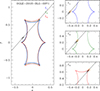 |
Fig. 4. Lens system configuration for OGLE-2018-BLG-0971. The diagonal line with the arrow represents the source trajectory, and the closed figures composed of concave curves represent caustics. The caustic shape and location evolve over time due to the orbital motion of the lens. The sets of caustics drawn in black, green, and red correspond to the three anomaly epochs t1, t2, and t3 marked in Fig. 1. The right panels display still frames capturing the approach of the source to the caustic at these three epochs. The size of the orange circle on the source trajectory that appears in each right panel indicates the angular dimension of the source relative to the size of the caustic. |
3.2. MOA-2023-BLG-065
Figure 5 shows the lensing light curve of the MOA-2023-BLG-065 event. The source flux magnification induced by lensing was initially identified on 17 March 2023 (HJD′ = 60 021), through the survey conducted by the MOA group. It was subsequently confirmed by the KMTNet group. The ID reference designated by the KMTNet survey is KMT-2023-BLG-2430. The light curve displays a complex pattern comprising multiple anomaly features. Notably, two spike features at t1 ∼ 60 020 and t3 ∼ 60 035 appear to be a pair of caustic-crossing spikes. Furthermore, the symmetry observed between the ascending and descending segments of the anomaly feature centered at t4 ∼ 60 043 implies that it originated from the approach of the source to a cusp of the caustic. While the magnification between caustic spikes typically follows a U-shaped pattern, the region between the caustic spikes at t1 and t3 deviates significantly from a U-shape, displaying a distinctive rise and fall in the region centered at t2 ∼ 60 023. This deviation is indicative of a source that asymptotically approaches a fold of the caustic.
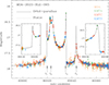 |
Fig. 5. Lensing light curve of MOA-2023-BLG-065. The left and right insets show the zoom-in views of the regions around the caustic spikes at t1 and t3. |
From the 2L1S analysis of the lensing light curve under a static binary frame, we found that the model falls short of precisely describing the data, even though it outlines the anomaly features approximately. In Fig. 5, the static 2L1S model is represented by the dotted curve. This static model exhibits a notably inadequate fit especially in the region of the anomaly centered at t4, as highlighted in the enlarged view presented in Fig. 6. The complete lensing parameters for the static 2L1S solution are detailed in Table 3.
Lensing parameters of MOA-2023-BLG-065.
Although the static solution cannot describe the anomaly feature at around t4 adequately, it exhibits an anomaly around the time of that anomaly. This suggests the possibility that it can be described with a slight deformation of the source trajectory caused by higher-order effects. In light of this possibility, we conducted three additional sets of modeling: The first two models separately incorporated microlens-parallax and lens-orbital effects, and the third model encompassed both effects simultaneously. In Table 3, we present the lensing parameters for the three models. Comparison of the static and higher-order solution demonstrates a notable enhancement in the fit, with a Δχ2 = 526.4 compared to the static solution. In Fig. 3, we present the scatter plot of points in the MCMC chain on the πE, E–πE, N plane. It shows that the east component of the microlens-parallax vector, πE, E, is constrained, although the uncertainty of the north component, πE, N, is large. Additionally, the normalized source radius ρ = (1.739 ± 0.037)×10−3 was measured from the deformation of the light curve by finite source effects during the epochs around t2 and t3. The magnified views of these specific regions are shown in the two insets of Fig. 5.
Figure 7 illustrates the lens-system configuration of MOA-2023-BLG-065. It shows that the binary lens, characterized by parameters (s, q)∼(1.5, 0.9), creates a resonant caustic, and the source traversed the left side of this caustic. Initially, the source passed the upper fold, creating the first caustic spike at t1. Subsequently, it approached the upper left fold asymptotically, resulting in rising and falling features around t2. The source then exited the caustic, generating the second caustic spike at t3, and proceeded to pass the tip of the lower left cusp, causing the final anomaly feature at around t4. The distortion of the caustic due to the orbital motion of the lens led the light curve to deviate from the anticipated behavior according to the static model. This discrepancy was particularly noticeable in the part of the light curve during the final approach of the cusp, enabling the detection of the orbital effect of the lens.
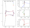 |
Fig. 7. Lens system configuration for MOA-2023-BLG-065. |
3.3. OGLE-2023-BLG-0136
The lensing event OGLE-2023-BLG-0136 was first found during its early phase by the OGLE group on 1 April 2023 (HJD′ = 60 036). Subsequently, the KMTNet survey validated the event, designating it KMT-2023-BLG-2849. Figure 8 illustrates the lensing light curve of the event. The curve exhibits a complex pattern of anomalies, comprised of multiple distinct features: a caustic-crossing feature around t1 = 59 997, and two additional features centered at around t2 = 60 089 and t3 = 60 103. The coverage of the first feature was limited because it was only observed by the KMTC telescope, while the other KMTNet telescopes and the OGLE telescope had not started their observations of the 2023 season at the time of the anomaly. However, the subsequent two anomaly features were extensively observed by the combined data from both the OGLE and KMTNet surveys.
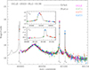 |
Fig. 8. Lensing light curve of OGLE-2023-BLG-0136. The insets provides closer look at the regions surrounding t2 and t3. |
We initially modeled the lensing light curve under a static 2L1S framework. The model curve of the static solution is depicted as the dotted curve in Fig. 8, and the lensing parameters of the solution are listed in Table 4. Upon examination of the fit, it is observed that this model roughly captures the anomaly features around t2 and t3, but it explains the feature at t1 inaccurately. Figure 9 offers a closer look at the model fit around t1. While the static model does not capture the first caustic-crossing anomaly precisely, it displays a weak bump feature that seems to result from a caustic approach. This suggests that the source might pass over the caustic, potentially influenced by a slight shift in the caustic position due to the orbital motion of the binary lens. Considering this, we continued with additional modeling that incorporated the effects of the orbital motion of the lens.
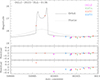 |
Fig. 9. Enlarged view of the OGLE-2023-BLG-0136 light curve in the region around t1 marked in Fig. 8. |
Lensing parameters of OGLE-2023-BLG-0136.
The solid curves in Figs. 8 and 9 represent the model derived from the orbital solution. The lensing parameters of the solution are listed in Table 4. From the inspection of the fit, it is found that the orbital solution accurately accounts for the anomaly around t1, improving the fit by Δχ2 = 2367.4 compared to the static solution. The estimated event timescale, tE ∼ 60 days, is moderately long, and thus we further examined whether incorporating the microlens-parallax effect could enhance the fit. From the model derived with the two higher-order effects, we found a marginal enhancement in the fit, Δχ2 = 4.5, compared to the orbital solution. This suggests that the dominant higher-order effect is attributed to the orbital motion of the lens. The details of the lensing parameters for the parallax and orbit+parallax solutions are outlined in Table 4 and the scatter plot on the πE, E–πE, N plane is shown in Fig. 3. The estimated binary lens parameters are (s, q)∼(0.71, 0.30). The normalized source radius, ρ = (2.005 ± 0.029)×10−3, was measured precisely from the deformed light curve during the anomaly at around t2. The enlarged view of this region is shown in the inset of Fig. 8.
In Fig. 10, we illustrate the lens system configuration for OGLE-2023-BLG-0136. At the time of the first anomaly, the caustic exhibited a resonant form in which the central caustic and peripheral caustics were interconnected by narrow bridges. The first anomaly feature at around t1 was generated when the source traversed the lower bridge of this resonant caustic. As the source proceeded, the binary separation decreased, leading to the detachment of the peripheral caustics from the central caustic. The second and third anomaly features arose from the successive passages of the source over the lower and right cusps of the upper peripheral caustic. The static model effectively captured the second and third anomaly features due to their close temporal proximity, which minimized the deformation of the caustic caused by the lens orbital motion. However, the time gap between these features and the first anomaly feature exceeded 100 days, resulting in substantial alterations to the caustic shape and position. As a result, the static model fell short in accurately representing the observed light curve.
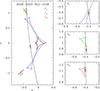 |
Fig. 10. Configuration of the lens system for OGLE-2023-BLG-0136. |
It is important to note that event timescales can vary significantly between static and nonstatic models. For instance, in the case of MOA-2023-BLG-065, the timescale shifts from ∼30.7 days for the static solution to ∼37.8 days for the higher-order solution. Similarly, for OGLE-2023-BLG-0136, the timescale changes from ∼66.7 days for the static solution to ∼59.4 days for the higher-order solution. The timescale serves as a fundamental observable for constraining the physical parameters of the lens. Therefore, accounting for higher-order effects in modeling is essential to determine these parameters accurately.
4. Source stars and Einstein radii
In this section, we specify the source stars and determine the angular Einstein radii of the events. The source stars were specified based on their colors and magnitudes, and we accounted for corrections due to reddening and extinction. In this process, we first conducted photometry of the I and V band data using the pyDIA code (Albrow 2017), and we then estimated the instrumental source color and magnitude, (V − I, I)S, by regressing the data of the individual passbands with respect to the model. The calibration of the source color and magnitude followed the method outlined by Yoo et al. (2004), leveraging the centroid of the red giant clump (RGC) in the color-magnitude diagram (CMD) for this purpose. The RGC centroid can be used for reference because its de-reddened color and magnitude, represented as (V − I, I)RGC, 0, were established by Bensby et al. (2013) and Nataf et al. (2013). In the calibration process, we first positioned the source in the CMD constructed using the pyDIA code, measured the offsets of the source in color and magnitude, Δ(V − I, I), from the RGC centroid, and then estimated the dereddened source color and magnitude as

In Fig. 11, we indicate the locations of source stars for the individual events relative to the RGC centroids on the instrumental CMDs constructed using the KMTC data sets. The values estimated for (V − I, I)S, (V − I, I)RGC, (V − I, I)RGC, 0, and (V − I, I)S, 0 through the described procedure are compiled in Table 5. Based on the derived colors and magnitudes, we determine that the source star of OGLE-2018-BLG-0971 is a K-type subgiant. Additionally, the sources of MOA-2023-BLG-065 and OGLE-2023-BLG-0136 are G-type main-sequence stars.
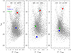 |
Fig. 11. Positions of source stars with respect to the centroids of the RGC in the instrumental CMDs. For MOA-2023-BLG-065 and OGLE-2023-BLG-0136, the positions of the blends are also marked. |
Source parameters, Einstein radii, and relative proper motions.
The angular Einstein radius of each event was estimated from the relation

where the angular source radius θ* was deduced from the color and magnitude, and the normalized source radius ρ was measured from the light-curve analysis. To derive the source radius, we initially transformed the measured V − I color into V − K color using the Bessell & Brett (1988) relation. Subsequently, we determined θ* using the relation provided by Kervella et al. (2004) between (V − K, V) and θ*. The estimated angular radii of source stars for the individual lensing events are listed in Table 5, along with the corresponding angular Einstein radii calculated using the relation described in Eq. (4). The relative lens-source proper motions estimated by the relation

are also listed in the table.
For MOA-2023-BLG-065 and OGLE-2023-BLG-0136, we were able to constrain the blended light. In Fig. 11, we mark the positions of blend in the CMDs. To assess the likelihood of the lens being the primary source of the blended flux, we measured the centroids of the source image during lensing magnification and at the baseline. In the case of MOA-2023-BLG-065, the measured astrometric offset between the source positions is δθ = 0.46 ± 0.08 arcsec. This excludes the possibility that the blended light comes mainly from the lens. For OGLE-2023-BLG-0136, the significant astrometric uncertainty prevents us from drawing a meaningful conclusion regarding the origin of the blended light.
5. Physical lens parameters
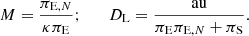
The physical parameters of a lens are constrained by the lensing observables tE, πE, N, and πE. When all these parameters are measured simultaneously, the mass and distance to the lens are uniquely determined by
Here, κ = 4G/(c2au) and πS = au/DS represent the parallax of the source lying at a distance DS (Gould 2000). For all analyzed events, the observables of tE and πE, N were measured precisely, but the constraint on the microlens parallax was relatively weak because of its subtle effects. Due to these incomplete measurements of the lensing observables, we determined the physical lens parameters through Bayesian analyses of the individual events. This approach integrates constraints from measured lensing observables with priors derived from the physical and dynamic distributions, as well as the mass function of lens objects within the Galaxy.
The Bayesian analysis began by generating a large number of synthetic events via a Monte Carlo simulation. Within this simulation, the physical parameters of the lens mass were deduced from a model mass function, while the distances to the lens and source, along with their relative proper motion, were derived from a Galaxy model. Our approach incorporated the mass function model suggested by Jung et al. (2018) and used the Galaxy model introduced by Jung et al. (2021). For each synthetic event defined by physical parameters (Mi, DL, i, DS, i, μi), we calculated the values of the corresponding lensing observables using the relations
for the event timescale and Einstein radius, respectively, and using the relation in Eq. (1) for the microlens parallax. Then, the posteriors of M and DL were obtained by assigning a weight to each event of  , where the
  value was computed by
Here, ΔtE, i = tE, i − tE, ΔθE, i = θE, i − πE, N, (tE, πE, N) stand for the measured values of the observables, [σ(tE),σ(πE, N)] indicate their corresponding uncertainties, and bj, k represents the inverse covariance matrix of the microlens-parallax vector πE, (πE, 1, πE, 2)i = (πE, N, πE, E)i are the parallax parameters of each simulated event, and (πE, N, πE, E) represents the parallax parameters measured from the modeling. Han et al. (2016b) showed that parallax measurements can be important even when there is little improvement in the χ2 because they can constrain πE to be small. We therefore considered the constraints given by the measured parallax parameters in the Bayesian analyses.
In Figs. 12 and 13, we present the Bayesian posteriors of the primary lens masses and distances to the lens systems. In Table 6, we summarize the estimated physical parameters for the individual lensing events. Among the parameters, M1 and M2 denote the masses of the primary and companion of the lens, and a⊥ denotes the projected physical separation between M1 and M2. We present the median value derived from the Bayesian posterior distribution as a representative value for each physical parameter, with uncertainties estimated within the 16%–84% range of the distribution. The table also lists the relative probabilities for the lens being in the Galactic disk, pdisk, and in the bulge, pbulge. According to the estimated masses, the lenses of the events OGLE-2018-BLG-0971 and MOA-2023-BLG-065 are binaries composed of M dwarfs. On the other hand, the lens of OGLE-2023-BLG-0136 is likely to be a binary composed of an early K-dwarf primary and a late M-dwarf companion. Across all the analyzed events, pbulge is substantially higher than pdisk, suggesting a higher likelihood of the all lenses being located in the bulge rather than the disk. The probabilities pdisk and pbulge were found by analyzing the proportion of artificial lensing events where the lenses came from either the disk or bulge distributions within the Galaxy model used in the Monte Carlo simulation process.
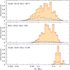 |
Fig. 12. Bayesian posterior distributions of the primary lens mass (M1) for the lensing events. In each panel, the event rate contributions from the disk and bulge lens populations are depicted by the blue and red curves, respectively, and the black curve represents the sum of the contributions from two lens populations. |
 |
Fig. 13. Bayesian posterior distributions of the distances to the lens (DL). The notations correspond to those used in Fig. 12. |
Physical lens parameters.
6. Summary
We have analyzed microlensing data collected from high-cadence surveys to reevaluate lensing events that lacked proposed interpretations for their intricate anomaly features. Through detailed reanalyses considering higher-order effects, we identified that it is vital to account for the orbital motions of lenses to accurately explain the anomaly features observed in the lensing light curves of OGLE-2018-BLG-0971, MOA-2023-BLG-065, and OGLE-2023-BLG-0136.
By conducting Bayesian analyses based on the lensing parameters from the newly found solutions and together with the constraints derived from lensing observables, we estimated the masses and distances to the lenses. These analyses revealed that the lenses for events OGLE-2018-BLG-0971 and MOA-2023-BLG-065 are binary systems consisting of M dwarfs. Additionally, for OGLE-2023-BLG-0136, the lens is likely to be a binary system comprising an early K-dwarf primary and a late M-dwarf companion. Notably, across all observed lensing events, the likelihood of the lens being in the bulge significantly outweighs its likelihood of being in the disk.
To access a comprehensive description of the orbital lensing parameters, we refer to the summary provided in the appendix of Skowron et al. (2011).
Acknowledgments
Work by C.H. was supported by the grants of National Research Foundation of Korea (2019R1A2C2085965). J.C.Y. and I.-G.S. acknowledge support from U.S. NSF Grant No. AST-2108414. Y.S. acknowledges support from BSF Grant No. 2020740. This research has made use of the KMTNet system operated by the Korea Astronomy and Space Science Institute (KASI) at three host sites of CTIO in Chile, SAAO in South Africa, and SSO in Australia. Data transfer from the host site to KASI was supported by the Korea Research Environment Open NETwork (KREONET). This research was supported by KASI under the R&D program (project No. 2023-1-832-03) supervised by the Ministry of Science and ICT. W.Z. and H.Y. acknowledge support by the National Natural Science Foundation of China (Grant No. 12133005). W. Zang acknowledges the support from the Harvard-Smithsonian Center for Astrophysics through the CfA Fellowship. The MOA project is supported by JSPS KAKENHI Grant Number JP24253004, JP26247023, JP16H06287 and JP22H00153.
References
- Albrow, M. 2017, https://doi.org/10.5281/zenodo.268049 [Google Scholar]
- Albrow, M. D., Beaulieu, J.-P., Caldwell, J. A. R., et al. 2000, ApJ, 534, 894 [NASA ADS] [CrossRef] [Google Scholar]
- Albrow, M., Horne, K., Bramich, D. M., et al. 2009, MNRAS, 397, 2099 [Google Scholar]
- Alcock, C., Allsman, R. A., Alves, D., et al. 2000, ApJ, 541, 270 [NASA ADS] [CrossRef] [Google Scholar]
- Bennett, D. P., Rhie, S. H., Becker, A. C., et al. 1999, Nature, 402, 57 [NASA ADS] [CrossRef] [Google Scholar]
- Bennett, D. P., Rhie, S. H., Nikolaev, S., et al. 2010, ApJ, 713, 837 [Google Scholar]
- Bensby, T., Yee, J. C., Feltzing, S., et al. 2013, A&A, 549, A147 [NASA ADS] [CrossRef] [EDP Sciences] [Google Scholar]
- Bessell, M. S., & Brett, J. M. 1988, PASP, 100, 1134 [Google Scholar]
- Bond, I. A., Abe, F., Dodd, R. J., et al. 2001, MNRAS, 327, 868 [Google Scholar]
- Gaudi, B. S., Bennett, D. P., Udalski, A., et al. 2008, Science, 319, 927 [Google Scholar]
- Gould, A. 1992, ApJ, 392, 442 [Google Scholar]
- Gould, A. 2000, ApJ, 542, 785 [NASA ADS] [CrossRef] [Google Scholar]
- Griest, K., & Hu, W. 1992, ApJ, 397, 362 [Google Scholar]
- Han, C., & Gould, A. 1997, ApJ, 480, 196 [NASA ADS] [CrossRef] [Google Scholar]
- Han, C., Bennett, D. P., Udalski, A., et al. 2016a, ApJ, 825, 8 [NASA ADS] [CrossRef] [Google Scholar]
- Han, C., Udalski, A., Gould, A., et al. 2016b, ApJ, 828, 53 [NASA ADS] [CrossRef] [Google Scholar]
- Han, C., Gould, A., Hirao, Y., et al. 2021, A&A, 655, A24 [NASA ADS] [CrossRef] [EDP Sciences] [Google Scholar]
- Jung, Y. K., Han, C., Gould, A., et al. 2013, ApJ, 768, L7 [NASA ADS] [CrossRef] [Google Scholar]
- Jung, Y. K., Udalski, A., Gould, A., et al. 2018, AJ, 155, 219 [Google Scholar]
- Jung, Y. K., Han, C., Udalski, A., et al. 2021, AJ, 161, 293 [NASA ADS] [CrossRef] [Google Scholar]
- Kervella, P., Thévenin, F., Di Folco, E., & Ségransan, D. 2004, A&A, 426, 29 [Google Scholar]
- Kim, S.-L., Lee, C.-U., Park, B.-G., et al. 2016, JKAS, 49, 37 [Google Scholar]
- Nataf, D. M., Gould, A., Fouqué, P., et al. 2013, ApJ, 769, 88 [Google Scholar]
- Park, H., Udalski, A., Han, C., et al. 2013, ApJ, 778, 134 [NASA ADS] [CrossRef] [Google Scholar]
- Poindexter, S., Afonso, C., Bennett, D. P., et al. 2005, ApJ, 633, 914 [NASA ADS] [CrossRef] [Google Scholar]
- Rahvar, S., & Dominik, M. 2009, MNRAS, 392, 1193 [CrossRef] [Google Scholar]
- Satoh, Y. K., Koshimoto, N., Bennett, D. P., et al. 2023, AJ, 166, 116 [CrossRef] [Google Scholar]
- Shin, I.-G., Udalski, A., Han, C., et al. 2011, ApJ, 735, 85 [NASA ADS] [CrossRef] [Google Scholar]
- Skowron, J., Udalski, A., Gould, A., et al. 2011, ApJ, 738, 87 [Google Scholar]
- Smith, M. C., Mao, S., & Paczyński, B. 2003, MNRAS, 339, 925 [NASA ADS] [CrossRef] [Google Scholar]
- Udalski, A. 2003, Acta Astron., 53, 291 [NASA ADS] [Google Scholar]
- Udalski, A., Jung, Y. K., Han, C., et al. 2015a, ApJ, 812, 47 [NASA ADS] [CrossRef] [Google Scholar]
- Udalski, A., Szymański, M. K., Szymański, G., et al. 2015b, Acta Astron., 65, 1 [NASA ADS] [Google Scholar]
- Wyrzykowski, Ł., Mróz, P., Rybicki, K. A., et al. 2020, A&A, 633, A98 [NASA ADS] [CrossRef] [EDP Sciences] [Google Scholar]
- Yang, H., Yee, J. C., Hwang, K. H., et al. 2024, MNRAS, 528, 11 [NASA ADS] [CrossRef] [Google Scholar]
- Yee, J. C., Shvartzvald, Y., Gal-Yam, A., et al. 2012, ApJ, 755, 102 [Google Scholar]
- Yee, J. C., Johnson, J. A., Skowron, J., et al. 2016, ApJ, 821, 121 [NASA ADS] [CrossRef] [Google Scholar]
- Yoo, J., DePoy, D. L., Gal-Yam, A., et al. 2004, ApJ, 603, 139 [Google Scholar]
- Zhu, W., Udalski, A., Novati, S. C., et al. 2017, AJ, 154, 210 [NASA ADS] [CrossRef] [Google Scholar]
All Tables
All Figures
|
Fig. 1. Light curve of the lensing event OGLE-2018-BLG-0971. The solid and dotted curves drawn over the data points represent the model curves obtained from the 2L1S analyses with and without the orbital motion of the lens, respectively. The arrows labeled t1, t2, and t3 denote the times of the major anomaly features. |
| In the text | |
|
Fig. 2. Enlarged view of the OGLE-2018-BLG-0971 light curve in the region around t2 and t3 marked in Fig. 2. |
| In the text | |
|
Fig. 3. Scatter plots of points in the MCMC chain on the πE, E–πE, N planes for the four events analyzed in this paper. The points are color-coded to represent those with < 1σ (red), < 2σ (yellow), < 3σ (green), and < 4σ (cyan). |
| In the text | |
|
Fig. 4. Lens system configuration for OGLE-2018-BLG-0971. The diagonal line with the arrow represents the source trajectory, and the closed figures composed of concave curves represent caustics. The caustic shape and location evolve over time due to the orbital motion of the lens. The sets of caustics drawn in black, green, and red correspond to the three anomaly epochs t1, t2, and t3 marked in Fig. 1. The right panels display still frames capturing the approach of the source to the caustic at these three epochs. The size of the orange circle on the source trajectory that appears in each right panel indicates the angular dimension of the source relative to the size of the caustic. |
| In the text | |
|
Fig. 5. Lensing light curve of MOA-2023-BLG-065. The left and right insets show the zoom-in views of the regions around the caustic spikes at t1 and t3. |
| In the text | |
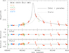 |
Fig. 6. Enlarged view of the MOA-2023-BLG-065 light curve in the region around t4 marked in Fig. 5. |
| In the text | |
|
Fig. 7. Lens system configuration for MOA-2023-BLG-065. |
| In the text | |
|
Fig. 8. Lensing light curve of OGLE-2023-BLG-0136. The insets provides closer look at the regions surrounding t2 and t3. |
| In the text | |
|
Fig. 9. Enlarged view of the OGLE-2023-BLG-0136 light curve in the region around t1 marked in Fig. 8. |
| In the text | |
|
Fig. 10. Configuration of the lens system for OGLE-2023-BLG-0136. |
| In the text | |
|
Fig. 11. Positions of source stars with respect to the centroids of the RGC in the instrumental CMDs. For MOA-2023-BLG-065 and OGLE-2023-BLG-0136, the positions of the blends are also marked. |
| In the text | |
|
Fig. 12. Bayesian posterior distributions of the primary lens mass (M1) for the lensing events. In each panel, the event rate contributions from the disk and bulge lens populations are depicted by the blue and red curves, respectively, and the black curve represents the sum of the contributions from two lens populations. |
| In the text | |
|
Fig. 13. Bayesian posterior distributions of the distances to the lens (DL). The notations correspond to those used in Fig. 12. |
| In the text | |
Current usage metrics show cumulative count of Article Views (full-text article views including HTML views, PDF and ePub downloads, according to the available data) and Abstracts Views on Vision4Press platform.
Data correspond to usage on the plateform after 2015. The current usage metrics is available 48-96 hours after online publication and is updated daily on week days.
Initial download of the metrics may take a while.