| Issue |
A&A
Volume 674, June 2023
|
|
|---|---|---|
| Article Number | A89 | |
| Number of page(s) | 10 | |
| Section | Planets and planetary systems | |
| DOI | https://doi.org/10.1051/0004-6361/202346166 | |
| Published online | 07 June 2023 | |
MOA-2022-BLG-249Lb: Nearby microlensing super-Earth planet detected from high-cadence surveys
1
Department of Physics, Chungbuk National University,
Cheongju
28644, Republic of Korea
e-mail: This email address is being protected from spambots. You need JavaScript enabled to view it.
2
Max-Planck-Institute for Astronomy,
Königstuhl 17,
69117
Heidelberg, Germany
3
Department of Astronomy, Ohio State University,
140 W. 18th Ave.,
Columbus, OH
43210, USA
4
Korea Astronomy and Space Science Institute,
Daejon
34055, Republic of Korea
5
Korea University of Science and Technology, Korea, (UST),
217 Gajeong-ro, Yuseong-gu,
Daejeon,
34113, Republic of Korea
6
Institute of Natural and Mathematical Science, Massey University,
Auckland
0745, New Zealand
7
Center for Astrophysics, Harvard & Smithsonian,
60 Garden St.,
Cambridge, MA
02138, USA
8
Department of Astronomy, Tsinghua University,
Beijing
100084, PR China
9
University of Canterbury, Department of Physics and Astronomy,
Private Bag 4800,
Christchurch
8020, New Zealand
10
Department of Particle Physics and Astrophysics, Weizmann Institute of Science,
Rehovot
76100, Israel
11
School of Space Research, Kyung Hee University,
Yongin, Kyeonggi
17104, Republic of Korea
12
Institute for Space-Earth Environmental Research, Nagoya University,
Nagoya
464-8601, Japan
13
Code 667, NASA Goddard Space Flight Center,
Greenbelt, MD
20771, USA
14
Department of Astronomy, University of Maryland,
College Park, MD
20742, USA
15
Department of Earth and Planetary Science, Graduate School of Science, The University of Tokyo,
7-3-1 Hongo, Bunkyo-ku,
Tokyo
113-0033, Japan
16
Instituto de Astrofísica de Canarias,
Vía Láctea s/n,
38205
La Laguna, Tenerife, Spain
17
Department of Earth and Space Science, Graduate School of Science, Osaka University,
Toyonaka, Osaka
560-0043, Japan
18
Department of Physics, The Catholic University of America,
Washington, DC
20064, USA
19
Department of Astronomy, Graduate School of Science, The University of Tokyo,
7-3-1 Hongo, Bunkyo-ku,
Tokyo
113-0033, Japan
20
Sorbonne Université, CNRS, UMR 7095, Institut d'Astrophysique de Paris,
98 bis bd Arago,
75014
Paris, France
21
Department of Physics, University of Auckland,
Private Bag 92019,
Auckland, New Zealand
22
University of Canterbury Mt. John Observatory,
PO Box 56,
Lake Tekapo
8770, New Zealand
Received:
16
February
2023
Accepted:
5
April
2023
Abstract
Aims. We investigate the data collected by the high-cadence microlensing surveys during the 2022 season in search of planetary signals appearing in the light curves of microlensing events. From this search, we find that the lensing event MOA-2022-BLG-249 exhibits a brief positive anomaly that lasted for about one day, with a maximum deviation of ~0.2 mag from a single-source, single-lens model.
Methods. We analyzed the light curve under the two interpretations of the anomaly: one originated by a low-mass companion to the lens (planetary model) and the other originated by a faint companion to the source (binary-source model).
Results. We find that the anomaly is better explained by the planetary model than the binary-source model. We identified two solutions rooted in the inner-outer degeneracy and for both of them, the estimated planet-to-host mass ratio, q ~ 8 × 10⁻⁵, is very small. With the constraints provided by the microlens parallax and the lower limit on the Einstein radius, as well as the blend-flux constraint, we find that the lens is a planetary system, in which a super-Earth planet, with a mass of (4.83 ± 1.44) Μ⊕, orbits a low-mass host star, with a mass of (0.18 ± 0.05) M⊙, lying in the Galactic disk at a distance of (2.00 ± 0.42) kpc. The planet detection demonstrates the elevated microlensing sensitivity of the current high-cadence lensing surveys to low-mass planets.
Key words: planets and satellites: general
© The Authors 2023
 Open Access article, published by EDP Sciences, under the terms of the Creative Commons Attribution License (https://creativecommons.org/licenses/by/4.0), which permits unrestricted use, distribution, and reproduction in any medium, provided the original work is properly cited.
This article is published in open access under the Subscribe to Open model. This email address is being protected from spambots. You need JavaScript enabled to view it. to support open access publication.
1 Introduction
The microlensing method of finding planets has various advantages that can serve as a complement to other planet detection methods. In particular, it provides a unique tool for detecting planets belonging to faint stars because the lensing characteristics do not depend on the object’s light. This method is also useful for detecting outer planets because of the high microlensing sensitivity to planets lying at around the Einstein radius, which approximately corresponds to the snow line of a planetary system. We refer to the review paper of Gaudi (2012) for a discussion of the various advantages of the microlensing method.
Another important advantage of the microlensing method is its high sensitivity to low-mass planets (Bennett & Rhie 1996). In general, the microlensing signal of a planet appears as a discontinuous perturbation to the smooth and symmetric lensing light curve produced by the host of the planet (Mao & Paczyński 1991; Gould & Loeb 1992). The amplitude of the planetary microlensing signal weakly depends on the planet-to-host mass ratio, q, although the duration of the signal becomes shorter in proportion to q−1/2 (Han 2006). This implies that the microlensing sensitivity can extend to lower-mass planets as the observational cadence becomes higher.
The observational cadence of microlensing surveys has been greatly enhanced over the 2010s, thanks to the replacement of the cameras installed on the telescopes of previously established surveys of the Microlensing Observations in Astrophysics survey (MOA: Bond et al. 2011) and the Optical Gravitational Lensing Experiment (OGLE: Udalski et al. 2015). Its new cameras now have very wide fields of view (FOVs). In addition, a new survey of the Korea Microlensing Telescope Network (KMTNet: Kim et al. 2016) was initiated. With these high-cadence surveys, lensing events can be observed with a cadence down to 0.25 h, compared to the one-day cadence provided by earlier surveys.
The detection rate of very low-mass planets has greatly increased with the enhanced sensitivity to very short anomalies in microlensing light curves from this higher observational cadence. In Table 1, we list the discovered microlensing planets with masses below that of a super-Earth planet, together with brief comments of the planet types and related references. Among these 28 planets, 5 are terrestrial planets with masses similar to that of Earth and the other 23 are super-Earth planets with masses higher than Earth’s but substantially below those of ice giants in the Solar System, (i.e., Uranus and Neptune). To be noted is that 22 planets (79%) have been detected since the full operation of the current high-cadence lensing surveys. Very low-mass planets detected before the era of high-cadence survey were found using a specially designed observational strategy, in which survey groups focused on detecting lensing events and followup groups densely observed the events found by the survey groups with the employment of multiple narrow-FOV telescopes. However, the detection rate of low-mass planets based on this strategy was low because of the limited number of events that could be observed by followup groups. In contrast, high-cadence surveys can densely monitor all lensing events without the need of extra followup observations.
In this paper, we report the discovery of a super-Earth planet found from inspection of the 2022 season microlensing data collected by the KMTNet and MOA surveys. The planet was discovered by analyzing the light curve of the microlensing event MOA-2022-BLG-249, for which a very short-term anomaly was covered by the survey data despite its weak deviation. We check various interpretations of the signal and confirm its planetary origin.
We present our analysis according to the following organization. In Sect. 2, we describe the observations of the planetary lensing event and the data obtained from these observations. In Sect. 3, we depict the characteristics of the event and the anomaly appearing in the lensing light curve. We present the analyses of the light curve conducted under various interpretations of the anomaly and investigate higher order effects that affect the lensing-magnification pattern. We identify the source star of the event and check the feasibility of measuring the angular Einstein radius in Sect. 4. We estimate the physical parameters in Sect. 5. We summarize the results of the analysis and present our conclusions in Sect. 6.
Low-mass microlensing planets.
2 Observations and data
The microlensing event MOA-2022-BLG-249 occurred on a source lying toward the Galactic bulge field at (RA, Dec)J2000 = (17:55:27.73–28:18:21.82), (l, b) = (+1°.65,−1°.53). The magnification of the source flux induced by lensing was first found by the MOA group on 2022 May 22, which corresponds to the abridged heliocentric Julian date of HJD′ ≡ HJD − 2450000 = 972l.48. The KMTNet group identified the event at HJD′ = 972l.63 (4h after the MOA discovery) and designated the event as KMT-2022-BLG-0874. Hereafter, we refer to the event as MOA-2022-BLG-249 in accordance with the convention of the microlensing community using the event ID reference of the first discovery group. The event lies approximately 100″ outside the footprint of the OGLE survey. In any case, there are no data from the survey because the OGLE telescope was shut down during most of the 2022 season due to the Covid-19 pandemic. The source location corresponds to a sub-prime field of the MOA survey and, thus, the coverage of the event is relatively sparse. In contrast, the source was in the KMTNet prime fields of BLG02 and BLG42, where observations were conducted with a high combined cadence of 0.25 h. Thus, the light curve of the event was densely covered by the KMTNet data. The event was additionally observed by a survey of the Microlensing Astronomy Probe (MAP) collaboration, with a cadence of one or two points per night. The source flux gradually increased until the lensing light curve reached its peak on 2022 May 27 (HJDv ~ 9727) and then returned to the baseline. The duration of the event is very long, and the lensing magnification lasted throughout the whole 2022 bulge season.
The event was observed with the use of multiple telescopes operated by the individual survey and followup groups. The MOA group utilized the 1.8 m telescope of the Mt. John Observatory in New Zealand, the KMTNet group made the use of the three identical 1.6 m telescopes lying at the Siding Spring Observatory in Australia (KMTA), the Cerro Tololo Interamerican Observatory in Chile (KMTC), and the South African Astronomical Observatory in South Africa (KMTS). The MAP group used the 3.6 m Canada-France-Hawaii Telescope (CFHT) in Hawaii. Data reduction and photometry of the event were carried out using the photometry pipelines of the individual groups, and the error bars of the individual data sets were readjusted using the routine described in Yee et al. (2012).
Figure 1 shows the lensing light curve of MOA-2022-BLG-249. The solid and dashed curves drawn over the data points are single-source single-lens (1L1S) models obtained from modeling with (parallax model) and without (standard model) the consideration of microlens-parallax effects (Gould 1992). A detailed discussion on the parallax effects is presented in Sect. 3. Although the observed light curve appears to be well described by the 1L1S model, we find that there exists a brief anomaly appearing at tanom ~ 9733, which corresponds to about six days after the peak of the light curve. The upper panel of Fig. 1 shows the enlarged view of the region around the anomaly. The anomaly exhibited a positive deviation from the 1L1S model, and it lasted for about one day with a maximum deviation of ∆I ~ 0.2 mag. The anomaly was mostly covered by the combination of the KMTS and KMTA data sets and the region just before the major deviation was additionally covered by the two CFHT data points. The anomaly during the time gaps among the KMTS and KMTA coverage could have been covered by the KMTC data set, but the Chilean site was clouded out during the five-day period around the time of the anomaly. Similarly, the MOA group did not observe this field during a 12 day interval that included the anomaly.
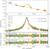 |
Fig. 1 Light curve of the microlensing event MOA-2022-BLG-249. The arrow marked by tanom in the second panel indicates the location of the anomaly. Top panel shows the enlarged view around the anomaly region. The solid and dashed curves drawn over the data points are 1L1S models obtained with (parallax model) and without (standard model) the consideration of microlens-parallax effects. Two lower panels shows the residuals from the two models. |
3 Light curve analysis
It is known that a brief positive anomaly in a lensing light curve can arise via two channels: one by a low-mass companion to the lens (Mao & Paczyński 1991; Gould & Loeb 1992) and the other by a faint companion to the source (Gaudi 1998). In this section, we present the analysis of the lensing light curve conducted to reveal the nature of the anomaly. Details of the analysis based on the single-lens binary-source (1L2S) and the binary-lens and single-source (2L1S) interpretations are presented in Sects. 3.1 and 3.2, respectively.
The analysis under each interpretation was carried out in search for a lensing solution, which represents a set of lensing parameters describing the observed lensing light curve. The common lensing parameters for both 2L1S and 1L2S models are (t0, u0, tE, ρ), which represent the time of the closest lens-source approach, the projected lens-source separation scaled to the angular Einstein radius (θE) at t0 (impact parameter), the event time scale, and the source radius scaled to θE (normalized source radius), respectively. Besides these basic parameters, a 2L1S modeling requires extra parameters of (s, q, α), where the first two parameters represent the projected separation (scaled to θE) and mass ratio between the lens components, respectively, and the last parameter denotes the angle of the source trajectory as measured from the binary-lens axis. A 1L2S model also requires additional parameters, including (t0,2, u0,2, ρ2, qF), which represent the closest approach time, impact parameter and the normalized radius of the secondary source, and the flux ratio between the secondary and primary source stars, respectively. In the 1L2S model, we designate the time of closest approach, the impact parameter and normalized radius of the primary source as t0,1, u0,1and ρ1, respectively, to distinguish them from those describing the secondary source.
In the modeling, we take the microlens-parallax effects into consideration because the event lasted for a significant fraction of a year. For a long time-scale event like MOA-2022-BLG-249, the deviation of the source motion from rectilinear caused by the orbital motion of Earth around the sun can be substantial (Gould 1992). In order to consider these effects in the modeling, we add two extra lensing parameters (πE,N, πE,E), which denote the north and east components of the microlens-lens parallax vector πE = (πrel/θE)(µ/µ), respectively. Here, µ represents the vector of the relative lens-source proper motion and πrel denotes the relative lens-source parallax, which is related to the distance to the lens, DL, and source, DS, by πrel = AU(1/DL – 1/DS). In each parallax modeling, we checked a pair of solutions with u0 > 0 and u0 < 0.
1L2S model parameters.
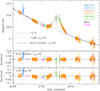 |
Fig. 2 Comparison of the 2L1S and 1L2S models. Lower two panels show the residuals from the individual models. |
3.1 1L2S model
The 1L2S modeling was carried via a downhill approach using the Markov chain Monte Carlo (MCMC) method because the lensing magnification smoothly changes with the variation of the 1L2S lensing parameters. The initial parameters of (t0, u0, tE) were given by adopting the values obtained from the 1L1S modeling, while those related to the source companion, that is, (t0,2, u0,2, ρ2, qF), were given by considering the location and magnitude of the anomaly. We refer to Hwang et al. (2013) for details of the 1L2S modeling. The lensing parameters of the u0 > 0 and u0 < 0 solutions and their χ2 values of the fit together with the degree of freedom (d.o.f.) are listed in Table 2. It is found that the solution with u0,1 < 0 results in a slightly better fit than the solution with u0,1 > 0, by ∆χ2 = 1.6. The model curve of the u0,1 < 0 solution and its residual in the region of the anomaly are shown in Fig. 2. It is found that the 1L2S models approximately delineate the observed anomaly, but they leave slight residual both in the rising and falling parts of the anomaly. In particular, the negative residuals in the rising part of the anomaly appears both in the KMTS and CFHT data sets, suggesting that these residuals are likely to be real.
The lens-system configuration of the u0,1 < 0 model is shown in the bottom panel of Fig. 3, in which the arrowed curves marked in blue and red represent the trajectories of the primary (labeled as “S1”) and secondary source (labeled as “S2”) stars, respectively. According to the 1L2S interpretation, the anomaly was produced by the close approach of a secondary source to the lens. The secondary source is very faint, and its flux is ~0.5% of the flux from the primary source.
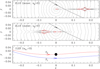 |
Fig. 3 Lens system configurations. Two upper panels show the configurations of the inner and outer 2L1S solutions with u0 > 0 and the bottom panel shows the configuration of the 1L2S solution with u0,1 < 0. In each of the panels showing the 2L1S configurations, the red cuspy figures represent caustics, the line with an arrow is the source trajectory, and grey curves encompassing the caustic are equi-magnification contours. In the panel of the 1L2S solution, the black filled dot represent the lens, and the blue and red curves denote the trajectories of the primary (marked by S1) and secondary (marked by S1) source stars, respectively. |
3.2 2L1S model
The 2L1S modeling was conducted in two steps. In the first step, we searched for the binary-lens parameters s and q via a grid approach with multiple starting values of the source trajectory angle α, while we found the other lensing parameters via a downhill approach. We then constructed a ∆χ2 map on the (s, q) parameter plane and identified a pair of degenerate solutions resulting from the “inner-outer” degeneracy (Gaudi & Gould 1997). In the second step, we refined the lensing parameters of the individual local solutions by allowing all parameters to vary.
In Table 3, we list the lensing parameters of the inner and outer 2L1S solutions, for each of which there are a pair of solutions with u0 > 0 and u0 < 0. Among the solutions, it was found that the inner solution with u0 > 0 yields the best fit to the data. From the comparison of the 2L1S fit with that of 1L2S fit, it is found that the anomaly is better explained by the 2L1S interpretation than the 1L2S interpretation. In Fig. 2, we draw the model curve of the inner 2L1S solution (with u0 > 0) and its residual, showing that the residual of the 1L2S model around the anomaly does not appear in the residual of the 2L1S model. From a comparison of the fits, it is found that the 2L1S model provides a better fit to the data than the 1L2S model by ∆χ2 = 181.2, indicating that the origin of the perturbation is a low-mass companion to the lens rather than a faint companion to the source.
The lens-system configurations of the inner and outer 2L1S solutions, with u0 > 0 values, are shown in the two upper panels of Fig. 3. According to the inner and outer solutions, the anomaly was produced by the source passages through the regions lying on the side close to and farther from the planetary caustic, respectively. The inner and outer solutions can be viewed as “wide” and “close” solutions, respectively, arising due to the similarity between the central caustics induced by a wide planet and a close planet: a “close-wide” degeneracy (Griest & Safizadeh 1998). Yee et al. (2021) pointed out that the transition between the outer-inner and close-wide degeneracies is continuous, and Hwang et al. (2022) introduced an analytic expression for the relation between the binary separations of the inner (sin) and outer (sout) solutions:
 (1)
(1)
Here  represents the lens-source separation at the time of the anomaly, tanom, and τanom = (tanom − t0)/tE. It is found that the value of s† estimated from the planet separations (sin, sout) = (1.086, 0.967), that is, s† = (sin × sout)1/2 = 1.024, matches the value estimated from the lensing parameters (t0, u0, tE, tanom) very well, that is,
 ![Mathematical equation: ${s^\dag } = {{\left[ {{{\left( {u_{{\rm{anom}}}^2 + 4} \right)}^{{1 \mathord{\left/ {\vphantom {1 2}} \right. \kern-\nulldelimiterspace} 2}}} + {u_{{\rm{anom}}}}} \right]} \mathord{\left/ {\vphantom {{\left[ {{{\left( {u_{{\rm{anom}}}^2 + 4} \right)}^{{1 \mathord{\left/ {\vphantom {1 2}} \right. \kern-\nulldelimiterspace} 2}}} + {u_{{\rm{anom}}}}} \right]} {2 = 1.024}}} \right. \kern-\nulldelimiterspace} {2 = 1.024}}$](/articles/aa/full_html/2023/06/aa46166-23/aa46166-23-eq3.png) . The estimated companion-to-primary mass ratio, q ~ 8 × 10⁻⁵, is very low for both the inner and outer solutions, while the event time scale, tE ~ 134 days, is substantially longer than the several weeks of typical Galactic lensing events (Han & Gould 2003). The normalized source radius cannot be accurately measured because the source did not cross the caustic and only the upper limit, ρmax = 1.2 × 10⁻³, can be placed. See the scatter plot of the MCMC points on the (u0, ρ) parameter plane presented in Fig. 4.
. The estimated companion-to-primary mass ratio, q ~ 8 × 10⁻⁵, is very low for both the inner and outer solutions, while the event time scale, tE ~ 134 days, is substantially longer than the several weeks of typical Galactic lensing events (Han & Gould 2003). The normalized source radius cannot be accurately measured because the source did not cross the caustic and only the upper limit, ρmax = 1.2 × 10⁻³, can be placed. See the scatter plot of the MCMC points on the (u0, ρ) parameter plane presented in Fig. 4.
We note that the degeneracy between the 2L1S and 1L2S models was able to be securely resolved thanks to the nature of the event with a high peak magnification and an acute source trajectory angle. In this case, the duration of the anomaly increases by a factor |1/ sin α| (Yee et al. 2021), which corresponds to a factor of 2.1 in the case of MOA-2022-BLG-249. That is to say, if this anomaly occurred with a right angle, that is, α ~ 90° or 270°, then the anomaly would have been half as short and the data might not have been good enough to distinguish the 2L1S model from the 1L2S model. For events with acute trajectory angles, the magnification is lower than the peak magnification by a factor | sin α|. This factor is 0.47 (0.8 magnitudes) in the case of MOA-2022-BLG-249.
Parameters of 2L1S models (parallax only).
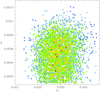 |
Fig. 4 Scatter plot of points in the MCMC chain on the (u0, ρ) parameter plane obtained from the 2L1S modeling. The color coding is set to designate points with ≤1σ (red), ≤2σ (yellow), ≤3σ (green), ≤4σ (cyan), and ≤5σ (blue). |
3.3 Microlens-parallax effects
It has been found that considering parallax effects is important for the precise description of the observed light curve. This is somewhat expected from the long time scale of the event. The improvement of the fit with the parallax effect is huge, that is, by ∆χ2 = 5300 with respect to the model obtained under the assumption that the relative lens-source motion is rectilinear. The inner and outer 2L1S solutions result in similar values of the parallax parameters of (πE,N, πE,E) ~ (−0.48, 0.27).
We checked the solidness of the parallax measurement by inspecting the consistency of the parallax parameters measured from the 1L1S and 2L1S modeling. Figure 5 shows the scatter plots of MCMC points of the 1L1S solution and the inner and outer 2L1S solutions with positive u0 values. The parallax modeling was conducted by excluding the data around the perturbation (9730 < HJD′ < 9736) because the parallactic Earth motion has a long-term effect on the lensing light curve. From this check, it was found that all the tested models result in consistent parallax parameters and this indicates that the parallax parameters are securely measured.
We also checked the effect of the planetary orbital motion on the πE measurement because the planet might have moved during the 6-day period between the peak and the planetary perturbation and this could affect the lens system configuration. For this check, we tested additional models considering the planetary motion by including two orbital parameters of (ds/dt, dα/dt), which represent the annual change rates of the planetary separation and source trajectory angle, respectively. The lensing parameters of the solutions considering the lens-orbital motion are listed in Table 4. It is found that the lens-orbital motion does not have a significant effect on the microlens-parallax parameters. This can be seen in Fig. 6, where we present the scatter plots of the MCMC points on the (πE,N,πE,E,ds/dt,dα/dt) parameter planes for the inner u0 > 0 solution, considering both the microlens-parallax and lens-orbital effects. The plots show that the uncertainties of the orbital parameters, that is, ds/dt and dα/dt, are very large. Although there are some variations of the plots in the orbital-parameter space for the other solutions, that is, the inner solution with u0 < 0 and outer solutions with u0 > 0 and u0 < 0, the variation of the parallax parameters is minor. Furthermore, the parallax parameters are similar to the values determined without considering the lens-orbital effect. These results indicate that the effect of the lens-orbital motion on the light curve is minor.
We additionally checked the possibility that the parallax effect is imitated by the orbital effect induced by a source companion for which its luminosity contribution to the lensing light curve is negligible: xallarap effects (Griest & Hu 1992; Han & Gould 1997; Smith et al. 2002). For this check, we conducted an additional modeling with the consideration of xallarap effects. Following the parameterization of Dong et al. (2009), the xal-larap modeling was done by including five extra parameters of (ξE,N,ξE,E,P,ψ,i). Here the first two parameters (ξE,N,ξE,E) denote the north and east components of the xallarap vector, ξE, respectively, and the other parameters represent the period, phase angle, and inclination of the binary-source orbit, respectively. The magnitude of the xallarap vector,  , is related to the semi-major axis, a, of the source orbit by
  , where
  denotes the physical Einstein radius projected onto the source plane, aS = aMS,2/(MS,1 + MS,2), and (MS,1,MS,2) are the masses of source components. Combined with the Kepler’s law, the mass ratio between the source stars, Q = MS,2/MS,1, follows the relation (Dong et al. 2009)
 (2)
(2)
The result of the xallarap modeling is presented in Fig. 7, in which the left and right panels show χ2 value of the xallarap fit and the lower limit of R = Q3/(1 + Q)2 value with respect to the orbital period of the source, respectively. For the computation of R, we adopted the mass of the primary source of MS,1 ~ 1 M⊙ and distance to the source of DS = 8 kpc. For the angular Einstein radius, we adopted the lower limit of θE,min ~ 0.46 mas because R ∝ aS ∝ θE, and thus the lower limit of the R value results from the lower limit of θE. The procedure of θE,min determination is discussed in Sect. 4. From the comparison of the χ2 values between the xallarap,  , and parallax,
  , solutions, it is found that
  is higher than
  for solutions with P < 1 yr, almost same as
  for solutions with P ~ 1 yr, and slightly lower than
  for solutions with P > 1 yr. For the solutions with P > 1 yr, the χ2 difference
  is very minor with three additional dof, and this corresponds to about 11% probability even assuming Gaussian statistics. Furthermore, the ratio R ≳ 40 for these solutions and, thus, the mass ratio ratio is Q ≳ 40, implying that mass of the source companion is MS,2 ~ 40 M⊙, which corresponds to that of a black hole and thus unphysical. The results of the xallarap models indicate that there is no evidence that the light curve is affected by xallarap effects and, more importantly, no evidence that the parallax signal is actually due to systematics. Therefore, we conclude that the parallax signal is real. As discussed in Sect. 4, the source may be a disk star lying in front of the bulge and the source distance may be smaller than the adopted value of 8 kpc, but this has little impact on the conclusions resulting from the xallarap modeling.
Parameters of 2L1S models (orbit+parallax).
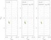 |
Fig. 5 Scatter plots of the MCMC points in the chains of the 1L1S, and the inner and outer 2L1S solutions on the (πE,E,πE,N) parameter plane. In all cases, we present plots of the solutions with u0 > 0, while the solutions with u0 < 0 result in similar plots. The dotted circles are drawn at every 0.2πE interval. The color coding is same as that used in Fig. 4. |
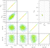 |
Fig. 6 Scatter plot of the MCMC chain on the parameter planes of higher-order parameters of (πE,N,πE,E, ds/dt, dα/dt) for the inner 2L1S solution with u0 > 0 obtained considering both microlens-parallax and lens-orbital effects. The plot on the (πE,E, πE,N) plane in the upper right inset is presented for the direct comparison with the plots presented in Fig. 5. |
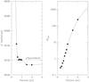 |
Fig. 7 Results of the xallarap modeling. Left panel shows the χ2 values of the xallarap fits as a function of the source orbital period and the right panel shows the lower limit of R = Q3/(1 + Q)2 as a function of the period. The dashed horizontal line in the left panel indicates the χ2 value of the parallax fit. |
4 Source star and Einstein radius
In this section, we define the source star of the lensing event not only for the purpose of fully characterizing the event, but also for constraining the lensing observable of the angular Einstein radius. The value of θE is estimated from the normalized source radius and angular source radius θ*, by θE = θ*,/ρ. Although the ρ value cannot be measured for MOA-2022-BLG-249 due to the non-caustic-crossing nature of the anomaly, it is possible to constrain its upper limit, which yields the lower limit of the Einstein radius, that is, θE,min = θ*/ρmax.
We specified the type of the source star by measuring its color and magnitude. For this specification, we first placed the source in the instrumental color-magnitude diagram (CMD) of stars around the source by measuring the V- and I-band magnitudes of the source by regressing the light curve data measured in the individual passbands with respect to the lensing magnification estimated by the model. We then calibrated the source color and magnitude using the centroid of the red giant clump (RGC), for which its extinction-corrected (de-reddened) color and magnitude are known, as a reference (Yoo et al. 2004), that is,
![Mathematical equation: ${\left( {V - I,I} \right)_{0,{\rm{S}}}} = {\left( {V - I,I} \right)_{0{\rm{,RGC}}}} + \left[ {{{\left( {V - I,I} \right)}_{\rm{S}}} - {{\left( {V - I,I} \right)}_{{\rm{RGC}}}}} \right].$](/articles/aa/full_html/2023/06/aa46166-23/aa46166-23-eq15.png) (3)
(3)
Here, (V – I, I)S and (V – I, I)rgc denote the instrumental colors and magnitudes of the source and RGC centroid, respectively, and (V – I, I)0,S and (V – I, I)0,RGC indicate their corresponding de-reddened values.
Figure 8 shows the locations of the source and RGC centroid in the instrumental CMD. We also marked the location of the blend. The instrumental color and magnitude are (V – I, I)S = (2.785 ± 0.017, 20.700 ± 0.001) for the source and (V – I, I)rgc = (3.285, 16.800) for the RGC centroid. With the known de-reddened color and magnitude of the RGC centroid, (V – I, I)0,rgc = (1.060, 14.530) (Bensby et al. 2013; Nataf et al. 2013), we estimated the de-reddened color and magnitude of the source of:
 (4)
(4)
According to the estimated color and magnitude, the source is a mid to late F-type main-sequence star and it probably lies in the disk in front of the bulge, although it could be a rare star in the bulge.
We also estimated the de-reddened color and brightness of the blend as (V – I, I)0,b = (0.76, 19.31), assuming that the blend lies behind most of the dust, that is, in or near the bulge. We checked the possibility that the lens is the major source of the blended flux. For this check, we measured the astrometric offset between the centroids of the source measured before and at the time of the lensing magnification. Considering that this offset is measured in the same season, it is expected that the offset would be smaller than the measurement uncertainty if the lens is the blend. The measured offset in the KMTC image is Δθ = (169.2 ± 44.7) mas. This 3.8σ offset is confirmed by the offset Δθ = (80 ± 10) mas measured in the CFHT data taken with seeing of 0.45′′–0.55′′. This indicates that the blend is caused by a nearby star lying close to the source rather than the lens.
With the specification of the source, we then estimate the angular radius of the source. For this, we first converted the measured V – I color into V – K color with the use of the Bessell & Brett (1988) relation and then estimated the angular radius of the source using the (V – K, V)–θ*, relation of Kervella et al. (2004). We estimated that the source has an angular radius of:
 (5)
(5)
and this yields the minimum values of the angular Einstein radius:
 (6)
(6)
and the relative lens-source proper motion:
 (7)
(7)
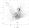 |
Fig. 8 Source location with respect to the red giant clump (RGC) in the instrumental CMD. The location of the blend is marked. |
5 Physical lens parameters
The physical parameters of a lens are constrained by measuring the lensing observables of an event. These observables include the event time scale, tE, Einstein radius, θE, and microlens parallax vector, πE = (πE,N,πE,E), and the mass and distance to the lens are determined from the combination of these observables as
 (8)
(8)
respectively (Gould 2000). Here κ = 4G/(c2AU) and πS = AU/DS is the parallax of the source. For MOA-2022-BLG-249, the values of tE and πE are securely measured, but the value of θE cannot be measured and only its lower limit is constrained, making it difficult to analytically estimate M and DL using the relations in Eq. (8). We, therefore, estimate the physical lens parameters by conducting a Bayesian analysis based on the measured lensing observables and other available constraints.
In the first step of the Bayesian analysis, we generated a large number (2 × 10⁸) of artificial lensing events, for which the locations the lens and source and their relative proper motion were assigned on the basis of a Galactic model and the lens masses were allocated on the basis of a mass-function model by conducting a Monte Carlo simulation. In the simulation, we adopted the models of the Galaxy and lens mass function described in Jung et al. (2021) and Jung et al. (2018), respectively. For each simulated event, we computed the lensing observables corresponding to the values of M, DL, DS, and µ by
 (9)
(9)
In the second step, we imposed a weight wi = exp(−χ2/2) to each artificial event and constructed posteriors of M and DL. In this procedure, the χ2 value is calculated as
 (10)
(10)
where (πE,1,πE,2)i = (πE,N,πE,E)i is expressed in two component form, (tE,i, πE,i) are the observables of each simulated event, (tE, πE) represent the measured observables,  , is the uncertainty in the tE measurement, and bjk is the inverse covariance matrix of πE. We refer to Eqs. (10) and (11) of Gould et al. (2022). Finally, we imposed the constraint of the Einstein radius by setting wi = 0 for events with θE ≤ θE,min.
We imposed an additional constraint provided by the fact that the flux from the lens cannot be greater than the blend flux. Imposing this blend-flux constraint may be important because the distance to the lens expected from the large value of the measured microlens parallax,  , is small. In order to impose this constraint, we computed the lens magnitude as:
 (11)
(11)
where MI,L is the absolute I-band magnitude of a star corresponding to the lens mass, and AI,L represents the I-band extinction to the lens. For the computation of AI,L, we modeled the extinction as
![Mathematical equation: ${A_{I,{\rm{L}}}} = {A_{I,{\rm{tot}}}}\,\left[ {1 - \exp \,\left( { - {{\left| z \right|} \over {{h_{z,{\rm{dust}}}}}}} \right)} \right],$](/articles/aa/full_html/2023/06/aa46166-23/aa46166-23-eq26.png) (12)
(12)
where AI,tot = 2.49 is the total I-band extinction toward the field, hz,dust = 100 pc is the vertical scale height of dust, z = DL sin b + z0, b is the Galactic latitude, and z0 = 15 pc is vertical position of the Sun above the Galactic plane.
Figure 9 shows the Bayesian posteriors of the host mass (top panel), Mhost, distances to the planetary system (middle panel), and source (bottom panel). We present two sets of posterior: one with (shaded distribution) and the other without (unshaded distribution) the blend-flux constraint. The posterior distributions show that the physical parameters are tightly defined despite the limited information on the angular Einstein radius. In Table 5, we summarize the estimated physical parameters, in which the median values are presented as representative values and the uncertainties are estimated as 16% and 84% of the Bayesian posterior distributions. Here, the planet mass is estimated as Mplanet = qMhost and the projected planet-host separation is computed by a⊥ = SθEDL. From the fact that the lower mass limit and the upper distance limit estimated using the analytic relations in Eq. (8) based on the lower limit of the Einstein radius, that is, Mmin = θE,min/κπE ~ 0.12 M⊙ and DL,max = AU/(πEθE,min + πS) ~ 2.4 kpc, match well the corresponding limits of the Bayesian posteriors indicates that these limits of the physical parameters are set by the combination of the constraints provided by θE,min and πE. On the other hand, the upper limit of the mass and lower limit of the distance are set by the blend-flux constraint. This can be seen from the comparison of the Bayesian posteriors obtained, with and without imposing the lens flux constraint.
It turns out that the lens is a planetary system, in which a low-mass planet orbits a low-mass host star lying in the Galactic disk. The estimated mass of the planet, Mplanet ~ 4.8 M⊕, indicates that the planet is a super-Earth, and the detection of the system aptly demonstrates the elevated microlensing sensitivity to low-mass planets with the increase of the observational cadence. The estimated mass of the host, Mhost ~ 0.18 M⊙, and distance, DL ~ 2.0 kpc, indicate that the host of the planet is a very low-mass M dwarf lying in the Galactic disk. Finding planets belonging to such low-mass stars using other methods is difficult because of the faintness of host stars, and thus the discovered planetary system well demonstrates the usefulness of the microlensing method in finding planets with low-mass host stars. The planetary system lies at a substantially closer distance than those of typical microlensing planets, which usually lie either in the bulge or in the portion of the disk that is closer to the bulge than to the Sun. We checked the hypothesis that the source is in the disk by additionally conducting a Bayesian analysis, in which we assumed that DS = 7 kpc and the dispersion of the source motion is negligible, as in the case of disk stars. We found that this analysis results in similar posteriors to those presented in Fig. 9, indicating that the uncertain source location has little effect on the result.
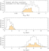 |
Fig. 9 Bayesian posteriors of the lens mass, distance to the lens and source. In each panel, the shaded and and unshaded distributions are obtained with (shaded) and without (unshaded) imposing the blend-flux constraint, respectively. |
Physical lens parameters.
6 Summary and conclusion
We analyzed the microlensing event MOA-2022-BLG-249, for which the light curve exhibits a brief positive anomaly with a duration of ~ 1 day and a maximum deviation of ~0.2 mag from a single-source single-lens model. We tested both the planetary and binary-source origins, which are the two channels producing a short-term positive anomaly in a lensing light curve.
We found that the anomaly was produced by a planetary companion to the lens, rather than a binary companion to the source. We identified two solutions rooted in the inner-outer degeneracy, for both of which the estimated planet-to-host mass ratio, q ~ 8 × 10⁻⁵, is very small. With the constraints provided by the microlens parallax, along with the lower limit of the Einstein radius taken together with the blend-flux constraint, we find that the lens is a planetary system, in which a super-Earth planet, with a mass of (4.83 ± 1.44) M⊕, orbits a low-mass host star, with a mass of (0.18 ± 0.05) M⊙, lying in the Galactic disk at a distance (2.00 ± 0.42) kpc. The planet detection aptly demonstrates the elevated microlensing sensitivity of the current high-cadence lensing surveys to low-mass planets.
Acknowledgements
Work by C.H. was supported by the grants of National Research Foundation of Korea (2020R1A4A2002885 and 2019R1A2C2085965). This research has made use of the KMTNet system operated by the Korea Astronomy and Space Science Institute (KASI) and the data were obtained at three host sites of CTIO in Chile, SAAO in South Africa, and SSO in Australia. This research was supported by the Korea Astronomy and Space Science Institute under the R&D program (Project No. 2023-1-832-03) supervised by the Ministry of Science and ICT. The MOA project is supported by JSPS KaKENHI Grant Number JSPS24253004, JSPS26247023, JSPS23340064, JSPS15H00781, JP16H06287, and JP17H02871. J.C.Y., I.G.S., and S.J.C. acknowledge support from NSF Grant No. AST-2108414. Y.S. acknowledges support from NSF Grant No. 2020740. This research uses data obtained through the Telescope Access Program (TAP), which has been funded by the TAP member institutes. W. Zang, H.Y., S.M., and W. Zhu acknowledge support by the National Science Foundation of China (Grant No. 12133005). W. Zang acknowledges the support from the Harvard-Smithsonian Center for Astrophysics through the CfA Fellowship. W. Zhu acknowledges the science research grants from the China Manned Space Project with No. CMS-CSST-2021-A11. C.R. was supported by the Research fellowship of the Alexander von Humboldt Foundation.
References
- Beaulieu, J.-P., Bennett, D. P., Fouqué, P., et al. 2006, Nature, 439, 437 [Google Scholar]
- Bennett, D. P., & Rhie, S. H. 1996, ApJ, 472, 660 [NASA ADS] [CrossRef] [Google Scholar]
- Bennett, D. P., Bond, I. A., Udalski, A., et al. 2008, ApJ, 684, 663 [Google Scholar]
- Bennett, D. P., Batista, V., Bond, I. A., et al. 2014, ApJ, 785, 155 [Google Scholar]
- Bensby, T. Yee, J.C., Feltzing, S., et al. 2013, A & A, 549, A147 [NASA ADS] [CrossRef] [EDP Sciences] [Google Scholar]
- Bessell, M. S., & Brett, J. M. 1988, PASP, 100, 1134 [Google Scholar]
- Bond, I. A., Abe, F., Dodd, R. J., et al. 2001, MNRAS, 327, 868 [Google Scholar]
- Bond, I. A., Bennett, D. P., Sumi, T., et al. 2017, MNRAS, 469, 2434 [Google Scholar]
- Dong, S., Gould, A., Udalski, A., et al. 2009, ApJ, 695, 970 [NASA ADS] [CrossRef] [Google Scholar]
- Gaudi, B. S. 1998, ApJ, 506, 533 [Google Scholar]
- Gaudi, B. S. 2012, ARA & A, 50, 411 [NASA ADS] [CrossRef] [Google Scholar]
- Gaudi, B. S., & Gould, A. 1997, ApJ, 486, 85 [Google Scholar]
- Gaudi, B. S., & Han, C. 2004, ApJ, 611, 528 [NASA ADS] [CrossRef] [Google Scholar]
- Gould, A. 1992, ApJ, 392, 442 [Google Scholar]
- Gould, A. 2000, ApJ, 542, 785 [NASA ADS] [CrossRef] [Google Scholar]
- Gould, A., & Loeb, A. 1992, ApJ, 396, 104 [Google Scholar]
- Gould, A., Udalski, A., Shin, I.-G., et al. 2014, Science, 345, 46 [Google Scholar]
- Gould, A., Ryu, Y.-H., Calchi Novati, S., et al. 2020, JKAS, 53, 9 [NASA ADS] [Google Scholar]
- Gould, A., Han, C., Weicheng, Z., et al. 2022, A & A, 664, A13 [NASA ADS] [CrossRef] [EDP Sciences] [Google Scholar]
- Griest, K., & Hu, W. 1992, ApJ, 397, 362 [Google Scholar]
- Griest, K., & Safizadeh, N. 1998, ApJ, 500, 37 [Google Scholar]
- Han, C. 2006, ApJ, 638, 1080 [Google Scholar]
- Han, C., & Gould, A. 1997, ApJ, 480, 196 [NASA ADS] [CrossRef] [Google Scholar]
- Han, C., & Gould, A. 2003, ApJ, 502, 172 [NASA ADS] [CrossRef] [Google Scholar]
- Han, C., Hirao, Y., Udalski, A., et al. 2018, AJ, 155, 211 [NASA ADS] [CrossRef] [Google Scholar]
- Han, C., Udalski, A., Lee, C.-U., et al. 2021, A & A, 649, A90 [NASA ADS] [CrossRef] [EDP Sciences] [Google Scholar]
- Han, C., Bond, I. A., Yee, J. C., et al. 2022a, A & A, 658, A94 [NASA ADS] [CrossRef] [EDP Sciences] [Google Scholar]
- Han, C., Gould, A., Albrow, M. D., et al. 2022b, A & A, 658, A62 [NASA ADS] [CrossRef] [EDP Sciences] [Google Scholar]
- Herrera-Martin, A., Albrow, M. D., Udalski, A., et al. 2020, AJ, 159, 256 [NASA ADS] [CrossRef] [Google Scholar]
- Hwang, K.-H., Choi, J.-Y., Bond, I. A., et al. 2013, ApJ, 778, 55 [Google Scholar]
- Hwang, K.-H., Zang, W., Gould, A., et al. 2022, AJ, 163, 43 [NASA ADS] [CrossRef] [Google Scholar]
- Jung, Y. K., Udalski, A., Gould, A., et al. 2018, AJ, 155, 219 [Google Scholar]
- Jung, Y. K., Han, C., Udalski, A., et al. 2021, AJ, 161, 293 [NASA ADS] [CrossRef] [Google Scholar]
- Kervella, P., Thévenin, F., Di Folco, E., & Ségransan, D. 2004, A & A, 426, 29 [Google Scholar]
- Kim, S.-L., Lee, C.-U., Park, B.-G., et al. 2016, JKAS, 49, 37 [Google Scholar]
- Kondo, I., Yee, J. C., Bennett, D. P., et al. 2021, AJ, 162, 77 [NASA ADS] [CrossRef] [Google Scholar]
- Mao, S., & Paczynski, B. 1991, ApJ, 374, 37 [Google Scholar]
- Mróz, P., Poleski, R., Gould, A., et al. 2020, ApJ, 903, L11 [Google Scholar]
- Muraki, Y., Han, C., Bennett, D. P., et al. 2011, ApJ, 741, 22 [Google Scholar]
- Nataf, D. M., Gould, A., Fouqué, P., et al. 2013, ApJ, 769, 88 [Google Scholar]
- Ryu, Y.-H., Udalski, A., Yee, J. C., et al. 2020, AJ, 160, 183 [Google Scholar]
- Ryu, Y.-H., Jung, Y. K., Yang, H., et al. 2022, AJ, 164, 180 [CrossRef] [Google Scholar]
- Shvartzvald, Y., Yee, J. C., Calchi Novati, S., et al. 2017, ApJ, 840, L3 [Google Scholar]
- Smith, M. C., Mao, S., Wozniak, P., et al. 2002, MNRAS, 336, 670 [NASA ADS] [CrossRef] [Google Scholar]
- Sumi, T., Udalski, A., Bennett, D. P., et al. 2016, ApJ, 825, 112 [Google Scholar]
- Udalski, A., Szymanski, M. K., & Szymanski, G. 2015, Acta Astron., 65, 1 [Google Scholar]
- Yee, J. C., Shvartzvald, Y., Gal-Yam, A., et al. 2012, ApJ, 755, 102 [Google Scholar]
- Yee, J. C., Zang, W., Udalski, A., et al. 2021, AJ, 162, 180 [NASA ADS] [CrossRef] [Google Scholar]
- Yoo, J., DePoy, D. L., Gal-Yam, A., et al. 2004, ApJ, 603, 139 [Google Scholar]
- Vandorou, A., Dang, L., Bennett, D. P., et al. 2023, AJ, submitted [arXiv:2302.01168] [Google Scholar]
- Zang, W., Han, C., Kondo, I., et al. 2021a, RAA, 21, 239 [NASA ADS] [Google Scholar]
- Zang, W., Hwang, K.-H., Udalski, A., et al. 2021b, AJ, 162, 163 [NASA ADS] [CrossRef] [Google Scholar]
- Zang, W., Jung, Y. K., Yang, H., et al. 2023, AJ, 165, 103 [CrossRef] [Google Scholar]
All Tables
All Figures
|
Fig. 1 Light curve of the microlensing event MOA-2022-BLG-249. The arrow marked by tanom in the second panel indicates the location of the anomaly. Top panel shows the enlarged view around the anomaly region. The solid and dashed curves drawn over the data points are 1L1S models obtained with (parallax model) and without (standard model) the consideration of microlens-parallax effects. Two lower panels shows the residuals from the two models. |
| In the text | |
|
Fig. 2 Comparison of the 2L1S and 1L2S models. Lower two panels show the residuals from the individual models. |
| In the text | |
|
Fig. 3 Lens system configurations. Two upper panels show the configurations of the inner and outer 2L1S solutions with u0 > 0 and the bottom panel shows the configuration of the 1L2S solution with u0,1 < 0. In each of the panels showing the 2L1S configurations, the red cuspy figures represent caustics, the line with an arrow is the source trajectory, and grey curves encompassing the caustic are equi-magnification contours. In the panel of the 1L2S solution, the black filled dot represent the lens, and the blue and red curves denote the trajectories of the primary (marked by S1) and secondary (marked by S1) source stars, respectively. |
| In the text | |
|
Fig. 4 Scatter plot of points in the MCMC chain on the (u0, ρ) parameter plane obtained from the 2L1S modeling. The color coding is set to designate points with ≤1σ (red), ≤2σ (yellow), ≤3σ (green), ≤4σ (cyan), and ≤5σ (blue). |
| In the text | |
|
Fig. 5 Scatter plots of the MCMC points in the chains of the 1L1S, and the inner and outer 2L1S solutions on the (πE,E,πE,N) parameter plane. In all cases, we present plots of the solutions with u0 > 0, while the solutions with u0 < 0 result in similar plots. The dotted circles are drawn at every 0.2πE interval. The color coding is same as that used in Fig. 4. |
| In the text | |
|
Fig. 6 Scatter plot of the MCMC chain on the parameter planes of higher-order parameters of (πE,N,πE,E, ds/dt, dα/dt) for the inner 2L1S solution with u0 > 0 obtained considering both microlens-parallax and lens-orbital effects. The plot on the (πE,E, πE,N) plane in the upper right inset is presented for the direct comparison with the plots presented in Fig. 5. |
| In the text | |
|
Fig. 7 Results of the xallarap modeling. Left panel shows the χ2 values of the xallarap fits as a function of the source orbital period and the right panel shows the lower limit of R = Q3/(1 + Q)2 as a function of the period. The dashed horizontal line in the left panel indicates the χ2 value of the parallax fit. |
| In the text | |
|
Fig. 8 Source location with respect to the red giant clump (RGC) in the instrumental CMD. The location of the blend is marked. |
| In the text | |
|
Fig. 9 Bayesian posteriors of the lens mass, distance to the lens and source. In each panel, the shaded and and unshaded distributions are obtained with (shaded) and without (unshaded) imposing the blend-flux constraint, respectively. |
| In the text | |
Current usage metrics show cumulative count of Article Views (full-text article views including HTML views, PDF and ePub downloads, according to the available data) and Abstracts Views on Vision4Press platform.
Data correspond to usage on the plateform after 2015. The current usage metrics is available 48-96 hours after online publication and is updated daily on week days.
Initial download of the metrics may take a while.