| Issue |
A&A
Volume 664, August 2022
|
|
|---|---|---|
| Article Number | A114 | |
| Number of page(s) | 10 | |
| Section | Planets and planetary systems | |
| DOI | https://doi.org/10.1051/0004-6361/202243161 | |
| Published online | 17 August 2022 | |
KMT-2021-BLG-0240: Microlensing event with a deformed planetary signal
1
Department of Physics, Chungbuk National University,
Cheongju
28644, Republic of Korea
e-mail: cheongho@astroph.chungbuk.ac.kr
2
Department of Astronomy, Tsinghua University,
Beijing
100084, PR China
3
Max Planck Institute for Astronomy,
Königstuhl 17,
69117
Heidelberg, Germany
4
Department of Astronomy, The Ohio State University,
140 W. 18th Ave.,
Columbus, OH
43210, USA
5
Korea Astronomy and Space Science Institute,
34055
Daejon, Republic of Korea
6
University of Canterbury, Department of Physics and Astronomy,
Private Bag 4800,
Christchurch
8020, New Zealand
7
Department of Particle Physics and Astrophysics, Weizmann Institute of Science,
Rehovot
76100, Israel
8
Center for Astrophysics, Harvard & Smithsonian,
60 Garden St.,
Cambridge, MA
02138, USA
9
School of Space Research, Kyung Hee University,
Yongin, Kyeonggi
17104, Republic of Korea
Received:
19
January
2022
Accepted:
20
April
2022
Aims. The light curve of the microlensing event KMT-2021-BLG-0240 exhibits a short-lasting anomaly with complex features near the peak at the 0.1 mag level from a single-lens single-source model. We conducted modeling of the lensing light curve under various interpretations to reveal the nature of the anomaly.
Methods. It is found that the anomaly cannot be explained with the usual model based on a binary-lens (2L1S) or a binary-source (1L2S) interpretation. However, a 2L1S model with a planet companion can describe part of the anomaly, suggesting that the anomaly may be deformed by a tertiary lens component or a close companion to the source. From the additional modeling, we find that all the features of the anomaly can be explained with either a triple-lens (3L1S) model or a binary-lens binary-source (2L2S) model. However, it is difficult to validate the 2L2S model because the light curve does not exhibit signatures induced by the source orbital motion and the ellipsoidal variations expected by the close separation between the source stars according to the model. We, therefore, conclude that the two interpretations cannot be distinguished with the available data, and either can be correct.
Results. According to the 3L1S solution, the lens is a planetary system with two sub-Jovian-mass planets in which the planets have masses of 0.32–0.47 MJ and 0.44–0.93 MJ, and they orbit an M dwarf host. According to the 2L2S solution, on the other hand, the lens is a single planet system with a mass of ~0.21 MJ orbiting a late K-dwarf host, and the source is a binary composed of a primary of a subgiant or a turnoff star and a secondary of a late G dwarf. The distance to the planetary system varies depending on the solution: ~7.0 kpc according to the 3L1S solution and ~6.6 kpc according to the 2L2S solution.
Key words: gravitational lensing: micro / planets and satellites: detection
© C. Han et al. 2022
 Open Access article, published by EDP Sciences, under the terms of the Creative Commons Attribution License (https://creativecommons.org/licenses/by/4.0), which permits unrestricted use, distribution, and reproduction in any medium, provided the original work is properly cited.
This article is published in open access under the Subscribe-to-Open model. Subscribe to A&A to support open access publication.
1 Introduction
A planetary signal in a microlensing light curve is produced by the source star’s approach close to or passage through the caustic induced by a planet (Mao & Paczynski 1991; Gould & Loeb 1992). In general, a planet induces two sets of caustics, in which one set is located near the host of the planet (central caustic) and the other set lies away from the host (planetary caustic). The central caustic provides an important channel of planet detections for two major reasons. First, the planetary signal induced by the central caustic (central anomaly) always appears near the peak of the light curve of a high-magnification event (Griest & Safizadeh 1998), and thus the time of the signal can be predicted in advance, making it possible to densely cover the signal from follow-up observations (Udalski et al. 2005). Second, because the central anomaly occurs when the source is greatly magnified, the signal-to-noise ratio of the central anomaly is greater than that of the anomaly produced by a planetary caustic. As a result, a significant fraction of microlensing planets have been detected via the central anomaly channel, despite the fact that the central caustic is substantially smaller than the planetary caustic (Han 2006).
Characterizing a planetary system from an observed central anomaly can often be fraught with difficulties in accurately interpreting the anomaly. For the anomaly produced by a planetary caustic, the planet-host separation s (normalized to the angular Einstein radius θE) can be heuristically estimated from the location of the anomaly in the lensing light curve. In contrast, this estimation is difficult for the central anomaly because it appears near the peak regardless of the planetary separation. In addition, the interpretation of the anomaly is usually subject to the degeneracy between the two solutions with s and s−1 arising from the intrinsic similarity between the two central caustics induced by planets with separations s and s−1 : close–wide degeneracy. Furthermore, central anomalies can be produced not only by a planet but also by a binary companion to the lens (Han et al. 2005), and thus distinguishing the two interpretations is occasionally difficult for weak or poorly covered signals.
Another difficulty in the interpretation of a central-caustic planetary signal is caused by the deformation of the anomaly. The deformation of the central anomaly arises due to various causes. The first cause is the multiplicity of planets. If there exist multiple planets around the Einstein ring of the planet host, the individual planets induce their own caustics in the central magnification region, causing deformation of the anomaly pattern (Gaudi 1998; Han et al. 2005). Such deformations were observed in five lensing events of OGLE-2006-BLG-109 (Gaudi et al. 2008; Bennett et al. 2010), OGLE-2012-BLG-0026 (Han et al. 2013; Beaulieu et al. 2016), OGLE-2018-BLG-1011 (Han et al. 2019), OGLE-2019-BLG-0468 (Han et al. 2022c), and KMT-2021-BLG-1077 (Han et al. 2022a). The second cause is the existence of a binary companion to the planet host, that is, planets in binary systems. For a planet in a binary stellar system, orbiting either around one of the two stars of a wide stellar binary system (P-type orbit) or around the barycenter of a close binary system (S-type orbit), the topology of the critical curve and caustic would be affected by the stellar binarity, causing deformation of a planetary signal. See Danek & Heyrovský (2015, 2019) for the detailed variation of the critical curve and caustic in triple-lens systems. There are four events with such deformations, including OGLE-2007-BLG-349 (Bennett et al. 2016), OGLE-2016-BLG-0613 (Han et al. 2017), OGLE-2018-BLG-1700 (Han et al. 2020b), and KMT-2020-BLG-0414 (Zang et al. 2021a). Finally, the central-caustic signal can also be deformed by the close companion to the source, as illustrated by three lensing events of MOA-2010-BLG-117 (Bennett et al. 2018), KMT-2018-BLG-1743 (Han et al. 2021a), KMT-2021-BLG-1898 (Han et al. 2022b).
In this paper, we present the analysis of the short-term anomaly that appeared near the peak of the high-magnification lensing event KMT-2021-BLG-0240. The anomaly, which lasted for about 2 days at the 0.1 mag level, could not be explained by a usual binary-lens or a binary-source model, and we investigate various causes for the deformation of the signal.
The analysis is presented according to the following organization of the paper. In Sect. 2, we give an explanation of the observations conducted to obtain the photometric data analyzed in this work and describe the procedure of data reduction. In Sect. 3, the details of the anomaly feature in the lensing light curve is depicted, and the procedure of the analysis carried out to interpret the anomaly is described in detail. In Sect. 4, the procedures of specifying the source type and estimating the Einstein radius are explained. The physical quantities of the planetary system are estimated in Sect. 5, and a summary of results and a conclusion are presented in Sect. 6.
2 Data from Observations
The source of the lensing event KMT-2021-BLG-0240 lies in a field of the Galactic bulge with (RA, Dec)J2000 =(17:50:18.55,– 30:00:17.89). The location of the source is projected very close to the Galactic center with (l, b) = (−0°.387, −1°.426), and thus the extinction toward the field, AI = 3.46, is considerable. The baseline magnitude of the source is I = 21.30 according to the photometric scale of the Korea Microlensing Telescope (KMTNet; Kim et al. 2016) survey.
The event was found from the KMTNet survey carried out during the 2021 season. The survey utilizes three telescopes that are distributed in the three sites of the Southern Hemisphere for 24-h monitoring of stars in the bulge field. The sites of the individual telescopes are the Siding Spring Observatory, Cerro Tololo Interamerican Observatory, and the South African Astronomical Observatory in the three countries of Australia, Chile, and South Africa, which are referred to as KMTA, KMTC, and KMTS, respectively. All telescopes are identical with a 1.6 m aperture, and each telescope is mounted by the same wide-field camera yielding a 4 deg2 field of view.
The lensing event was first found at HJD′ ≡ HJD − 2450000 ~ 9307, on 2021 April 5, from the rise of the source flux, which had been constant before the lensing magnification. The event reached its peak at HJD′ = 9313.03 (on April 8), and the magnification at the peak, Apeak ~ 350, was very high. The source is located in two of the prime KMTNet fields of BLG02 and BLG42, for which the regions covered by the two fields overlap except for the ~15% of the total area that lies in the gaps between chips in one of the two fields. The monitoring cadence for each field was 30 min, and thus the combined cadence from the two fields was 15 min. Because the event was observed in two fields of three telescopes, the data are composed of six sets, which we designate as KMTA (BLG02), KMTA (BLG42), KMTC (BLG02), KMTC (BLG42), KMTS (BLG02), and KMTS (BLG42). From the high-cadence observations conducted with the use of the widely separated multiple telescopes, the event was densely covered. However, because the event peaked early in the season, when observations could be carried out for only ~5 h at each observatory, there are approximately 9 h of gaps over peak, primarily on either side of the KMTA observations. See the enlargement of the peak region presented in the inset of Fig. 1.
The MOA collaboration (Bond et al. 2001) carried out intensive observations of the Galactic bulge field during the time gap between KMTC and KMTA data. Unfortunately, KMT-2021-BLG-0240 lies 9 min of arc west of the boundary of the MOA field, and thus no data from the MOA survey are available.
Observations of the event were primarily done in the I band, and a portion of the data were obtained in the V band to estimate the source color. Reductions of images and photometry of the source were done employing the KMTNet pipeline that was built based on the pySIS code of Albrow et al. (2009) using the difference imaging technique (Alard & Lupton 1998). For the estimation of the source color, extra photometry was done employing the pyDIA code (Albrow 2017) for a subset of the data taken from KMTC and KMTS. We explain in detail about the source type specification in Sect. 4. In order to take into consideration the scatter of data and to normalize χ2 value per degree of freedom (dof) for each data set to unity, we readjust error bars of data estimated by the automated photometry pipeline, σ0, according the routine mentioned by Yee et al. (2012), that is,  , where σmin is inserted in the quadrature for the consideration of the data scatter, and k is a scaling factor used to make;χ2/d.o.f. = 1.
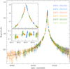 |
Fig. 1 Microlensing light curve of KMT-2021-BLG-0240. Drawn over the data points is a single-lens single-source (1L1S) model curve. The inset shows the enlargement of the peak region and the residuals from the 1L1S model. The colors of the data points are set to match those of the labels designating the telescopes used for observations marked in the legend. |
3 Anomaly in the Lensing Light Curve
The light curve of the event constructed with the photometric data from the three KMTNet telescopes are plotted in Fig. 1. From a glimpse, it would appear to be that of a normal single-lens single-source (1L1S) event with a high magnification. However, a close look at the light curve reveals that it exhibits slight deviations at the 0.1 mag level in the region around the peak. A 1L1S model and the residuals are presented in the inset of Fig. 1. The deviations appear in all three sets of the KMTS, KMTC, and KMTA data taken during the time span 9311.4 ≲ HJD′ ≲ 9313.5. We note that the gaps among the data sets appear because the peak of the event occurred during the early observing season, at which time the bulge could be observed for ~5 h. We separately show the peak region in Fig. 2 to better illustrate the deviations.
3.1 Binary-Lens (2L1S) and Source (1L2S) Interpretations
To explore the origin of the anomaly, we first test a model with two lens components (M1 and M2): 2L1S model. We check this model because the anomaly appears near the peak, for which the chance of being perturbed by a planetary companion located near the Einstein ring (Griest & Safizadeh 1998) or a binary companion with a very large or a small separation (Han et al. 2005) is high.
The 2L1S modeling is conducted to search for a solution, defined by a parameter set that best describes the observed data. Among the lensing parameters, three depict the encounter between the source and lens: t0, u0, and tE, which indicate the epoch and impact parameter of the source-lens approach, and time scale of the event, respectively. Another three parameters depict the binary lens system: s, q, and α. These parameters denote the M1–M2 separation (in projection and normalized to θE), the mass ratio, and the angle between the source motion and the binary axis, respectively. Besides these parameters, we add an extra parameter ρ (normalized source radius), denoting the angular source radius θ* in units of θE. This parameter is included to take into consideration finite-source effects that may give rise to the deformation of the anomaly during the source crossings over caustics.
The 2L1S lensing parameters were searched for using two approaches, in which the binary parameters s and q were investigated via a grid approach, and the others were derived via a downhill approach. A Markov chain Monte Carlo (MCMC) logic was used in the downhill approach. This grid search provided us a ∆χ2 map on the s–q plane, and the map enabled us to identify local minima. For each local solution, we polished the parameters, including s and q, by allowing them to vary using the MCMC approach. This approach of finding lensing solutions is useful for identifying degenerate solutions, in which different models result in similar light curves. From the modeling, it was found that a 2L1S interpretation does not yield a model that adequately explains the observed anomaly.
Recognizing that the light curve cannot be explained by a 2L1S interpretation, we then checked the possibility that the source is composed of binary stars: 1L2S model. A 1L2S modeling requires four extra lensing parameters in addition to those of a 1L1S model. These extra parameters are t0,2, u0,2, ρ2, and qF, and they represent the epoch and separation of the second source (S2) from the lens at the closest approach, the normalized radius of S2, and the flux ratio between the primary and secondary source stars, respectively. It was found that this interpretation did not yield a model describing the anomaly either. This is because the anomaly shows both positive and negative deviations from the 1L1S model, as shown in the residual presented in the bottom panel of Fig. 2, but a 1L2S model can generate only positive deviations.
We then conduct an additional modeling to check whether a 2L1S model can describe a part of the anomaly. We do this check because if the lens is composed of three masses (3L1S) or the source is a binary (2L2S), a 2L1S model can often depict a part of the anomaly, while the rest of the anomaly can be described by introducing a tertiary lens component or a companion to the source. For this check, we divide the anomaly into four regions: 9311.35 ≤ HJD′ ≤ 9312.42 (R1 region), 9312.42 ≤ HJD′ ≤ 9312.70 (R2 region), 9312.70 ≤ HJD′ ≤ 9313.00 (R3 region), and 9313.00 ≤ HJD′ ≤ 9312.48 (R4 region). The divisions of the regions are marked by dashed vertical lines in Fig. 2. The 2L1S modeling according to this scheme is done for the data excluding those in one of the four deviation regions. From the modeling conducted by excluding the data in the R3 region, we find two models that can approximately explain the deviations in the other three regions. The binary lens parameters of these models are
 (1)
(1)
The two locals are referred to as “close” and “wide” solutions because s < 1.0 and s > 1.0 for the individual solutions. The model curve and the residual of the wide 2L1S solution are shown in Fig. 2. For the two degenerate solutions, the binary separations approximately follow the relation sclose × swide ~ 1, and this suggests that the similarity between the two models originates from the close–wide degeneracy first pointed out by Griest & Safizadeh (1998) and later discussed in detail by Dominik (1999) and An (2005). For both solutions, the mass ratios between the lens components are less than 10−3, suggesting that a planetary-mass companion accompanies the primary of the lens regardless of the solutions.
Figure 3 shows the lensing configurations of the close (upper panel) and wide (lower panel) 2L1S models. For both solutions, the anomaly was produced by the source crossings over the central caustic induced by a planet lying close to the Einstein ring. Due to severe finite-source effects, the light curve during the caustic crossings induce weak deviations instead of usual sharp spike features.
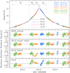 |
Fig. 2 Zoom-in view of the light curve near the peak. The vertical dashed lines denote the four regions of deviations: 9311.35 ≤ HJD′ ≤ 9312.42 (R1 region), 9312.42 ≤ HJD′ ≤ 9312.70 (R2 region), 9312.70 ≤ HJD′ ≤ 9313.00 (R3 region), and 9313.00 ≤ HJD′ ≤ 9312.48 (R4 region). The curves over the data represent the 2L2S (close), 3L1S (close–wide), 2L1S (wide), and 1L1S models, for which the residuals are shown in the lower panels. The 2L1S model is found by modeling the data excluding those in the R3 region. |
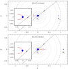 |
Fig. 3 Configurations of the close (upper panel) and wide (lower panel) 2L1S solutions found from the modeling conducted by excluding the data in the R3 deviation region, marked in Fig. 2. In each panel, the line with an arrow indicates the trajectory of the source motion, the concave closed curve is the caustic, the dashed circle denotes the Einstein ring, and the two blue dots marked by M1 and M2 indicate the positions of the lens components. The zoom-in view of the central magnification region is shown in the inset. The grey curves encompassing the caustic represent the equi-magnification contours. |
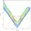 |
Fig. 4 Map of ∆χ2 on the log s3−log q3 plane. The color coding corresponds to regions with ∆χ2 ≤ 1 (red), ≤ 4 (yellow), ≤9 (green), ≤16 (cyan), and ≤25 (blue). The two regions enclosed by dashed circles constitute the two locals. |
3.2 Triple-Lens (3L1S) Interpretation
The fact that a 2L1S model partially explains the anomaly suggests that there may be a tertiary lens component, M3. This is because an anomaly induced by two companions (M2 and M3), in many cases, can be approximately described by the superposition of the 2L1S perturbations, in which the pairs of (M1, M2) and (M1, M3) behave as individual 2L lenses (Bozza 1999; Han et al. 2001). Under this approximation, then, the residual from the 2L1S model, that is, the deviation in the R3 region, may be explained by adding a tertiary lens component. For this check, we conduct a 3L1S modeling.
The 3L1S modeling was conducted in a similar fashion to the 2L1S modeling. We first found the parameters related to the tertiary lens component (s3, q3, ψ) via a grid approach by keeping the other parameters the same as those of the 2L1S solution, and then polished the locals found from the preliminary modeling by releasing all lensing parameters as free parameters. Here s3 and q3 denote the separation and mass ratio between M1 and M3, respectively, and ψ indicates the orientation angle of M3 as measured from the M1–M2 axis with a center at the position of M1. We denote the parameters describing M2 as (s2, q2) to distinguish them from those describing M3. Because a central caustic can be induced not only by a planet lying near the Einstein ring but also by a binary companion with a very large or a small separation (Lee et al. 2008), we set the ranges of s3 and q3 wide enough to consider both planetary and binary companions: [−1.5, 1.5] for log s3 and [−5.0, 0.0] for log q3.
Figure 4 shows the ∆χ2 map on the log s3–log q3 plane constructed by conducting the grid searches for these parameters with the initial 2L1S parameters adopted from those of the close 2L1S solution. The map shows two distinctive local solutions lying at

The two solutions result in similar model curves caused by the close–wide degeneracy in s3, and thus we refer them to as ‘close’ and ‘wide’ solutions. We find another two solutions obtained from the modeling with the initial parameters of the wide 2L1S solution, and thus there exist 4 solutions in total. We designate the individual solutions as close–close (s2 < 1.0 and s3 < 1.0), close–wide (s2 < 1.0 and s3 > 1.0), wide–close (s2 > 1.0 and s3 < 1.0), and wide-wide (s2 > 1.0 and s3 > 1.0) solutions. The lensing parameters of the four 3L1S models obtained under the assumption of a rectilinear relative lens-source motion (standard model) are presented in Table 1 together with the values of χ2/d.o.f. It was found that the degeneracies among the solutions are severe with ∆χ2 < 1.7. We note that it is difficult to choose a correct model based on the argument on the dynamical stability of the lens system first because both the companions are planets for which their masses are too small to affect the dynamics of the system unlike triple stellar systems (Toonen et al. 2016), and second because the measured separations are not intrinsic values but projected ones.
It is found that the 3L1S models can explain all the features of the anomaly. The model curve of the best-fit 3L1S model (close–wide model) and its residuals are presented in Fig. 2. We note that the other 3L1S solutions yield similar models to the presented one. The estimated mass ratios between the M1–M2 pair are in the range of q2 ~ [0.6−1.0] × 10−3, and those between the M1–M3 pair are in the range of q3 ~ [0.9−1.9] × 10−3. These mass ratios roughly correspond to the ratio between the Jupiter and the Sun of the Solar system. According to the 3L1S interpretation, then, the lens is a planetary system possessing two giant planets. If this interpretation is correct, the lens of the event is the sixth case of multiple planetary system found by microlensing, following OGLE-2006-BLG-109 (Gaudi et al. 2008; Bennett et al. 2010), OGLE-2012-BLG-0026 (Han et al. 2013; Beaulieu et al. 2016), OGLE-2018-BLG-1011 (Han et al. 2019), OGLE-2019-BLG-0468 (Han et al. 2022c), and KMT-2021-BLG-1077 (Han et al. 2022a).
Figure 5 shows the lensing configurations corresponding to the four 3L1S solutions. For both close-xx and wide-xx solutions, the caustics appear to be similar to those of the corresponding 2L1S solutions presented in Fig. 3, but they differ from the 2L1S caustics in the region around the planet host. See the zoom-in view of the central region shown in the right inset of each panel. In this region, there exists a tiny caustic generated by the tertiary lens component. The four empty cyan circles (labeled as t1 , t2, t3, and t4) on the source trajectory denote the source positions corresponding to the deviations in the R1 , R2, R3, and R4 regions, respectively, marked in Fig. 2. It shows that the source passed the region of positive deviations extending from a cusp of the tiny caustic induced by M3, and this explains the R3 region deviation that could not be accounted for by the two-mass lens model.
We checked higher-order effects causing nonrectilinear relative motion between the source and lens. Two major effects cause deviations from the rectilinear motion: microlens-parallax and lens-orbital effects. The former effect arises due to the Earth’s (observer’s) orbital motion around the Sun (Gould 1992), and the latter effect arises due to the orbital motion of the lens (Dominik 1998). We found that specifying the lens orbital motion was difficult because the anomaly lasted for a very short period of time, and thus only the parallax effect was considered in the modeling. The extra parameters required to define the microlens-parallax effect are the two components (πE,N for the north direction and πE,E for the east direction) of the microlens-lens parallax vector πE = (πrel/θE)(μ/μ), where  represents the relative lens-source parallax, DL and DS represent the distances to the lens and source, respectively, and μ is the relative lens-source proper motion. We investigated whether microlens parallax could be constrained, but it was found that the small parallax signal was not consistent between observatories and therefore was most likely due to low-level systematics, which often dominate the parallax signals for events with faint source stars.
Lensing parameters of 3L1S solutions.
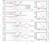 |
Fig. 5 Lensing configurations of the four 3L1S solutions: close–close, close–wide, wide–close, and wide–wide solutions. The right inset in each panel displays the magnified view around the planet host. The four empty cyan circles on the source trajectory (labeled as t1, t2, t3, and t4) denote the source positions corresponding to the deviations in the R1, R2, R3, and R4 regions. The circle size is scaled to θE corresponding to the total mass of the lens. The grey curves represent the equi-magnification contours. |
Lensing parameters of 2L2S model.
3.3 Binary-Lens Binary-Source (2L2S) Interpretation
It is known that a 3L1S model can occasionally be degenerate with a 2L2S model, in which both the lens and source are binaries, as illustrated in the cases of the lensing events KMT-2019-BLG-1953 (Han et al. 2020a) and OGLE-2018-BLG-0532 (Ryu et al. 2020). For the investigation of this degeneracy, we additionally conducted a 2L2S modeling of the event. In this modeling, we started with the lensing parameters of the 2L1S model explaining the anomaly features except the R3 region, and checked a possible trajectory of S2 explaining the anomaly in the R3 region.
From the 2L2S modeling, we found two solutions that well explain all of the anomaly features. The individual solutions were found based on the close and wide 2L1S solutions, and thus we designate them as “close” and “wide” solutions. The close model yields a slightly better fit to the data, but the difference is very small with ∆χ2 = 0.5. The model curve and residual of the close 2L2S solution are shown in Fig. 2, and the lensing parameters of both solutions are listed in Table 2. In the table, we use the notations (t0,1, u0,1, ρ1) to denote the lensing parameters related to the primary source S1. The 2L2S model curve differs from that of the 3L1S model in the time domain 9312.9 ≲ HJD′ ≲ 9313.1, but this region corresponds to the gap between the KMTC and KMTA data sets.
Figure 6 shows the lens system configurations of the close (upper panel) and wide (lower panel) 2L2S models. They are similar to the configurations of the corresponding 2L1S models, presented in Fig. 3, except that there are two source trajectories, which are marked as S1 for the primary source and S2 for the secondary source. It is estimated that the ratios of the I-band flux from the second source to the flux from the primary are qF,I = 0.18 and 0.14 according to the close and wide solutions, respectively. In both cases, the second source, which lay very close to the primary source, moved in parallel with the primary source, and crossed the caustics almost at the same times of the primary source caustic crossings, and thus the caustic crossings of S2 did not exhibit extra caustic-crossing features. However, the second source additionally passed over the tiny cusp lying very close to the primary lens, and this gives rise to an extra anomaly feature that explains the deviation in the R3 region.
It is found that the 2L2S models yield better fits than the 3L1S models by ∆χ2 = [10.8 − 12.5]. If the 2L2S interpretation is correct, KMT-2021-BLG-0240 is the sixth lensing event for which both the lens and source are binaries, following MOA-2010-BLG-117 (Bennett et al. 2018), OGLE-2016-BLG-1003 (Jung et al. 2017), KMT-2018-BLG-1743 (Han et al. 2021a), KMT-2019-BLG-0797 (Han et al. 2021b), and KMT-2021-BLG-1898 (Han et al. 2022b). Except for OGLE-2016-BLG-1003, the lenses of the other five events, including the event analyzed in this work, are planetary systems, indicating that planetary signals detectable through the high-magnification channel are prone to be affected by close companions to source stars.
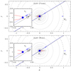 |
Fig. 6 Lensing configurations of the two 2L2S models. Notations are same as those in Fig. 3, except that there are two source trajectories, which are marked by S1 for the primary source and S2 for the secondary source. The two source trajectories in the main panel are difficult to distinguish due to the closeness of the trajectories, and thus we present the enlargement of the central region in the inset. The trajectories of the primary (S1) and secondary (S2) source stars are marked in black and blue lines, respectively. The empty circles on the individual source trajectories indicate the source sizes estimated from the 2L2S modeling. |
3.4 3L1S Versus 2L2S Interpretations
According to the 2L2S model, the closeness of the source stars should induce large effects on the anomaly caused by the orbital motion of the binary source unless they are seen in extreme projection. Under the assumption that the binary source orbit is seen face on, the separation between S1 and S2 is  , where ∆τ = (t0,1 − t0,2)/tE and ∆u0 = u0,1 − u0,2. As will be discussed in Sect. 4, the angular Einstein radius and the relative lens-source proper motion estimated from the 2L2L solution are θE ~ 0.44 mas and μrel ~ 3.9 mas yr−1, respectively. Then, the projected physical separation between the two source stars is ∆a⊥ = DSθE∆u ~ 0.016 AU. Assuming that
  and
and  , this creates an orbital period P, an internal velocity υint, and an internal proper motion μint of
 ![$P = {\left\{ {{{{{\left( {{{{a_ \bot }} \mathord{\left/ {\vphantom {{{a_ \bot }} {{\rm{AU}}}}} \right. \kern-\nulldelimiterspace} {{\rm{AU}}}}} \right)}^3}} \mathord{\left/ {\vphantom {{{{\left( {{{{a_ \bot }} \mathord{\left/ {\vphantom {{{a_ \bot }} {{\rm{AU}}}}} \right. \kern-\nulldelimiterspace} {{\rm{AU}}}}} \right)}^3}} {\left[ {{{\left( {{M_{{S_1}}} + {M_{{S_2}}}} \right)} \mathord{\left/ {\vphantom {{\left( {{M_{{S_1}}} + {M_{{S_2}}}} \right)} {{M_ \odot }}}} \right. \kern-\nulldelimiterspace} {{M_ \odot }}}} \right]}}} \right. \kern-\nulldelimiterspace} {\left[ {{{\left( {{M_{{S_1}}} + {M_{{S_2}}}} \right)} \mathord{\left/ {\vphantom {{\left( {{M_{{S_1}}} + {M_{{S_2}}}} \right)} {{M_ \odot }}}} \right. \kern-\nulldelimiterspace} {{M_ \odot }}}} \right]}}} \right\}^{{1 \mathord{\left/ {\vphantom {1 2}} \right. \kern-\nulldelimiterspace} 2}}} \sim 1.6 \times {10^{ - 3}}{\rm{yr = 0}}{\rm{.58}}$](/articles/aa/full_html/2022/08/aa43161-22/aa43161-22-eq8.png) days, υint = (a/P)υ⊕ ~ 300 km s−1, and μint = υint/DS ~ 7.9 mas yr−1, respectively. Here (MS,1, MS,2) denote the masses of the source stars, and υ⊕ = 30 km s−1 is the orbital speed of Earth around the Sun. Then, the internal motion induced by the source orbital motion is twice faster than the relative lens-source proper motion estimated from the normalized source radius ρ, that is, μrel ~ 3.9 mas yr−1. This implies that the normalized source radius estimated under static and orbiting source can be different by a factor 2. Moreover, the positional change of the primary source during P/2 = 0.29 days in units of θE is
days, υint = (a/P)υ⊕ ~ 300 km s−1, and μint = υint/DS ~ 7.9 mas yr−1, respectively. Here (MS,1, MS,2) denote the masses of the source stars, and υ⊕ = 30 km s−1 is the orbital speed of Earth around the Sun. Then, the internal motion induced by the source orbital motion is twice faster than the relative lens-source proper motion estimated from the normalized source radius ρ, that is, μrel ~ 3.9 mas yr−1. This implies that the normalized source radius estimated under static and orbiting source can be different by a factor 2. Moreover, the positional change of the primary source during P/2 = 0.29 days in units of θE is  , which is similar to u0. Considering that the effective time scale of the event is teff = u0tE ~ 0.18 days, the light curve would show extremely violent (factor 2) changes by the orbital motion of the source during ~[−teff, +teff], but no such changes were observed.
The 2L2S solution is further disfavored by the absence of ellipsoidal variations. If the binary source stars are closely separated as measured by the 2L2S solutions, the source would be distorted by tides and the light curve would therefore show ellipsoidal variations, but no such variations are seen in the light curve. These problems can be avoided by the assumption that the binary is seen in projection or the orbital plane is perpendicular to the direction of lens-source. This argument requires that the proper motion induced by the binary source orbit to be at least 6 times smaller than the relative lens-source proper motion. This can be achieved with a projection factor of 200 (probability: ~ 1/80 000), or for example, by projection factor of 5 but orbital alignment within about 10° of perpendicular (probability: ~ 1/450).
In order to have confidence in the very low-probability binary-source configurations, one would need high statistical confidence. However, the signal is rather weak for such an analysis. Furthermore, there is an alternative 3L1S solution that is disfavored by only ∆χ2 ~ 10, which is small given the quality of the data. Therefore, we conclude that the 3L1S and 2L2S solutions cannot be distinguished with the available data, and either could be correct. However, we note that the detection of one planet, M2 for the 3L1S model, is solid regardless of the solutions. In the following analysis, we estimate the physical lens parameters for both interpretations of the event.
Because of the possible importance of the source orbital motion together with no clear features of sharp caustic crossings, the observed anomaly could be, in principle, entirely due to “xallarap” effects, that is, the orbital effect induced by a source companion whose own luminosity contributes negligibly to the light curve of a single-lens event. Motivated by this consideration, we check whether the anomaly could be due to xallarap effects alone. The modeling considering the xallarap effect requires 5 additional parameters in addition to the 1L1S parameters: ξE,N, ξE,E, P, ϕ, and i (Dong et al. 2009). The parameters (ξE,N,ξE,E) denote the north and east components of the xallarap vector ξE, P is the orbital period, and (ϕ, i) denote the phase and inclination angles of the orbit, respectively. The magnitude of ξE is related to the semi-major axis, a, of the source orbit by ξE = aS/(DSθE), where aS = aMS,2/(MS,1 + MS,2). Considering the short duration of the anomaly, we test xallarap models with orbital periods within the range of 0.1 ≤ P/days ≤ 10. We find that the fits of the xallarap models are worse than the 3L1S and the static 2L2S models by ∆χ2 ~ 42 and ~53, respectively, and thus we conclude that the anomaly cannot be attributed to the xallarap effect.
4 Source Star and Angular Einstein Radius
In this section, we estimate the extra observable of θE according to the 3L1S and 2L2S solutions. For both solutions, θE measurement is possible because the source star crossed the caustic and the light curve around these epochs was impacted by the effect of a finite source size. The measured normalized source radius allows one to estimate the Einstein radius (Gould 1994; Witt & Mao 1994; Nemiroff & Wickramasinghe 1994) as
 (3)
(3)
For the measurement of θE, one needs to measure θ*, which is inferred from the color and brightness of the source. For the estimation of the source color, it is required to measure the source magnitudes in two passbands, V and I in our case, from the regression of the photometric data to the model of the lensing light curve. For KMT-2021-BLG-0240, we could measure the I-band magnitude precisely, but it was difficult to measure a reliable V-band magnitude because of the poor quality of the V-band data caused by the heavy extinction toward the field. Due to this difficulty, we interpolate the source color from the main-sequence branch of stars in the color-magnitude diagram (CMD) built from the observations using the Hubble Space Telescope (HST; Holtzman et al. 1998) based on the measured I-band magnitude.
Figure 7 shows the location of the source star in the CMD constructed from the combination of HST and ground-based observations. The ground-based CMD was built using the pyDIA photometry of the KMTC data, and the HST and KMTC CMDs were aligned utilizing the centroids of the red giant clump (RGC) on the individual CMDs. In the CMD, the small filled dot marked in magenta indicates the source position according to the 3L1S solution, and the blue and green dots represent the positions of the primary and secondary source stars estimated from the 2L2S solution, respectively. In the case of the 2L2S solution, the I-band magnitudes of the two source stars were estimated from the combined flux FS, I, which was measured from the modeling, by

where qF,I is the flux ratio between the two source stars, and  and
and  indicate flux values of S1 and S2, respectively. The measured values of the instrumental (uncalibrated) color and magnitude are
 (5)
(5)

for the 2L2S solution, and
 (7)
(7)
for the RGC centroid commonly for the both solutions. Also marked in the CMD is the location of a blend (black filled dot). It shows that the observed flux is affected by blended light that is almost as bright as the source.
Calibration of the source color and magnitude was done by applying the method of Yoo et al. (2004), which utilizes the RGC centroid with its known dereddened color and magnitude, (V − I, I)RGC,0. Following this method, the dereddened values of the source were estimated using the known values of the RGC centroid, (V − I)RGC,0 = (1.06, 14.45) (Bensby et al. 2013; Nataf et al. 2013), and the offsets between the source and RGC centroid, ∆(V − I, I) = (V − I, I)S − (V − I, I)rgc, by (V − I, I)S,0 = (V − I, I)RGC,0 + ∆(V − I, I). The dereddened values of the color and magnitude for the source estimated from this calibration process are
 (8)
(8)
for the 3L1S solution, and
 (9)
(9)
for the 2L2S solution. According to the 3L1S solution, the source is a subgiant or a turnoff star of an early G spectral type. According to the 2L2S solution, the secondary source is a late G dwarf and the spectral type of the primary source is similar to that of the 3L1S solution but slightly bluer and fainter.
With the measured normalized source radius, we estimated the angular Einstein radius using the relation in Eq. (3). For the 2L2S solution, the Einstein radius can be estimated either by  or
or  , where
  and
and  represent the angular source radii of S1 and S2, respectively. We choose to estimate θE using the former relation because both the stellar type and normalized source radius of the primary source are better constrained than those of the secondary source. For the estimation of the source radius, we first converted V − I color into V − K color using the Bessell & Brett (1988) relation, and then assessed θ* with the application of the Kervella et al. (2004) relation between V − K and θ*. The source radii assessed from this procedure are
 (10)
(10)
for the 3L1S and 2L2S solutions, respectively. From the relation in Eq. (3), we estimate the Einstein radius as
 (11)
(11)
The relative proper motion between the lens and source is estimated by μrel = θE/tE, and the values resulting from the θE values in Eq. (11) are
 (12)
(12)
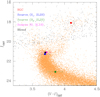 |
Fig. 7 Color-magnitude diagram (CMD) constructed from the combination of the HST and ground-based (KMTNet) observations. The small filled dot marked in magenta indicates the source position according to the 3L1S solution, and the blue and green dots represent the positions of the primary and secondary source stars estimated from the 2L2S solution, respectively. The red dot denotes the centroid of red giant clump (RGC). |
5 Physical Parameters of Planetary System
The physical parameters of a lens system can be constrained by the lensing observables including tE, θE, and πE. Measurements of all these observables enable one to uniquely determine the physical parameters as
 (13)
(13)
where к = 4G/(c2AU), and πS = AU/DS is the parallax of the source. For KMT-2021-BLG-0240, the value of πE cannot be securely measured, although the tE and θE observables are precisely measured. Therefore, we estimate M and DL from a Bayesian analysis utilizing a Galactic model based on the constraints given by the measured observables.
In the Bayesian analysis, we generate many artificial lensing lensing events by performing a Monte Carlo simulation, in which the locations and motions of sources and lenses and the masses of lenses are assigned based on a Galactic model. In the simulation, we used the Jung et al. (2021) Galactic model, which was constructed using the models of Robin et al. (2003) and Han & Gould (2003) for the physical distributions of disk and bulge objects, respectively, the models of Jung et al. (2021) and Han & Gould (1995) for the dynamical distributions for disk and bulge objects, respectively, and the model of Jung et al. (2018) for the common mass function of disk and bulge lenses. The Bayesian posteriors are constructed for the simulated events having observables lying in the ranges of the measured values. As mentioned, the value of the microlens parallax cannot be reliably determined for either the 3L1S or the 2L2S solutions, and thus we use the constraints of tE and θE in the Bayesian analysis.
Figure 8 shows the Bayesian posteriors for the mass of the planet host (upper panel) and distance to the planetary system (lower panel). The distributions for the 3L1S and 2L2S solutions are marked in blue and red, respectively. Because of the larger θE value, the mass estimated from the 2L2S solution is slightly larger than the mass assessed from the 3L1S solution. For the same reason, the distance to the lens for the 2L2S solution is slightly smaller than the distance for the 3L1S solution.
In Table 3, we list the physical parameters of the planetary system estimated based on the 3L1S and 2L2S solutions. Common parameters for both solutions include the masses of the host, M1, and the confirmed planet, M2, distance, DL, and projected separation between M1 and M2, a⊥(M1–M2). For the 3L1S solution, additional parameters of the mass of the not-confirmed second planet, M3, and the projected separation between M1 and M3, a⊥(M1–M3), are listed. According to the 3L1S solution, the lens is a planetary system with two sub-Jovian-mass planets, in which the planets have masses of 0.32–0.47 MJ and 0.44–0.93 MJ orbiting an M dwarf host. According to the 2L2S solution, the lens is a planetary system in which a single planet with a mass of ~0.21 MJ orbits a late K-dwarf host. The distance to the planetary system varies depending on the solution: ~7.0 kpc for the 3L1S solution and ~6.6 kpc for the 3L1S solution.
Although the two solutions cannot be distinguished based on present data, the degeneracy can in principle be broken by future radial velocity (RV) observations. Such observations would find the two q ~ 10−3 planets if the 3L1S solution is correct, but only one such planet if the 2L2S solution is correct. The first step would be to resolve the host, which will be possible at first adaptive-optics (AO) light on next-generation (that is, 30 m class) telescopes. For example, by 2030, the source and lens will be separated by the order of 30 mas, according to Eq. (12). Scaling from the experience with current 8 m to 10 m telescopes, it should be possible to determine the mass, distance and infrared brightness of the host. Based on these results, it can be determined whether RV observations are feasible with these next-generation telescopes or will have to wait for further generations of telescopes, that is, of 100 m diameter. Regardless, the wait time is likely to be less than the 57 yr between the year that Einstein (1936) argued that there would be no great chance of observing this phenomenon and that of the first detection of a microlensing event (Alcock et al. 1993; Udalski et al. 1993).
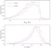 |
Fig. 8 Bayesian posteriors of the host mass and the distance to the planetary system. The curves drawn in blue and red represent the distributions estimated from the 3L1S and 2L2S solutions, respectively. |
Physical lens parameters.
6 Summary and Conclusion
We investigated the lensing event KMT-2021-BLG-0240, for which the light curve was densely and continuously covered from the high-cadence observations using the globally distributed three telescopes of the KMTNet survey conducted in the 2021 season. The light curve from a glimpse appeared to be that of a regular lensing event produced by a single mass magnifying a single source star, but a close look revealed an anomaly with complex features at the 0.1 mag level lasted for ~2 days in the region around the peak.
It was found that the anomaly could not be explained with either a 2L1S or a 1L2S model, which are the most common causes of microlensing anomalies. However, we found that a 2L1S model could describe a part of the anomaly, suggesting the possibility that the anomaly might be deformed by a tertiary lens component or a close companion to the source. From the additional modeling, we found that all the features of the anomaly could be explained with either a 3L1S model or a 2L2S model. In the sense of the goodness of the fit, the 2L2S interpretation was slightly preferred over the 3L1S interpretation. However, the 2L2S interpretation was less favored due to the absence of signatures induced by the source orbital motion and ellipsoidal variations. We, therefore, conclude that the two interpretations could not be distinguished with the available data, and either could be correct.
According to the 3L1S solution, the lens is a planetary system with two sub-Jovian-mass planets, in which the planets have masses of 0.32–0.47 MJ and 0.44–0.93 MJ and they orbit an M dwarfhost. According to the 2L2S solution, on the otherhand, the lens is a single planet system with a ~0.21 MJ planet orbiting a late K-dwarf host, and the source is a binary composed of a primary of a subgiant or a turnoff star and a secondary of a late G dwarf. The distance to the planetary system varies depending on the solution: ~7.0 kpc for the 3L1S solution and ~6.6 kpc for the 2L2S solution.
Acknowledgements
Work by C.H. was supported by the grants of National Research Foundation of Korea (2020R1A4A2002885 and 2019R1A2C2085965). J.C.Y. acknowledges support from N.S.F Grant No. AST-2108414. This research has made use of the KMTNet system operated by the Korea Astronomy and Space Science Institute (KASI) and the data were obtained at three host sites of CTIO in Chile, SAAO in South Africa, and SSO in Australia.
References
- Alard, C., & Lupton, R.H. 1998, ApJ, 503, 325 [NASA ADS] [CrossRef] [Google Scholar]
- Albrow, M. 2017, https://doi.org/18.5281/zenodo.268849 [Google Scholar]
- Albrow, M., Horne, K., Bramich, D.M., et al. 2009, MNRAS, 397, 2099 [NASA ADS] [CrossRef] [Google Scholar]
- Alcock, C. Akerlof, C.W., Allsman, R.A., et al. 1993, Nature, 365, 621 [NASA ADS] [CrossRef] [Google Scholar]
- An, J.H. 2005, MNRAS, 356, 1409 [NASA ADS] [CrossRef] [Google Scholar]
- Beaulieu, J.-P., Bennett, D.P., Batista, V., et al. 2016, ApJ, 824, 83 [CrossRef] [Google Scholar]
- Bennett, D.P., Rhie, S.H., Nikolaev, S., et al. 2010, ApJ, 713, 837 [NASA ADS] [CrossRef] [Google Scholar]
- Bennett, D.P., Rhie, S.H., Udalski, A., et al. 2016, AJ, 152, 125 [NASA ADS] [CrossRef] [Google Scholar]
- Bennett, D.P., Udalski, A., Han, C., et al. 2018, AJ, 155, 141 [NASA ADS] [CrossRef] [Google Scholar]
- Bensby, T., Yee, J.C., Feltzing, S., et al. 2013, A&A, 549, A147 [NASA ADS] [CrossRef] [EDP Sciences] [Google Scholar]
- Bessell, M.S., & Brett, J.M. 1988, PASP, 100, 1134 [NASA ADS] [CrossRef] [Google Scholar]
- Bond, I.A., Abe, F., Dodd, R.J., et al. 2001, MNRAS, 327, 868 [NASA ADS] [CrossRef] [Google Scholar]
- Bozza, V. 1999, A&A, 348, 311 [NASA ADS] [Google Scholar]
- Danek, K., & Heyrovsky, D. 2015, ApJ, 806, 99 [CrossRef] [Google Scholar]
- Danek, K., & Heyrovsky, D. 2019, ApJ, 880, 72 [CrossRef] [Google Scholar]
- Dominik, M. 1998, A&A, 329, 361 [NASA ADS] [Google Scholar]
- Dominik, M. 1999, A&A, 349, 108 [NASA ADS] [Google Scholar]
- Dong, S., Gould, A., Udalski, A., et al. 2009, ApJ, 695, 970 [NASA ADS] [CrossRef] [Google Scholar]
- Einstein, A. 1936, Science, 84, 506 [NASA ADS] [CrossRef] [Google Scholar]
- Gaudi, B.S., & Gould, A. 1997, ApJ, 486, 85 [NASA ADS] [CrossRef] [Google Scholar]
- Gaudi, B.S., Naber, R.M., & Sackett, P.D. 1998, ApJ, 502, L33 [CrossRef] [Google Scholar]
- Gaudi, B.S., Bennett, D.P., Udalski, A., et al. 2008, Science, 319, 927 [NASA ADS] [CrossRef] [Google Scholar]
- Gould, A. 1992, ApJ, 392, 442 [Google Scholar]
- Gould, A. 1994, ApJ, 421, L75 [NASA ADS] [CrossRef] [Google Scholar]
- Gould, A., & Loeb, A. 1992, ApJ, 396, 104 [Google Scholar]
- Gould, A., Dong, S., Gaudi, B.S., et al. 2010, ApJ, 720, 1073 [NASA ADS] [CrossRef] [Google Scholar]
- Griest, K., & Safizadeh, N. 1998, ApJ, 500, 37 [Google Scholar]
- Han, C. 2005, ApJ, 629, 1102 [NASA ADS] [CrossRef] [Google Scholar]
- Han, C. 2006, ApJ, 638, 1080 [Google Scholar]
- Han, C., & Gould, A. 1995, ApJ, 447, 53 [Google Scholar]
- Han, C., & Gould, A. 2003, ApJ, 592, 172 [Google Scholar]
- Han, C., Chang, H.-Y., An, J.H., & Chang, K. 2001, MNRAS, 328, 986 [NASA ADS] [CrossRef] [Google Scholar]
- Han, C., Gaudi, B.S., An, J.H., & Gould, A. 2005, ApJ, 618, 962 [NASA ADS] [CrossRef] [Google Scholar]
- Han, C., Udalski, A., Choi, J.-Y., et al. 2013, ApJ, 762, L28 [Google Scholar]
- Han, C., Udalski, A., Gould, A., et al. 2017, AJ, 154, 223 [Google Scholar]
- Han, C., Bennett, D.P., Udalski, A., et al. 2019, AJ, 158, 114 [NASA ADS] [CrossRef] [Google Scholar]
- Han, C., Kim, D., Jung, Y.K., et al. 2020a, AJ, 160, 17 [NASA ADS] [CrossRef] [Google Scholar]
- Han, C., Lee, C.-U., Udalski, A., et al. 2020b, AJ, 159, 48 [Google Scholar]
- Han, C., Albrow, M.D., Chung, S.-J., et al. 2021a, A&A, 652, A145 [NASA ADS] [CrossRef] [EDP Sciences] [Google Scholar]
- Han, C., Lee, C.-U., Ryu, Y.-H. 2021b, A&A, 649, A91 [NASA ADS] [CrossRef] [EDP Sciences] [Google Scholar]
- Han, C., Gould, A., Bond, I. et al. 2022a, A&A, 662, A70 [NASA ADS] [CrossRef] [EDP Sciences] [Google Scholar]
- Han, C., Gould, A., Kim, D., et al. 2022b, A&A, 663, A145 [NASA ADS] [CrossRef] [EDP Sciences] [Google Scholar]
- Han, C., Udalski, A., Lee, C.-U., et al. 2022c, A&A, 658, A93 [NASA ADS] [CrossRef] [EDP Sciences] [Google Scholar]
- Holtzman, J.A., Watson, A.M., Baum, W.A., et al. 1998, AJ, 115, 1946 [NASA ADS] [CrossRef] [Google Scholar]
- Jung, Y.K., Udalski, A., Bond, I.A., et al. 2017, ApJ, 841, 75 [NASA ADS] [CrossRef] [Google Scholar]
- Jung, Y.K., Udalski, A., Gould, A., et al. 2018, AJ, 155, 219 [NASA ADS] [CrossRef] [Google Scholar]
- Jung, Y.K., Han, C., Udalski, A., et al. 2021, AJ, 161, 293 [NASA ADS] [CrossRef] [Google Scholar]
- Kervella, P., Thévenin, F., Di Folco, E., & Ségransan, D. 2004, A&A, 426, 29 [Google Scholar]
- Kim, S.-L., Lee, C.-U., Park, B.-G., et al. 2016, J. Kor. Astron. Soc., 49, 37 [NASA ADS] [CrossRef] [Google Scholar]
- Lee, D.-W., Lee, C.-U., Park, B.-G., 2008, ApJ, 672, 623 [NASA ADS] [CrossRef] [Google Scholar]
- Mao, S., & Paczynski, B. 1991, ApJ, 374, L37 [NASA ADS] [CrossRef] [Google Scholar]
- Nataf, D.M., Gould, A., Fouqué, P., et al. 2013, ApJ, 769, 88 [NASA ADS] [CrossRef] [Google Scholar]
- Nemiroff, R.J., & Wickramasinghe, W.A.D.T. 1994, ApJ, 424, L21 [NASA ADS] [CrossRef] [Google Scholar]
- Robin, A.C., Reylé, C., Derriére, S., & Picaud, S. 2003, A&A, 409, 523 [NASA ADS] [CrossRef] [EDP Sciences] [Google Scholar]
- Ryu, Y.-H., Udalski, A., Yee, J.C., et al. 2020, AJ, 160, 183 [NASA ADS] [CrossRef] [Google Scholar]
- Toonen, S., Hamers, A., & Portegies Zwart, S. 2016, Comput. Astrophys. Cosmol., 3, 36 [NASA ADS] [CrossRef] [Google Scholar]
- Udalski, A., Szymanski, M., Kaluzny, J., et al. 1993, Acta Astron., 43, 289 [NASA ADS] [Google Scholar]
- Udalski, A., Jaroszynski, M., Paczynski, B., et al. 2005, ApJ, 628, L109 [NASA ADS] [CrossRef] [Google Scholar]
- Witt, H.J., & Mao, S. 1994, ApJ, 430, 505 [NASA ADS] [CrossRef] [Google Scholar]
- Yee, J.C., Shvartzvald, Y., Gal-Yam, A., et al. 2012, ApJ, 755, 102 [NASA ADS] [CrossRef] [Google Scholar]
- Yoo, J., DePoy, D.L., Gal-Yam, A., et al. 2004, ApJ, 603, 139 [NASA ADS] [CrossRef] [Google Scholar]
- Zang, W., Han, C., Kondo, I., et al. 2021, Res. Astro. Astrophys., 21, 239 [CrossRef] [Google Scholar]
All Tables
All Figures
|
Fig. 1 Microlensing light curve of KMT-2021-BLG-0240. Drawn over the data points is a single-lens single-source (1L1S) model curve. The inset shows the enlargement of the peak region and the residuals from the 1L1S model. The colors of the data points are set to match those of the labels designating the telescopes used for observations marked in the legend. |
| In the text | |
|
Fig. 2 Zoom-in view of the light curve near the peak. The vertical dashed lines denote the four regions of deviations: 9311.35 ≤ HJD′ ≤ 9312.42 (R1 region), 9312.42 ≤ HJD′ ≤ 9312.70 (R2 region), 9312.70 ≤ HJD′ ≤ 9313.00 (R3 region), and 9313.00 ≤ HJD′ ≤ 9312.48 (R4 region). The curves over the data represent the 2L2S (close), 3L1S (close–wide), 2L1S (wide), and 1L1S models, for which the residuals are shown in the lower panels. The 2L1S model is found by modeling the data excluding those in the R3 region. |
| In the text | |
|
Fig. 3 Configurations of the close (upper panel) and wide (lower panel) 2L1S solutions found from the modeling conducted by excluding the data in the R3 deviation region, marked in Fig. 2. In each panel, the line with an arrow indicates the trajectory of the source motion, the concave closed curve is the caustic, the dashed circle denotes the Einstein ring, and the two blue dots marked by M1 and M2 indicate the positions of the lens components. The zoom-in view of the central magnification region is shown in the inset. The grey curves encompassing the caustic represent the equi-magnification contours. |
| In the text | |
|
Fig. 4 Map of ∆χ2 on the log s3−log q3 plane. The color coding corresponds to regions with ∆χ2 ≤ 1 (red), ≤ 4 (yellow), ≤9 (green), ≤16 (cyan), and ≤25 (blue). The two regions enclosed by dashed circles constitute the two locals. |
| In the text | |
|
Fig. 5 Lensing configurations of the four 3L1S solutions: close–close, close–wide, wide–close, and wide–wide solutions. The right inset in each panel displays the magnified view around the planet host. The four empty cyan circles on the source trajectory (labeled as t1, t2, t3, and t4) denote the source positions corresponding to the deviations in the R1, R2, R3, and R4 regions. The circle size is scaled to θE corresponding to the total mass of the lens. The grey curves represent the equi-magnification contours. |
| In the text | |
|
Fig. 6 Lensing configurations of the two 2L2S models. Notations are same as those in Fig. 3, except that there are two source trajectories, which are marked by S1 for the primary source and S2 for the secondary source. The two source trajectories in the main panel are difficult to distinguish due to the closeness of the trajectories, and thus we present the enlargement of the central region in the inset. The trajectories of the primary (S1) and secondary (S2) source stars are marked in black and blue lines, respectively. The empty circles on the individual source trajectories indicate the source sizes estimated from the 2L2S modeling. |
| In the text | |
|
Fig. 7 Color-magnitude diagram (CMD) constructed from the combination of the HST and ground-based (KMTNet) observations. The small filled dot marked in magenta indicates the source position according to the 3L1S solution, and the blue and green dots represent the positions of the primary and secondary source stars estimated from the 2L2S solution, respectively. The red dot denotes the centroid of red giant clump (RGC). |
| In the text | |
|
Fig. 8 Bayesian posteriors of the host mass and the distance to the planetary system. The curves drawn in blue and red represent the distributions estimated from the 3L1S and 2L2S solutions, respectively. |
| In the text | |
Current usage metrics show cumulative count of Article Views (full-text article views including HTML views, PDF and ePub downloads, according to the available data) and Abstracts Views on Vision4Press platform.
Data correspond to usage on the plateform after 2015. The current usage metrics is available 48-96 hours after online publication and is updated daily on week days.
Initial download of the metrics may take a while.