| Issue |
A&A
Volume 664, August 2022
|
|
|---|---|---|
| Article Number | A13 | |
| Number of page(s) | 22 | |
| Section | Catalogs and data | |
| DOI | https://doi.org/10.1051/0004-6361/202243744 | |
| Published online | 08 August 2022 | |
Systematic KMTNet planetary anomaly search
V. Complete sample of 2018 prime-field
1
Max-Planck-Institute for Astronomy,
Königstuhl 17,
69117
Heidelberg, Germany
2
Department of Astronomy, Ohio State University,
140 W. 18th Ave.,
Columbus,
OH 43210, USA
3
Department of Physics, Chungbuk National University,
Cheongju
28644,
Republic of Korea
e-mail: This email address is being protected from spambots. You need JavaScript enabled to view it.
4
Department of Astronomy, Tsinghua University,
Beijing
100084,
PR China
5
Korea Astronomy and Space Science Institute,
Daejon
34055,
Republic of Korea
6
Astronomical Observatory, University of Warsaw,
Al. Ujazdowskie 4,
00-478
Warszawa, Poland
7
Institute of Natural and Mathematical Science, Massey University,
Auckland
0745,
New Zealand
8
University of Canterbury, Department of Physics and Astronomy,
Private Bag 4800,
Christchurch
8020,
New Zealand
9
Department of Particle Physics and Astrophysics, Weizmann Institute of Science,
Rehovot
76100,
Israel
10
Center for Astrophysics | Harvard & Smithsonian,
60 Garden St.,
Cambridge,
MA 02138,
USA
11
School of Space Research, Kyung Hee University,
Yongin,
Kyeonggi
17104,
Republic of Korea
12
Korea University of Science and Technology, Korea, (UST),
217 Gajeong-ro, Yuseong-gu,
Daejeon,
34113,
Republic of Korea
13
Department of Physics, University of Warwick,
Gibbet Hill Road,
Coventry
CV4 7AL, UK
14
Institute for Space-Earth Environmental Research, Nagoya University,
Nagoya
464-8601,
Japan
15
Code 667, NASA Goddard Space Flight Center,
Greenbelt,
MD 20771,
USA
16
Department of Astronomy, University of Maryland,
College Park,
MD 20742,
USA
17
Department of Earth and Planetary Science, Graduate School of Science, The University of Tokyo,
7-3-1 Hongo, Bunkyo-ku,
Tokyo
113-0033,
Japan
18
Instituto de Astrofísica de Canarias,
Via Láctea s/n, 38205 La Laguna,
Tenerife, Spain
19
Department of Earth and Space Science, Graduate School of Science, Osaka University,
Toyonaka,
Osaka
560-0043,
Japan
20
Department of Physics, The Catholic University of America,
Washington,
DC 20064, USA
21
Department of Astronomy, Graduate School of Science, The University of Tokyo,
7-3-1 Hongo, Bunkyo-ku,
Tokyo
113-0033,
Japan
22
Sorbonne Université, CNRS, UMR 7095, Institut d’Astrophysique de Paris,
98 bis bd Arago,
75014
Paris, France
23
Department of Physics, University of Auckland,
Private Bag
92019,
Auckland, New Zealand
24
University of Canterbury Mt. John Observatory,
PO Box 56,
Lake Tekapo
8770, New Zealand
25
IPAC,
Mail Code 100-22, Caltech, 1200 E. California Blvd.,
Pasadena,
CA 91125,
USA
26
Jet Propulsion Laboratory, California Institute of Technology,
4800 Oak Grove Drive,
Pasadena,
CA 91109,
USA
27
Department of Physics and Astronomy, Louisiana State University,
Baton Rouge,
LA 70803,
USA
28
Department of Physics & Astronomy, Vanderbilt University,
Nashville,
TN 37235,
USA
Received:
9
April
2022
Accepted:
17
May
2022
Abstract
We complete the analysis of all 2018 prime-field microlensing planets identified by the Korea Microlensing Telescope Network (KMTNet) Anomaly Finder. Among the ten previously unpublished events with clear planetary solutions, eight are either unambiguously planetary or are very likely to be planetary in nature: OGLE-2018-BLG-1126, KMT-2018-BLG-2004, OGLE-2018-BLG-1647, OGLE-2018-BLG-1367, OGLE-2018-BLG-1544, OGLE-2018-BLG-0932, OGLE-2018-BLG-1212, and KMT-2018-BLG-2718. Combined with the four previously published new Anomaly Finder events and 12 previously published (or in preparation) planets that were discovered by eye, this makes a total of 24 2018 prime-field planets discovered or recovered by Anomaly Finder. Together with a paper in preparation on 2018 subprime planets, this work lays the basis for the first statistical analysis of the planet mass-ratio function based on planets identified in KMTNet data. By systematically applying the heuristic analysis to each event, we identified the small modification in their formalism that is needed to unify the so-called close-wide and inner-outer degeneracies.
Key words: gravitational lensing: micro / planets and satellites: detection
© A. Gould et al. 2022
 Open Access article, published by EDP Sciences, under the terms of the Creative Commons Attribution License (https://creativecommons.org/licenses/by/4.0), which permits unrestricted use, distribution, and reproduction in any medium, provided the original work is properly cited.
This article is published in open access under the Subscribe-to-Open model. This email address is being protected from spambots. You need JavaScript enabled to view it. to support open access publication.
1 Introduction
From its inception, and even conception, the Korea Microlensing Telescope Network (KMTNet, Kim et al. 2016) had as its major aim the construction and analysis of a large-scale statistical sample of microlensing planets. Nevertheless, during its first five years of full operations (2016–2020), the overwhelming focus was on the detection and analysis of individual events of high scientific interest. In part, this focus reflected the new possibilities opened by KMTNet’s continuous wide field coverage from three continents. For example, KMTNet played a major or decisive role in the detections of all three of the planets with mass ratios q < 3 × 10⁻⁵ that were known by 2020 (Gould et al. 2020; Yee et al. 2021; Zang et al. 2021a).
During this period, substantial work was carried out that would ultimately lay the basis for large-scale statistical studies. This included the development of a tiered observing strategy covering 97 deg2 of the Galactic bulge (Fig. 12 of Kim et al. 2018a), as well as robust methods of identifying on the order of order 3000 microlensing events per year using the EventFinder and AlertFinder systems (Kim et al. 2018a, b).
However, a number of practical, technical, and scientific challenges impeded the inauguration of large-scale statistical studies. At the most basic level, the online photometry remained of mixed quality until 2019. This did not prevent high-precision analysis of individual events because, from the beginning, KMTNet had a tender-loving-care (TLC) system of data re-reduction based on pySIS (Albrow et al. 2009), which returned high-quality photometry on an event-by-event basis. However, it did mean that automated planet searches of the KMTNet database would have yielded difficult-to-interpret results. In 2019, a new end-of-season pipeline was put into place that produced good-quality photometry for the great majority of events. This enabled the first KMTNet statistical study, a search for free-floating planet (FFP) candidates in the 2019 database (Kim et al. 2021). The same pipeline was gradually applied to the three previous seasons, but this labor-intensive work was only completed in November 2021.
Making use of these improved databases, Zang et al. (2021b) developed a new Anomaly Finder algorithm that was adapted to the characteristics of KMTNet, that is, combining unprecedented quantities of microlensing data from three sites operating under very different conditions. The key innovation was to fit for “anomalies” in the residuals rather than for planets in the original light curves, which permitted a reduction of the search from three to two dimensions and also vastly simplified the modeling. This dimensional reduction is adapted from the KMTNet EventFinder algorithm (Gould 1996; Kim et al. 2018a), and similar to EventFinder, it results in many false positives for each true anomaly, which must then be rejected by human review. However, in contrast to EventFinder, which annually results in  false positives on
  catalog stars, the Anomaly Finder yields
  false positives on
  microlensing events. That is, while the specific false-positive rate is larger by 3.5 orders of magnitude, the total number of false positives is smaller by a factor 50, making human review much more tractable. In particular, it is quite feasible for several people to independently conduct this review as a cross-check.
The specific false-positive rate is larger because the search is much more aggressive, that is, attempting to discover all planetary anomalies down to a very low threshold. In particular, for Anomaly Finder, the operator may be shown dozens of potential anomalies, whereas for Event Finder only the highest-χ2 candidate event is shown. In other words, the search can be much more aggressive because the number of light curves has been reduced from 5 × 10⁸ to 3 × 10³, that is, by 105.
Another practical obstacle was the large human effort required for TLC reductions, which often took on the order of order one day of work for each event. Again, this is not a major problem if one is publishing on the order of order a dozen events per year. However, a statistical analysis requires not only the accurate parameter characterization of all “interesting” planets, but of all planets, and more dauntingly, all anomalous (or potentially anomalous) events that might plausibly be planetary. We estimate that this will be on the order of order 200 TLC reductions for 2016–2019. Motivated by this challenging situation, Yang et al. (2022, in prep.) developed a quasi-automated TLC system that reduces the average reduction time to about one hour.
Our immediate goal is to prepare a complete sample of Anomaly Finder events from 2018 that can be compared to the planet detection efficiency calculator (Jung et al. 2022, in prep.). This will be the first step toward the analysis of the 2016–2019 sample.
In the present paper, we complete the prime-field sample, that is, all planets found in KMTNet fields with nominal cadences Γ ≥ 2 h−1, specifically BLG01, BLG02, BLG03, BLG41, BLG42, and BLG43. The updated AnomalyFinder2.0 (Zang et al. 2022) identified a total of 114 anomalous events (from an underlying sample of 843 prime-field events), which it classified as “planet” (23), “planet/binary” (16), “binary/planet” (18), “binary” (53), and “finite source” (4), with the first four classifications reflecting the operator’s judgment on the relative likelihood that the anomaly would ultimately be found to be planetary. Among the 53 in the binary classification, 14 were judged by eye to be unambiguously nonplanetary in nature. Among the 23 in the “planet” classification, 13 were either previously published (11) or in preparation (2). Among the 16 in the “planet/binary” classification, one (KMT-2018-BLG-0748) was a previously published planet, and among the 18 in the “binary/planet” classification one (OGLE-2018-BLG-1544) was previously known to have a planetary solution. See Table 11 of Hwang et al. (2022).
All of the remaining 85 events were fitted using online data, that is, pipeline photometry. Of these, four new planets have already been published, including three by Hwang et al. (2022) in a study of low-q planets, and one by Wang et al. (2022) as part of a study of wide-orbit planets. Of the remaining 81, 57 were found to have q > 0.06, and 24 required TLC reductions, either because they were potentially planetary, qonline < 0.05, or because the light curve could not be reliably characterized without TLC reductions. Of these 24, the 7 that have planetary solutions are analyzed here. We note that the 28 events that required TLC (24 analyzed here, and four previously published planets), were distributed among the five classification categories (planet, planet/binary, binary/planet, binary, finite source) as (9, 11, 4, 3, 1) of which (8, 1, 0, 0, 1) ultimately proved to have unambiguous planetary solutions and (1, 1, 0, 0, 0) ultimately proved to have planetary solutions that were ambiguous. This shows that great majority of events that ultimately prove to have planetary solutions are classified at the first stage as “planets” and that the great majority of events so classified prove to be planetary. We also analyze 3 of the 4 such events that were listed as “in preparation” in Table 11 of (Hwang et al. 2022) (namely, OGLE-2018-BLG-0932, OGLE-2018-BLG-1554, and OGLE-2018-BLG-1647), for a total of 10 events with planetary solutions1. These 10 include 8 that are clearly or very likely planetary in nature (q < 0.03) and 2 others that have an ambiguous nature.
Our overall goal is to include all companions with q < 0.03 in the final sample. To this end, we would report all events with q < 0.06 based on the analysis of pipeline data and reanalyze (based on TLC reductions) all those with q < 0.05. We would then report on (but not include) those with 0.03 < q < 0.05. However, in the 2018 prime-field sample, there were no companions with initial values 0.05 < q < 0.06 and none with final values 0.03 < q < 0.05. Nevertheless, as we note below, there was one event (KMT-2018-BLG-2718) with an initial estimate of 0.03 < q < 0.05 and final estimate q < 0.03, which is included. This highlights the importance of our adopted procedure.
Note that, from the standpoint of this goal, the only fundamental distinction among the first four classifications is (“planet”, “planet/binary, and “binary/planet”) versus “binary” because all of the first group are systematically investigated, whereas some in the “binary” classification are not. However, the finer grading is useful in assessing the quality of the operator’s judgment, and the steeply declining number of planetary-plus-ambiguous events in these four categories among unpublished events tends to confirm this judgment.
In sum, based on previous analyses and the current work, the prime-field sample has a total 26 planets or possible planets, of which 23 have unambiguous mass-ratio determinations, making them potentially suitable for a statistical analysis. Note that these must still be vetted for various effects, for which we provide detailed guidance in the text. The 3 others are clearly unsuitable because they are subject to multiple interpretations in q.
We note that the fraction of events that were subjected to Anomaly Finder analysis that were initially classified as planet and/or binary (110/843 = 13%) and those finally determined to be planetary or possibly planetary (26/843 = 3.1%) are both very similar the corresponding ratios in the first high-cadence 24/7 microlensing survey that was carried out by Shvartzvald et al. (2016). They found 26/244 = 13% anomalous events and 9/244 = 3.8% planets, that is, both identical within Poisson errors.
For 2018, AnomalyFinder2.0 has already been run on the 21 KMTNet fields with lower cadence, Γ < 2 h−1, covering 84 deg2 and yielding a total of 173 anomalous events, which are distributed among the five classifications as (17, 4, 19, 126, 7). These include nine published planets and three in preparation. However, among the nine published planets, three have ambiguous or larger-error mass-ratio measurements and so, are not suitable for studying the planet-host mass-ratio function. Therefore, we may expect that after lower-cadence Anomaly Finder output is fully studied, there will be a total of 30–35 planets in the 2018 sample.
This will be comparable in size to the largest previous study (Suzuki et al. 2016), which included 22 planets from six years of the Microlensing Observations in Astrophysics II (MOA-II) survey, augmented by 8 planets found in two earlier survey/followup studies (Gould et al. 2010; Cassan et al. 2012). However, the AnomalyFinder sample will subsequently be expanded to cover at least four years, as we continue to publish all planets 2016–2019.
Event names, cadences, alerts, and locations.
2 Observations
As described in Sect. 1, all of the planetary (or potentially planetary) events that are presented in this paper were initially identified by applying the AnomalyFinder2.0 algorithm (Zang et al. 2022) to the 843 events that were originally found by the KMTNet EventFinder and AlertFinder systems in the prime fields during 2018. As described by Hwang et al. (2022), when available, we use data from independent alerts from the Optical Gravitational Lensing Experiment (OGLE) and MOA to vet the anomalies for systematics (otherwise, we study these anomalies at the image level). We also include OGLE and MOA data in the analysis of the events. These were taken using the OGLE 1.3m telescope with 1.4 deg2 field of view at Las Campanas Observatory in Chile, and the MOA 1.8m telescope with 2.2 deg2 field of view at Mt. John Observatory in New Zealand. The OGLE and MOA data analyzed here are in the I band and a broad, customized, R-I filter, respectively.
Table 1 gives basic observational information about each event. Column (1) gives the event names in the order of discovery (if discovered by multiple teams), which enables cross identification. However, in most of the rest of the paper, we refer to events only by the name given by the group who made the first discovery. The nominal cadences are given in Cols. (2), and (3) show the first discovery date. The remaining four columns show the event coordinates in the equatorial and galactic systems. Events with OGLE names were originally discovered by the OGLE Early Warning System (Udalski et al. 1994; Udalski 2003).
To the best of our knowledge, there were no ground-based follow-up observations of any of these events. One event, OGLE-2018-BLG-0932, lies in the field of the UKIRT Microlensing Survey (Shvartzvald et al. 2017), and we make use of these data to determine its source color. This survey employs a 3.8m telescope in Hawaii, with an effective field of view of 0.2 deg2, to observe in the H and K bands. OGLE-2018-BLG-0932 was also observed by the Spitzer space telescope, but the analysis of the resulting data is beyond the scope of the present work and will be presented elsewhere.
The KMT, OGLE, and MOA data were reduced using difference image analysis (Tomaney & Crotts 1996; Alard & Lupton 1998), as implemented by each group, that is, Albrow et al. (2009), Woźniak (2000), and Bond et al. (2001), respectively. The UKIRT data were reduced using the CASU multiaperture photometry pipeline producing 2MASS H- and K-band calibrated magnitudes (Irwin et al. 2004; Hodgkin et al. 2009).
3 Light Curve Analysis
3.1 Preamble
We begin by describing the light-curve analysis methods and notations that are common to all events. All of the events in this paper appear, to a first approximation as simple 1L1S light curves, which can be described by three Paczyński (1986) parameters, (t0, u0, tE), that is, the time of lens-source closest approach, the impact parameter in units of θΕ and the Einstein timescale,
 (1)
(1)
where M is the lens mass, πrel and µrel are the lens-source relative parallax and proper-motion, respectively, and µrel = |µrel|. Here nLmS means n lenses and m sources. In addition, to these three nonlinear parameters, two flux parameters, (fS, fB), are required for each observatory, representing the source flux and the blended flux that does not participate in the event. Note, however, that these are linear parameters, which can be determined by regression after the model is specified by the nonlinear parameters.
We then search for “static” 2L1S solutions, which require four additional parameters (s, q, α, ρ), that is, the planet-host separation in units of θΕ, the planet-host mass ratio, the angle of the source trajectory relative to the binary axis, and the angular source size normalized to θΕ, that is, ρ = θ*/θE.
We conduct this search in two phases. In the first phase, we search on a 2-dimensional (2-D) grid. For each (s, q) pair, we construct a magnification map following Dong et al. (2009b). We then conduct a downhill search using the Monte Carlo Markov chain (MCMC) technique. We seed this search with the 1L1S solution for the Paczyński (1986) parameters, (t0, u0, tE). We use the approach of Gaudi et al. (2002) to find the seed for ρ. For α we seed at a grid of values around the unit circle. This procedure yields a;χ2 map on the (s, q) plane, which we use to identify one or several local minima.
In the second phase, we refine the best solution at each local minimum by allowing all seven parameters to vary in the MCMC. In this analysis, we often make use of a modified version of the heuristic analysis introduced by Hwang et al. (2022). If a brief anomaly at tanom is assumed to be generated by the source crossing the planet-host axis, then Hwang et al. (2022) suggested analytic estimates for (s, α) of
 (2)
(2)
where  ,τanom = (tanom – t0))/tE, and where Δs (that is, half the difference between the two solutions) generally cannot be determined from by-eye inspection. In the great majority of cases,
  1 corresponds to anomalous bumps and
  corresponds to anomalous dips. This formalism was designed to reflect the “inner-outer” degeneracy (Gaudi & Gould 1997) whereby the source passes the planetary caustic(s) on the side closer to (or farther from) the central caustic. However, following the work of Herrera-Martin et al. (2020) and Yee et al. (2021), it was already recognized to have somewhat wider application.
In the course of the present investigation, in which we systematically applied Eq. (2) to all 10 events, we encountered OGLE-2018-BLG-1647, which proved to be the “Rosetta Stone” that unified the “inner-outer” degeneracy for planetary caustics (Gaudi & Gould 1997) with the “close-wide” degeneracy for central caustics (Griest & Safizadeh 1998), as conjectured by Yee et al. (2021). For this event, the formula for  in Eq. (2) proved to be a better approximation to the geometric mean of the two empirically derived solutions, s±, that is,
  , rather than the arithmetic mean, that is, s† = (s+ + s−)/2.
This fact immediately led to several realizations. First, this reformulation did not contradict any of the four cases examined by Hwang et al. (2022), nor the many other cases examined in the current work, because for these Δln s = (1/2)ln(s+/s−) was always small, Δ ln s « 1. In this limit, for which Eq. (2) worked quite well, the arithmetic and geometric means differ by only ~ (Δ ln s)2/2, which is generally too small to notice. Second, the mathematical representation of this reformulation,
 (3)
(3)
is equivalent to the usual expression for the “close-wide” degeneracy, s− = 1/s+, provided that s† → 1. Moreover, because Griest & Safizadeh (1998) derived this relation in the limit of central caustics, that is, high-magnification events for which uanom « 1, the limit s† → 1 does indeed apply to this case. Third, what made OGLE-2018-BLG-1647 a “Rosetta Stone” is that the geometric mean of Eq. (3) applied, even though s† ≠ 1 (contrary to the “close-wide” limit). Fourth, the several historical examples that inspired Yee et al. (2021) to suggest unification were all “inner-outer” degeneracies in which one of the two solutions had the source passing between the central and planetary caustics, while the other had it passing outside the planetary wing of a resonant caustic. That is, one solution appeared more closely related to the “inner-outer” degeneracy and the other to the “close-wide” degeneracy2. The pair of solutions were dubbed “inner-outer” primarily because both solutions had the same logarithmic sign, (ln s+)(ln s−) > 0. This had already indicated a continuous degeneracy to Yee et al. (2021). However, in the course of this (and other) work, we noted additional cases with similar topologies, but for which (ln s+)(ln s−) < 0 (as in the “close-wide” limit), but for which Eq. (3) remained a better approximation than the s− = 1 / s+ prediction of Griest & Safizadeh (1998). We regarded this as further evidence for a continuum of (s−, s+) degeneracies from inner-outer (s† < 1, minor-image caustics), through close-wide (s† ≃ 1, central and resonant caustics), to outer-inner (s† > 1, major-image caustics).
Subsequently, Ryu et al. (2022) have provided uniform notation for this formalism in their Eqs. (2)–(7). We follow their conventions here. In particular  (with “±” subscript) denotes the theoretical prediction of Eq. (2), while s† (without subscript) denotes the geometric mean of the two empirical solutions, whose offset is characterized by Δ ln s,
 (4)
(4)
Hwang et al. (2022) also introduced an estimate of the mass ratio q for dip-type anomalies, which is ultimately based on the theoretical analysis by Han (2006):
 (5)
(5)
where Δtdip is the full duration of the dip. Ryu et al. (2022) noted that this expression can be rewritten in terms of “direct observables”:
 (6)
(6)
where they pointed out that Δtdip and δtanom can be read directly off the light curve, while teff = u0tE ≃ FWHM/  for even moderately high magnification events, Amax ≳ 5. Indeed, Yee et al. (2012) had already pointed out that tq = qtE is also an invariant for high-magnification events.
In some cases, we investigate whether the microlens parallax vector (Gould 1992, 2000, 2004)
 (7)
(7)
can be constrained by the data. Note that if this quantity can be measured, then by combining Eqs. (1) and (7) one can infer the lens and mass and distance,
 (8)
(8)
where πS is the parallax of the source, which usually is approximately known. However, even if πΕ cannot be measured (e.g., it is consistent with zero at 1 σ), it can significantly constrain (M, Dl) after imposing priors from a Galactic model, provided that the error ellipse on πΕ is sufficiently small, at least in one dimension (see the Appendix in Han et al. 2016).
To model the parallax effects due to Earth’s orbital motion, we add two parameters (πE,N,πE,E), which are the components of πΕ in equatorial coordinates. Because these effects can be mimicked by those due to lens orbital motion (Batista et al. 2011; Skowron et al. 2011), we always add (at least initially) two parameters γ = [(ds/dt)/s, dα/dt], where sγ are the first derivatives of projected lens orbital motion at t0, that is, parallel and perpendicular to the projected separation of the planet at that time, respectively. In order to eliminate unphysical solutions, we impose the constraint on the ratio of the transverse kinetic to potential energy (An et al. 2002; Dong et al. 2009a),
 (9)
(9)
Note that while orbits are only unbound if β > 1, we impose a slightly stronger constraint because it is extremely rare for planets to be in such high-eccentricity orbits and observed at the right orientation and epoch to yield β> 0.8.
It often happens that γ is neither significantly constrained nor significantly correlated with πΕ. In these cases, we suppress these two degrees of freedom.
Very frequently, including several cases in this paper, the parallax contours in the πΕ plane take the form of elongated ellipses (Gould et al. 1994) with the orientation angle of short axis, ψ, being approximately aligned with the projected position angle of the Sun, ψ⊙, at the peak of the event, t0. That is, ψ ≃ ψ⊙. This is because, for events with tE « 1 yr, Earth’s acceleration is approximately constant, under which condition lens-source motion along the direction of acceleration gives rise to much more pronounced effects than does the transverse motion (Smith et al. 2003). When this occurs, it can be substantially more informative to characterize πΕ = (πE,||,πE,⊥) in terms of these two components. For example, unless ψ is closely aligned with one of the cardinal directions, σ(πE,||) can be much smaller than either σ(πΕ,Ν) or σ(πΕ,Ε). For reference, we note that the (Gaussian) likelihood associated with the parallax measurement can be expressed as,
![Mathematical equation: $ L\left( {{\pi _{\rm{E}}}} \right) = {{\exp \left[ { - \sum\nolimits_{i = 1}^2 {\sum\nolimits_{j = 1}^2 {\left( {{{\bf{\pi }}_{\rm{E}}} - {{\bf{\pi }}_{{\rm{E,0}}}}} \right)} } {\,_i}{b_{i,j}}\left( {{{\bf{\pi }}_{\rm{E}}} - {{\bf{\pi }}_{{\rm{E,0}}}}} \right){\,_j}} \right]} \over {2\pi \sigma \left( {{\pi _{{\rm{E,}}\parallel }}} \right)\sigma \left( {{\pi _{{\rm{E,\Gamma }}}}} \right)}}, $](/articles/aa/full_html/2022/08/aa43744-22/aa43744-22-eq21.png) (10)
(10)
where πΕ,0 is the best fit, b = c−1, c is the covariance matrix, and where we have written the determinant of this matrix explicitly in terms of its eigenvectors in order to make contact with future applications.
As pointed out by Gaudi (1998), 1L2S events can mimic 2L1S events, particularly if there are no sharp caustic-crossing features in the light curve. If Δχ2 = χ2(1L2S) − χ2(2L1S) is strongly negative, then we conclude that the event is 1L2S, and we eliminate it from consideration. If we test for 1L2S and find that Δχ2 is strongly positive, we remark that such solutions are ruled out. If 1L2S and 2L1S have either competitive or roughly comparable χ2 we report both solutions. The former class of events are ambiguous in nature and cannot be included in planetary catalogs, nor certainly in mass-ratio function studies. However, we report such events because it may be possible in the future to resolve the degeneracy for some of them using auxiliary data.
We carry out 1L2S modeling by adding at least three parameters (t0,2, u0,2, qF) to the three Paczyński (1986) parameters. These are the time of closest approach and impact parameter of the second source and the ratio of the second to the first source flux in the I-band (Hwang et al. 2013). If either lens-source approach can be interpreted as exhibiting finite source effects, then we must add one or two further parameters, that is, ρ1 and/or ρ2. And, if the two sources are projected closely enough on the sky, one must also consider source orbital motion (e.g., Hwang et al. 2018b).
3.2 OGLE-2018-BLG-1126
The KMTC data exhibit a systematic decline relative to the 1L1S model centered on 8298.7 (see Fig. 1). The formal significance of this deviation is modest: Δχ2 = χ2(1L1S) − χ2(2L1S) = 69. Moreover, because the coverage of the anomaly is incomplete, one must be concerned that this deviation is due to some systematic effect. The main potential cause of such an effect would be the Moon, which was full when it passed through the bulge (about 11° north of the event) roughly 36 hours before the anomaly. There is a well-known mechanism for the Moon to induce a spurious excess (though not deficit) in the tabulated flux, which generates many false alerts of short timescale events by the EventFinder (Kim et al. 2018a): the higher background pushes a bright star above the pixel well depth, causing charge to bleed into a column and so pollute the photometry of fainter stars that are downstream in the same column. These bleeds are often invisible on normal displays of the original images because the stretch is generally too weak to detect them. However, they are easily visible on difference images, for which the stretch can be made much stronger. We carefully examine the difference images throughout the night and find no such signatures. Another possibility is that the Moon caused excess flux on the previous night when it resulted in much higher background (13000 versus 4000), thus affecting the overall light-curve model, thereby giving the appearance of an anomaly on the following night. However, we see no evidence for bleeds on the previous night. Thus we conclude that the anomaly is real.
Adopting Paczyński (1986) parameters (t0, u0, tE) = (8298.17,0.0083,53.3 day) and light curve features (tdip, Δtdip) = (8298.8, 1.2 day), the heuristic approach outlined in Sect. 3.1 yields τanom = +0.0118, α = 35°, , and q = 7 × 10⁻⁴.
The grid search returns two local minima. After refining these as described in Sect. 3.1, we find that they generally agree with heuristic prediction (see Table 2). The main discrepancy is in α (29° versus 35°), which is mainly due to the difficulty of judging the center of dip from the incomplete light curve. Of particular note is the striking agreement of  (compared to the prediction
  . Thus, although this degeneracy would normally be considered as a classic example of the “close-wide degeneracy” for central and resonant caustics because sclose swide ≃ 1, the prediction of the s† formalism (derived in the limit of planetary caustics) is actually 10 times more accurate3. Note that there is essentially no constraint on ρ for this planet.
Due to the faintness of the source, we do not attempt a parallax analysis.
While we have concluded that the planet is real, it may not be suitable for mass-ratio function studies. From Table 2, we see that the 1 σ error in log q is 0.28 dex, which corresponds to a factor of ~1.9. The goal of the present paper is not to impose a boundary for this parameter, but rather to present a comprehensive account of all planets that meet much broader criteria in order to provide a basis for such choices in future analyses of the mass-ratio function. However, we remark that it is at least questionable whether this planet will enter such studies.
We note that although this planet meets the q < 2 × 10⁻⁴ selection criterion of Hwang et al. (2022), it was not included in their sample. This is because it was detected by Anomaly Finder2.0 (Zang et al. 2022), but not AnomalyFinder1.0 (Zang et al. 2021b), which was the basis of the Hwang et al. (2022) study4.
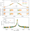 |
Fig. 1 Light curve and model for OGLE-2018-BLG-1126. The anomaly is a dip that is centered at 8298.7, which is detected at ∆χ2 = χ2(1L1S) − χ2(2L1S) = 69. As in all 10 light-curve figures in this paper, we show the full light curve and anomaly region in separate panels, we show the caustic topologies in one or more insets, we show residual panels for indicated models, and we color the data points by observatory, as indicated in the legend. |
Light curve parameters for OGLE-2018-BLG-1126.
3.3 KMT-2018-BLG-2004
The anomaly in Fig. 2 consists of a short bump, which is traced by both KMTS and KMTC data, centered on tanom = 8242.7, when the Moon was about 10° north of the event. While in this case, the Moon was 4 days past full (so the background at passage was 5000, compared to 13 000 for OGLE-2018-BLG-1126), it is far more plausible that the Moon would cause a bump in the light curve, rather than a dip. Indeed, given that the bump is continuous across two observatories separated by 8000 km, it is difficult to conceive of any other source of systematics. However, we again carefully examine the subtracted images and find no evidence of bleeding columns. Hence, we again conclude that the anomaly is due to microlensing.
Using the above tanom, combined with the 1L1S parameters (t0, u0, tE) = (8239.17,0.23,31 day), the heuristic formalism (see Eq. (3)) predicts  and α = 244°. The grid search returns only two solutions, which after refinement agree quite well with these predictions (see Table 3). In particular,
  . The anomaly is detected at χ2(1L1S) − χ2(2L1S) = 167.
Given that the anomaly is a featureless bump, it is essential to check whether it can be explained by a binary source (1L2S) model. From Table 3, we see that such models are disfavored by Δχ2 = 14.8, which is substantial, though not overwhelming, evidence in favor of 2L1S.
In the 1L2S model, the best fit value of the flux ratio is qF = 2.2 × 10⁻³, corresponding to a magnitude difference of ΔI = −2.5log(qF) = 6.6 magnitudes. We show in Sect. 4.2 that the source lies about 3.6 mag below the clump. Hence, the putative source companion would have an absolute magnitude of MI,comp ~ 10. Such stars are common, so the 1L2S solution cannot be regarded as implausible on these grounds.
The 1L2S model makes the definite prediction that the “bump” should be basically invisible in the V band. That is, the source companion should have (V − I)comp,0 ~ 3.3 whereas (as we show in Sect. 4.2), (V − I)S,0 ~ 0.7. Thus, the relative amplitude of the bump should be 100.4(3.3−0.7) = 11 times smaller in V than I. This implies that the V-band light curve should follow the I-band light curve for 2L1S but should follow the 1L1S curve for 1L2S (see Hwang et al. 2018b). Unfortunately, the V data are not good enough to test this prediction. Of the four potential data sets, (KMTC & KMTS) × (BLG01 & BLG41), only KMTS BLG01 provides useful information. This has only one V-band point over the bump. The point lies almost exactly on the 2L1S curve. However, it is only 0.5 σ from the 1L1S curve, due to the relative large V-band error bars.
Thus, the only strong argument against the 1L2S solution is that Δχ2 = 14.8. (If we incorporate the V-band test, just mentioned, this becomes Δχ2 = 15.1). We consider that the planet solution is strongly preferred, but we cannot rule out the binary-source solution unconditionally.
The event is moderately long and has good photometry, so we attempt to fit it for parallax. Figure 3 shows the parallax contours for two of the four cases, namely the “inner” solution with u0 > 0, and u0 < 0.
The parallax fit reveals interesting information. The basic form is of a so-called 1-dimensional (1-D) parallax measurement, which occurs because Earth’s acceleration toward the projected position of the Sun (ψ⊙ = 96.7° north though east) is roughly constant over the relatively short duration of the event (see Sect. 3.1). Formally the error ellipses have an aspect ratio of ~12. The two “lobes” toward the north and south imply that the measurement is subject to the so-called jerk-parallax degeneracy (Gould 2004; Park et al. 2004). While these are striking to the eye, in part because of their large values, πE ~ 2, they are favored by only Δχ2 ~ 4, which would have marginal statistical significance even if the errors could be treated as Gaussian. That is, even in this case, their weight would be overwhelmed by the Galactic priors in a Bayesian analysis, which heavily disfavors such large parallax values. Moreover, in addition to having larger statistical errors along the long axis of the ellipse, the result is also more subject to systematic errors because the information is coming primarily from the wings of the light curve (Smith et al. 2003; Gould 2004).
The actual information in these contours comes from their small width, not their best-fit values. In principle, if these narrow contours were displaced from the origin, as in the first microlensing planet with such features, OGLE-2005-BLG-071 (Dong et al. 2009a), then they would be strong evidence for a minimum value πE ≥ πE,‖, even if the exact value was not determined. However, in the present case, the contours pass through the origin, so the result has less discriminatory value.
Nevertheless, we proceed to extract the essence of the parallax information, while suppressing possible systematic effects, by retaining the short-axis information σ(πE,‖), while setting σ(πE,⊥) → ∞, and using the fact that the contours pass through the origin. Noting that the contours “bend” at the origin, we adopt for the four cases (sgn(u0) = ±;sgn(πEN) = ±), (sgn(u0), sgn(πE,N), σ(πE,‖), ψ) = (+, +, 0.0453,94.29°), (+, −, 0.0482, 104.87°), (−, +, 0.0509, 89.17°), and (−, −, 0.0446,99.76°). Then, when applying Eq. (10) in Sect. 5.2, we evaluate the inverse covariance matrix b in the (north, east) equatorial system as
![Mathematical equation: $ b\left( {N,E} \right) = {1 \over {{{\left[ {\sigma \left( {{\pi _{{\rm{E,}}\parallel }}} \right)} \right]}^2}}}\left( {\matrix{ {_{\sin \psi \,\cos \psi }^{{{\cos }^2}\psi }} & {_{{{\sin }^2}\psi }^{\sin \psi \,\cos \psi }} \cr } } \right) $](/articles/aa/full_html/2022/08/aa43744-22/aa43744-22-eq27.png) (11)
(11)
and we set πE,0 = 0. Because this is a 1-D constraint (albeit on a 2-D space), we substitute  . Note that, by construction, b is a degenerate matrix.
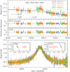 |
Fig. 2 Light curve and model for KMT-2018-BLG-2004. The anomaly is a bump centered at 8242.7. The planetary interpretation is favored over the binary-source model by Δχ2 = χ2(1L2S) − χ2(2L1S) = 14.8. By including V-band data, this becomes Δχ2 = 15.1. |
Light curve parameters for KMT-2018-BLG-2004.
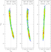 |
Fig. 3 Parallax contours for KMT-2018-BLG-2004 and OGLE-2018-BLG-1367. For both events, these contours have very large axis ratios that are characteristic of so-called 1-D parallax measurements. We argue in the text that only the short-axis information in these contours is reliable and reduce them to truly 1-D constraints (see Eqs. (10) and (11) and Sects. 3.3 and 3.5). |
3.4 OGLE-2018-BLG-1647
Figure 4 shows a pronounced bump Δτ = −0.083 before the peak. The grid search returns two local minima, whose refinements are shown in Table 4. Traditionally, this would be interpreted as the close-wide degeneracy in which the source passes similar-looking central caustics (Fig. 4), for which we would expect the geometric mean to be unity, compared  , for these two reported solutions. On the other hand, adopting u0 = 0.105, the heuristic analysis of Sect. 3.1 yields α = −52° and
  , that is, essentially identical to the geometric mean. Hence, this event is much closer mathematically to the inner-outer degeneracy (derived in the limit of planetary caustics) than it is to the close/wide degeneracy (derived in the limit of central and planetary caustics).
Note that the arithmetic mean of Eq. (2) would yield (s+ + s−)/2 = 1.11. As we discussed in some detail in Sect. 3.1, it was the fact that the geometric mean worked better than the arithmetic mean that led us to adopt Eq. (3) to unify the inner-outer and close-wide degeneracies.
Because the wide-inner model is preferred by Δχ2 = 17, we adopt it over the close-outer model. In any case, the two models have essentially identical mass ratios, q ≃ 0.010. We also search for 1L2S models, but find that they are disfavored by Δχ2 = 28 (see Table 4). Hence, they are decisively rejected.
Due to the faintness of the source, we do not attempt a parallax analysis.
OGLE-2018-BLG-1647 is one of three previously known planets that are listed by Hwang et al. (2022) as “in preparation” but are analyzed here for the first time.
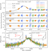 |
Fig. 4 Light curve and model for OGLE-2018-BLG-1647. The anomaly is a bump centered at 8369.2. The planetary interpretation is favored over the binary-source model by Δχ2 = χ2(1L2S) − χ2(2L1S) = 28. While both close and wide caustic structures are illustrated, the wide solution is decisively favored by Δχ2 = 17. Nevertheless, this (albeit broken) degeneracy proved to be the “Rosetta Stone” for the unification of the close/wide and inner-outer degeneracies (see Sects. 3.1 and 3.4). |
Light curve parameters for OGLE-2018-BLG-1647.
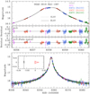 |
Fig. 5 Light curve and model for OGLE-2018-BLG-1367. The anomaly is a flattening of the peak. Such flattened peaks can be produced by finite-source effects in 1L1S events. However, in this case, the 2L1S interpretation is favored by Δχ2 = 65. |
3.5 OGLE-2018-BLG-1367
Figure 5 shows a flattened, or perhaps slightly depressed peak. A natural way to produce a flattened peak is a 1l1S geometry with finite source effects as the lens transits the face of the source, that is, so-called finite-source/point-lens (FSPL) events. We search for such a model, but it produces a relatively poor fit, χ2 (FSPL) −χ2(2L1S) = 65. In addition, the FSPL fit parameters (tE,ρ) = (22.0day, 0.048), would imply an extraordinarily long source self-crossing time (t* = 1.1 day), given that the source is a turnoff star (see Sect. 4.4). Hence, the Einstein radius would be θΕ ≃ 16 μas, while the proper motion would be an extraordinarily slow µrel ≃ 0.27 mas yr−1, with prior probability p = 8 × 10⁻⁵ (see Eq. (14), below). That is, we expect only about one event with such a low proper motion during the five years of KMT normal observations, and this one event would have only a few percent chance of giving rise to finite-source effects (thus enabling its low µrel to come to our attention).
By contrast, the 2L1S models (Table 5) fit the data quite well and do not require exceptional physical parameters. The flattening (or depression) near the peak is then explained by the source passing roughly perpendicular to the planet-host axis on the opposite side of the planet, a region that is characterized by a negative magnification deviation relative to 1L1S.
For perpendicular trajectories,  . Hence, the geometric mean of the two solutions (0.981) is slightly closer to this value than it is to unity (the close-wide prediction). This tends to confirm our conjecture that Eq. (4) is the correct generalization of the s† formalism, even though the event is qualitatively well described by the “close-wide” degeneracy
This is another massive planet, q ≃ 3.4 × 10⁻³, that is, 3.5 times larger than the Jupiter/Sun ratio.
Because the source is relatively bright and the photometry is good, we attempt to measure πΕ. Figure 3 shows the parallax contours for one of the four solutions, namely the close solution for u0 > 0. As in the case of KMT-2018-BLG-2004, the contours are highly elongated (1-D parallax) with two lobes, indicating that the event is subject to the jerk-parallax degeneracy. However, contrary to that case, the contours do not pass through the origin, but rather cross the πE,N axis at πE,E ≃ 0.165, which is 4 times larger than the error. Hence, this parallax measurement contains significant information.
To extract this information, we follow similar procedures to those of Sect. 3.3, but with some difference. First, contrary to the previous case, there is essentially no bend between the positive and negative πE,N regimes. Second, the contours are essentially identical for positive and negative u0. Third, as mentioned above, the contours do not pass through the origin. The first two of these imply that there is one regime: (σ(πE,‖), ψ) = (0.0396,87.30°). To implement the third within the framework of Eq. (10), we rotated the measured πE,‖,0 = 0.165 to Equatorial coordinates:
 (12)
(12)
Light curve parameters for OGLE-2018-BLG-1367.
3.6 OGLE-2018-BLG-1544
Figure 6 shows a dip starting near the peak, followed by a bump centered at tbump = 8352.7. If the latter is attributed to the source crossing the planet-host axis on the planet side, then the heuristic formalism gives α = 208° and  1.03. The angle, in particular, implies that the dip is generated by passage along one of the long sides of the central caustic due to a low-mass (but not necessarily planetary) companion. In principle, there might be other geometries.
However, the grid search finds only two local minima, which correspond to the close and wide versions of the one anticipated above, with q = 0.019 and q = 0.016, respectively, the former being favored by Δχ2 = 3 (see Table 6). Hence, this is another very massive planet (under the planet definition q < 0.03).
Due to the faintness of the source, we do not attempt a parallax analysis.
Because this event has a major-image “bump generating” caustic topology, and despite the fact that it does not exhibit the classical “isolated bump” morphology that would normally induce concerns about a possible binary-source interpretation, we fit for 1L2S models. We find that Δχ2 = χ2(1L2S) − χ2(2L1S) = 5.4 (see Table 6). Hence, while the planetary interpretation is favored, there is a significant possibility that the anomaly is actually due to a binary source.
OGLE-2018-BLG-1544 is one of three previously known planets that are listed by Hwang et al. (2022) as “in preparation” but are analyzed here for the first time.
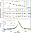 |
Fig. 6 Light curve and model for OGLE-2018-BLG-1544, The anomaly is a long dip near the peak followed by a shorter bump. The heuristic analysis is anchored in the latter, which implies a shallow source trajectory α = 208°. The dip is then understood as the lateral passage of one wall of a central caustic (see inset). |
Light curve parameters for OGLE-2018-BLG-1544.
3.7 OGLE-2018-BLG-0932
OGLE-2018-BLG-0932 is a good example of a case for which the heuristic formalism gives relatively imprecise guidance. The 1L1S approximation has (t0, u0, tE) ≃ (8301.1,0.85,27 day), and tanom ≃ 8273.5, that is, τanom = −1.02. These imply  and α+ = 320° (or α− = 140°). The fact that the anomaly is a “bump” rather than a “dip” leads one to expect that this is major image perturbation, so s† ~ 1.86, α = 320°. In fact, however, a full grid search shows that there is only one solution, for which the bump is due to the source transiting a triangular caustic from a minor-image perturbation and for which the heuristic prediction is
  , α = 140°. Comparison to Table 7 shows that
  , as expected for cases with no inner-outer degeneracy. However, α differs from the prediction by 5°, which is much larger than any of the other cases examined here or the 11 cases to which the heuristic analysis was systematically applied by Hwang et al. (2022) and Ryu et al. (2022). The reason is that the heuristic analysis implicitly assumes that the anomaly is centered on the planet-host axis. This basically holds for major-image planetary perturbations, for dip-like minor-image planetary perturbations, and even for minor-image caustic crossings for the cases of very small q (because the caustics are then very close to the minor-image axis). However, for the present case, q ~ 10−3, the caustic is 0.1 Einstein radii from the axis (see Fig. 7), that is, at an angle sin−1 (0.1/uanom) = 4° relative to this axis, which accounts for the “error” in the heuristic prediction.
The results shown in Table 7 have blending fixed to zero, specifically using the baseline source flux as determined by OGLE. A free fit to blending gives fB/fbase = −0.30 ± 0.09, with an improvement Δχ2 = 6.7. For such a bright source, such large negative blending cannot be the result of unmodeled fluxes from unresolved stars. In principle, it could be a statistical fluctuation (Gaussian probability p = 4%), but is more likely due to low-level systematics or source variability, or possibly to unmodeled physical effects, such as parallax.
From the present perspective, we simply impose zero blending, while noting that the parameters do not change much for the negative blending solutions. For example, the value of q rises from 1.19 × 10⁻³ to 1.26 × 10⁻³. We do not investigate parallax solutions here because this event has Spitzer parallax observations under a large program that was outlined by Yee et al. (2015). These will be analyzed elsewhere.
We searched for 1L2S solutions, but find that these are ruled out by Δχ2 = 564.
OGLE-2018-BLG-0932 is one of three previously known planets that are listed by Hwang et al. (2022) as “in preparation” but are analyzed here for the first time.
Light curve parameters for OGLE-2018-BLG-0932.
3.8 OGLE-2018-BLG-1212
The light curve for this event shows a strong asymmetry due to parallax, even when the anomaly is removed. Hence, contrary to our usual procedures, we fit for parallax prior to searching for 2L1S solutions. Both the 1L1S and 2l1S models in Fig. 8 include parallax. We can still carry out a heuristic analysis using the 1L1S parallax-model parameters (t0, u0, tE) = (8393.76,0.014,51 day), together with the midpoint and width of the dip: tanom = 8394.1 and Δtdip = 0.75 day. These yield  , α = 64°, and q = 7 × 10⁻⁴. These should be compared with the results from the full grid search shown in Table 8, that is,
  , α = 63°, and q = 12 × 10−4.
For the record, we note that in our initial 2L1S fit, we obtained a very well-localized solution at πΕ(Ν, E) = (0.534, 0.550). However, wefound that the jerk-parallax degeneracy formalism (Eqs. (7)–(9) of Park et al. 2004) predicts another solution5 at πΕ(Ν, E) = (−0.404,0.550), and numerical investigation then showed that this was recovered to high precision (see Table 8). While this second set of solutions is disfavored by Δχ2 ~ 11, we keep track of its potential implications because the πE,⊥ (≃ πE,N) parameter is among the most sensitive to subtle systematic errors.
The wide solution is favored by Δχ2 = 3, which is far below the level that would be required to distinguish between the two solutions. However, the parameters (apart from s) of the two solutions are essentially identical.
The very high parallax value πΕ = 0.767, implies a projected velocity  in the geocentric frame. Noting that Earth’s projected velocity at t0 was υ⊕,⊥(Ν, E) = (−2.5, −4.6) km s−1 and adopting υ⊙(l, b) = (12, 7) km s−1 for the peculiar velocity of the Sun relative to the local standard of rest (LSR), this implies
  km s−1 in the Sun frame and
  km s−1 in the LSR frame.
This value tends to favor lens distances Dl ~ 1−2 kpc. That is, ignoring the peculiar motions of the lens relative to the disk and of the source relative to the bulge, ![Mathematical equation: ${{{\bf{\tilde v}}}_{{\rm{lsr}}}}\left( {l,b} \right) \simeq \left[ {{{\left( {{{{D_{\rm{S}}}} \mathord{\left/ {\vphantom {{{D_{\rm{S}}}} {{D_{\rm{L}}} - 1}}} \right. \kern-\nulldelimiterspace} {{D_{\rm{L}}} - 1}}} \right)}^{ - 1}}{v_{{\rm{rot}}}},0} \right]$](/articles/aa/full_html/2022/08/aa43744-22/aa43744-22-eq41.png) for a flat rotation curve with rotation speed υrot = 235 km s−1. This would imply
for a flat rotation curve with rotation speed υrot = 235 km s−1. This would imply  . Because the lens and source peculiar motions cannot truly be ignored, and because there is more phase space at larger distances, this argument is only suggestive. Nevertheless, we discuss its potential implications in Sects. 4.7 and 5.7.
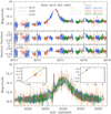 |
Fig. 7 Light curve and model for OGLE-2018-BLG-0932. The anomaly is a bump centered at 8273.5. Unlike most smooth, isolated bumps, this one is due to a source passage over a minor-image caustic, with the smoothness due to the fact that source is very large compared to the caustic (see inset). Among the 10 events analyzed here, this is the only one for which the source-size parameter ρ = θ*/θE is precisely measured. |
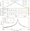 |
Fig. 8 Light curve and model for OGLE-2018-BLG-1212. The anomaly is a dip centered at 8394.1, which is traced by both KMTA and MOA data. The event has a very strong parallax signal and large parallax parameter, πΕ = 0.767 ± 0.019, almost certainly implying a nearby lens (see Sects. 3.8, 4.7, and 5.7). |
3.9 KMT-2018-BLG-2718
From Fig. 9, this event does not, at first sight, appear to be planetary in nature. The anomaly is a dip near the peak of the event, which is of very long duration tdip ~ 20 days. Estimating teff ~ 10 days and  , we can expect6 from Eq. (6) that tq ≃ 2.5 days, so that this event would only meet our planet definition q < qmax = 0.03 provided that tE ≳ tq/qmax ~ 83 days. Nevertheless, the morphology of this very faint (Ipeak ~ 18.7) event does suggest such a long duration. This emphasizes the importance of carefully reviewing all detections of the Anomaly Finder even if they do not look planetary at first sight.
The grid search indeed returns a wide-close pair of planetary solutions with q = 0.020 and q = 0.014 that are in accord with the above heuristic analysis, that is, with timescales tE ~ 160 days and 230 days, respectively. However, it also returns a pair of binary solutions with q ≳ 0.6 (see Table 9). The planetary solutions are favored by Δχ2 = 12.7. If the statistics could be assumed to be Gaussian, then this would decisively resolve the planet/binary ambiguity. However, given the quality of the data and the general inapplicability of Gaussian statistics to microlensing data, we would rather regard this as “basically resolved”.
Due to the faintness of the source, we do not attempt a parallax analysis.
Light curve parameters for OGLE-2018-BLG-1212.
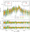 |
Fig. 9 Light curve and model for KMT-2018-BLG-2718. The anomaly is a dip near the peak, which is flanked by two bumps. This morphology is the classic signature of the planet/binary degeneracy identified by Han & Gaudi (2008) (see insets). In this case, the planetary interpretation is favored by Δχ2 = 12.7. The invariant parameter tq = qtE = 3.16 ± 0.16 days would imply non-planetary mass ratios (by our definition, q > 0.03), unless tE ≳ 100 days. In fact, the fits imply much longer timescales (see Table 9). |
 |
Fig. 10 Light curve and model for KMT-2018-BLG-2164. The anomaly is a dip centered at 8290.8. Similar to KMT-2018-BLG-2718, this anomaly is subject to the Han & Gaudi (2008) planet binary degeneracy (see insets), but contrary to that case, the planetary interpretation is not decisively favored (see Table 10). Therefore, the lens companion cannot be claimed as a planet. |
3.10 KMT-2018-BLG-2164
Figure 10 shows a dip near the overall peak, flanked by roughly equal bumps. In principle, this could be caused by the source passing roughly perpendicular to the planet-star axis on the opposite side of the planet, similarly to OGLE-2018-BLG-1367. The grid search indeed returns a close-wide pair that corresponds to this geometry. But it also finds a second pair of minima, in which the source passes diagonally outside a Chang-Refsdal caustic. Refinement of these minima indicate a planet-versus-binary degeneracy, that is, q ~ 0.001 versus q ~ 0.15, which was predicted by Han & Gaudi (2008). The planetary solution is favored by Δχ2 = 3.5, but this is far below the level what would be required to confidently claim a planet (see Table 10). This object is presented here because our protocols demand that we include all companions that are consistent with being planetary, even if this designation cannot be confirmed.
In this case, the planetary and binary solutions predict similar source fluxes and there are no proper-motion estimates (because there is no ρ measurement). Hence, future adaptive optics (AO) observations cannot distinguish between the solutions. This could only be done using RV follow-up observations on extremely large telescopes (ELTs), or possibly even larger telescopes that will operate in the more distant future. Note, however, that even if this proves to be a planet, the uncertainty in log q is 0.2 dex, corresponding to a factor 1.6. This large uncertainty is related to the fact that the improvement relative to 1L1S is only Δχ2 = 89.
Due to the faintness of the source, we do not attempt a parallax analysis.
Light curve parameters for KMT-2018-BLG-2718.
Light curve parameters for KMT-2018-BLG-2164.
3.11 OGLE-2018-BLG-1554
As shown in Fig. 11, the light curve exhibits a long-term deviation over the peak, which is relatively small, but nonetheless we find to be statistically significant at Δχ2 = 413. The grid search returns two pairs of solutions, one being a planetary pair with q ~ 0.025 and the other being a binary pair with q ~ 0.075. In addition to these four solutions, we find a 1L2S solution. All three classes have a member that lies within the overall minimum at Δχ2 < 1.4, so all three are “equally good” in this sense, (see Table 11).
Only the planetary solutions have a ρ measurement, ρ ~ 0.03, corresponding to t* = ρtE ~ 0.4 days. In Sect. 4.10, we show that θ* ≃ 0.93 µas. Hence, if the planetary solution were correct, then µrel = θ*/t* ~ 0.8 mas yr−1. As we explain just below in Sect. 4, the fraction of events with such low proper motions is p < (µrel/6.4masyr−1)3 ≃ 2 × 10⁻³. Thus, we consider the planetary solution to be extremely unlikely.
In any case, given that the planetary solution cannot (at present) be distinguished from the binary-lens and 1L2S solutions, this event cannot be included in (present-day) mass-ratio function studies.
For completeness, we remark that if future AO followup observations confirm the very low µrel ≲ 1mas yr−1 predicted by the planetary solutions, this would constitute strong evidence (though not proof) that it was correct. However, such confirmation would face extreme observational challenges, even with next-generation 30m class telescopes.
The first point is that if the planetary solution is correct, then θE ~ 30 µas, and so πrel ~ 0.11 µas (Μ/ΜΘ)−1. That is, the lens will be invisibly faint unless the lens and source are within  , which is itself highly improbable. Moreover, it means that the “correction” from the measured geocentric to the relevant heliocentric proper motion, Δμ = µrel,hel − µrel = υ⊕⊥ ± πrel/au will be extremely small. Here υ⊕⊥ (Ν, E) = (−3.7, + 13.7) mas yr−1 is the projected velocity of Earth at t0. That is, |Δµ| ~ 0.02(M/0.075 M⊙)−1 mas yr−1, so that µrel,hel − µrel = 0.8 mas yr−1. Given the faintness of the lens, this would require waiting of order 3 decades even with ELTs. Thus, even in the unlikely case that the planetary solution is correct, the prospects for confirming it are distant at best.
Light curve parameters for OGLE-2018-BLG-1554.
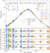 |
Fig. 11 Light curve and model for OGLE-2018-BLG-1554. The anomaly is characterized by weak deviations both before and after the peak. Like the previous two events, this one is subject to the Han & Gaudi (2008) planet/binary degeneracy (see insets), but even more severely (see Table 11). In addition, there is a severe 1L2S/2L1S degeneracy (see Table 11). Therefore, it is not established that the lens has a companion, and even if it does, this companion cannot be claimed as a planet. |
4 Source properties
For a substantial majority of planetary microlensing events that have been reported in the past, ρ was measured. Hence, if the angular source size, θ*, could be determined, it yielded θΕ and µrel:
 (13)
(13)
Then, if πΕ could also be measured, one could directly infer the lens mass and distance via Eq. (8). However, even if πΕ could not be measured, the combination of (tE, θΕ) [so, also, µrel] provided more powerful constraints on the Bayesian mass and distances estimates using Galactic-model priors than is possible from the tE constraint alone. Moreover, the determination of µrel allows one to accurately estimate how long one must wait in order to separately resolve the lens and source in high-resolution follow-up observations using, that is, AO on large telescopes or telescopes in space (for example, Batista et al. 2015; Bennett et al. 2020, 2015).
For this reason, virtually all papers on planetary microlensing events make a serious effort to measure θ*. We follow this general practice here, but we note in advance that, with the exception of two events (OGLE-2018-BLG-1647 and OGLE-2018-BLG-0932), the value of doing so is likely to be minimal. This is because, for all of the other events analyzed here, there are only weak upper limits on ρ, or in some cases no limits at all.
The limit on ρ can be characterized as “weak” if it leads to a “weak” lower limit on the proper motion µlim = θ*/t*lim, where t* = ρtE and t*,lim ≡ ρlimtE. In turn, µlim is “weak” if it does not exclude a significant fraction of the parameter space.
We quantify this as follows. Following the Appendix of Gould et al. (2021), we note that for events with bulge lenses and bulge sources, the fraction of events with µrel < µlim ≪ σ is
 (14)
(14)
where we have modeled the bulge proper-motion distribution as an isotropic Gaussian with dispersion σ = 2.9 mas yr−1. One can show that in this low µlim regime, the probability for disk-bulge lensing is even lower. Thus, for example, if µlim ≲ 0.5 mas yr−1
Notes. (V − I)cl,0 = 1.06. (as in most of our events) then fewer than p ≲ 10−3 of simulated events will be eliminated by imposing this limit, implying negligible impact on the Bayesian estimate.
Nevertheless, while θ* is itself of little use in these cases, the measurements of the source color and magnitude, which are needed to determine θ*, can be important for the interpretation of future AO observations. Together, they will enable prediction of the source flux in the observed band (for example, H or J), and so allow one to determine which of the two stars is the source, with the other being the lens, whose properties will be the main subject of interest. These observations will, by themselves, yield µrel (from the observed separation and elapsed time), and so θE = µreltE. Together with the lens flux, this will enable good estimates of Μ and DL.
Thus, even though these θ* measurements are likely to be of little use, either now or in the future, they are a small additional step relative to the actually necessary color and magnitude measurements. Hence, we report them as well.
Our general approach (with a few exceptions that are explicitly noted) will be to obtain pyDIA (Albrow 2017) reductions of KMT data at one (or possibly several) observatory/field combinations. These yield the microlensing light curve and field-star photometry on the same system. We then determine the source color by regression of the V-band light curve on the I-band light curve, and the source magnitude by regression of the I-band light curve on the best model. We then transform the instrumental KMT photometry to calibrated OGLE photometry, usually OGLE-III (Szymański et al. 2011), but in two cases, OGLE-II (Szymański 2005; Kubiak & Szymański 1997; Udalski et al. 2002). If there is inadequate V-band signal in a single observatory/field, we repeat the procedure for several, check for consistency, and then combine them. In two cases, we are not able to measure (V − I) from the light curve. In one of these cases, we infer the color by combining OGLE-IV I-band observations with H-band observations from the UKIRT microlensing project (Shvartzvald et al. 2017). In the other, we make use of a deep, high-resolution color-magnitude diagram (CMD) based on archival Hubble Space Telescope (HST) data (Holtzman et al. 1998). Figures 12 and 13 show the resulting CMD for each event, with the position of the source and the centroid of the red clump indicated in blue and red respectively. Table 12 lists these values and also shows the steps leading to the calculation of θ* for each event.
For this, we follow the method of Yoo et al. (2004). We adopt the intrinsic color of the clump (V − I)0,cl = 1.06 from Bensby et al. (2013) and its intrinsic magnitude from Table 1 of Nataf et al. (2013). We then obtain [(V − 1), I]s,0 = [(V − 1), I]S + [(V − 1), 1]cl,0 − [(V − I), I]cl. We convert from V/I to V/K using the VIK color-color relations of Bessell & Brett (1988) and then derive θ* from the color/surface-brightness relations of Kervella et al. (2004). After propagating errors, we add 5% in quadrature to account for errors induced by the overall method.
Where relevant, we report the offset of source from the baseline object. In all cases, this is found by comparing the difference image near peak to the baseline object position in the template.
Comments on individual events follow.
CMD parameters.
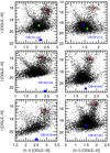 |
Fig. 12 CMDs for 6 of the 10 events analyzed in this paper. The clump centroid is shown in red and the source star is shown in blue. Each panel contains an abbreviation of the event name in blue. Where relevant, we show the blended light in green. |
4.1 OGLE-2018-BLG-1126
The CMD is shown in Fig. 12. There are no useful constraints on ρ. We note that the baseline object has [(V − I), I]base = (2.14,18.70), implying that the blend has [(V − I), I]b = (2.13,18.98), that is, similar in color but about 9 times brighter than the source. We find that it is displaced from the event by 260 mas, meaning that it is almost certainly unrelated to the event. Most likely, it is a bulge subgiant. Its brightness and proximity prevent any useful constraints on the lens flux. On the positive side, it is unlikely to interfere with future AO observations.
4.2 KMT-2018-BLG-2004
The CMD is shown in Fig. 13. The constraints on ρ have practically no impact. The baseline object (Ibase = 18.88) is offset from the source by about 600 mas, meaning that the blend has IB ≃ 19.8 and is almost certainly unrelated to the event. Moreover, the blend color is very poorly determined. Hence, we do not display it in the CMD. We adopt IL > 19.6, which corresponds to IL,0 > 18.1 for bulge lenses (and other lenses that are behind essentially all the dust). This will have a minor effect (see Sect. 5.2).
The magnitude listed in Table 12 is for the planetary solution with the lower χ2, as will always be the case except when otherwise specified. In this case, the other solution would have a larger θ* by 1.4%, that is, a small difference compared to the error bars.
This event is not in the OGLE-III footprint, but fortunately it is in the OGLE-II footprint (Szymański 2005; Kubiak & Szymański 1997; Udalski et al. 2002). As indicated in Fig. 13, we therefore calibrate the photometry using OGLE-II.
4.3 OGLE-2018-BLG-1647
The CMD is shown in Fig. 12. In this case, there are ρ measurements for both solutions. Because the wide solution is favored by Δχ2 = 17, we do not further consider the close solution. While the fractional error in ρ is fairly large (20%), we note that very low values are strongly excluded. For example, ρ > 0.0023 at 2.5 σ, which is very similar to the naive extrapolation from the 1 σ error bar. This corresponds to θΕ < 0.20 mas and µrel < 1.4 mas yr−1 at the same significance. Hence, this is likely to be a low-mass lens in the bulge.
OGLE-III photometry, which resolves out a nearby neighbor at about 600 mas thereby showing a baseline magnitude Ibase = 19.96, implies an estimated blend magnitude IB = 20.57. We set a more conservative limit on the lens brightness IL > 20.30. Given the extinction toward this field, AI = 1.43, this corresponds to IL,0 > 18.87 for lenses that are behind essentially all the dust. Hence, given that the θΕ measurement already favors a low-mass bulge host, the flux constraint plays a limited role. Because we do not have a color determination for the baseline object (hence, also for the blend), we do not display it on the CMD.
4.4 OGLE-2018-BLG-1367
The CMD is shown in Fig. 12. Again, the limit on ρ is very weak, corresponding to θΕ > 0.048 mas and µrel > 0.77 mas yr−1, which are hardly constraining.
OGLE-III shows a baseline magnitude Ibase = 18.57, leaving an estimated blend magnitude IB = 19.92. We set a more conservative limit on the lens brightness IL > 19.70, which corresponds to IL,0 > 18.79 for lenses behind essentially all the dust. This is a very similar, mildly constraining limit as in the case of OGLE-2018-BLG-1647. Again, we do not display the blend on the CMD due to poor color determination.
4.5 OGLE-2018-BLG-1544
The CMD is shown in Fig. 12. The source is blended with a clump giant [(V − I), I]base = (2.88, 16.74), which is separated by 600 mas. Hence, the blended light cannot be constrained. Following the logic that was applied to OGLE-2018-BLG-1647, the limit, ρ < 0.012, implies µrel > 0.45 mas yr−1, which is not useful.
4.6 OGLE-2018-BLG-0932
The CMD is shown in Fig. 13. We are not able to accurately measure the V-band source flux in spite of the source being in or near the clump, for two reasons: the source is heavily reddened and the peak magnification is low (Amax = 1.47). Fortunately, the event lies in the UKIRT microlensing footprint (Shvartzvald et al. 2017), which allows us to determine the source color on an [(I − H), I] CMD. To this end, we match OGLE-IVI and UKIRT H data, which are shown in Fig. 13. We find that the source is Δ(I − H) = −0.016 ± 0.054 bluer than the clump, from which we infer that it is Δ(V − I) = −0.01 ± 0.03, which is the basis of our color determination in Table 12.
Note that for this field, Iogle–iii − IOGLE–IV = 0.04. We do not correct for this offset from standard magnitudes in Table 12. This makes no difference for our estimate of θ*, which depends only on relative photometry. However, it should be noted in the unlikely event that there is future, high-precision, I-band photometry that could probe this level of difference.
Of the 10 events analyzed in this paper, OGLE-2018-BLG-0932 is the only one with a precise ρ measurement and one of only two with any ρ measurement. Combining this with our determination of θ*, we find,
 (15)
(15)
As discussed in Sect. 3.7, the blending is consistent with zero, but is not well measured. We have set fB = 0 in the fit. However, given that the source is a clump giant, we cannot set any useful limits on the lens flux.
4.7 OGLE-2018-BLG-1212
Before evaluating the CMD information for this event, it is important to recall that there is a very precise, and fairly large, parallax measurement πΕ = 0.767 ± 0.019. As discussed in Sect. 3.8, this result strongly favors (but does not prove) that the lens is relatively nearby, that is, only a few kpc from the Sun. In light of this, is notable that the Gaia measurement of the “baseline object”,
 (16)
(16)
suggests that the baseline object may be a very nearby star, or possibly a blend of a nearby object with a more distant star. In particular, one scenario is that this “object” is comprised of a bulge source and a very nearby disk lens (or a companion to the lens). If, for example, the lens contributed half the light (and if the Gaia measurement were not itself corrupted, see below), then the lens should have πL ~ 6 mas. In this case, πrel ≃ πL, in which case the relative proper motion would be µrel = πrel/πEtE ~ (57 mas yr−1)(πrel/6 mas).
Such a high lens-source relative proper motion would have two consequences that are not confirmed. First, the Gaia proper motion itself would be fractionally affected at the same level as the parallax (in this example, by 50%), whereas the actual Gaia proper motion is just ~2 σ from the mean of the bulge distribution. Second, such a high-motion star would be separately resolved in OGLE-II images (from 1999) and would be recognizable either as a “new star” (at position angle ϕ ~ 224°) compared to the OGLE-IV finding chart (from 2010) or as being displaced from the corresponding OGLE-IV object in the same direction. We find no such high proper motion stars in the OGLE-II images.
Thus, while the large Gaia parallax may be suggestive of the presence of a nearby star in the Gaia aperture (whether related to the event of not), it is difficult to infer anything about the lens from this measurement. In addition, we note that Gaia reports a RUWE value of 1.89, probably indicating some form of contamination of the measurement.
Interestingly, OGLE-2018-BLG-1212 was the subject of a Gaia alert, on 2018-10-05 08:38:24, as being a transient of unknown origin. Two of the Gaia points, at HJD′ = 8396.86 and 8396.93, were just 3 days after the anomaly. However, there are only four significantly magnified Gaia points in total. Hence, these data do not help constrain the event.
The CMD is shown in Fig. 12. There are no useful limits on ρ. The OGLE-III baseline object has [(V − I), I]base = (1.50, 18.04), implying [(V − I), I]b = (1.59, 19.16). From its position on the CMD, the blend light could very well be dominated by a companion to the source.
Of more direct interest, the blend light cannot be dominated by the lens. For example, given the parallax measurement πΕ − 0.767, an M = 0.25 M⊙ lens would lie at Dl ~ 0.76 kpc, and so would have roughly IL ~ 19, thus approximately accounting for the IB light. However, after accounting for E(V − I)L ~ 0.4 of reddening, it would have (V − I)L ~ 3.4, implying V ~ 22.4, which is almost 2 magnitudes redder than the blend. On the other hand, if the lens were at Dl ~ 1.5 kpc (as crudely estimated in Sect. 3.8 based on kinematic arguments), then M ~ 0.11 M⊙. In this case, the lens would not contribute significantly to the blended light, thereby avoiding all photometric constraints. In principle, the lens could be farther and so have yet lower mass, but these distances are disfavored by both the declining mass function and the kinematic arguments. These will automatically be taken into account when we carry out a Bayesian analysis in Sect. 5.7.
Thus, in spite of the several intriguing facts about the blend, in the end, its only implication for the analysis is that it places an upper limit on the lens light, for which we adopt IL > 19.0. However, as we discuss in Sect. 5.7, even this role has a relatively modest practical effect.
Finally we note that the proper motion can be expressed µrel = θΕ/tE = κMπe/tE, implying, µrel,hel = 45(M/M⊙)mas yr−1. Hence, if the lens is luminous (M ≳ 0.075 M⊙), then its proper motion is ≳3.3 mas yr−1. Therefore, it will be separated from the source by at least 40 mas by 2030, a plausible first light for AO on ELTs. Note that even if the lens were a white dwarf (WD), it would almost certainly be visible in AO follow-up. For example, at M = 0.6 M⊙, a relatively dim WD with MK = 14, would be at Dl ~ 0.33 kpc and so K ~ 21.6, which would be visible in ELT observations. In this case, the proper motion would be µrel,hel = 27 mas yr−1, so that the separation in 2030 would be ~ 300 mas. Hence, a second epoch would be required for confirmation. Nevertheless, this does mean that a nondetection in ELT AO follow-up would imply that the host is a brown dwarf.
4.8 KMT-2018-BLG-2718
The CMD is shown in Fig. 13. Due to the small variation in the V-band light curve, our standard procedure for determining the source color yields a very imprecise result: (V − I)0,S = 1.54 ± 0.33. We therefore estimate the color from the I-band offset between the source and the clump, which yields (V − I)0,S = 1.37 ± 0.14, using the Galactic bulge CMD derived from HST observation by Holtzman et al. (1998). (As usual, all aspects of this evaluation are based on the lowest-χ2 solution, that is, the planetary solution with s > 1.)
For the four solutions, the limits on ρ shown in Table 9 correspond to t* = (1.6, 1.1, 2.4, 3.1) days. For the second of these, that is, the best fit, this corresponds to µrel > 0.12 mas yr−1. The excluded region contains a fraction  . That is, this limit is completely unconstraining. For the other three cases, the limit is even weaker.
It is unlikely that the ambiguity between planetary and binary solutions can be decisively resolved until RV observations become feasible for this very faint host. Because the planetary solution is formally favored by Δχ2 = 12.7, the event can plausibly be included in mass-ratio function studies. However, this will require a specific decision.
4.9 KMT-2018-BLG-2164
The CMD is shown in Fig. 12. There are no useful constraints on ρ. The OGLE-III baseline object has Ibase = 20.54, yielding Ib = 20.70. We adopt Il > 20.40, corresponding to Il,0 > 18.85 for lenses lying behind essentially all the dust, which is mildly constraining. We remind the reader that there is a factor ~200 ambiguity in q for the two classes of solutions that we presented in Sect. 3.10, which cannot be resolved except by RV observations in the far future. Hence, we believe that this event is unlikely to attract interest for AO follow-up observations.
4.10 OGLE-2018-BLG-1554
The CMD is shown in Fig. 13. As we discussed in Sect. 3.11, there is a ρ measurement only for the planetary solution. We argued that its high value, ρ ≃ 0.03, rendered the planetary solution highly unlikely.
The OGLE-III baseline object has [(V − I), I]base = (2.01, 18.99), which is very similar to the source values from Table 12, [(V − I), I]S = (2.02,19.10), implying that the source is almost unblended. We adopt an upper limit on lens light IL > 22.80, corresponding to IL,0 > 21.17 for lenses lying behind most or all of the dust. This would be a significant constraint. However, because the event is not clearly planetary, this constraint has no practical impact (see Sect. 5.10).
5 Physical Parameters
None of the 10 events reported in this paper have both θE and πE measurements. Hence, as is customary for a substantial majority of microlensing planets, we make Bayesian estimates of the physical parameters of the system by incorporating priors from a Galactic model. In the subsections below, we summarize the constraints that are derived from the light-curve analysis and CMD analysis, as reported in Sects. 3 and 4. Our general approach is to simulate events based on a Galactic model and then assign each event a weight (possibly zero) depending on how well it matches these constraints. For example, if (as is true of several events), the only constraint is the measurement of the Einstein timescale tE ± σ(tE), then the weight of the simulated event i, with timescale tE,i is wi = exp(−χ2/2) where χ2 = (tE − tE,i)2/[σ(tE)]2. The Galactic model is summarized in Sect. 5 of Han et al.(2021b).
In Table 13, we present the resulting Bayesian estimates of the host mass Mhost, the planet mass Mplanet, the distance to the lens system DL, and the planet-host projected separation a⊥. For the majority of events, there are two or more competing solutions. For these cases we show the results of the Bayesian analysis for each solution separately, and we then show the “adopted” values below these. For Mhost, Mplanet, and DL, these are simply the weighted averages of the separate solutions, where the weights are the product of the two factors at the right side of each row. The first factor is simply the total weight from the Bayesian analysis. The second is exp(−Δχ2/2) where Δχ2 is the χ2 difference relative to the best solution (see Ryu et al. 2022). For a⊥, we follow a similar approach provided that either the individual solutions are strongly overlapping or that one solution is strongly dominant. However, if neither condition is met, we enter “bi-modal” instead.
We present Bayesian analyses for 8 of the 10 events, but not for KMT-2018-BLG-2164 and OGLE-2018-BLG-1554 (see Sects. 5.9 and 5.10). Figures 14 and 15 show histograms for Mhost and DL for these 8 events.
5.1 OGLE-2018-BLG-1126
The only constraint is the measurement of tE. As a result the histograms of host mass and distance are extremely broad (see Figs. 14 and 15). The planet has a similarly broad distribution, but is generally in the Neptune-class range. We recall from Sect. 3.2 that the planet is detected by only Δχ2 = 69.
5.2 KMT-2018-BLG-2004
This event has three constraints in addition to the tE measurement. First, there is the 1-D parallax measurement, πE,‖ = 0 ± σ(πE,‖), where the error bar and orientation ψ of the πE,‖ measurement take on four pairs of values that depend on the signs of u0 and πE,N, as given just above Eq. (11). In addition, there are limits on ρ (< 0.021 or < 0.024) and on lens light, Il > 19.60. The 1-D parallax measurement is incorporated via Eqs. (10) and (11) as described in Sect. 3.3. The ρ constraint implies θE ≳ 35 µas, corresponding to µrel ≳ 0.4 mas yr−1, and hence it plays virtually no role. The main information comes from the πE,‖ measurement. Because this measurement is consistent with πE ~ 0, bulge lenses are permitted. Of course, the contours extend up into the north east quadrant of the πE diagram, which is preferred by disk lenses, so these are also permitted. However, because the parallax constraint has constant width, it is more restrictive of disk lenses (which have higher πE) than bulge lenses. Hence, bulge lenses, which are already favored by higher phase-space density, receive a further boost. Within this context the flux constraint plays a modest secondary role by eliminating some bulge lenses at the very top of the main sequence. The planet has a Saturn-class mass, and the system is very likely in, or at least close to, the bulge.
5.3 OGLE-2018-BLG-1647
The wide solution is favored by Δχ2 = 17, so we consider the close-wide degeneracy to be resolved, and so we only show one solution in Table 13. Both tE and ρ are measured from the light curve, and so tE and θE = θ* /ρ enter as constraints (Tables 4 and 12). For the latter we adopt θE = 91 ± 18 µas. Although the error in this measurement is large, θE is nevertheless constrained to be much smaller than in typical events, which strongly favors a low mass Mhost ~ 0.1 Μ⊙ host in or near the Galactic bulge (see Figs. 14 and 15). Hence, despite its high mass ratio, q ≃ 10−2, the planet is likely to be of Jovian mass. We also incorporate the limit on lens light, IL > 20.30 from Sect. 4.3. However, this plays only a small role because the θE measurement already heavily disfavors lenses that are this bright.
5.4 OGLE-2018-BLG-1367
Similar to KMT-2018-BLG-2004, this event has three constraints in addition to the tE measurement. There is 1-D parallax measurement, πE,‖ = 0.165 ± 0.040, as well as limits on ρ < 0.016 and on lens light IL > 19.70. The 1-D parallax measurement is incorporated via Eqs. (10) and (11) with ψ = 87.30°, as described in Sect. 3.5. The ρ constraint implies θE > 48 µas, corresponding to µrel > 0.8 mas yr−1, and hence it plays almost no role. The main information comes from the | | measurement. First, it implies πE > πE,‖ ≃ 0.165, so if the lens is in the bulge (πrel ≲ 10 µas), then Μ =  , which greatly reduces the phase space accessible to bugle lenses. Second, the smallest values of πE are in the north east quadrant of the πE diagram, which is the preferred location of disk lenses. Hence, the lens distance distribution broadly peaks in the disk at DL ~ 5 kpc (that is, πrel ~ 120 µas) and so at masses
  . The flux constraint therefore plays a relatively minor role because lenses that would violate it are already heavily disfavored. The planet is again Jovian class.
Physical properties.
5.5 OGLE-2018-BLG-1544
Nominally, this event has two constraints, a tE measurement and an upper limit on ρ. However, the latter leads to a very weak proper-motion constraint µrel ≳ 0.4 mas yr−1, which therefore plays virtually no role. As with OGLE-2018-BLG-1126 (which has only a tE measurement), the posterior Bayesian distributions of mass and distance are extremely broad. However, because tE is smaller in the present case by a factor ~0.65, these distributions are shifted to somewhat lower mass and distances (see Figs. 14 and 15). Because of the event’s high mass ratio, q ≳ 0.01, the planet mass estimate is centered near the planet-BD boundary, but with a wide dispersion.
5.6 OGLE-2018-BLG-0932
In addition to the tE measurement, this event has two constraints, a measurement of ρ (leading to measurements of θΕ = 0.458 ± 0033 mas and µrel = 6.22 ± 0.44mas yr−1), and a Gaia measurement of the source proper motion µS(N, E) = (−7.53, −8.81) ± (0.17, 0.26) mas yr−1. There are also Spitzer microlensing data for this event, which should ultimately yield a πΕ measurement. However, the analysis of these data is beyond the scope of the present work and will be presented elsewhere.
We note that in Galactic coordinates, the source proper motion is µS(l, b) = (−10.96, +3.78) mas yr−1, which is ~6.2 mas yr−1 from the bulge mean, that is, slightly more than 2 σ and tending in the direction of antirotation. This means that a bulge lens would be expected to generate µrel ~ 7 mas yr−1 (quite consistent with what is observed), while disk lenses would be expected to generate µrel ~ 11 mas yr−1. Thus, the Gaia measurement increases the likelihood of bulge lenses, which are already strongly favored by phase-space considerations. The net result can be judged from Figs. 14 and 15. The planet is in inferred to have Jovian mass.
It will be interesting to compare the host mass estimate in Table 13 to the results of from the future Spitzer analysis. Roughly speaking, Μ ≃ 0.72 ± 0.27 Μ⊙ corresponds to πE = θE,/κΜ = 0.078 ± 0.029.
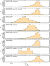 |
Fig. 14 Bayesian estimates of Mhost for the 8 events shown in Table 13. Where there are several solutions, we show the distribution for the one with the lowest χ2. However, as can be assessed from the Table 13, the other solutions hardly differ. |
5.7 OGLE-2018-BLG-1212
For this event, there are two constraints in addition to the tE measurement. First, there is a very well-localized parallax measurement, πE = 0.767 ± 0.019, whose direction (in the LSR frame) is closely aligned to Galactic rotation, that is, 2° ± 1°. Second, there is a limit on lens flux, IL > 19.0.
Table 13 shows that the Bayesian mass and distance estimates are in good accord with the expectations outlined in Sect. 3.8, which was based purely on kinematic arguments. For comparison, we conducted a separate Bayesian analysis in which the flux constraint was ignored. This test showed that inclusion of the flux constraint drove the distance down from 1.62 kpc to 1.55 kpc, that is, a small effect.
We also show in Table 13 the results from the alternate jerk-parallax solutions. These have almost no formal statistical weight, as indicated by the last two columns. The main point is to show that the principal implications for the host and planet masses, the system distance, and the projected separation are not qualitatively different. In particular, the planet is a Saturn-class object that is at 1–2 kpc, orbiting a late M dwarf. As discussed in Sect. 4.7, these predictions can be tested at first AO light on ELTs.
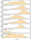 |
Fig. 15 Bayesian estimates of DL for the 8 events shown in Table 13. Where there are several solutions, we show the distribution for the one with the lowest χ2. However, as can be assessed from the Table 13, the other solutions hardly differ. |
5.8 KMT-2018-BLG-2718
Beyond the tE measurement that is common to all events, there is only a weak constraint on the normalized source size, ρ < 0.0068, which leads to an exceedingly weak limit on the proper motion, µrel ≳ 0.1 mas yr−1. Thus, the only real information from the photometric light curve is that the Einstein timescale is exceptionally long. Lenses essentially anywhere along the line of sight can generate such long timescale events by virtue of the rare chance that the source and lens proper motions are very similar. At any distance, large masses  are favored, and these general remarks are well reflected in the distributions shown in Figs. 14 and 15.
5.9 KMT-2018-BLG-2164
KMT-2018-BLG-2164 is neither unambiguously planetary in nature nor is the planetary interpretation significantly preferred. That is, it has only Δχ2 = 4.7 relative to the binary interpretation. Even if Gaussian statistics applied, the binary probability would be ~10%. Therefore, it should not be “registered as a planet” in community databases, and we therefore refrain from trying to characterize it using Bayesian estimates. It is included in the present study only for completeness, that is, to identify all events with viable planetary solutions, regardless of whether these are unique.
5.10 OGLE-2018-BLG-1554
The case for a planetary interpretation for OGLE-2018-BLG-1554 is even weaker than for KMT-2018-BLG-2164. First, the 1L2S solution is slightly preferred by χ2. Second, there is a competing binary solution at Δχ2 ≃ 0. Third, as we remarked in Sect. 4.10, the measured θΕ and µrel for the planetary (but not binary or 1L2S) solution are highly unlikely a priori. Again, this event is only included in this study for completeness. We again counsel against its “registration” as a planet in community databases, and so we refrain from a Bayesian characterization.
6 Conclusions
The goal of this paper was to complete the analysis of all events from 2018 with viable planetary solutions that were identified by the KMTNet AnomalyFinder system and that lie in one or more of the 6 KMT prime fields. Because the main motivation was to prepare a complete sample for statistical analysis, we pushed the boundaries of this sample beyond what will ultimately be used in such studies, and we provide sufficient information to permit future workers to set their own detailed boundaries. In particular, we report on all events with viable solutions with mass ratios q < 0.06, and we provide detailed analysis of all events that have viable solutions with q < 0.03, even for cases that would not normally be published due to ambiguity with binary-lens (q > 0.03) and/or binary-source (1L2S) solutions. Indeed, two of the 10 events that we have analyzed are in one or both of the last two categories and would not normally be published. Of the remaining 8 events, two (OGLE-2018-BLG-1544 and KMT-2018-BLG-2004) have Δχ2 = χ2(1L2S) − χ2(2L1S) = 5.45 and 15.1, respectively, while another (OGLE-2018-BLG-1126) has almost a factor 2 uncertainty in q, which could lead to their exclusion from future statistical studies. Of the other 5 planetary events, 2 (OGLE-2018-BLG-0932 and OGLE-2018-BLG-1647) were previously known, while the remaining 3 (KMT-2018-BLG-2718, OGLE-2018-BLG-1212, and OGLE-2018-BLG-1367) are new discoveries by AlertFinder. These are in addition to the 4 new AlertFinder discoveries that were previously published (OGLE-2018-BLG-0383, OGLE-2018-BLG-0506, OGLE-2018-BLG-0516, and OGLE-2018-BLG-0977). There is one additional AlertFinder recovery, OGLE-2018-BLG-0100, that remains in preparation, but this has an ambiguous mass ratio q at the factor 100 level.
Table 14 shows the 26 events with viable planetary solutions that were recovered or discovered by AnomalyFinder from the 2018 KMT prime-field events. The four previously published discoveries are from Hwang et al. (2022) and Wang et al. (2022). References are given for the 11 previously published recoveries. Note that among these, OGLE-2018-BLG-1700 is marked as a planet in a binary system because the statistical properties of AnomalyFinder discoveries/recoveries may differ for such systems. The 10 entries marked “This work” include seven discoveries and three recoveries, while one previously known planetary solution remains “in preparation”. We consider that the three entries below the line are unlikely to enter a mass-ratio function analysis, while five others (OGLE-2018-BLG-1126, KMT-2018-BLG-1025, KMT-2018-BLG-2004, OGLE-2018-BLG-1700, and OGLE-2018-BLG-1544) will require detailed assessments. Here, we provide only the information necessary for these assessments but not the assessments themselves. All of the events above the line should be entered in planet databases, with names such as OGLE-2018-BLG-1126Lb, and none of the events below the line should be so entered. That is, while OGLE-2018-BLG-0100 is almost certainly planetary in nature, its degeneracies have not yet been delineated in published form, while the other two events below the line are not unambiguously planetary.
Through the course of our systematic study of the 10 events published here, we noticed that the “s†” formalism that was introduced by Hwang et al. (2022) for heuristic analysis should be slightly modified, from using the arithmetic to the geometric mean of the two solutions. In this form, it unifies the so-called close-wide degeneracy of Griest & Safizadeh (1998) for central and resonant caustics with the so-called inner-outer degeneracy of Gaudi & Gould (1997) for planetary caustics, a unification that was previously conjectured by Yee et al. (2021).
AnomalyFinder planets in KMT prime fields for 2018.
Acknowledgements
This research has made use of the KMTNet system operated by the Korea Astronomy and Space Science Institute (KASI) and the data were obtained at three host sites of CTIO in Chile, SAAO in South Africa, and SSO in Australia. Work by C.H. was supported by the grants of National Research Foundation of Korea (2020R1A4A2002885 and 2019R1A2C2085965). W.Z. and H.Y. acknowledge support by the National Science Foundation of China (Grant No. 12133005). The MOA project is supported by JSPS KAKENHI Grant No. JSPS24253004, JSPS26247023, JSPS23340064, JSPS15H00781, JP16H06287, and JP17H02871. UKIRT is currently owned by the University of Hawaii (UH) and operated by the UH Institute for Astronomy; operations are enabled through the cooperation of the East Asian Observatory. The collection of the 2018 data reported here was supported by NASA grant NNG16PJ32C and JPL proposal #18-NUP2018-0016. This paper makes use of data from the UKIRT microlensing surveys (Shvartzvald et al. 2017) provided by the UKIRT Microlensing Team and services at the NASA Exoplanet Archive, which is operated by the California Institute of Technology, under contract with the National Aeronautics and Space Administration under the Exoplanet Exploration Program.
References
- Alard, C., & Lupton, R. H. 1998, ApJ, 503, 325 [Google Scholar]
- Albrow, M. D. 2017, https://doi.org/10.5281/zenodo.268049 [Google Scholar]
- Albrow, M. D., Horne, K., Bramich, D. M., et al. 2009, MNRAS, 397, 2099 [NASA ADS] [CrossRef] [Google Scholar]
- An, J. H., Albrow, M. D., Beaulieu, J.-P., et al. 2002, ApJ, 572, 521 [NASA ADS] [CrossRef] [Google Scholar]
- Batista, V., Gould, A., Dieters, S., et al. 2011, A&A, 529, A102 [NASA ADS] [CrossRef] [EDP Sciences] [Google Scholar]
- Batista, V., Beaulieu, J.-P., Bennett, D. P., et al. 2015, ApJ, 808, 170 [Google Scholar]
- Bennett, D. P., Bhattacharya, A., Anderson, J., et al. 2015, ApJ, 808, 169 [Google Scholar]
- Bennett, D. P., Bhattacharya, A., Beaulieu, J. P., et al. 2020, AJ, 159, 68 [NASA ADS] [CrossRef] [Google Scholar]
- Bensby, T., Yee, J. C., Feltzing, S., et al. 2013, A&A, 549, A147 [NASA ADS] [CrossRef] [EDP Sciences] [Google Scholar]
- Bessell, M. S., & Brett, J. M. 1988, PASP, 100, 1134 [Google Scholar]
- Bond, I. A., Abe, F., Dodd, R. J., et al. 2001, MNRAS, 327, 868 [Google Scholar]
- Calchi Novati, S., Suzuki, D., Udalski, A., et al. 2019, AJ, 157, 121 [Google Scholar]
- Cassan, A., Kubas, D., Beaulieu, J.-P., et al. 2012, Nature, 481, 167 [NASA ADS] [CrossRef] [Google Scholar]
- Dominik, M. 1999, A&A, 349, 108 [NASA ADS] [Google Scholar]
- Dong, S., Gould, A., Udalski, A., et al. 2009a, ApJ, 695, 970 [NASA ADS] [CrossRef] [Google Scholar]
- Dong, S., Bond, I. A., Gould, A., et al. 2009b, ApJ, 698, 1826 [Google Scholar]
- Gaudi, B. S. 1998, ApJ, 506, 533 [Google Scholar]
- Gaudi, B. S., & Gould, A. 1997, ApJ, 486, 85 [Google Scholar]
- Gaudi, B. S., Albrow, M. D., An, J., et al. 2002, ApJ, 566, 463 [NASA ADS] [CrossRef] [Google Scholar]
- Gould, A. 1992, ApJ, 392, 442 [Google Scholar]
- Gould, A. 1996, ApJ, 470, 201 [NASA ADS] [CrossRef] [Google Scholar]
- Gould, A. 2000, ApJ, 542, 785 [NASA ADS] [CrossRef] [Google Scholar]
- Gould, A. 2004, ApJ, 606, L319 [CrossRef] [Google Scholar]
- Gould, A., Miralda-Escudé, J., & Bahcall, J. N. 1994, ApJ, 423, L105 [NASA ADS] [CrossRef] [Google Scholar]
- Gould, A., Dong, S., Gaudi, B. S., et al. 2010, ApJ, 720, 1073 [NASA ADS] [CrossRef] [Google Scholar]
- Gould, A., Ryu, Y.-H., Calchi Novati, S., et al. 2020, JKAS, 53, 9 [NASA ADS] [Google Scholar]
- Gould, A., Zang, W., Mao, S., & Dong, S. 2021, RAA, 21, 133 [NASA ADS] [Google Scholar]
- Griest, K., & Safizadeh, N. 1998, ApJ, 500, 37 [Google Scholar]
- Han, C. 2006, ApJ, 638, 1080 [Google Scholar]
- Han, C., & Gaudi, B. S. 2008, ApJ, 689, 53 [CrossRef] [Google Scholar]
- Han, C., Udalski, A., Gould, A., et al. 2016, ApJ, 828, 53 [NASA ADS] [CrossRef] [Google Scholar]
- Han, C., Bennett, D. P., Udalski, A., et al. 2019, AJ, 158, 114 [Google Scholar]
- Han, C., Lee, C.-U., Udalski, A., et al. 2020a, AJ, 159, 48 [Google Scholar]
- Han, C., Shin, I.-G., Jung, Y. K., et al. 2020b, A&A, 641A, 105 [Google Scholar]
- Han, C., Udalski, A., Lee, C.-U., et al. 2021a, A&A, 649, A90 [EDP Sciences] [Google Scholar]
- Han, C., Udalski, A., Kim, D., et al. 2021b, A&A, 655, A21 [NASA ADS] [CrossRef] [EDP Sciences] [Google Scholar]
- Herrera-Martin, A., Albrow, A., Udalski, A., et al. 2020, AJ, 159, 134 [CrossRef] [Google Scholar]
- Hodgkin, S. T., Irwin, M. J., Hewett, P. C., & Warren, S. J. 2009, MNRAS, 394, 675 [CrossRef] [Google Scholar]
- Holtzman, J. A., Watson, A. M., Baum, W. A., et al. 1998, AJ, 115, 1946 [Google Scholar]
- Hwang, K.-H., Choi, J.-Y., Bond, I. A., et al. 2013, ApJ, 778, 55 [Google Scholar]
- Hwang, K.-H., Udalski, A., Shvartzvald, Y., et al. 2018a, AJ, 155, 20 [Google Scholar]
- Hwang, K.-H., Udalski, A., Bond, I. A., et al. 2018b, AJ, 155, 259 [Google Scholar]
- Hwang, K.-H., Zang, W., Gould, A., et al. 2022, AJ, 163, 43 [NASA ADS] [CrossRef] [Google Scholar]
- Irwin, M. J., Lewis, J., Hodgkin, S., et al. 2004, Proc. SPIE, 5493, 411 [Google Scholar]
- Jung, Y. K., Gould, A., Udalski, A., et al. 2019, AJ, 158, 28 [NASA ADS] [CrossRef] [Google Scholar]
- Jung, Y. K., Gould, A., Udalski, A., et al. 2020a, AJ, 160, 148 [NASA ADS] [CrossRef] [Google Scholar]
- Jung, Y. K., Han, C., Udalski, A., et al. 2021, AJ, 161, 293 [NASA ADS] [CrossRef] [Google Scholar]
- Kervella, P., Thévenin, F., Di Folco, E., & Ségransan, D. 2004, A&A, 426, 297 [NASA ADS] [CrossRef] [EDP Sciences] [Google Scholar]
- Kim, S.-L., Lee, C.-U., Park, B.-G., et al. 2016, JKAS, 49, 37 [Google Scholar]
- Kim, D.-J., Kim, H.-W., Hwang, K.-H., et al. 2018a, AJ, 155, 76 [Google Scholar]
- Kim, D.-J., Hwang, K.-H., Shvartzvald, et al. 2018b, AAS J., submitted [arXiv:1806.07545] [Google Scholar]
- Kim, H.-W., Hwang, K.-H., Gould, A., et al. 2021, AJ, 162, 15 [NASA ADS] [CrossRef] [Google Scholar]
- Kondo, I., Yee, J. C., Bennett, D. P., et al. 2021, AJ, 162, 77 [NASA ADS] [CrossRef] [Google Scholar]
- Kubiak, M., & Szymański, M. K. 1997, Acta Astron., 47, 319 [NASA ADS] [Google Scholar]
- Nataf, D. M., Gould, A., Fouqué, P., et al. 2013, ApJ, 769, 88 [Google Scholar]
- Paczyński, B. 1986, ApJ, 304, 1 [NASA ADS] [CrossRef] [Google Scholar]
- Park, B.-G., DePoy, D. L., Gaudi, B. S., et al. 2004, ApJ, 609, 166 [NASA ADS] [CrossRef] [Google Scholar]
- Ryu, Y.-H., Udalski, A., Yee, J. C., et al. 2020, AJ, 160, 183 [Google Scholar]
- Ryu, Y.-H., Mroz, P., Gould, A., et al. 2021, AJ, 161, 126 [NASA ADS] [CrossRef] [Google Scholar]
- Ryu, Y.-H., Jung, Y. K., Yang, H., et al. 2022, AJ, submitted, [arXiv:2202.03022] [Google Scholar]
- Shvartzvald, Y., Maoz, D., Udalski, A., et al. 2016, MNRAS, 457, 4089 [Google Scholar]
- Shvartzvald, Y., Bryden, G., Gould, A., et al. 2017, AJ, 153, 61 [NASA ADS] [CrossRef] [Google Scholar]
- Skowron, J., Udalski, A., Gould, A. et al. 2011, ApJ, 738, 87 [Google Scholar]
- Smith, M., Mao, S., & Paczyński, B., 2003, MNRAS, 339, 925 [NASA ADS] [CrossRef] [Google Scholar]
- Suzuki, D., Bennett, D. P., Sumi, T., et al. 2016, ApJ, 833, 145 [Google Scholar]
- Szymański, M. K. 2005, Acta Astron., 55, 43 [Google Scholar]
- Szymański, M. K., Udalski, A., Soszyński, I., et al. 2011, Acta Astron., 61, 83 [NASA ADS] [Google Scholar]
- Tomaney, A. B., & Crotts, A. P. S. 1996, AJ, 112, 2872 [Google Scholar]
- Udalski, A. 2003, Acta Astron., 53, 291 [NASA ADS] [Google Scholar]
- Udalski, A., Szymański, M., Kaluzny, J., et al. 1994, Acta Astron., 44, 227 [NASA ADS] [Google Scholar]
- Udalski, A., Szymański, M., Kubiak, M. et al., 2002, Acta Astron., 52, 217 [NASA ADS] [Google Scholar]
- Wang, H., Zang, W., Zhu, W., et al. 2022, MNRAS, 510, 1778 [Google Scholar]
- Woźniak, P. R. 2000, Acta Astron., 50, 421 [NASA ADS] [Google Scholar]
- Yee, J. C., Shvartzvald, Y., Gal-Yam, A., et al. 2012, ApJ, 755, 102 [Google Scholar]
- Yee, J. C., Gould, A., & Beichman, C. 2015, ApJ, 810, 155 [NASA ADS] [CrossRef] [Google Scholar]
- Yee, J. C., Zang, W., Udalski, A., et al. 2021, AJ, 162, 180 [NASA ADS] [CrossRef] [Google Scholar]
- Yoo, J., DePoy, D. L., Gal-Yam, A., et al. 2004, ApJ, 603, 139 [Google Scholar]
- Zang, W., Han, C., Kondo, I., et al. 2021a, RAA, 21, 739 [NASA ADS] [Google Scholar]
- Zang, W., Hwang, K.-H., Udalski, A., et al. 2021b, AJ, 162, 163 [NASA ADS] [CrossRef] [Google Scholar]
- Zang, W., Yang, H., Han, C., et al. 2022, MNRAS, 515, 928 [NASA ADS] [CrossRef] [Google Scholar]
From detailed analysis, the remaining event, OGLE-2018-BLG-0100/KMT-2018-BLG-2296, is known to be planetary in nature but with competitive solutions that differ in q by a factor 100, so that it is not suitable for mass-ratio function studies.
Prior to the work of Herrera-Martin et al. (2020) and Yee et al. (2021), the inner-outer degeneracy was conceived more narrowly as having the source pass on opposite sides of detached planetary caustic(s). To our knowledge, there had been only two recognized cases of this degeneracy, that is, OGLE-2016-1067 with minor-image caustics (Calchi Novati et al. 2019) and OGLE-2017-0173 with a major-image caustic (Hwang et al. 2018a).
Note that in the geometric-mean formalism of Eq. (3),  , which conforms to the minor-image caustic morphology of the light curve. However, this is not true of the arithmetic-mean prediction s† = (s+ + s−)/2 > 1, This was a significant puzzle for us when we initially analyzed this event, but was resolved after analyzing the “Rosetta Stone” event OGLE-2018-BLG-1647 (see Sect. 3.1).
The main differences between AnomalyFinder1.0 and Anomaly Finder2.0 concern the handling of so-called bad points. Anomaly Finder1.0 was extremely aggressive in rejecting data with high background and large seeing. However, Zang et al. (2022) found that there was no correlation between background and discrepant data points, and so eliminated this condition. They also found that many large-seeing points contributed to the detection and characterization of anomalies. Hence, they grouped data by seeing as “good”, “ok”, and “bad”, and then renormalized the error bars for each group separately. Before doing so, they followed Kim et al. (2018a) in eliminated the 10% worst outliers to the point-lens fit. See Zang et al. (2022) for further details.
The event peaked almost at quadrature, that is, ψ = 101° in this formalism. Moreover the projected position of the Sun at this time is only 0.2° from due west, implying that πE,⊥ ≃ −πE,N. Thus, to an excellent approximation, Park et al. (2004) Eq. (9) becomes  where β = −4.76° is the ecliptic latitude. Hence, Eq. (7) becomes
  , very close to the more exact calculation.
The actual value, derived from the MCMCs of both close and wide planetary models is 3.16 ± 0.16 days.
All Tables
All Figures
|
Fig. 1 Light curve and model for OGLE-2018-BLG-1126. The anomaly is a dip that is centered at 8298.7, which is detected at ∆χ2 = χ2(1L1S) − χ2(2L1S) = 69. As in all 10 light-curve figures in this paper, we show the full light curve and anomaly region in separate panels, we show the caustic topologies in one or more insets, we show residual panels for indicated models, and we color the data points by observatory, as indicated in the legend. |
| In the text | |
|
Fig. 2 Light curve and model for KMT-2018-BLG-2004. The anomaly is a bump centered at 8242.7. The planetary interpretation is favored over the binary-source model by Δχ2 = χ2(1L2S) − χ2(2L1S) = 14.8. By including V-band data, this becomes Δχ2 = 15.1. |
| In the text | |
|
Fig. 3 Parallax contours for KMT-2018-BLG-2004 and OGLE-2018-BLG-1367. For both events, these contours have very large axis ratios that are characteristic of so-called 1-D parallax measurements. We argue in the text that only the short-axis information in these contours is reliable and reduce them to truly 1-D constraints (see Eqs. (10) and (11) and Sects. 3.3 and 3.5). |
| In the text | |
|
Fig. 4 Light curve and model for OGLE-2018-BLG-1647. The anomaly is a bump centered at 8369.2. The planetary interpretation is favored over the binary-source model by Δχ2 = χ2(1L2S) − χ2(2L1S) = 28. While both close and wide caustic structures are illustrated, the wide solution is decisively favored by Δχ2 = 17. Nevertheless, this (albeit broken) degeneracy proved to be the “Rosetta Stone” for the unification of the close/wide and inner-outer degeneracies (see Sects. 3.1 and 3.4). |
| In the text | |
|
Fig. 5 Light curve and model for OGLE-2018-BLG-1367. The anomaly is a flattening of the peak. Such flattened peaks can be produced by finite-source effects in 1L1S events. However, in this case, the 2L1S interpretation is favored by Δχ2 = 65. |
| In the text | |
|
Fig. 6 Light curve and model for OGLE-2018-BLG-1544, The anomaly is a long dip near the peak followed by a shorter bump. The heuristic analysis is anchored in the latter, which implies a shallow source trajectory α = 208°. The dip is then understood as the lateral passage of one wall of a central caustic (see inset). |
| In the text | |
|
Fig. 7 Light curve and model for OGLE-2018-BLG-0932. The anomaly is a bump centered at 8273.5. Unlike most smooth, isolated bumps, this one is due to a source passage over a minor-image caustic, with the smoothness due to the fact that source is very large compared to the caustic (see inset). Among the 10 events analyzed here, this is the only one for which the source-size parameter ρ = θ*/θE is precisely measured. |
| In the text | |
|
Fig. 8 Light curve and model for OGLE-2018-BLG-1212. The anomaly is a dip centered at 8394.1, which is traced by both KMTA and MOA data. The event has a very strong parallax signal and large parallax parameter, πΕ = 0.767 ± 0.019, almost certainly implying a nearby lens (see Sects. 3.8, 4.7, and 5.7). |
| In the text | |
|
Fig. 9 Light curve and model for KMT-2018-BLG-2718. The anomaly is a dip near the peak, which is flanked by two bumps. This morphology is the classic signature of the planet/binary degeneracy identified by Han & Gaudi (2008) (see insets). In this case, the planetary interpretation is favored by Δχ2 = 12.7. The invariant parameter tq = qtE = 3.16 ± 0.16 days would imply non-planetary mass ratios (by our definition, q > 0.03), unless tE ≳ 100 days. In fact, the fits imply much longer timescales (see Table 9). |
| In the text | |
|
Fig. 10 Light curve and model for KMT-2018-BLG-2164. The anomaly is a dip centered at 8290.8. Similar to KMT-2018-BLG-2718, this anomaly is subject to the Han & Gaudi (2008) planet binary degeneracy (see insets), but contrary to that case, the planetary interpretation is not decisively favored (see Table 10). Therefore, the lens companion cannot be claimed as a planet. |
| In the text | |
|
Fig. 11 Light curve and model for OGLE-2018-BLG-1554. The anomaly is characterized by weak deviations both before and after the peak. Like the previous two events, this one is subject to the Han & Gaudi (2008) planet/binary degeneracy (see insets), but even more severely (see Table 11). In addition, there is a severe 1L2S/2L1S degeneracy (see Table 11). Therefore, it is not established that the lens has a companion, and even if it does, this companion cannot be claimed as a planet. |
| In the text | |
|
Fig. 12 CMDs for 6 of the 10 events analyzed in this paper. The clump centroid is shown in red and the source star is shown in blue. Each panel contains an abbreviation of the event name in blue. Where relevant, we show the blended light in green. |
| In the text | |
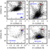 |
Fig. 13 Same as Fig. 12, but for the remaining 4 (out of 10) of the events analyzed in this paper. |
| In the text | |
|
Fig. 14 Bayesian estimates of Mhost for the 8 events shown in Table 13. Where there are several solutions, we show the distribution for the one with the lowest χ2. However, as can be assessed from the Table 13, the other solutions hardly differ. |
| In the text | |
|
Fig. 15 Bayesian estimates of DL for the 8 events shown in Table 13. Where there are several solutions, we show the distribution for the one with the lowest χ2. However, as can be assessed from the Table 13, the other solutions hardly differ. |
| In the text | |
Current usage metrics show cumulative count of Article Views (full-text article views including HTML views, PDF and ePub downloads, according to the available data) and Abstracts Views on Vision4Press platform.
Data correspond to usage on the plateform after 2015. The current usage metrics is available 48-96 hours after online publication and is updated daily on week days.
Initial download of the metrics may take a while.