| Issue |
A&A
Volume 692, December 2024
|
|
|---|---|---|
| Article Number | A106 | |
| Number of page(s) | 8 | |
| Section | Planets, planetary systems, and small bodies | |
| DOI | https://doi.org/10.1051/0004-6361/202451620 | |
| Published online | 05 December 2024 | |
KMT-2024-BLG-1044L: A sub-Uranus microlensing planet around a host at the star–brown dwarf mass boundary
1
Department of Physics, Chungbuk National University,
Cheongju
28644,
Republic of Korea
2
Korea Astronomy and Space Science Institute,
Daejon
34055,
Republic of Korea
3
Max Planck Institute for Astronomy,
Königstuhl 17,
69117
Heidelberg,
Germany
4
Department of Astronomy, The Ohio State University,
140 W. 18th Ave.,
Columbus,
OH
43210,
USA
5
University of Canterbury, Department of Physics and Astronomy,
Private Bag 4800,
Christchurch
8020,
New Zealand
6
Department of Particle Physics and Astrophysics, Weizmann Institute of Science,
Rehovot
76100,
Israel
7
Center for Astrophysics | Harvard & Smithsonian
60 Garden St.,
Cambridge,
MA
02138,
USA
8
Department of Astronomy and Tsinghua Centre for Astrophysics, Tsinghua University,
Beijing
100084,
China
★ Corresponding author; This email address is being protected from spambots. You need JavaScript enabled to view it.
Received:
23
July
2024
Accepted:
2
November
2024
Abstract
Aims. We analysed microlensing data to uncover the nature of the anomaly that appeared near the peak of the short-timescale microlensing event KMT-2024-BLG-1044. Despite the anomaly’s brief duration of less than a day, it was densely observed through high-cadence monitoring conducted by the KMTNet survey.
Methods. Detailed modelling of the light curve confirmed the planetary origin of the anomaly and revealed two possible solutions, due to an inner–outer degeneracy. The two solutions provide different measured planet parameters: (s, q)inner = [1.0883 ± 0.0027, (3.125 ± 0.248) × 10−4] for the inner solutions and (s, q)outer = [1.0327 ± 0.0054, (3.350 ± 0.316) × 10−4] for the outer solutions.
Results. Using Bayesian analysis with constraints provided by the short event timescale (tE ~ 9.1 day) and the small angular Einstein radius (θE ~ 0.16 mas for the inner solution and ~ 0.10 mas for the outer solutio), we determined that the lens is a planetary system consisting of a host near the boundary between a star and a brown dwarf and a planet with a mass lower than that of Uranus. The discovery of the planetary system highlights the crucial role of the microlensing technique in detecting planets that orbit substellar brown dwarfs or very low-mass stars.
Key words: planets and satellites: detection
© The Authors 2024
 Open Access article, published by EDP Sciences, under the terms of the Creative Commons Attribution License (https://creativecommons.org/licenses/by/4.0), which permits unrestricted use, distribution, and reproduction in any medium, provided the original work is properly cited.
This article is published in open access under the Subscribe to Open model. This email address is being protected from spambots. You need JavaScript enabled to view it. to support open access publication.
1 Introduction
Mao & Paczyński (1991) and Gould & Loeb (1992) first pointed out that microlensing could be used as a tool for detecting extrasolar planets. Experimental searches for planets began in the mid-1990s, and the first microlensing planet was detected in 2003 by Bond et al. (2004). To date, 221 microlensing planets have been reported, according to the NASA Exoplanet Archive1. Currently, microlensing ranks as the third most prolific planet detection method, behind the transit and radial velocity methods.
Planetary signals in lensing light curves are typically brief. Consequently, detecting these short-lived signals in microlensing light curves necessitates dense coverage of lensing events. To address this need, early planetary searches combined large-scale survey programmes, such as the Optical Gravitational Lensing Experiment (OGLE; Udalski et al. 1994), the Massive Astrophysical Compact Halo Object survey (MACHO; Alcock et al. 1993), and Microlensing Observations in Astrophysics (MOA; Bond, et al. 2001), with dedicated follow-up observation networks. These follow-up networks included the Galactic Microlensing Alerts Network (GMAN; Alcock et al. 1997), the Probing Lensing Anomalies NETwork (PLANET; Albrow et al. 1998), the Microlensing Follow-Up Network (μFUN; Gould et al. 2006), and RoboNet (Tsapras et al. 2003). In this mode of observations, survey experiments monitored a wide region of the Galactic bulge to detect lensing events, while followup groups utilised multiple narrow-field telescopes to conduct dense observations of the events identified by the surveys. This survey+follow-up strategy only allowed for dense observations of a limited number of events, resulting in fewer than five planetary detections per year before 2010. From 2010 to 2015, the number of detections nearly doubled with a moderate modification to the observational strategy. In the modified mode, follow-up observations were mainly focused on the peak phases of high-magnification events, for which the probability of planet detection is high. Another strategy employed during this period was the auto-follow-up mode. In this approach, when a survey detects a potential anomalous lensing event in progress, an alert is triggered to promptly initiate follow-up observations (Suzuki et al. 2016). A dramatic increase in planet detections occurred with the commencement of high-cadence surveys using multiple telescopes equipped with very wide-field cameras. These surveys significantly increased the number of lensing event detections from several dozen per year to over 3000. With the ability to densely monitor all detected lensing events, the number of planet detections also dramatically increased, and currently an average of 25 planets are being reported annually.
The primary significance of the microlensing technique is its ability to detect planetary systems that might be difficult to identify using other observational methods. While transit and radial velocity methods are sensitive to planets that are close to their host stars, the microlensing method is adept at detecting planets in wide orbits. Additionally, microlensing can identify distant planetary systems located in both the disc and bulge regions of the Galaxy. While planets are typically detected through their effect on their host stars, the microlensing effect can be caused by the planet’s own gravity, enabling the detection of free-floating planets2. Furthermore, because microlensing relies on the gravitational influence of a lensing object, it possesses a unique capability to detect planets belonging to dark or very faint celestial bodies, such as brown dwarfs (BDs), very faint stars, and stellar remnants. A comprehensive discussion of the various advantages of the microlensing method is provided in the review by Gaudi (2012). This capability makes microlensing an invaluable tool for obtaining a comprehensive view of the demographics of planetary systems throughout the Galaxy.
In this study we report the discovery of a low-mass planet orbiting a very low-mass host. The planetary system was discovered from the analysis of a brief anomaly signal in the light curve of the short-timescale lensing event KMT-2024-BLG-1044. Based on the constraints provided by the event timescale together with the angular size of the Einstein ring, it was estimated that the planet has a mass lower than that of Uranus and that the host has a mass at the boundary between BDs and low-mass stars.
2 Observations and data
The lensing event KMT-2024-BLG-1044 was detected by the Korea Microlensing Telescope Network (KMTNet; Kim et al. 2016) survey during the 2024 season using the EventFinder algorithm (Kim et al. 2018). The KMTNet survey operates three identical telescopes strategically positioned in the Southern Hemisphere: the Cerro Tololo Inter-American Observatory in Chile (KMTC), the South African Astronomical Observatory in South Africa (KMTS), and the Siding Spring Observatory in Australia (KMTA). On May 20, 2024 (HJD′ = 450), when the event was detected, the source flux had just passed its peak magnification. Here, HJD′ ≡ HJD – 2 460 000 represents a shortened heliocentric Julian date. The magnitude of the source before the onset of lensing magnification was Ibase = 18.85, and it reached Ipeak = 17.82 at its highest point. The equatorial and Galactic coordinates of the source are (RA, Dec)J2000 =(18: 06:15.36, −27:35:33.29) and (l, b) = (3°.4484,−3°.2509), respectively. The extinction towards the field was AI = 0.98. The source is located in the overlapping region of the KMTNet prime fields BLG03 and BLG43, towards which KMTNet observations were most frequently conducted. The observation cadence was 0.5 hours for each field and 0.25 hours for the combined field. Thanks to this high cadence, the light curve was densely covered despite the relatively short duration of the event.
Figure 1 displays the light curve of the lensing event, compiled from all KMTNet datasets. At first glance, the light curve appears to be that of a typical single-lens single-source (1L1S) event with a smooth and symmetrical shape. However, upon closer examination, a brief anomaly near the peak of the light curve was identified. This anomaly persisted for less than a day, occurring between HJD′ = 449.6 and 449.9. The upper panel provides a magnified view of this anomaly. The primary portion of the anomaly showed a positive deviation from the 1L1S model. Additionally, there were minor negative deviations observed just before and after the main positive deviation.
Initially, the photometry data of the event were processed using the automated KMTNet pipeline, which is based on the pySIS code developed by Albrow et al. (2009). To ensure the data’s optimal quality for analysis, we performed additional photometry using the code developed by Yang et al. (2024). In preparing the data for analysis, we normalised the error bars of the data to achieve consistency with the data scatter and to standardise the degree of freedom to unity for each dataset. This error-bar normalisation procedure followed the protocol outlined in Yee et al. (2012), that is, σ = k(σmin + σ0)1/2, where σmin is a factor used to consider the data scatter, and k is the rescaling factor. Table 1 list the values of σmin and k for the individual datasets. For a subset of the KMTC data, we conducted additional photometry using the pyDIA code (Albrow 2017) for the source colour measurement. The detailed procedure for the source colour determination is described in Sect. 4.
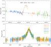 |
Fig. 1 Light curve of the lensing event KMT-2024-BLG-1044. Lower panel: full view of the light curve. Upper panel: zoomed-in view of the peak region around the anomaly. The solid curve drawn over the data points is a single-lens single-source model obtained by fitting the data excluding those around the anomaly. The colours of the data points correspond to those of the datasets marked in the legend. |
Factors used for error-bar normalisation.
3 Lensing light curve analysis
The pattern of the anomaly observed in the light curve of KMT-2024-BLG-1044 offers several crucial clues about its origin. Firstly, the rapid rise and fall of the source flux during the main feature of the anomaly suggest that it was likely caused by the source crossing a caustic created by a companion to the lens. This interpretation is further supported by the brief negative deviations seen before and after the main feature. Secondly, the absence of a characteristic U-shaped pattern between the two caustic spikes suggests that the source crossed a caustic tip, where the width of the tip is comparable to or narrower than the size of the source. Lastly, the very brief duration of the anomaly implies that the lens companion is probably a very low-mass object.
Considering these characteristics of the anomaly, we conducted a binary-lens single-source (2L1S) modelling of the event. The aim of this modelling was to determine the best-fit lensing parameters (lensing solution) that characterise the lens system. In a 2L1S lensing event, the light curve is characterised by seven fundamental parameters. Among these, three parameters (t0, u0, tE) depict the lens-source approach: t0 denotes the time of the closest approach of the source to the lens, u0 represents the lens-source separation at that time (impact parameter), and tE is the event timescale. The timescale is defined as the duration required for the source to traverse the angular Einstein radius (θE), with the impact parameter u0 scaled to θE. The binary lens system is described by two additional parameters (s, q): s represents the projected separation between the lens components (M1 and M2), and q denotes the mass ratio between the lens components. The separation parameter s is also scaled to θE. The parameter α represents the angle between the direction of the source motion and the binary-lens axis (source trajectory angle). The final parameter, ρ, is defined as the ratio of the angular source radius (θ*) to the angular Einstein radius, that is, ρ = θ*/θE. This parameter characterises finite source magnifications during the caustic crossings.
Finding a lensing solution for a 2L1S event using a downhill approach is very challenging due to the complexity of the χ2 surface in the parameter space. To overcome this difficulty, we employed a modelling strategy that combines grid and downhill methods. In this strategy, we searched for the binary-lens parameters (s, q) using a grid approach. We set multiple starting values of α, evenly distributed in the range of 0 < α ≤ 2π, and find the other parameters via a downhill approach. In the downhill approach, we used the Markov chain Monte Carlo (MCMC) algorithm with an adaptive step-size Gaussian sampler (Doran & Mueller 2004). In the second step, we constructed a χ2 map on the s–q parameter plane to identify local solutions. In the third step, we refined each local solution by allowing all parameters to vary. This involves adjusting each parameter individually to ensure an optimal fit of each model to the data. In the final step, we compared the local solutions and selected a global solution for the event. If there is significant degeneracy among the local solutions, we present all of them. During the modelling, we computed finite magnifications using the map-making method outlined in Dong et al. (2006).
Detailed modelling of the light curve yielded a pair of degenerate solutions. The binary parameters of the solutions are (s, q)inner ~ (1.09, 3.13 × 10⁻⁴) for one solution and (s, q)outer ~ (1.03, 3.35 × 10⁻⁴) for the other. The very low companion-to-primary mass ratio indicates that the companion is a planetary-mass object. Additionally, the proximity of the binary separation to unity suggests that the planet lies near the Einstein radius of the primary. We designate the individual solutions as ‘inner’ and ‘outer’ and explain the rationale for these terms in the following paragraph. In Fig. 2 we present a scatter plot of points in the MCMC chain on the s–q parameter plane, showing that the two solutions are distinct despite the similarity in the s and q values. In Table 2, we list the full lensing parameters of the solutions along with the χ2 values of the fits. Among the determined lensing parameters, we highlight the relatively short timescale, which is less than 10 days. Because the event timescale is proportional to the square root of the lens mass, the short timescale of the event suggests that the lens mass is likely small. In Fig. 3 we present the model curves of the two solutions in the region around the anomaly. It was found that the outer solution is favoured over the inner solution, but the difference in χ2 between the fits of the two solutions, Δχ2 = 3.6, is minor.
Gaudi (1998) noted that a short-term positive anomaly could be caused by the approach of a faint companion to the source. We explored this interpretation by conducting an additional modelling under single-lens and binary-source (1L2S) configuration. Our findings indicate that the 1L2S interpretation is ruled out with a Δχ2 value of 1248.0.
Figure 4 illustrates the lens-system configurations for both the inner and outer 2L1S solutions. In each configuration, the caustics exhibit a resonant form, with the central and planetary caustics merging into a single closed curve. For the inner solution, the source passed through the inner side of the planetary caustic, while for the outer solution, it traversed the outer side. Therefore, we refer to these configurations as ‘inner’ and ‘outer’. This degeneracy was first pointed out by Gaudi & Gould (1997) to highlight the similarities in anomalies caused by source passages over the inner and outer sides of well-detached planetary caustics. Yee et al. (2021), Zhang et al. (2022), and Zhang & Gaudi (2022) further demonstrated that this degeneracy also applies to planetary signals resulting from semi-detached resonant caustics.
It is known that the binary separations of the pair of solutions under the inner–outer degeneracy (sin and sout) follow the relation
![Mathematical equation: $\[s_{ \pm}^{\dagger}=\sqrt{s_{\mathrm{in}} \times s_{\mathrm{out}}}=\frac{1}{2}\left(\sqrt{u_{\mathrm{anom}}^{2}+4} \pm u_{\mathrm{anom}}\right).\]$](/articles/aa/full_html/2024/12/aa51620-24/aa51620-24-eq1.png) (1)
(1)
Here ![Mathematical equation: $\[u_{\text {anom }}^{2}=\tau_{\text {anom }}^{2}+u_{0}^{2}, \tau_{\text {anom }}=\left(t_{\text {anom }}-t_{0}\right) / t_{\mathrm{E}}, t_{\text {anom }}\]$](/articles/aa/full_html/2024/12/aa51620-24/aa51620-24-eq2.png) represents the time of the anomaly, and the ‘+’ and ‘-’ signs in the first and later terms are for anomalies exhibiting a bump feature (positive anomaly) and a dip feature (negative anomaly), respectively (Hwang et al. 2022; Gould et al. 2022). For KMT-2024-BLG-1044, the anomaly exhibits a bump feature, and thus the sign is ‘+’. The lensing parameters (t0, u0, tE, tanom) = (449.37, 0.120, 9.15, 449.75) yield s† = 1.065, which matches the geometric mean of (sin × sout)1/2 = 1.060 well. This confirms that the similarity between the two model curves originates from the inner–outer degeneracy.
represents the time of the anomaly, and the ‘+’ and ‘-’ signs in the first and later terms are for anomalies exhibiting a bump feature (positive anomaly) and a dip feature (negative anomaly), respectively (Hwang et al. 2022; Gould et al. 2022). For KMT-2024-BLG-1044, the anomaly exhibits a bump feature, and thus the sign is ‘+’. The lensing parameters (t0, u0, tE, tanom) = (449.37, 0.120, 9.15, 449.75) yield s† = 1.065, which matches the geometric mean of (sin × sout)1/2 = 1.060 well. This confirms that the similarity between the two model curves originates from the inner–outer degeneracy.
Apart from the difference in their projected separations, there are substantial differences in the estimated values of the normalised source radii between the inner and outer solutions: ρin = (3.46 ± 0.30) × 10−3 for the inner solution and ρout = (5.72 ± 0.31) × 10−3, for the outer solution. Figure 5 shows the distributions for the MCMC points of the individual local solutions. In Fig. 6 we present the zoom of the caustic crossings for each solution, with the source size shown to scale. The two solutions are caused by the different separations between the two caustic walls. For the inner solution, the two walls are farther apart, and thus the empirically determined width of the bump can be caused by a smaller source size that is kept relatively highly magnified for a long time by the two caustics. But for the outer solution, the two walls are closer together, and so the source size must be bigger to keep the same size bump. The angular Einstein radius θE is derived from the measured normalised source radius by the relation
![Mathematical equation: $\[\theta_{\mathrm{E}}=\frac{\theta_{*}}{\rho},\]$](/articles/aa/full_html/2024/12/aa51620-24/aa51620-24-eq3.png) (2)
(2)
where θ* represents the angular source radius. As a result, the difference in the value of ρ between the two solutions leads to different values of θE. Because the angular Einstein radius is proportional to the square root of the lens mass, the lens masses expected from the two solutions will be different. We provide a detailed discussion on the estimation of the angular Einstein radius and lens mass in Sects. 4 and 5, respectively.
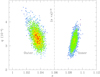 |
Fig. 2 Scatter plots of points in the MCMC chain on the (s, q) parameter plane. The colour scheme is configured to represent points with <1σ (red), <2σ (yellow), <3σ (green), <4σ (cyan), and <5σ (blue). The dotdashed vertical line in the left panel indicates the geometric mean of sin and sout. |
Best-fit lensing parameters.
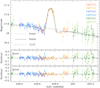 |
Fig. 3 Model curves of the inner and outer 2L1S solutions and their residuals in the region around the anomaly. |
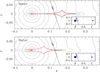 |
Fig. 4 Configurations of the inner and outer solutions. In each panel, the red figure depicts the caustic, and the arrowed line represents the source trajectory. The grey curves surrounding the caustic indicate the equi-magnification contours. The inset provides a zoomed-out view showing the positions of the lens components, denoted by blue dots. The dotted curve in the inset illustrates the Einstein ring. |
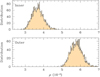 |
Fig. 5 Distributions of the normalised source radius for the inner and outer solutions. |
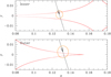 |
Fig. 6 Zoomed-in view of the caustic crossings for the inner and outer solutions. In each panel, the orange circle represents the source size scaled to the caustic size. |
4 Source star and angular Einstein radius
In this section we specify the source star of the event. Specifying the source is important not only for providing a comprehensive overview of the event but also for estimating the angular Einstein radius.
We specified the source star of the event using the methodology outlined in Yoo et al. (2004). First, we estimated the instrumental source magnitudes in the I and V passbands by linearly regressing the datasets, processed with the pyDIA photometry code (Albrow 2017), against the model light curve. Next, we placed the source in the colour-magnitude diagram (CMD) of stars near the source, constructed using the same pyDIA code. Finally, we calibrated the I- and V-band source magnitudes using the centroid of the red giant clump (RGC) in the CMD. The RGC centroid can be used for calibration because its (V − I) colour and I-band magnitude are known from previous studies conducted by Bensby et al. (2013) and Nataf et al. (2013).
Figure 7 shows the location of the source in the instrumental CMD of stars lying near the source. The measured instrumental colour and magnitude of the source are
![Mathematical equation: $\[(V-I, I)_\text{S}=(1.811 \pm 0.038,20.285 \pm 0.006).\]$](/articles/aa/full_html/2024/12/aa51620-24/aa51620-24-eq4.png) (3)
(3)
By measuring the offset, Δ(V − I, I) = (V − I, I)S − (V − I, I)RGC, between the source and RGC centroid, lying at (V − I, I)RGC = (1.987, 15.506), the de-reddened source colour and magnitude are estimated as
![Mathematical equation: $\[\begin{aligned}(V-I, I)_{\mathrm{S}, 0} & =(V-I, I)_{\mathrm{RGC}, 0}+\Delta(V-I, I) \\& =(0.884 \pm 0.055,19.118 \pm 0.021).\end{aligned}\]$](/articles/aa/full_html/2024/12/aa51620-24/aa51620-24-eq5.png) (4)
(4)
Here (V − I, I)RGC,0 = (1.060, 14.339) represent the de-reddened colour and magnitude of the RGC centroid. The estimated colour and magnitude indicate that the source is an early K-type main-sequence star. In the CMD, we also mark the location of the blend with a green dot. It is important to note that the instrumental colour and magnitudes are not precisely scaled, as the calculation of (V − I, I)S,0 relies only on the offset Δ(V − I, I), not on the absolute calibration of (V − I, I) and (V − I, I)RGC.
Based on the measured source colour and magnitude, we then estimated the angular radius of the source. For this, we first converted V − I colour into V − K colour using the Bessell & Brett (1988) colour-colour relation and then interpolated the angular source radius from the Kervella et al. (2004) relation between V − K and θ*. This yields the angular source radius of
![Mathematical equation: $\[\theta_{*}=(0.573 \pm 0.051) ~\mu\mathrm{as}.\]$](/articles/aa/full_html/2024/12/aa51620-24/aa51620-24-eq6.png) (5)
(5)
With the estimated source radius, the angular radius of the Einstein ring was estimated using the relation in Eq. (2) as
![Mathematical equation: $\[\theta_{\mathrm{E}}= \begin{cases}(0.166 \pm 0.021) ~\mathrm{mas},\quad\text {(inner solution), } \\ (0.100 \pm 0.010) \text { mas, }\quad\text {(outer solution). }\end{cases}\]$](/articles/aa/full_html/2024/12/aa51620-24/aa51620-24-eq7.png) (6)
(6)
It is important to note that the inner and outer solutions yield different values of the normalised source radius, which in turn result in different values of angular Einstein radius. With the determined value of θE together with the event timescale, estimated from the light curve modelling, the relative proper motion between the lens and source is determined as
![Mathematical equation: $\[\mu=\frac{\theta_{\mathrm{E}}}{t_{\mathrm{E}}}= \begin{cases}(6.59 \pm 0.82) ~\mathrm{mas} / \mathrm{yr},\quad\text { (inner solution), } \\ (4.01 \pm 0.42) ~\mathrm{mas} / \mathrm{yr},\quad\text { (outer solution). }\end{cases}\]$](/articles/aa/full_html/2024/12/aa51620-24/aa51620-24-eq8.png) (7)
(7)
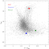 |
Fig. 7 Locations of the source and the centroid of the RGC in the instrumental CMD of stars in the vicinity of the source. Also marked is the location of the blend. |
5 Physical lens parameters
The mass (M) and distance (DL) of a microlens are constrained by measuring three lensing observables: tE, θE, and πE. Here the last observable πE denotes the microlens parallax. These observables are related to M and DL by the relations
![Mathematical equation: $\[t_{\mathrm{E}}=\frac{\theta_{\mathrm{E}}}{\mu}; \quad \theta_{\mathrm{E}}=\sqrt{\kappa M \pi_{\mathrm{rel}}}; \quad\quad \pi_{\mathrm{E}}=\left(\frac{\pi_{\mathrm{rel}}}{\theta_{\mathrm{E}}}\right)\left(\frac{\boldsymbol{\mu}}{\mu}\right),\]$](/articles/aa/full_html/2024/12/aa51620-24/aa51620-24-eq9.png) (8)
(8)
where κ = 4G/(c2AU), πrel = πL − πS = AU(1/DL −1/DS) is the relative lens-source parallax, DS represents the distance to the source, and μ denotes the vector of the relative lens-source proper motion (Gould 2000). For KMT-2024-BLG-1044, the event timescale and the angular Einstein radius were securely measured, but the microlens parallax could not be determined due to the combination of relatively large photometric uncertainties in the data and the short duration of the event. Consequently, we estimated the physical parameters of the lens through Bayesian analysis, using priors on the mass, location, and motion of lens objects within the Galaxy, and incorporating constraints from the measured observables.
In the Bayesian analysis, we first generated a large number of artificial events through a Monte Carlo simulation. In this simulation, the lens mass was derived from a mass-function model, while the distances to the lens and source, as well as the transverse lens-source speed (v⊥), were derived from a Galaxy model. We used the mass function model from Jung et al. (2022) and the Galaxy model from Jung et al. (2021). In the Galaxy model, the bulge density profile is represented by a triaxial distribution, while the disc matter density is described by a double-exponential distribution. For the stellar and BD mass functions, the initial mass function from Chabrier (2003) was applied to the bulge lens population, whereas the present-day mass function from the same source was used for the disc lens population. With the assigned physical parameters (Mi, DL,i, DS,i, v⊥,i) for each artificial event, we computed the corresponding lensing observables using the relations tE,i = DL,i θE,i/v⊥,i, θE,i = (κMi πrel,i)1/2, and πrel,i = AU(1/DL,i − 1/DS,i). In the second step, we constructed posterior distributions of the lens mass and distance by imposing a weight to the event of
![Mathematical equation: $\[w_{i}=\exp \left(\frac{\chi_{i}^{2}}{2}\right); \qquad \chi_{i}^{2}=\frac{\left(t_{\mathrm{E}, i}-t_{\mathrm{E}}\right)^{2}}{\sigma^{2}(t_{\mathrm{E}})}+\frac{\left(\theta_{\mathrm{E}, i}-\theta_{\mathrm{E}}\right)^{2}}{\sigma^{2}(\theta_{\mathrm{E}})}.\]$](/articles/aa/full_html/2024/12/aa51620-24/aa51620-24-eq10.png) (9)
(9)
Here (tE, θE) represent the measured values of the lensing observables, and [σ(tE), σ(θE)] are their measurement uncertainties. In the Bayesian analysis, we imposed an additional constraint, that the lens flux be less than the blended flux. However, this constraint had little effect on the posteriors because the estimated lens mass is very low.
In Figs. 8 and 9 we present the posterior distributions of the host mass and distance to the planetary system KMT-2024-BLG-1044L, respectively. We present two sets of distributions derived from separate analyses based on the inner and outer solutions, as these solutions result in substantially different values of θE. The estimated masses of the host and planet are
![Mathematical equation: $\[M_{\mathrm{h}}= \begin{cases}0.131_{-0.064}^{+0.146} ~M_{\odot},\quad\text { (inner solution), } \\ 0.069_{-0.036}^{+0.080} ~M_{\odot},\quad\text { (outer solution), }\end{cases}\]$](/articles/aa/full_html/2024/12/aa51620-24/aa51620-24-eq11.png) (10)
(10)
and
![Mathematical equation: $\[M_{\mathrm{p}}= \begin{cases}13.68_{-6.71}^{+15.23} ~M_{\mathrm{E}},\quad\text { (inner solution), } \\ 7.75_{-4.04}^{+12.03} M_{\mathrm{E}},\qquad\text { (outer solution), }\end{cases}\]$](/articles/aa/full_html/2024/12/aa51620-24/aa51620-24-eq12.png) (11)
(11)
respectively. Here we set the lower and upper limits of the physical parameters as the 16th and 84th percentiles of the Bayesian posteriors. The estimated physical parameters suggest that the planetary system consists of a host near the boundary between a star and a BD, with a planet possessing a mass smaller than that of Uranus. The estimated distance to the planetary system is
![Mathematical equation: $\[D_{\mathrm{L}}= \begin{cases}6.71_{-1.04}^{+0.99} ~\mathrm{kpc},\quad\text { (inner solution), } \\ 7.14_{-0.96}^{+0.95} ~\mathrm{kpc},\quad\text { (outer solution). }\end{cases}\]$](/articles/aa/full_html/2024/12/aa51620-24/aa51620-24-eq13.png) (12)
(12)
For the inner solution, the relative probabilities suggest a 25% chance of the lens lying in the disc and a 75% chance in the bulge. For the outer solution, these probabilities indicate a 17% chance in the disc versus 83% in the bulge. These probabilities indicate that the lens is more likely to be located in the bulge. The contributions from the disc and bulge lens populations were determined by summing the event rates of individual simulated microlensing events produced by lenses from each population.
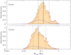 |
Fig. 8 Bayesian posteriors for the host mass of the planetary system KMT-2024-BLG-1044L. The distributions shown in the upper and lower panels are based on the inner and outer solutions, respectively. In each panel, the vertical solid line indicates the median value of the distribution, while the two dotted vertical lines denote the 1σ range. The distributions, depicted in blue and red, represent the contributions from the disc and bulge lens populations, respectively. The black curve represents the sum of these two contributions. |
6 Summary and discussion
We analysed microlensing data to understand the nature of the very short-term anomaly that appeared near the peak of the short-timescale microlensing event KMT-2024-BLG-1044. Detailed modelling of the light curve confirmed the planetary origin of the anomaly and revealed two possible solutions, due an to inner–outer degeneracy. The measured planet-to-host mass ratio is 3.1 × 10⁴ according to the inner solution and 3.4 × 10⁴ according to the outer solution. Using Bayesian analysis, constrained by both the short event timescale and the small angular Einstein radius, we have determined that the lens system is a planetary system. The mass estimates derived from this analysis suggest two possible interpretations for the nature of the host. According to the inner solution, the host star is likely a low-mass stellar object. However, the outer solution suggests that the host is a BD, with its mass falling into the substellar range. Resolving this degeneracy between the two possibilities presents significant challenges, primarily due to the limitations of the photometric data combined with the absence of spectroscopic data.
Moreover, the difficulty is compounded by the current lack of comprehensive knowledge regarding planet formation mechanisms in such systems, particularly for planets orbiting very low-mass stars and BDs. Matsuo et al. (2007) pointed out that additional information, such as the metallicity of the host star, could provide valuable constraints on the formation mechanism. Specifically, the two dominant models for planet formation, the core accretion model and the disc instability model, could be better differentiated with this kind of supplementary data. In the case of the KMT-2024-BLG-1044L system, however, it remains difficult to draw a definitive conclusion about the planet formation mechanism. This is because, while we have estimates for the masses of both the planet and its host, there is a lack of the critical additional information – such as host star metallicity – that would enable us to favour one formation mechanism over the other. Consequently, our current understanding of the system is limited, and further data would be required to make a more robust determination.
The discovery of the planetary system KMT-2024-BLG-1044L underscores the crucial role played by the microlensing technique in detecting planets that orbit substellar BDs or very low-mass stars. This is illustrated in Fig. 10, which depicts the distribution of extrasolar planets detected using the three major methods: transit, radial velocity, and microlensing. The data for the planets in the plot – 1149 transit planets, 195 radial velocity planets, and 221 microlensing planets with measured masses – were sourced from the NASA Exoplanet Archive. Within this dataset, there are 15 planetary systems for which the host has a substellar mass, defined as Mh ≲ 0.8 M⊙, or lying around the star-BD boundary. To investigate the common characteristics of BD-host planets, we present Table 3, which lists the planet and host masses, planet-to-host mass ratios, and lensing observables (tE, θE, and πE) for these planetary systems. For events with multiple degenerate solutions, we list the values of Mp and Mh that correspond to the individual solutions. Upon inspecting the lensing observables, we see that these planets can be broadly divided into two groups depending on how the BD nature of the host is identified. The first group, which includes MOA-2007-BLG-192, OGLE-2012-BLG-0358, and OGLE-2016-BLG-1195, was identified through the measurement of the large microlens parallax. The second group, which includes OGLE-2015-BLG-1771, KMT-2016-BLG-1820, KMT-2016-BLG-2142, KMT-2016-BLG-2605, OGLE-2017-BLG-1522, KMT-2018-BLG-0748, OGLE-2018-BLG-0677, KMT-2021-BLG-0371, KMT-2021-BLG-1554, and KMT-2024-BLG-1044, was identified primarily through the combination of short event timescales and the small angular radii of the Einstein rings. Notably, the discovery of all these planets has been made feasible through the unique capabilities of the microlensing method, particularly in detecting dark or faint celestial bodies. This highlights the method’s effectiveness in revealing planetary systems that might otherwise be challenging to detect using other observational methods.
Candidate microlensing planetary systems with BD hosts.
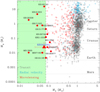 |
Fig. 10 Distribution of extrasolar planets detected using the three major methods – transit, radial velocity, and microlensing – in the plane of the host and planet masses. The green shade indicates the region where the host has a substellar mass. Red-filled dots represent planetary systems with masses near or below the star-brown dwarf mass threshold. The position of KMT-2024-BLG-1044L is marked with a triangle. |
Acknowledgements
J.C.Y. and I.-G.S. acknowledge support from U.S. NSF Grant No. AST-2108414. Y.S. acknowledges support from BSF Grant No. 2020740. This research has made use of the KMTNet system operated by the Korea Astronomy and Space Science Institute (KASI) at three host sites of CTIO in Chile, SAAO in South Africa, and SSO in Australia. Data transfer from the host site to KASI was supported by the Korea Research Environment Open NETwork (KREONET). This research was supported by KASI under the R&D program (Project No. 2024-1-832-01) supervised by the Ministry of Science and ICT. W.Z. and H.Y. acknowledge support by the National Natural Science Foundation of China (Grant No. 12133005). W.Z. acknowledges the support from the Harvard-Smithsonian Center for Astrophysics through the CfA Fellowship.
References
- Albrow, M. 2017, https://doi.org/10.5281/zenodo.268049 [Google Scholar]
- Albrow, M., Beaulieu, J.-P., Birch, P., et al. 1998, ApJ, 509, 687 [NASA ADS] [CrossRef] [Google Scholar]
- Albrow, M., Horne, K., Bramich, D. M., et al. 2009, MNRAS, 397, 2099 [Google Scholar]
- Alcock, C., Akerlof, C. W., Allsman, R. A., et al. 1993, Nature, 365, 621 [NASA ADS] [CrossRef] [Google Scholar]
- Alcock, C., Allen, W. H., Allsman, R. A., et al. 1997, ApJ, 491, 436 [Google Scholar]
- Bennett, D. P., Bond, I. A., Udalski, A., et al. 2008, ApJ, 684, 663 [Google Scholar]
- Bennett, D. P., Batista, V., Bond, I. A., et al. 2014, ApJ, 785, 155 [Google Scholar]
- Bensby, T., Yee, J. C., Feltzing, S., et al. 2013, A&A, 549, A147 [NASA ADS] [CrossRef] [EDP Sciences] [Google Scholar]
- Bessell, M. S., & Brett, J. M. 1988, PASP, 100, 1134 [Google Scholar]
- Bond, I. A., Abe, F., Dodd, R. J., et al. 2001, MNRAS, 327, 868 [Google Scholar]
- Bond, I. A., Udalski, A., Jaroszyński, M., et al. 2004, ApJ, 606, L155 [NASA ADS] [CrossRef] [Google Scholar]
- Chabrier, G. 2003, ApJ, 586, L133 [NASA ADS] [CrossRef] [Google Scholar]
- Dong, S., DePoy, D. L., Gaudi, B. S., et al. 2006, ApJ, 642, 842 [NASA ADS] [CrossRef] [Google Scholar]
- Doran, M., & Mueller, C. M. 2004, J. Cosmol. Astropart. Phys., 09, 003 [CrossRef] [Google Scholar]
- Gaudi, B. S. 1998, ApJ, 506, 533 [Google Scholar]
- Gaudi, B. S. 2012, ARA&A, 50, 411 [Google Scholar]
- Gaudi, B. S., & Gould, A. 1997, ApJ, 486, 85 [Google Scholar]
- Gould, A. 2000, ApJ, 542, 785 [NASA ADS] [CrossRef] [Google Scholar]
- Gould, A., & Loeb, A. 1992, ApJ, 396, 104 [Google Scholar]
- Gould, A., Udalski, A., An, D., et al. 2006, ApJ, 644, L37 [Google Scholar]
- Gould, A., Han, C., Zang, W., et al. 2022, A&A, 664, A13 [NASA ADS] [CrossRef] [EDP Sciences] [Google Scholar]
- Han, C., Jung, Y. K., & Udalski, A. 2013, ApJ, 778, 38 [NASA ADS] [CrossRef] [Google Scholar]
- Han, C., Shin, I.-G., Jung, Y. K., et al. 2020, A&A, 641, A105 [NASA ADS] [CrossRef] [EDP Sciences] [Google Scholar]
- Han, C., Kim, D., Gould, A., et al. 2022, A&A, 664, A33 [NASA ADS] [CrossRef] [EDP Sciences] [Google Scholar]
- Herrera-Martín, A., Albrow, M. D., Udalski, A., et al. 2020, AJ, 159, 256 [Google Scholar]
- Hwang, K.-H., Zang, W., Gould, A., et al. 2022, AJ, 163, 43 [NASA ADS] [CrossRef] [Google Scholar]
- Jung, Y. K., Udalski, A., Gould, A., et al. 2018, AJ, 155, 219 [Google Scholar]
- Jung, Y. K., Han, C., Udalski, A., et al. 2021, AJ, 161, 293 [NASA ADS] [CrossRef] [Google Scholar]
- Jung, Y. K., Zang, W., Han, C., et al. 2022, AJ, 164, 262 [NASA ADS] [CrossRef] [Google Scholar]
- Jung, Y. K., Hwang, K.-H., Yang, H., et al. 2024, AJ, 168, 152 [NASA ADS] [CrossRef] [Google Scholar]
- Kervella, P., Thévenin, F., Di Folco, E., & Ségransan, D. 2004, A&A, 426, 29 [Google Scholar]
- Kim, S.-L., Lee, C.-U., Park, B.-G., et al. 2016, J. Korean Astron. Soc., 49, 37 [Google Scholar]
- Kim, D.-J., Kim, H.-W., & Hwang, K.-H. 2018, AJ, 155, 76 [NASA ADS] [CrossRef] [Google Scholar]
- Kim, H.-W., Hwang, K.-H., Gould, A., et al. 2021a, AJ, 162, 15 [NASA ADS] [CrossRef] [Google Scholar]
- Kim, Y. H., Chung, S.-J., Yee, J. C., et al. 2021b, AJ, 162, 17 [NASA ADS] [CrossRef] [Google Scholar]
- Koshimoto, N., Sumi, T., Bennett, D. P., et al. 2023, AJ, 166, 107 [NASA ADS] [CrossRef] [Google Scholar]
- Mao, S., & Paczyński, B. 1991, ApJ, 374, L37 [Google Scholar]
- Matsuo, T., Shibai, H., Ootsubo, T., & Tamura, M. 2007, ApJ, 662, 1282 [NASA ADS] [CrossRef] [Google Scholar]
- Miyazaki, S., Sumi, T., Bennett, D. P., et al. 2018, AJ, 156, 136 [Google Scholar]
- Mróz, P., Ryu, Y.-H., Skowron, J., et al. 2018, AJ, 155, 121 [Google Scholar]
- Mróz, P., Udalski, A., Bennett, D. P., et al. 2019, A&A, 622, A201 [NASA ADS] [CrossRef] [EDP Sciences] [Google Scholar]
- Mróz, P., Poleski, R., Gould, A., et al. 2020a, ApJ, 903, L11 [Google Scholar]
- Mróz, P., Poleski, R., Han, C., et al. 2020b, AJ, 159, 262 [CrossRef] [Google Scholar]
- Nataf, D. M., Gould, A., Fouqué, P., et al. 2013, ApJ, 769, 88 [Google Scholar]
- Ryu, Y.-H., Mróz, P., Gould, A., et al. 2021a, AJ, 161, 126 [NASA ADS] [CrossRef] [Google Scholar]
- Ryu, Y.-H., Hwang, K.-H., Gould, A., et al. 2021b, AJ, 162, 96 [NASA ADS] [CrossRef] [Google Scholar]
- Shvartzvald, Y., Yee, J. C., Novati, S. C., et al. 2017, ApJ, 840, L3 [NASA ADS] [CrossRef] [Google Scholar]
- Sumi, T., Udalski, A., Bennett, D. P., et al. 2016, ApJ, 825, 112 [Google Scholar]
- Suzuki, D., Bennett, D. P., Sumi, T., et al. 2016, ApJ, 833, 145 [Google Scholar]
- Tsapras, Y., Horne, K., Kane, S., & Carson, R. 2003, MNRAS, 343, 1131 [NASA ADS] [CrossRef] [Google Scholar]
- Udalski, A., Szymanski, M., Kałużny, J., et al. 1994, Acta Astron., 44, 1 [NASA ADS] [Google Scholar]
- Yang, H., Yee, J. C., Hwang, K.-H., et al. 2024, MNRAS, 528, 11 [NASA ADS] [CrossRef] [Google Scholar]
- Yee, J. C., Shvartzvald, Y., Gal-Yam, A., et al. 2012, ApJ, 755, 102 [Google Scholar]
- Yee, J. C., Zang, W., Udalski, A., et al. 2021, AJ, 162, 180 [NASA ADS] [CrossRef] [Google Scholar]
- Yoo, J., DePoy, D. L., Gal-Yam, A., et al. 2004, ApJ, 603, 139 [Google Scholar]
- Zhang, K., & Gaudi, B. S. 2022, ApJ, 936, L22 [NASA ADS] [CrossRef] [Google Scholar]
- Zhang, X., Zang, W., Udalski, A., et al. 2020, AJ, 159, 116 [Google Scholar]
- Zhang, K., Gaudi, B. S., & Bloom, J. S. 2022, Nat. Astron., 6, 782 [NASA ADS] [CrossRef] [Google Scholar]
Currently, nine free-floating planet candidates have been reported (Mróz et al. 2018, 2019, 2020a,b; Kim et al. 2021a; Ryu et al. 2021a; Koshimoto et al. 2023; Jung et al. 2024).
All Tables
All Figures
|
Fig. 1 Light curve of the lensing event KMT-2024-BLG-1044. Lower panel: full view of the light curve. Upper panel: zoomed-in view of the peak region around the anomaly. The solid curve drawn over the data points is a single-lens single-source model obtained by fitting the data excluding those around the anomaly. The colours of the data points correspond to those of the datasets marked in the legend. |
| In the text | |
|
Fig. 2 Scatter plots of points in the MCMC chain on the (s, q) parameter plane. The colour scheme is configured to represent points with <1σ (red), <2σ (yellow), <3σ (green), <4σ (cyan), and <5σ (blue). The dotdashed vertical line in the left panel indicates the geometric mean of sin and sout. |
| In the text | |
|
Fig. 3 Model curves of the inner and outer 2L1S solutions and their residuals in the region around the anomaly. |
| In the text | |
|
Fig. 4 Configurations of the inner and outer solutions. In each panel, the red figure depicts the caustic, and the arrowed line represents the source trajectory. The grey curves surrounding the caustic indicate the equi-magnification contours. The inset provides a zoomed-out view showing the positions of the lens components, denoted by blue dots. The dotted curve in the inset illustrates the Einstein ring. |
| In the text | |
|
Fig. 5 Distributions of the normalised source radius for the inner and outer solutions. |
| In the text | |
|
Fig. 6 Zoomed-in view of the caustic crossings for the inner and outer solutions. In each panel, the orange circle represents the source size scaled to the caustic size. |
| In the text | |
|
Fig. 7 Locations of the source and the centroid of the RGC in the instrumental CMD of stars in the vicinity of the source. Also marked is the location of the blend. |
| In the text | |
|
Fig. 8 Bayesian posteriors for the host mass of the planetary system KMT-2024-BLG-1044L. The distributions shown in the upper and lower panels are based on the inner and outer solutions, respectively. In each panel, the vertical solid line indicates the median value of the distribution, while the two dotted vertical lines denote the 1σ range. The distributions, depicted in blue and red, represent the contributions from the disc and bulge lens populations, respectively. The black curve represents the sum of these two contributions. |
| In the text | |
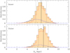 |
Fig. 9 Bayesian posteriors for the distance to the lens. The notations are same in Fig. 8. |
| In the text | |
|
Fig. 10 Distribution of extrasolar planets detected using the three major methods – transit, radial velocity, and microlensing – in the plane of the host and planet masses. The green shade indicates the region where the host has a substellar mass. Red-filled dots represent planetary systems with masses near or below the star-brown dwarf mass threshold. The position of KMT-2024-BLG-1044L is marked with a triangle. |
| In the text | |
Current usage metrics show cumulative count of Article Views (full-text article views including HTML views, PDF and ePub downloads, according to the available data) and Abstracts Views on Vision4Press platform.
Data correspond to usage on the plateform after 2015. The current usage metrics is available 48-96 hours after online publication and is updated daily on week days.
Initial download of the metrics may take a while.