| Issue |
A&A
Volume 683, March 2024
|
|
|---|---|---|
| Article Number | A187 | |
| Number of page(s) | 12 | |
| Section | Planets and planetary systems | |
| DOI | https://doi.org/10.1051/0004-6361/202348245 | |
| Published online | 19 March 2024 | |
KMT-2023-BLG-0416, KMT-2023-BLG-1454, KMT-2023-BLG-1642: Microlensing planets identified from partially covered signals
1
Department of Physics, Chungbuk National University,
Cheongju
28644,
Republic of Korea
e-mail: cheongho@astroph.chungbuk.ac.kr
2
Astronomical Observatory, University of Warsaw,
Al. Ujazdowskie 4,
00-478
Warszawa,
Poland
3
Korea Astronomy and Space Science Institute,
Daejon
34055,
Republic of Korea
4
Department of Astronomy and Tsinghua Centre for Astrophysics, Tsinghua University,
Beijing
100084,
PR China
5
University of Canterbury, Department of Physics and Astronomy,
Private Bag 4800,
Christchurch
8020,
New Zealand
6
Korea University of Science and Technology,
217 Gajeong-ro, Yuseong-gu,
Daejeon
34113,
Republic of Korea
7
Max Planck Institute for Astronomy,
Königstuhl 17,
69117
Heidelberg,
Germany
8
Department of Astronomy, The Ohio State University,
140 W. 18th Ave.,
Columbus,
OH
43210,
USA
9
Department of Particle Physics and Astrophysics, Weizmann Institute of Science,
Rehovot
76100,
Israel
10
Center for Astrophysics | Harvard & Smithsonian
60 Garden St.,
Cambridge,
MA
02138,
USA
11
School of Space Research, Kyung Hee University,
Yongin,
Kyeonggi
17104,
Republic of Korea
12
Department of Physics, University of Warwick,
Gibbet Hill Road,
Coventry,
CV4 7AL,
UK
Received:
12
October
2023
Accepted:
10
January
2024
Aims. We investigate the 2023 season data from high-cadence microlensing surveys with the aim of detecting partially covered shortterm signals and revealing their underlying astrophysical origins. Through this analysis, we ascertain that the signals observed in the lensing events KMT-2023-BLG-0416, KMT-2023-BLG-1454, and KMT-2023-BLG-1642 are of planetary origin.
Methods. Considering the potential degeneracy caused by the partial coverage of signals, we thoroughly investigate the lensing-parameter plane. In the case of KMT-2023-BLG-0416, we have identified two solution sets, one with a planet-to-host mass ratio of q ~ 10−2 and the other with q ~ 6 × 10⁻⁵, within each of which there are two local solutions emerging due to the inner-outer degeneracy. For KMT-2023-BLG-1454, we discern four local solutions featuring mass ratios of q ~ (1.7−4.3) × 10−3. When it comes to KMT-2023-BLG-1642, we identified two locals with q ~ (6 − 10) × 10−3 resulting from the inner-outer degeneracy.
Results. We estimate the physical lens parameters by conducting Bayesian analyses based on the event time scale and Einstein radius. For KMT-2023-BLG-0416L, the host mass is ~0.6 M⊙, and the planet mass is ~(6.1−6.7) MJ according to one set of solutions and ~0.04 MJ according to the other set of solutions. KMT-2023-BLG-1454Lb has a mass roughly half that of Jupiter, while KMT-2023-BLG-1646Lb has a mass in the range of between 1.1 to 1.3 times that of Jupiter, classifying them both as giant planets orbiting mid M-dwarf host stars with masses ranging from 0.13 to 0.17 solar masses.
Key words: gravitation / gravitational lensing: micro / planets and satellites: detection
© The Authors 2024
 Open Access article, published by EDP Sciences, under the terms of the Creative Commons Attribution License (https://creativecommons.org/licenses/by/4.0), which permits unrestricted use, distribution, and reproduction in any medium, provided the original work is properly cited.
This article is published in open access under the Subscribe to Open model. Subscribe to A&A to support open access publication.
1 Introduction
The microlensing signature of a planet, in general, manifests as a brief transient anomaly within the lensing light curve produced by the host of the planet (Mao & Paczyński 1991; Gould & Loeb 1992). Detecting such a brief signal posed a formidable challenge in the early stage of microlensing experiments, such as the Optical Gravitational Lensing Experiment (OGLE; Udalski et al. 1994) and Massive Astrophysical Compact Halo Object (MACHO; Alcock et al. 1995) experiments, in which lensing events were observed at approximately one-day intervals. In the 1990s and 2000s, the necessary observational frequency to detect planetary signals was achieved through the implementation of early warning systems, as exemplified by the pioneering work of Udalski et al. (1994) and Alcock et al. (1996). These systems were coupled with subsequent observations of alerted events, conducted by various follow-up teams, including Galactic Microlensing Alerts Network (GMAN; Alcock et al. 1997), Probing Lensing Anomalies NETwork (PLANET; Albrow et al. 1998), Microlensing Follow-Up Network (μFUN; Yoo et al. 2004b), and RoboNet (Tsapras 2003). For an in-depth exploration on the historical development of the observational strategies implemented during this era, we recommend referring to the comprehensive review of Gould et al. (2010).
In contemporary microlensing experiments, the essential high-frequency observations necessary for capturing short planetary signals are made possible through utilizing a network of globally dispersed telescopes which are equipped with very wide-field cameras. Regarding the Korea Microlensing Telescope Network (KMTNet; Kim et al. 2016) survey, the observational frequency in its primary fields is reduced to as little as 15 min, a time frame sufficiently brief to detect signals generated by a planet with a mass similar to that of Earth. With the capability to continuously monitor all lensing events and discern signals emerging from various segments of lensing light curves, contemporary lensing surveys are now detecting an estimated 30 planets on an annual basis (Gould 2022; Gould et al. 2022; Jung et al. 2022).
Although the current microlensing surveys have improved their observational cadence, there are still gaps in the coverage of a portion of planetary signals. Weather conditions at telescope sites are the primary factor responsible for the incomplete coverage of planetary signals. Planetary signals typically exhibit durations spanning several days for giant planets and several hours for terrestrial planets, and incomplete coverage of these signals occasionally occurs when adverse weather conditions at telescope sites across the global network hinder observations. The discontinuous coverage of planetary signals can also be attributed to another factor: the temporal gaps between observation times at different telescope sites. In practical terms, this means that some lensing events can be observable for only a portion of a night, resulting in a time lag between observations at one site and the subsequent observations at another site. The significance of this gap in observation times is particularly pronounced during the initial and concluding phases of the bulge season when the available observation periods are relatively short. Finally, planetary signals from events occurring in certain fields covered with relatively low cadences tend to be incomplete, particularly for events characterized by very brief anomalies in duration. It is crucial to scrutinize partially covered signals because planets associated with these signals might remain unreported without in-depth analyses. Neglecting such analyses could lead to inaccurate estimations of the detection efficiency, which is a fundamental element for establishing the demographics of planets detected through microlensing.
In this paper, we report the discoveries of three microlensing planets from the analyses of the lensing events KMT-2023-BLG-0416, KMT-2023-BLG-1454, and KMT-2023-BLG-1642, for which the planetary signals within the lensing light curves were only partially observed. The event analyses were carried out as a component of a project focused on exploring brief transient anomalies with limited data coverage, aiming to identify potential planetary candidates. The initial publication of planetary discoveries stemming from the analysis of data gathered during the 2021 and 2022 seasons of the KMTNet survey was documented in Han et al. (2023). The analyses presented in this work constitute the project’s second release of results, this time stemming from the investigation of data gathered during the 2023 season of the KMTNet survey.
2 Data and observations
The anomalies in the three microlensing events KMT-2023-BLG-0416, KMT-2023-BLG-1454, and KMT-2023-BLG-1642 were found through the examination of lensing events detected during the 2023 season by the KMTNet survey. This survey focuses on the monitoring of stars lying toward the Galactic bulge field in the quest for gravitational lensing events. To achieve continuous coverage of lensing events, the survey employs three identical telescopes positioned across the three continents in the Southern Hemisphere. The sites of the individual KMTNet telescopes are the Cerro Tololo Interamerican Observatory in Chile (KMTC), the South African Astronomical Observatory in South Africa (KMTS), and the Siding Spring Observatory in Australia (KMTA). Each of the KMTNet telescopes has a 1.6 m aperture and is equipped with a wide-field camera that delivers a field of view spanning 4 square degrees. The survey primarily employs the I band for image acquisition, with approximately ten percent of the images obtained in the V band, specifically for the purpose of source color measurement. The observation cadences vary depending on the events: 1.0 h for KMT-2023-BLG-0416, 0.25 h for KMT-2023-BLG-1454, and 2.5 h for KMT-2023-BLG-1642. Among the events, KMT-2023-BLG-0416 was additionally identified by the OGLE group. During its fourth phase, the OGLE survey is conducted with the use of the 1.3-meter telescope that lies at the Las Campanas Observatory in Chile. The OGLE telescope is equipped with a camera that provides a field of view encompassing 1.4 square degrees. In the analysis of KMT-2023-BLG-0416, we include the OGLE data.
The preliminary image reduction and source photometry were conducted using the data processing pipelines developed by Albrow et al. (2009) for the KMTNet survey and Udalski (2003) for the OGLE survey. For the use of optimal data in the analyses, the KMTNet data were reprocessed using the updated KMTNet pipeline, which was recently developed by Yang et al. (2024) and planned to be implemented from the 2024 season. To construct color-magnitude diagrams (CMDs) for stars lying near the source stars and to derive source magnitudes in the I and V passbands, supplementary photometry was carried out on the KMTC dataset using the pyDIA code developed by Albrow (2017). We re-calibrated the error bars associated with the photometry data obtained from the pipelines in accordance with the procedure outlined in Yee et al. (2012). In this procedure, the error bars are normalized by  , where σi represents the photometry error estimated from the pipeline. The values of k and σmin are chosen so that the χ2 value per degree of freedom (d.o.f.) for each dataset becomes unity and the cumulative sum of χ2 is approximately linear as a function of source magnification. The cumulative sum of χ2 is constructed by first sorting the data points of each dataset by magnification, calculating the value of
  contributed by each point, and then plotting
  as a function of N. Here N denotes the number of data points with magnification less than or equal to the magnification of point N. Figure 1 shows the cumulative sum of χ2 for the individual datasets of the three analyzed events.
This calibration was performed to ensure that the error bars are consistent with the scatter of data.
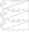 |
Fig. 1 Cumulative sum of χ2 for the individual datasets of the three analyzed events KMT-2023-BLG-0416, KMT-2023-BLG-1454, and KMT-2023-BLG-1642. The colors of the distributions match those of the datasets marked in the legend. |
3 Light curve analyses
It turns out that the anomalies in the light curves of the analyzed lensing events are very likely to be generated by planetary companions to the lenses. We start by offering an introductory overview of the fundamental physics of planetary lensing, which serves to introduce pertinent terminology, elucidate the modeling procedure, and clarify the parameters employed in the modeling process, before proceeding with in-depth event analyses.
A planet-induced anomaly arises when the source of a lensing event passes over or approaches close to the caustics induced by the planet. Caustics represent positions on the source plane where the lensing magnification of a point source becomes infinitely large. In the case of a lens composed of a single planet and its host, with a planet/host mass ratio less than order of 10−3, the lensing behavior is described by a binary-lens single-source (2L 1S) formalism with a very low mass ratio. Typically, a planet generates two distinct sets of caustics: one set, known as the central caustic, is situated in close proximity to the position of the planet host, while the other set, referred to as the planetary caustic, is located away from the host at a position approximately ~(1 − 1/s2)s1. Here s denotes the position vector of the planet from the host with its length normalized to the angular Einstein radius θE of the lens-system. From the perspective of the lens plane, planetary anomalies occur when the planet perturbs one of the two source images formed by the planet’s host. When the planet perturbs the brighter (major) image, the image is further magnified and the resulting anomaly exhibits a positive deviation. On the other hand, when the planet perturbs the fainter (minor) image, the image is often demagnified, which then results in a negative deviation (Gaudi & Gould 1997).
The number and shape of the planet-induced caustics vary depending on the projected separation and mass ratio between the planet and host. Planet-induced caustics are classified into three topologies: “close”, “wide”, and “resonant” (Erdl & Schneider 1993). A close planet induces a pair of planetary caustics positioned on the opposite side of the planet with respect to the primary, whereas a wide planet induces a single planetary caustic on the planet side. In the case of a resonant caustic, the planetary and central caustics merge together, resulting in a unified set of caustics. The detailed descriptions on the shapes and characteristics of the central and planetary caustics are extensively covered in the works of Chung et al. (2005) and Han (2006), respectively.
Assuming that the relative motion between the lens and source is rectilinear, the light curve of a planetary event can be described using seven parameters. The first set of three parameters (t0, u0, tE) characterizes the approach of the source to the lens, and the individual parameters denote the time of the closest approach, the lens-source separation at t0 (impact parameter, scaled to θE), and the event time scale. Another set of three parameters (s, q, α) characterize the binary lens, and the parameters denote the projected separation (normalized to θE), the mass ratio, and the angle between the source trajectory and the binary-lens axis (source trajectory angle), respectively. The last parameter ρ, which is defined as the ratio of the angular source radius θ* to θE, serves to describe the deformation of the lensing light curve by finite-source effects, which become prominent as the source approaches very near to the caustic or passes over it.
We analyze the events by modeling the light curves in search for the lensing solutions of the individual events. The term “lensing solution” refers to the collection of lensing parameters that most accurately describe the observed light curve. In the 2L 1S modeling, the searches for the parameters are done in two steps. In the first step, we seek the binary parameters s and q through a grid-based approach, employing multiple initial values of α. Subsequently, we determine the remaining parameters through a downhill method. In this downhill approach, we find the lensing parameters by minimizing χ2 using the Markov chain Monte Carlo (MCMC) technique, which incorporates a Gaussian sampler with an adaptable step size, as outlined in Doran & Mueller (2004). The initial step in this procedure results in a ∆χ2 map across the grid parameters, that is, (s, q). We identify local solutions that manifest on the (s, q) parameter plane. In the second step, we further refine the initially identified local solutions and determine a global solution by evaluating the goodness of fit across these local solutions. In the case of the lensing events examined in this study, the observed anomalies on the light curves are only partially observable, potentially leading to various forms of degeneracy when interpreting these anomalies. Consequently, it becomes crucial to investigate and consider these degenerate solutions in order to make accurate interpretations of the observed anomalies.
3.1 KMT-2023-BLG-0416
The source star of the lensing event KMT-2023-BLG-0416 lies at the equatorial coordinates (RA, Dec) = (17:45:17.77, −25:04:46.16), which correspond to the Galactic coordinates (l, b) = (3°.255, 2°.071). The I-band magnitude of the source before the lensing magnification, baseline magnitude, is Ibase = 20.41, and the extinction toward the field is AI = 3.02. The event was first found by the KMTNet group on 2023 April 17, which corresponds to the abridged heliocentric Julian date HJD′ ≡ HJD − 2460000 ~ 51. At the time of finding the event, the source was brighter than the baseline magnitude by ∆I ~ 1.86. The OGLE group independently detected the event 10 days after its initial discovery by KMTNet and labeled the event as OGLE-2023-BLG-0402. Hereafter we refer to the event using the event ID provided by the KMTNet group in accordance with the convention that adopts the event ID assigned by the initial discovery group.
The lensing light curve of KMT-2023-BLG-0416 constructed with the combined KMTNet and OGLE data is shown in Fig. 2. The lower panel provides an overview, while the upper panel offers a close-up view of the area indicated by the arrow in the lower panel. The curve drawn over the data points is the single-lens single-source (1L 1S) model obtained by fitting the data excluding those around the anomaly. From the detailed inspection of the light curve, we found that the light curve exhibited a partially covered short-term anomaly in the region around HJD′ ~ 54.9. The ascending segment of the anomaly was captured by the data obtained through observations carried out with the Chilean telescopes, specifically KMTC and OGLE data. However, the subsequent portion of the anomaly remained unobserved due to cloud cover at the Australian observation site. Although only a small portion of the anomaly was covered, the signal is very likely to be real because both the KMTC and OGLE observations verified the ascending segment of the anomaly. In addition to the ascending segment, the anomaly displays minor negative deviations preceding the rise, and this suggests that the rising anomaly pattern resulted from the source crossing over a caustic induced by a lens companion.
Considering the caustic-related feature of the anomaly, we conducted a 2L 1S modeling of the event. For the thorough exploration of all potential solutions capable of explaining the observed anomaly, we conducted an extensive grid search for the binary parameters s and q. Figure 3 shows the ∆χ2 map on the (log s, log q) parameter plane constructed from the grid search. We identified two sets of local solutions, in which one set has a mass ratio between the lens components of log q ~ −2.0 (local A), and the other set has a mass ratio of log q ~ −4.1 (local B). For each set, there exist a pair of solutions, designated as “inner” and “outer” solutions, and thus we identified four local solutions in total: “Ain”, “Aout”, “Bin”, and “Bout”. Below, we explain the choice of the notations “inner” and “outer” used to designate the solutions. In Fig. 3, we mark the individual local solutions in the ∆χ2 map.
In Table 1, we list the lensing parameters of the individual local solutions together with χ2 values of the fit and degree of freedom. For each solution, the lensing parameters are refined by permitting them to vary from the initial values found from the first-round of modeling using the grid approach. The binary parameters of the solutions Ain and Aout are (s, q)in ~ (1.37, 9.7 × 10⁻³) and (s, q)out ~ (0.77, 10.0 × 10⁻³), respectively, and those of the solutions Bin and Bout are (s, q)in ~ (1.054, 6.6 × 10⁻⁵) and (s, q)out ~ (0.997, 6.2 × 10⁻⁵), respectively. Across all solutions, the mass ratios between the lens components remain below 10−2, affirming that the companion to the lens is a planetary-mass object. The local solutions Bin and Bout are preferred over their counterparts Ain and Aout by ∆χ2 = 12.9 and 6.1, respectively.
In Fig. 4, we present the model curves of the Aout (dotted curve) and Bout (solid curve) solutions in the region around the anomaly. We note that the model curves of the Ain and Bin solutions are similar to those of the corresponding outer solutions Aout and Bout. Although the solution B provides a slightly better fit to the anomaly than the solution A, both solutions approximately describe the anomaly feature. However, their model curves diverge significantly after the last data point of the anomaly within the time range 54.9 ≲ HJD′ ≲ 55.8. This discrepancy suggests that the apparent degeneracy between solutions A and B is likely due to the incomplete coverage of the anomaly rather than a fundamental physical degeneracy.
Figure 5 shows the lens-system configurations of the four degenerate solutions. From the comparison of the configurations, we find that the similarities between the model curves of the pair of the Ain–Aout solutions and the pair of the Bin–Bout solutions are caused by the “inner-outer” degeneracy. This degeneracy was originally proposed by Gaudi & Gould (1997) to point out the similarity between the planetary signals produced by the source passage through the near (inner) and far (outer) sides of the planetary caustic. Later Yee et al. (2021) found that the degeneracy can be extended to planetary signals induced by central and resonant caustics. Hwang et al. (2022) and Gould (2022) derived an analytic relation between the binary separations of the inner and outer solutions, sin and sout. The relation is expressed as
 (1)
(1)
where  , τanom = (tanom − tanom denotes the time of the planet-induced anomaly, and the “+” and “−” signs apply to the anomalies exhibiting positive and negative deviations, resulting from the major and minor image perturbations, respectively. With the values of (t0, u0, tE, tanom) ~ (54.2, 0.023, 28.0, 55.4) for the pair of the Ain−Aout solutions, we find that
  , which matches well the geometric mean of the binary separations of
  . For the pair of the Bin−Bout solutions with (t0, u0, tE, tanom) ~ (53.9, 0.033, 24, 54.9), we find that
  , which also matches very well the geometric mean
  . The fact that the binary separations of the pair of solutions with similar model curves well follow the relation in Eq. (1) indicates that the model curves are subject to the inner–outer degeneracy. In Fig. 2, we mark the geometric mean of sin and sout for the B solutions as a vertical dot-dashed line.
Because it is known that a short-term positive deviation can also be produced by a faint companion to the source (Gaudi 1998), we additionally checked for a possible binary-source origin of the anomaly. The model curve of the single-lens binary-source (1L2S) solution and the residual from the model are presented in Fig. 4. We find that the 1L2S solution yields a model that is worse than the 2L1S model by ∆χ2 = 24.6, which is most pronounced in the region just before the major positive anomaly. As a result, we rule out the binary-source explanation for the anomaly.
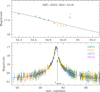 |
Fig. 2 Lensing light curve of KMT-2023-BLG-0416. The lower panel presents the overall perspective, while the upper panel provides a close-up view of the anomaly region. The arrow in the lower panel indicates the time of the anomaly. The curve drawn over the data points is a 1L 1S model obtained by fitting the light curve with the exclusion of the data around the anomaly. |
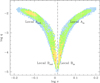 |
Fig. 3 ∆χ2 map on the plane of the planet parameters (log s, log q) of the lensing event KMT-2023-BLG-0416. The color scheme represents points with ∆χ2 < 12n (red), < 22n (yellow), < 32n (green), and < 42n (cyan), where n = 2. The labels marked by Ain, Aout, Bin, and Bout represent positions of the four local solutions. The vertical dot-dashed line indicates the geometric mean between the binary separations of the Bin and Bout solutions. |
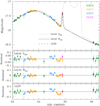 |
Fig. 4 Model curves of the local solutions Aout and Bout for KMT-2023-BLG-0416. The lower panels show the residuals from the two local planetary solutions and the single-lens binary-source (1L2S) solution. |
Solutions of KMT-2023-BLG-0416.
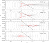 |
Fig. 5 Lens-system configurations of the four local solutions of KMT-2023-BLG-0416. In each panel, the red cuspy figure represents the caustic, the arrowed line is the source trajectory, and the grey curves surrounding the caustic represent the equi-magnification contours. |
3.2 KMT-2023-BLG-1454
The lensing event KMT-2023-BLG-1454 occurred on a star lying at the equatorial and Galactic coordinates of (RA, Dec) = (17:50:28.82, −29:37:21.90) and (l, b) = (−0°.040, −1°.262), respectively. The source has a baseline magnitude Ibase = 18.23, and the extinction toward the field is AI = 3.09. The event was found by the KMTNet group on 2023 June 29 (HJD′ = 124). One day after the event detection, the event reached its peak with a magnification of Apeak ~ 34. The duration of the event is relatively short, and the source flux returned to its baseline about a week after reaching the peak.
In Fig. 6, we present the light curve of KMT-2023-BLG-1454. The source of the event lies in the overlapping region of the two KMTNet prime fields BLG02 and BLG42, for which observations were conducted at a cadence of 0.5 h for each field and 0.25 h for the overlapping area of the two fields. In the analysis, we do not include the KMTA dataset not only because the peak region, near which an anomaly occurred, was not covered by these data, but also because the uncertainties in these data are large. From inspection of the light curve, we found that an anomaly occurred near the peak, as shown in the upper panel of Fig. 6. The anomaly displays two separate features, in which the feature centered at HJD′ ~ 125.7 exhibits both rising and falling deviations with respect to a 1L1S model, and the other feature centered at HJD′ ~ 126.5 shows only a falling deviation. The structure of the anomaly could not be fully delineated due to the absence of the KMTA dataset, which could have spanned the gap between the KMTC and KMTS data if it were not for the cloud cover at the Australian site. While a companion to a source can produced anomalies with only a single anomaly feature, a companion to a lens can produced anomalies with multiple features. Therefore, the anomaly is likely to be produced by a lens companion.
Considering the characteristics of the anomaly, we conducted a 2L 1S modeling of the lensing light curve. The ∆χ2 map on the (log s, log q) parameter plane constructed from the grid search is shown in Fig. 7. The map shows four distinct local solutions, with binary parameters (log s, log q) ~ (−0.045, −2.45) (local A), ~ (−0.01, −2.78) (local B), ~ (0.007, −2.50) (local C), and ~ (0.05, −2.36) (local D). Although the mass ratios of the local solutions exhibit slight differences, they consistently represent planet-to-star mass ratios across all solutions. In Table 2, we list the refined lensing parameters of the individual local solutions together with the χ2 values of the fits. It is found that the local solution A is preferred over the other solutions by ∆χ2 ≥ 9.9. The time scale of the event, tE ~ 6.4 day, is short. To be discussed below, both anomaly features centered at HJD′ ~ 125.7 and ~ 126.5 were produced by the source crossings over a caustic, and thus the normalized source radius, ρ ~ 21.5 × 10⁻³, is measured.
In Fig. 8, we present the model curves of the four local solutions together with the residuals from the models in the region around the anomaly. Figure 9 shows the configurations of the lens systems corresponding to the individual local solutions. For all solutions, the caustic displays a resonant form, in which the planetary caustics are connected with the central caustics. It is found that the solutions A and D are the pair of solutions arising from the inner-outer degeneracy. According to the configurations, the source passed the inner region between the central and planetary caustic in the case of the A solution (inner solution), while the source passed the outer region of the planetary caustic in the case of the D solution (outer solution). With the parameters (t0, u0, tE, tanom) ~ (125.75, 0.041, 6.44, 126.0) for this pair of solutions, we find that  , which matches very well the value
  . On the other hand, the degeneracies among these solutions and the other solutions are accidental arising due to the absence of data in the region between the KMTC and KMTS datasets. This is evidence by the substantial differences between the model light curves in the region that is not covered by data.
Solutions of KMT-2023-BLG-1454.
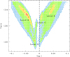 |
Fig. 7 ∆χ2 map in the (log s, log q) parameter plane of KMT-2023-BLG-1454. The notations and color coding of points are the same as those in Fig. 2. |
Solutions of KMT-2023-BLG-1642.
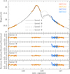 |
Fig. 8 Model curves of the three local solutions (A, B, and C) of KMT-2023-BLG-1454 in the region of the anomaly. The three lower panels show the residuals from the individual solutions. |
3.3 KMT-2023-BLG-1642
The source of the lensing event KMT-2023-BLG-1642 lies at the equatorial coordinates (RA, Dec) = (17:25:27.84, −29:03:30.49), which correspond to the Galactic coordinates (l, b) = (−2°.482, 3°.645). The source brightness at the baseline is Ibase = 19.34, and the extinction toward the field is AI = 1.87. The KMTNet group alerted the event at UT 02:28 on 2023 July 14, which corresponds to HJD′ = 140.1. The event reached its peak at HJD′ = 138.6 with a magnification Apeak ~ 12.5. The duration of the event is relatively short with an event time scale of te ~ 7 days.
Figure 10 displays the lensing light curve of KMT-2023-BLG-1642. Detailed inspection of the light curve revealed that there was an anomaly that occurred just before the event reached its peak. The anomaly lasted for about 1 day during 137.8 ≲ HJD′ ≲ 138.7. From the anomaly structure, which is characterized by two bumps centered at HJD′ ~ 137.85 and ~138.80 and the U-shaped trough between the bumps, it is likely that the anomaly was produced by the caustic crossings of the source through a tiny caustic induced by a lens companion. The early part of the first bump was not be covered because the KMTC site was clouded out on the night of the anomaly.
Figure 11 shows the ∆χ2 map on the log s–log q parameter plane constructed from the grid searches of the parameters. We identified three locals lying at (log s, log q) ~ (−0.01, −2.22) (local A), ~ (0.07, −1.98) (local B), and ~ (0.02, −2.46) (local C). The full lensing parameters of the individual local solutions determined after the refinement are listed in Table 3. The estimated mass ratios between the lens components are q ≲ 10−2 regardless of the solutions, indicating that the anomaly was produced by a companion having a planetary mass. In Fig. 12, we present the model curves of the three local solutions and residuals from the models. From the comparison of the goodness of the fits, it is found that the solution A is favored over the solutions B and C by ∆χ2 = 13.0 and 56.3, respectively. Considering the χ2 differences, the solution C is ruled out, but the solution B cannot be completely excluded. For the solutions A and B, the value  estimated from the lensing parameters approximately matches the geometric mean of the binary separations,
  , of the two solutions, and thus the similarity between the model curves is caused by the inner-outer degeneracy. In Fig. 11, we mark the geometric mean of sin and sout as a vertical dot-dashed line. The major difference between the model curves of the two solutions appears in the rising part of the first bump, but the incomplete coverage of the region makes it difficult to clearly lift the degeneracy between the solutions.
Figure 13 shows the lens-system configurations corresponding to the three local solutions. For all solutions, the caustics have a resonant form with connected planetary and central caustics. In the cases of the two solutions A and B, for which the lensing parameters except for the planet separation s are similar to each other, the source passes the outer and inner regions of the planetary caustic, respectively, indicating that the similarity between the model curves of the two solutions is caused by the inner–outer degeneracy. The lensing parameters (u0, tE, ρ) of the solution C are substantially different from those of the other solutions, and this indicates that the degeneracy between this and the other solutions is accidental, mostly because of the incomplete coverage of the anomaly.
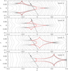 |
Fig. 9 Lens-system configurations of the three degenerate solutions (inner, outer, and intermediate solutions) of KMT-2023-BLG-1454. |
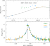 |
Fig. 10 Lensing light curve of KMT-2023-BLG-1642. |
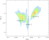 |
Fig. 11 ∆χ2 map in the (log s, log q) parameter plane of KMT-2023-BLG-1642. The color coding is set to represent points with ≤ 1rσ (red), ≤ 2nσ (yellow), ≤3nσ (green), and ≤ 4nσ (cyan), where n = 3. |
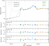 |
Fig. 12 Model curves and residuals from the three local solutions of KMT-2023-BLG-1642 in the region of the anomaly. |
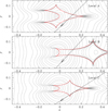 |
Fig. 13 Lens-system configurations of the three local solutions of KMT-2023-BLG-1642. |
4 Source stars and angular Einstein radii
In this section, we specify the source stars of the individual lensing events. Specifying the source of a lensing event is important not only to fully characterize the event but also to determine the angular Einstein radius, which is estimated by the relation
 (2)
(2)
where the normalized source radius is measured from the light curve modeling, and the angular source radius θ* can be deduced from the type of the source.
The source type is determined by measuring the reddening-and extinction-corrected (de-reddened) color and magnitude using the Yoo et al. (2004a) routine. In the first step of this routine, we measured the instrumental color and magnitude (V − I, I) of the source by regressing the I- and V-band datasets processed using the pyDIA photometry code with respect to the model lensing light curve, and then placed the source in the instrumental color-magnitude diagram (CMD) of stars lying near the source constructed with the use of the same pyDIA code. In the second step, we calibrated the color and magnitude of the source using the centroid of the red giant clump (RGC) as a reference, that is,
 (3)
(3)
Here (V − I, I)0 and (V − I, I)RGC,0 represent the de-reddened colors and magnitudes of the source and RGC centroid, respectively, and ∆(V − I, I) = (V − I, I) − (V − I, I)RGC represents the offsets in color and magnitude between the source and RGC centroid. The RGC centroid can be used as a reference for calibration because its de-reddened color and magnitude are known from Bensby et al. (2013) and Nataf et al. (2013), respectively.
In Fig. 14, we mark the position of the source star for each event and RGC centroid on the instrumental CMD. For KMT-2023-BLG-1454, the V-band magnitude of the source could not be measured due to the combination of the limited number of the V-band data points during the lensing magnification and the low quality of the data caused by the relatively severe extinction toward the field. In this case, we estimated the source color as the mean of colors of the stars lying in the giant or main-sequence branch of the combined ground+HST CMD with I-band magnitude offsets from the RGC centroid lying within the range of the measured value. The combined CMD was constructed by aligning the CMD established using KMTC data and that of stars in the Baade’s window observed with the use of the Hubble Space Telescope (Holtzman et al. 1998). In Table 4, we list the estimated values of (V − I, I), (V − I, I)RGC, (V − I, I)RGC,0, and the finally determined de-reddened source colors and magnitudes, (V − I, I)0, of the individual events. According to the estimated colors and magnitudes, the source star is a late G-type turnoff star for KMT-2023-BLG-0416, a K-type giant for KMT-2023-BLG-1454, and an early K-type subgiant star for KMT-2023-BLG-1642.
For the estimation of the angular Einstein radius from the relation in Eq. (2), we initially converted the V − I color into V − K color using the Bessell & Brett (1988) relation, and subsequently determined the angular source radius by applying the Kervella et al. (2004) relationship between V − K color and θ*.
With the estimated value of θE, the relative lens-source proper motion is computed using the measured event time scale as
 (4)
(4)
In Table 5, we list the estimated values of θ*, θE, and μ for the individual lensing events. For the events KMT-2023-BLG-0416 and KMT-2023-BLG-1642, the ρ value varies substantially over the local solutions, and thus we estimate θE and μ values corresponding to the individual local solutions.
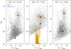 |
Fig. 14 Locations of source stars (marked by blue dots) with respect to the red giant clump (RGC) centroids (marked by red dots) for the lensing events KMT-2023-BLG-0416, KMT-2023-BLG-1454, and KMT-2023-BLG-1642 in the instrumental color-magnitude diagrams of stars lying near the source stars of the events. For KMT-2023-BLG-1454, the CMD is constructed by aligning the CMD established using KMTC data (grey dots) and that of stars in the Baade’s window (brown dots) observed with the use of the Hubble Space Telescope. |
Source parameters.
Einstein radii and relative lens-source proper motions.
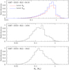 |
Fig. 15 Bayesian posteriors for the host masses of the planetary systems KMT-2023-BLG-0416L, KMT-2023-BLG-1454L, and KMT-2023-BLG-1642L. For KMT-2023-BLG-0416 and KMT-2023-BLG-1642 with varying θE values depending on local solutions, multiple posteriors corresponding to the individual solutions are presented. For these events, the relative probability is scaled by applying a factor exp(−∆χ2/2), where ∆χ2 denotes the difference in χ2 compared to the best-fit solution. The posterior of KMT-2023-BLG-1642 associated with the solution B is not prominently visible because of the very small scale factor. |
5 Physical lens parameters
In this section, we estimate the physical lens parameters of the individual events. The physical parameters of the lens mass M and distance DL are constrained from the lensing observables of tE, θE, and πE. Here πE indicates the microlens parallax, which is related to the relative lens-source parallax πrel = AU(1/Dl − 1/DS) and proper motion by
 (5)
(5)
where DS denotes the distance to the source. With the simultaneous measurements of all these observables, the mass and distance to the lens are uniquely determined by the Gould (2000) relation
 (6)
(6)
where κ = 4G/(c2AU) ≃ 8.14 mas/M⊙ and πS = AU]/DS denotes the parallax of the source. Among these lensing observables, the values of the event time scale and Einstein radius were securely measured for all events. The value of the microlens parallax can be measured from the subtle deviations in the lensing light curve induced by the digression of the relative lens-source motion from rectilinear caused by the orbital motion of Earth around the sun (Gould 1992). For none of the events, the microlens parallax can be measured because either the photometric precision of data is low or the event time scale is short. Nevertheless, the lens parameters can still be constrained because the other observables of tE and θE provide constraints on the mass and distance by the relations
 (7)
(7)
Therefore, we estimate the physical lens parameters by conducting Bayesian analyses with the constraints provided by tE and θE values of the individual events.
The Bayesian analysis was conducted according to the following procedure. In the first step of this process, we carried out a Monte Carlo simulation to generate a large number of synthetic lensing events, with the use of the prior information on the location, velocity, and mass function of astronomical objects within the Galaxy. In this simulation, we adopted the Jung et al. (2021) Galaxy model for the physical and dynamical distributions, and the Jung et al. (2022) model for the mass function of lens objects. Regarding KMT-2023-BLG-1454, the Gaia data archive (Gaia Collaboration 2018) contains information about the source, including its proper motion, but we have chosen not to include the Gaia proper motion value in our Monte Carlo simulation due to the substantial uncertainties associated with the source’s faintness. For each synthetic event produced from this simulation, we allocated the lens mass Mi, lens distance DL, i, source distance DS,i, and the lens-source transverse velocity v⊥,i, and then computed the corresponding lens observables using the relations tE, i = DL, iθE,i/v⊥,i and θE,i = (κMiπrel,i)1/2, and πrel,i = AU(1/DL,i − 1/DS,i). In the second step, we constructed posteriors of the lens mass and distance by assigning a weight to each synthetic event of
![${w_i} = \exp \left( { - {{{\chi ^2}} \over 2}} \right);\quad {\chi ^2} = \left[ {{{{{\left( {{t_{{\rm{E}},i}} - {t_{\rm{E}}}} \right)}^2}} \over {{\sigma ^2}\left( {{t_{\rm{E}}}} \right)}}} \right] + \left[ {{{{{\left( {{\theta _{{\rm{E}},i}} - {\theta _{\rm{E}}}} \right)}^2}} \over {{\sigma ^2}\left( {{\theta _{\rm{E}}}} \right)}}} \right].$](/articles/aa/full_html/2024/03/aa48245-23/aa48245-23-eq20.png) (8)
(8)
Here (te, θe) denote the measured values of the lensing observables, and [σ(tE), σ(θE)] represent their uncertainties.
In Figs. 15 and 16, we present the posteriors of the masses of the host stars and distances to the individual planetary systems. In the cases of KMT-2023-BLG-0416 and KMT-2023-BLG-1642, for which local solutions yield substantially divergent θE values, we constructed posteriors corresponding to the individual solutions. To represent these posteriors, we apply a scaling based on exp(−∆χ2/2), where ∆χ2 denotes the difference in χ2 compared to the best-fit solution. We point out that the scaling factors are ≲ 0.05 for the A solutions of KMT-2023-BLG-0416, ≲ 0.007 for the B, C, and D solutions of KMT-2023-BLG-1454, and ≲ 0.002 for the A solution of KMT-2023-BLG-1642, and thus the posteriors associated with these solutions are not presented. In Table 6, we list the estimated values of the host mass Mh, planet mass Mp = qMh, distance DL, and projected physical separation between the planet and host, a⊥ = sDlθe. For each physical parameter, we choose the median value of the posterior distribution as the representative value, and set the 16 and 84% of the posterior distribution as the lower and upper limits, respectively.
According to the Bayesian estimates, The estimated host mass of KMT-2023-BLG-0416L corresponds to a main-sequence star of a late K spectral type, and those of KMT-2023-BLG-1454L and KMT-2023-BLG-1642L correspond to that of a mid-M dwarf. In the case of the planetary system KMT-2023-BLG-0416L, the planet’s mass exhibits significant variation across solutions, ranging from approximately 6 times the mass of Jupiter according to A solutions, but resembling the mass of Uranus according to B solutions. In the case of the KMT-2023-BLG-1454L planetary system, the planet has a mass roughly half that of Jupiter, while in the case of the KMT-2023-BLG-1646L system, the planet exhibits a mass range of approximately 1.1–1.3 times that of Jupiter, categorizing both as giant planets.
Physical lens parameters.
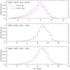 |
Fig. 16 Bayesian posteriors for the distances to the planetary systems KMT-2023-BLG-0416L, KMT-2023-BLG-1454L, and KMT-2023-BLG-1642L. Notations are the same as those in Fig. 15. |
6 Summary and conclusion
We presented the analyses of three lensing events KMT-2023-BLG-0416, KMT-2023-BLG-1454, and KMT-2023-BLG-1642, for which partially-covered short-term signals were found in their light curves from the investigation of the 2023 season data obtained from high-cadence microlensing surveys. Through these analyses, we identified that the signals in the analyzed lensing events were generated by planetary companions to the lenses.
Given the potential degeneracy caused by the partial coverage of the signals, we conducted a thorough exploration of the lensing parameter space. From the analysis of KMT-2023-BLG-0416, we have identified two distinct sets of solutions: one characterized by a mass ratio of approximately q ~ 10−2, and the other with q ~ 6.5 × 10⁻⁵, with each set yielding a pair of solutions caused by the inner-outer degeneracy. In the case of KMT-2023-BLG-1454, we have identified four distinct local solutions with mass ratios spanning in the range of q ~ (1.7−4.3) × 10−3. Among these solutions, two displayed resemblances in their model curves due to the inner-outer degeneracy, while the other two solutions arose due to accidental degeneracy. Regarding KMT-2023-BLG-1642, we have discerned two local solutions with mass ratios q ~ (6−10) × 10−3 arising from the inner-outer degeneracy.
We derived the physical lens parameters through Bayesian analyses, which incorporated constraints from the measured lensing observables of the event time scale and Einstein radius in conjunction with prior information regarding the density, velocity, and mass distribution of astronomical objects within our Galaxy. For KMT-2023-BLG-0416L planetary system, the host mass is ~0.6 M⊙ and the planet mass is ~(6.1−6.7) MJ according to one set of solutions and ~ 0.04 MJ according to the other set of solutions. KMT-2023-BLG-1454Lb has a mass roughly half that of Jupiter, while KMT-2023-BLG-1646Lb has a mass in the range of between 1.1 and 1.3 times that of Jupiter, classifying them both as giant planets orbiting mid M-dwarf host stars with masses ranging from 0.13 to 0.17 solar masses.
Acknowledgements
Work by C.H. was supported by the grants of National Research Foundation of Korea (2019R1A2C2085965). J.C.Y. acknowledges support from U.S. NSF Grant No. AST-2108414. Y.S. acknowledges support from BSF Grant No. 2020740. This research has made use of the KMTNet system operated by the Korea Astronomy and Space Science Institute (KASI) and the data were obtained at three host sites of CTIO in Chile, SAAO in South Africa, and SSO in Australia.
References
- Albrow, M. 2017, https://doi.org/10.5281/zenodo.268049 [Google Scholar]
- Albrow, M., Beaulieu, J.-P., Birch, P., et al. 1998, ApJ, 509, 687 [NASA ADS] [CrossRef] [Google Scholar]
- Albrow, M., Horne, K., Bramich, D. M., et al. 2009, MNRAS, 397, 2099 [Google Scholar]
- Alcock, C., Allsman, R. A., Axelrod, T. S., et al. 1995, ApJ, 445, 133 [NASA ADS] [CrossRef] [Google Scholar]
- Alcock, C., Allsman, R. A., Alves, D., et al. 1996, ApJ, 463, L67 [NASA ADS] [CrossRef] [Google Scholar]
- Alcock, C., Allen, W. H., Allsman, R. A., et al. 1997, ApJ, 491, 436 [Google Scholar]
- Bensby, T., Yee, J. C., Feltzing, S., et al. 2013, A&A, 549, A147 [NASA ADS] [CrossRef] [EDP Sciences] [Google Scholar]
- Bessell, M. S., & Brett, J. M. 1988, PASP, 100, 1134 [Google Scholar]
- Chung, S.-J., Han, C., Park, B.-G, et al. 2005, ApJ, 630, 535 [NASA ADS] [CrossRef] [Google Scholar]
- Doran, M., & Mueller, C. M. 2004, J. Cosmol. Astropart. Phys., 09, 003 [CrossRef] [Google Scholar]
- Erdl, H., & Schneider, P. 1993, A&A, 268, 453 [NASA ADS] [Google Scholar]
- Gaia Collaboration (Brown, A. G. A., et al.) 2018, A&A, 616, A1 [NASA ADS] [CrossRef] [EDP Sciences] [Google Scholar]
- Gaudi, B. S., 1998, ApJ, 506, 533 [Google Scholar]
- Gaudi, B. S., & Gould, A. 1997, ApJ, 486, 85 [Google Scholar]
- Gould, A. 1992, ApJ, 392, 442 [Google Scholar]
- Gould, A. 2000, ApJ, 542, 785 [NASA ADS] [CrossRef] [Google Scholar]
- Gould, A. 2022, arXiv e-prints [arXiv:2209.12501] [Google Scholar]
- Gould, A., & Loeb, A. 1992, ApJ, 396, 104 [Google Scholar]
- Gould, A., Dong, Subo, Gaudi, B. S., et al. 2010, ApJ, 720, 1073 [NASA ADS] [CrossRef] [Google Scholar]
- Gould, A., Han, C., Weicheng, Z., et al. 2022, A&A, 664, A13 [NASA ADS] [CrossRef] [EDP Sciences] [Google Scholar]
- Han, C. 2006, ApJ, 638, 1080 [Google Scholar]
- Han, C., Lee, C.-U., Zang, W., et al. 2023, A&A, 674, A90 [NASA ADS] [CrossRef] [EDP Sciences] [Google Scholar]
- Holtzman, J. A., Watson, A. M., Baum, W. A., et al. 1998, AJ, 115, 1946 [Google Scholar]
- Hwang, K.-H., Zang, W., Gould, A., et al. 2022, AJ, 163, 43 [NASA ADS] [CrossRef] [Google Scholar]
- Jung, Y. K., Udalski, A., Gould, A., et al. 2018, AJ, 155, 219 [Google Scholar]
- Jung, Y. K., Han, C., Udalski, A., et al. 2021, AJ, 161, 293 [NASA ADS] [CrossRef] [Google Scholar]
- Jung, Y. K., Zang, W., Han, C., et al. 2022, AJ, 164, 262 [NASA ADS] [CrossRef] [Google Scholar]
- Kervella, P., Thévenin, F., Di Folco, E., & Ségransan, D. 2004, A&A, 426, 29 [Google Scholar]
- Kim, S.-L., Lee, C.-U., Park, B.-G., et al. 2016, JKAS, 49, 37 [Google Scholar]
- Mao, S., & Paczynski, B., 1991, ApJ, 374, L37 [NASA ADS] [CrossRef] [Google Scholar]
- Nataf, D. M., Gould, A., Fouqué, P., et al. 2013, ApJ, 769, 88 [Google Scholar]
- Shin, I.-G., Yee, J. C., Zang, W., et al. 2023, AJ, 166, 104 [NASA ADS] [CrossRef] [Google Scholar]
- Tsapras, Y., Horne, K., Kane, S., & Carson, R. 2003, MNRAS, 343, 1131 [NASA ADS] [CrossRef] [Google Scholar]
- Udalski, A. 2003, Acta Astron., 53, 291 [NASA ADS] [Google Scholar]
- Udalski, A., Szymanski, M., Kaluzny, J., et al. 1993, Acta Astron., 43, 289 [NASA ADS] [Google Scholar]
- Udalski, A., Szymanski, M., Kaluzny, J., et al. 1994, Acta Astron., 44, 31 [Google Scholar]
- Yang, H., Yee, J. C., Hwang, K.-H., et al. 2023, MNRAS, 528, 11 [Google Scholar]
- Yee, J. C., Shvartzvald, Y., Gal-Yam, A., et al. 2012, ApJ, 755, 102 [Google Scholar]
- Yee, J. C., Zang, W., Udalski, A., et al. 2021, AJ, 162, 180 [NASA ADS] [CrossRef] [Google Scholar]
- Yoo, J., DePoy, D. L., Gal-Yam, A. et al. 2004a, ApJ, 603, 139 [Google Scholar]
- Yoo, J., DePoy, D. L., Gal-Yam, A., et al. 2004b, ApJ, 616, 1204 [NASA ADS] [CrossRef] [Google Scholar]
All Tables
All Figures
|
Fig. 1 Cumulative sum of χ2 for the individual datasets of the three analyzed events KMT-2023-BLG-0416, KMT-2023-BLG-1454, and KMT-2023-BLG-1642. The colors of the distributions match those of the datasets marked in the legend. |
| In the text | |
|
Fig. 2 Lensing light curve of KMT-2023-BLG-0416. The lower panel presents the overall perspective, while the upper panel provides a close-up view of the anomaly region. The arrow in the lower panel indicates the time of the anomaly. The curve drawn over the data points is a 1L 1S model obtained by fitting the light curve with the exclusion of the data around the anomaly. |
| In the text | |
|
Fig. 3 ∆χ2 map on the plane of the planet parameters (log s, log q) of the lensing event KMT-2023-BLG-0416. The color scheme represents points with ∆χ2 < 12n (red), < 22n (yellow), < 32n (green), and < 42n (cyan), where n = 2. The labels marked by Ain, Aout, Bin, and Bout represent positions of the four local solutions. The vertical dot-dashed line indicates the geometric mean between the binary separations of the Bin and Bout solutions. |
| In the text | |
|
Fig. 4 Model curves of the local solutions Aout and Bout for KMT-2023-BLG-0416. The lower panels show the residuals from the two local planetary solutions and the single-lens binary-source (1L2S) solution. |
| In the text | |
|
Fig. 5 Lens-system configurations of the four local solutions of KMT-2023-BLG-0416. In each panel, the red cuspy figure represents the caustic, the arrowed line is the source trajectory, and the grey curves surrounding the caustic represent the equi-magnification contours. |
| In the text | |
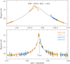 |
Fig. 6 Light curve of KMT-2023-BLG-1454. Notations are the same as those in Fig. 2. |
| In the text | |
|
Fig. 7 ∆χ2 map in the (log s, log q) parameter plane of KMT-2023-BLG-1454. The notations and color coding of points are the same as those in Fig. 2. |
| In the text | |
|
Fig. 8 Model curves of the three local solutions (A, B, and C) of KMT-2023-BLG-1454 in the region of the anomaly. The three lower panels show the residuals from the individual solutions. |
| In the text | |
|
Fig. 9 Lens-system configurations of the three degenerate solutions (inner, outer, and intermediate solutions) of KMT-2023-BLG-1454. |
| In the text | |
|
Fig. 10 Lensing light curve of KMT-2023-BLG-1642. |
| In the text | |
|
Fig. 11 ∆χ2 map in the (log s, log q) parameter plane of KMT-2023-BLG-1642. The color coding is set to represent points with ≤ 1rσ (red), ≤ 2nσ (yellow), ≤3nσ (green), and ≤ 4nσ (cyan), where n = 3. |
| In the text | |
|
Fig. 12 Model curves and residuals from the three local solutions of KMT-2023-BLG-1642 in the region of the anomaly. |
| In the text | |
|
Fig. 13 Lens-system configurations of the three local solutions of KMT-2023-BLG-1642. |
| In the text | |
|
Fig. 14 Locations of source stars (marked by blue dots) with respect to the red giant clump (RGC) centroids (marked by red dots) for the lensing events KMT-2023-BLG-0416, KMT-2023-BLG-1454, and KMT-2023-BLG-1642 in the instrumental color-magnitude diagrams of stars lying near the source stars of the events. For KMT-2023-BLG-1454, the CMD is constructed by aligning the CMD established using KMTC data (grey dots) and that of stars in the Baade’s window (brown dots) observed with the use of the Hubble Space Telescope. |
| In the text | |
|
Fig. 15 Bayesian posteriors for the host masses of the planetary systems KMT-2023-BLG-0416L, KMT-2023-BLG-1454L, and KMT-2023-BLG-1642L. For KMT-2023-BLG-0416 and KMT-2023-BLG-1642 with varying θE values depending on local solutions, multiple posteriors corresponding to the individual solutions are presented. For these events, the relative probability is scaled by applying a factor exp(−∆χ2/2), where ∆χ2 denotes the difference in χ2 compared to the best-fit solution. The posterior of KMT-2023-BLG-1642 associated with the solution B is not prominently visible because of the very small scale factor. |
| In the text | |
|
Fig. 16 Bayesian posteriors for the distances to the planetary systems KMT-2023-BLG-0416L, KMT-2023-BLG-1454L, and KMT-2023-BLG-1642L. Notations are the same as those in Fig. 15. |
| In the text | |
Current usage metrics show cumulative count of Article Views (full-text article views including HTML views, PDF and ePub downloads, according to the available data) and Abstracts Views on Vision4Press platform.
Data correspond to usage on the plateform after 2015. The current usage metrics is available 48-96 hours after online publication and is updated daily on week days.
Initial download of the metrics may take a while.