| Issue |
A&A
Volume 683, March 2024
|
|
|---|---|---|
| Article Number | A115 | |
| Number of page(s) | 11 | |
| Section | Planets and planetary systems | |
| DOI | https://doi.org/10.1051/0004-6361/202347951 | |
| Published online | 12 March 2024 | |
Three sub-Jovian-mass microlensing planets: MOA-2022-BLG-563Lb, KMT-2023-BLG-0469Lb, and KMT-2023-BLG-0735Lb
1
Department of Physics, Chungbuk National University,
Cheongju
28644, Republic of Korea
e-mail: This email address is being protected from spambots. You need JavaScript enabled to view it.
2
Korea Astronomy and Space Science Institute,
Daejon
34055, Republic of Korea
3
Korea University of Science and Technology, Korea, (UST),
217 Gajeong-ro, Yuseong-gu,
Daejeon
34113, Republic of Korea
4
Institute of Natural and Mathematical Science, Massey University,
Auckland
0745, New Zealand
5
Max-Planck-Institute for Astronomy,
Königstuhl 17,
69117
Heidelberg, Germany
6
Department of Astronomy, Ohio State University,
140 W. 18th Ave.,
Columbus,
OH
43210, USA
7
University of Canterbury, Department of Physics and Astronomy,
Private Bag 4800,
Christchurch
8020, New Zealand
8
Center for Astrophysics | Harvard & Smithsonian,
60 Garden St.,
Cambridge, MA
02138, USA
9
Department of Particle Physics and Astrophysics, Weizmann Institute of Science,
Rehovot
76100, Israel
10
Department of Astronomy, Tsinghua University,
Beijing
100084, PR China
11
School of Space Research, Kyung Hee University,
Yongin, Kyeonggi
17104, Republic of Korea
12
Institute for Space-Earth Environmental Research, Nagoya University,
Nagoya
464-8601, Japan
13
Code 667, NASA Goddard Space Flight Center,
Greenbelt, MD
20771, USA
14
Department of Astronomy, University of Maryland,
College Park, MD
20742, USA
15
Department of Earth and Planetary Science, Graduate School of Science, The University of Tokyo,
7-3-1 Hongo, Bunkyo-ku,
Tokyo
113-0033, Japan
16
Instituto de Astrofísica de Canarias,
Vía Láctea s/n,
38205
La Laguna, Tenerife, Spain
17
Department of Earth and Space Science, Graduate School of Science, Osaka University,
Toyonaka, Osaka
560-0043, Japan
18
Department of Physics, The Catholic University of America,
Washington, DC
20064, USA
19
Institute of Space and Astronautical Science, Japan Aerospace Exploration Agency,
3-1-1 Yoshinodai, Chuo, Sagamihara,
Kanagawa
252-5210, Japan
20
Sorbonne Université, CNRS, UMR 7095, Institut d’Astrophysique de Paris,
98 bis bd Arago,
75014
Paris, France
21
Department of Physics, University of Auckland,
Private Bag 92019,
Auckland, New Zealand
22
University of Canterbury Mt. John Observatory,
PO Box 56,
Lake Tekapo
8770, New Zealand
Received:
12
September
2023
Accepted:
19
January
2024
Abstract
Aims. We analyze the anomalies appearing in the light curves of the three microlensing events MOA-2022-BLG-563, KMT-2023-BLG-0469, and KMT-2023-BLG-0735. The anomalies exhibit common short-term dip features that appear near the peak.
Methods. From the detailed analyses of the light curves, we find that the anomalies were produced by planets accompanied by the lenses of the events. For all three events, the estimated mass ratios between the planet and host are on the order of 10−4: q ~ 8 × 10⁻⁴ for MOA-2022-BLG-563L, q ~ 2.5 × 10⁻⁴ for KMT-2023-BLG-0469L, and q ~ 1.9 × 10⁻⁴ for KMT-2023-BLG-0735L. The interpretations of the anomalies are subject to a common inner-outer degeneracy, which causes ambiguity when estimating the projected planet-host separation.
Results. We estimated the planet mass, Mp, host mass, Mh, and distance, DL, to the planetary system by conducting Bayesian analyses using the observables of the events. The estimated physical parameters of the planetary systems are (Mh/M⊙, Mp/MJ, DL/kpc) = (0.48−0.30+0.36, 0.40−0.25+0.31, 6.53−1.57+1.12) for MOA-2022-BLG-563L, (0.47−0.26+0.35, 0.124−0.067+0.092, 7.07−1.19+1.03) for KMT-2023-BLG-0469L, and (0.62−0.35+0.34, 0.125−0.070+0.068, 6.26−1.67+1.27) for KMT-2023-BLG-0735L. According to the estimated parameters, all planets are cold planets with projected separations that are greater than the snow lines of the planetary systems, they have masses that lie between the masses of Uranus and Jupiter of the Solar System, and the hosts of the planets are main-sequence stars that are less massive than the Sun. In all cases, the planetary systems are more likely to be in the bulge with probabilities Pbulge = 64%, 73%, and 56% for MOA-2022-BLG-563, KMT-2023-BLG-0469, and KMT-2023-BLG-0735, respectively.
Key words: gravitation / gravitational lensing: micro / planets and satellites: detection
© The Authors 2024
 Open Access article, published by EDP Sciences, under the terms of the Creative Commons Attribution License (https://creativecommons.org/licenses/by/4.0), which permits unrestricted use, distribution, and reproduction in any medium, provided the original work is properly cited.
This article is published in open access under the Subscribe to Open model. This email address is being protected from spambots. You need JavaScript enabled to view it. to support open access publication.
1 Introduction
Because of its trait that does not depend on the luminosity of a lensing object, microlensing provides an important tool to detect extrasolar planets. Planetary microlensing (Mao & Paczynski 1991; Gould & Loeb 1992) was proposed before the first discoveries of an exoplanet belonging to a pulsar (Wolszczan & Frail 1992) and a planet belonging to a normal stellar system (Mayor & Queloz 1995), but the first microlensing planet was only discovered in 2004 (Bond et al. 2004), that is, 12 yr after the operation of the first-generation microlensing surveys, for example, Massive Compact Halo Objects (MACHO: Alcock et al. 1993), Optical Gravitational Lensing Experiment (OGLE: Udalski et al. 1994), and Expérience pour la Recherche d’Objets Sombres (EROS: Aubourg et al. 1993). The difficulty of finding planets from these early microlensing surveys was mostly ascribed to the low cadence of the surveys, which were typically carried out with a 1 day cadence, while the duration of a planet-induced lensing signal is several hours for terrestrial planets and several days even for giant planets. In order to increase the observational cadence, planetary microlensing experiments during the time from the mid 1990s to mid 2010s had been carried out in a hybrid mode (Gould & Loeb 1992; Albrow et al. 1998), in which survey experiments with a low observational cadence mainly focused on detecting lensing events, and follow-up groups conducted high-cadence observations for a fraction of events detected by the survey experiments.
Planetary microlensing experiments entered a new phase in the mid 2010s by dramatically increasing the observational cadence of lensing surveys with the employment of globally distributed multiple telescopes that are equipped with very wide-field cameras. With the upgraded instrument, the current lensing surveys achieve observational cadences down to 0.25 h, which is two orders of magnitude shorter than the cadence of the early experiments. The operation of the high-cadence surveys has led to the great increase in the event detection rate, and the number of lensing events that are annually detected by the current lensing surveys is more than 3000, which is nearly two orders of magnitude higher than the rate of the early surveys. Being able to monitor a large number of lensing events with enhanced cadences, the detection rate of planets has also greatly increased. According to the NASA Exoplanet Archive1, the number of microlensing planets that have been detected since the full operation of the high-cadence surveys in 2016 is 137, and this is more than two times the 64 planets found from the previous experiments that had been conducted for 24 yr from the year 1992 to 2015. Considering that the high-cadence surveys were partially operated in 2020 due to the COVID pandemic and the data collected in the 2022 and 2023 season are under analysis, the current surveys are annually detecting about 30 planets on average (Gould et al. 2022; Jung et al. 2022).
The growing number of microlensing planets reveals similar anomaly patterns in certain planetary signals. Han et al. (2021a) outlined instances of planetary signals emerging via a non-caustic-crossing channel in their analysis of two lensing events KMT-2022-BLG-0475 and KMT-2022-BLG-1480. Similarly, Han et al. (2021a) depicted analogous occurrences of non-caustic-crossing signals in their study of the three planetary lensing events KMT-2018-BLG-1976, KMT-2018-BLG-1996, and OGLE-2019-BLG-0954. In their examination of the three planetary events KMT-2017-BLG-2509, OGLE-2017-BLG-1099, and OGLE-2019-BLG-0299, Han et al. (2021a) presented various instances where planetary signals emerged from source crossings over resonant caustics formed by giant planets near the Einstein rings of host stars. Jung et al. (2021) demonstrated planetary signals arising from perturbations by peripheral caustics induced by planets in their analyses of two lensing events OGLE-2018-BLG-0567 and OGLE-2018-BLG-0962. Moreover, in the cases of KMT-2018-BLG-1743 and KMT-2021-BLG-1898, Han et al. (2021b) and Han et al. (2022), respectively, highlighted two microlensing planets with signals deformed by companions to the source stars. Additionally, Han et al. (2017) presented an exemplary case of a planetary signal arising through a repeating channel from the analysis of the microlensing planet OGLE-2016-BLG-0263Lb. These various studies collectively underscore the diverse mechanisms and complexities observed in detecting microlensing planets.
Microlensing planets are found from detailed analyses of anomalous signals appearing in numerous lensing light curves. These analyses are done via a complex procedure and require heavy computations in order to identify the planetary origin of signals by distinguishing them from signals of other origins. Therefore, morphological studies by classifying lensing events with similar anomalies and investigating the origins for the individual classes of anomalies are important not only for the diagnosis of anomalies before detailed analysis but also for the accurate characterization of lens systems for future lensing events with similar anomaly structures.
In this work, we conduct analyses of the three compiled planetary microlensing events that were detected from short-term signals exhibiting similar anomaly features, including MOA-2022-BLG-563 KMT-2023-BLG-0469 and KMT-2023-BLG-0735. These events share similar characteristics, in which the anomalies showed up near the peaks of the lensing light curves and they exhibit similar dip features surrounded by peaks on both sides of the dips. We present the common characteristics of the planetary systems that are found from the detailed analyses of the anomalies.
We present the analyses of the lensing events according to the following organization. In Sect. 2, we describe the observations conducted to acquire the data used in the analyses, and mention the instruments used for the observations and the procedure of data reduction and error-bar normalization. In Sect. 3, we begin by briefly mentioning planetary lensing properties and introducing parameters used in the modeling of the lensing light curves. In the subsequent subsections, we present detailed analyses conducted for the individual events: in Sect. 3.1 for MOA-2022-BLG-563, in Sect. 3.2 for KMT-2023-BLG-0469, and in Sect. 3.3 for KMT-2023-BLG-0735. In Sect. 4, we characterize the source stars of the events and estimate the angular Einstein radii. In Sect. 5, we determine the physical parameters of the planetary system by conducting Bayesian analyses for the individual events. We summarize the results found from the analyses and conclude in Sect. 6.
Coordinates, baseline magnitude, and extinction.
2 Observations and data
The anomalous nature of the three lensing events MOA-2022-BLG-563, KMT-2023-BLG-0469, and KMT-2023-BLG-0735 were found from the inspection of the data obtained from the two high-cadence lensing surveys conducted toward the Galactic bulge field by the Korea Microlensing Telescope Network (KMTNet: Kim et al. 2016) group and the Microlensing Observations in Astrophysics (MOA: Bond et al. 2001) group. Among these events, KMT-2023-BLG-0469 and KMT-2023-BLG-0735 were observed solely by the KMTNet group, and MOA-2022-BLG-563 was observed by both survey groups. The KMTNet ID reference corresponding to the event MOA-2022-BLG-563 is KMT-2022-BLG-2681, and, hereafter, we use the MOA ID reference because the event was first discovered by the MOA group. In Table 1, we list the equatorial and galactic coordinates of the events together with the I-band baseline magnitudes, Ibase, and extinction, AI, toward the source stars. The ,-band extinction is estimated as AI = 7 AK, where the K-band extinction AK is adopted from Gonzalez et al. (2012).
The KMTNet observations of the events were carried out using three identical 1.6 m telescopes, which are globally distributed in the three continents of the Southern Hemisphere: at the Cerro Tololo Inter-American Observatory in Chile, the South African Astronomical Observatory in South Africa, and the Siding Spring Observatory in Australia. We designate the individual KMTNet telescopes as KMTC, KMTS, and KMTA using the initials of the countries in which the telescopes are located. The MOA observations were done using the 1.8 m telescope of the Mt. John Observatory located in New Zealand. The fields of view of the cameras mounted on the KMTNet telescopes and the MOA telescope are 4 deg2 and 2.2 deg2, respectively. We describe details of the observations conducted for the individual events in the following section.
Reduction of images and photometry of the source stars were carried out using the photometry codes of the individual groups, which were developed by Albrow et al. (2009) for the KMTNet survey and by Bond et al. (2001) for the MOA survey. For a fraction of the KMTC data set, additional photometry using the pyDIA code (Albrow et al. 2017) was done to construct color-magnitude diagram (CMD) of stars lying near the source stars and to determine the source colors. For the data used in the analyses, the error bars estimated from the photometry pipelines were readjusted so that they are consistent with the scatter of the data and χ2 per degree of freedom (dof) for each data set becomes unity. This error-bar normalization process was done following the routine depicted in detail by Yee et al. (2012).
3 Anomaly analysis
The image of a microlensed source star is split into two, in which the brighter one (major image) appears outside of the Einstein ring, and the fainter one (minor image) appears inside the ring. Planet-induced anomalies in a lensing light curve arise when a planet lies close to one of these two source images. The “major-image perturbation” refers to the case in which the planet perturbs the major image, and the “minor-image perturbation” indicates the case in which the planet perturbs the minor image (Gaudi & Gould 1997). When the planet perturbs the major image, the image is further magnified by the planet, and this results in a bump feature (positive deviations) of the anomaly. When the planet disturbs the minor image, by contrast, the image is demagnified, and this results in a dip feature (negative deviations) of the anomaly. Because the major image lies outside the Einstein ring, the bump feature of a planetary anomaly is generally produced by a “wide planet”, for which the projected planet-host separation is greater than the Einstein radius. By contrast, the dip feature of an anomaly is generated by a “close planet”, for which the separation is smaller than the Einstein radius, because the minor image lies inside the Einstein ring. See the appendix of Han et al. (2018) for more detailed discussion on the types of planetary perturbations.
As viewed on the source plane, planet-induced anomalies arise when the source approaches the planet-induced caustics. Caustics refer to the source positions at which the lensing magnifications of a point source are infinite. Planet-induced caustics form two sets of caustics, in which the “central caustic” forms near the position of the planet host, and the “planetary caustic” forms away from the host at the position ~(1 − 1/s2)s. Here s denotes the position vector of the planet from the host with a length normalized to the angular Einstein radius θE of the planetary lens system. For detailed descriptions on the position, size, and shape of the central and planetary caustics, see Chung et al. (2005) and Han (2006).
There exist multiple known channels that can produce short-term anomalies in lensing light curves. Besides the planetary channel, it is known that bump-featured anomalies can be produced via a 1L2S channel, in which the lens system is composed of a single-mass lens and binary source, and the bump feature can be generated by the close approach of the faint source companion to the lens (Gaudi et al. 1998). Dip-featured anomalies can be produced not only by a planet but also by a binary companion to the lens, although the two features can be usually distinguished from the shape of the dip feature (Han & Gaudi 2008).
The events analyzed in this work share a common characteristics that short-term anomalies with dip features appear near the peaks of the lensing light curves. Considering that a dip-featured anomaly is produced by a lens with either a binary companion or a planet, we conduct a binary-lens single-source (2L1S) modeling of the light curves for the interpretations of the observed anomalies. For each lensing event, the modeling was done in search of a lensing solution, which refers to a set of the lensing parameters that define the light curve of the event. Under the approximation of the rectilinear relative motion between the lens and source, the light curve of a 2L1S event is characterized by 7 lensing parameters. The first set of the three parameters (t0, u0, tE) define the source approach to the lens, and the individual parameters denote the time of the closest lens-source approach, the separation at that time (impact parameter), and the event time scale, respectively. The second set of the three parameters (s, q, α) define the binary lens, and the first two parameters represent the projected separation and mass ratio between the binary-lens components (M1 and M2), respectively, and the other parameter denotes the angle (source trajectory angle) between the direction of the relative lens-source proper motion vector µ and the M1−M2 axis. The lengths of u0 and s are scaled to the Einstein radius. The last parameter ρ is defined as the ratio of the angular source radius θ*, to the Einstein radius, that is, ρ = θ*/θE (normalized source radius), and it describes the deformation of a lensing light curve by finite-source effects during source crossings over caustics or close approaches to caustics.
Among the lensing parameters, we search for the binary parameters s and q via a grid approach with multiple starting values of α, and find the other parameters via a downhill approach. In the downhill approach, χ2 is minimized using the Markov chain Monte Carlo (MCMC) method with an adaptive step size Gaussian sampler (Doran & Mueller 2004). We then refine the local solutions appearing in the ∆χ2 map on the plane of the grid parameters, and then find a global solution by comparing the χ2 values of the individual local solutions. The anomalies of the all analyzed events appear near the peaks of the lensing light curves. Such central anomalies are known to be produced by a planetary companion lying around the Einstein ring of the planet host or a very close or wide binary companion to the primary lens. In order to check both the planetary and binary origins of the anomalies, we set the ranges of the grid wide enough to check both possible origins of the anomalies: −1.0 < log s < 1.0 and −5.0 < log q < 1.0. For the case that multiple solutions with similar χ2 values exist, we present all degenerate solutions.
In the following subsections, we present the analyses conducted for the individual events. We describe in detail the features of the anomalies residing in the light curves and present the results found from the modeling. For events with multiple identified solutions, we explain the cause of the degeneracy among the solutions.
3.1 MOA-2022-BLG-563
The lensing event MOA-2022-BLG-563 was first found on 2022 October 14, which corresponds to the abridged Heliocentric Julian day HJD′ = HJD − 2450000 ~ 9866, by the MOA group, and was later identified by the KMTNet group from the postseason analysis of the 2022 season data (Kim et al. 2018). The source position of the event corresponds to the KMTNet prime fields of BLG03 and BLG43, toward which observations were conducted with a 0.5 h cadence for each field and a 0.25 h cadence in combination. The MOA observations were conducted with a similar cadence. The event occurred during the late stage of the 2022 bulge season, and thus the declining part of the light curve after HJD′ ~ 9878 could not be covered. The source brightness returned to the baseline in the beginning of the 2023 season, and thus we do not include the 2023 season data in the analysis. We included the KMTC V-band data in the analysis because one data point lies in the region of the anomaly. Although the event lies in the field that usually is observed frequently, there are gaps among the data sets because of the short duration of observation time at the late stage of the bulge season.
The lensing light curve of MOA-2022-BLG-563 is shown in Fig. 1. The event reached a moderate magnification of Amax ~ 5.5 at the peak. From the inspection of the light curve, we find that the peak region of the light curve displays a short-term deviation from a single-lens single-source (1L1S) model. The anomaly is characterized by a dip feature centered at HJD′ ~ 9871.5 and double peaks lying on both sides of the dip. The time gap between the peaks is about 0.8 day. The dip part of the anomaly was covered by the KMTC data, and the peaks were covered by the MOA data. Besides these main features, the data before and after the peaks show weak positive deviations from the 1L1S model.
From the modeling of the light curve, it was found that the anomaly was produced by a planetary companion to the lens.
We identified a pair of degenerate solutions with binary parameters (log s, log q)in ~ (−0.050,−3.1) and (log s, log q)out ~ (−0.005, −3.1). The top panel of Fig. 2 shows the positions of the two local solutions in the ∆χ2 map on the (log s, log q) parameter plane. For the reason discussed below, we designate the former and latter solutions as “inner” and “outer” solutions, respectively. In Table 2, we list the full lensing parameters of the inner and outer solutions together with χ2 values of the fits and degrees of freedom (dof). The two solutions are very degenerate, and the inner solution is favored over the outer solution by only ∆χ2 = 1.0. The model curve of the inner solution is drawn over the data points in Fig. 1, and the residuals from the inner 2L1S and ILI S solutions in the region around the anomaly are shown in the lower two panels.
The upper and lower panels of Fig. 3 show the lens-system configurations of the inner and outer solutions, respectively. The configurations show that the source passed the region between the central and planetary caustics according to the inner solution, while the source passed the region outside the caustic according to the outer solution. The planetary and central caustics of the inner solution are well separated, while the two sets of caustics of the outer solution merge together and form a single resonant caustic. The dip feature of the anomaly was produced when the source passed through the negative deviation region on the back-end side of the caustic, and the bump features were produced when the source went through the positive deviation region extending from the strong cusps of the caustic. The normalized source radius ρ could have been measured if the event had occurred in mid-season, so that there would be dense coverage over the cusp approach, but the large gaps among the data sets together with the non-caustic-crossing nature of the anomaly features made it difficult to measure ρ.
We find that the degeneracy between the two solutions originates from the “inner-outer” degeneracy. This degeneracy was originally introduced by Gaudi & Gould (1997) to point out the similarity between the planetary signals resulting from the source passages through the near (inner) and far (outer) sides of the planetary caustic. Yee et al. (2021) pointed out the continuous transition between the inner-outer and close-wide degeneracies, where the latter degeneracy originates from the similarity between the central caustics induced by a pair of planets with separation s and 1/s (Griest & Safizadeh 1998; Dominik 1999; An 2005). While the planetary separations of the pair of solutions that are subject to the close-wide degeneracy follows the relation sclose × swide = 1, the planetary separations of the pair of solutions that are subject to the inner-outer degeneracy, sin and sout, follow the relation
 (1)
(1)
where  , τanom = (tanom— t0)/tE tanom indiCates the time of the anomaly, and the signs in the right term are “+” and “−” for the anomalies that are generated by the major and minor images perturbations, respectively (Hwang et al. 2022; Gould et al. 2022). We note that for uanom → 0, we have
  , which recovers the high-magnification limit of Griest & Safizadeh (1998). In the case of MOA-2022-BLG-563, the sign is “−” because the anomaly displayed a dip feature produced by the minor-image perturbation. With the lensing parameters (t0,u0,tE,tanom) ~ (9872.226,0.123,19.6,9871.3), we find s† ~ 0.936, and this matches very well the geometric mean (sin × sout)1/2 ~ 0.935. In the top panel of Fig. 2, we mark the s† as a dashed vertical line.
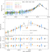 |
Fig. 1 Light curve of MOA-2022-BLG-563. The top panel shows the whole view, and the lower panels show the zoom-in view around the anomaly and the residuals from the 2L1S and ILI S models. The solid and dashed curves drawn over the data points are the 2L1S and ILI S models, respectively. The colors of data points are set to match the labels of the observatories in the legend. |
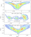 |
Fig. 2 ∆χ2 maps on the (log s, log q) parameter plane for the events MOA-2022-BLG-563 (top panel), KMT-2023-BLG-0469 (middle panel), and KMT-2023-BLG-0735 (bottom panel). Color coding is set to indicate points with ∆χ2 ≤ 12n (red), ≤22n (yellow), <32n (green), ≤42n (cyan), and ≤52n (blue), where n = 2. The dashed vertical line in each panel represents the geometric mean, (sin × sout)1/2, of the planet separations of the inner and outer solutions. |
Model parameters of MOA-2022-BLG-563.
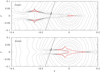 |
Fig. 3 Lens-system configurations of MOA-2022-BLG-563. The configurations of the inner and outer solutions are shown in the upper and lower panels, respectively. In each panel, the red figures represent the caustics, and the arrowed line is the source trajectory. Gray contours encompassing the caustics represent equi-magnification contours. The coordinates are centered at the center of mass of the planetary lens system, and the lengths are scaled to the Einstein radius. |
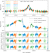 |
Fig. 4 Light curve of KMT-2023-BLG-0469. The solid, dotted, and dashed curves on the data points represent the models of the outer, intermediate, and inner 2L1S solutions, respectively. |
3.2 KMT-2023-BLG-0469
The lensing event KMT-2023-BLG-0469 was discovered by the KMTNet group on 2023 April 18 (HJD′ ~ 10052), near which the event reached its maximum magnification of Amax ~ 120. The source of the event lies in a small (0.8 deg2) region that is covered by the four KMTNet prime fields BLG02, BLG03, BLG42, and BLG43, and thus the event was observed very densely with a combined cadence of 0.125 h. See the layout of the KMTNet fields presented in Fig. 12 of Kim et al. (2018). As we discuss in Sect. 4, the source is very faint and the baseline flux is heavily blended. As a result, the source at the peak was brighter than the baseline by only ~1.1 mag despite the high magnification of the event.
The lensing light curve of KMT-2023-BLG-0469 is shown in Fig. 4, in which the top panel shows the whole view, and the second panel shows the zoom-in view of the anomaly region appearing near the peak. Similar to the case of MOA-2022-BLG-563, the anomaly is characterized by a dip feature and the positive peaks appearing before and after the dip. The anomaly is centered at tanom ~ 10 052.8 in HJD′, and the time gap between the two peaks is ~1.2 days. The second half of the first peak, which was covered by the KMTS data sets, exhibits a sharply declining feature, indicating that the peak was produced by the caustic crossing of the source. On the other hand, the second peak exhibits a smoothly varying feature, suggesting that the peak was produced by the cusp approach of the source.
From the analysis of the lensing light curve, we find that KMT-2023-BLG-0469 share common properties to those of the event MOA-2022-BLG-563 in the sense that the anomaly was produced by a low-mass planetary companion and the solution is subject to the inner-outer degeneracy. The planetary parameters of the inner and outer solutions are (s, q)in ~ (0.95,2.6 × 10−4) and (s, q)out ~ (1.03,2.5 × 10−4), respectively. Regardless of the solutions, the estimated planet-to-host mass ratio is much smaller than the Jupiter/Sun mass ratio of ~10−3, and this suggests that the planet is less massive than Jupiter. We list the full lensing parameters of the two solutions in Table 3. With the lensing parameters (t0, u0, tE, tanom) ~ (10052.07,8.42 × 10−3,44.6,10052.8), we find s† = 0.991, which matches well the geometric mean (sin × sout)1/2 ~ 0.989, and this indicates that the degeneracy between the two solutions is caused by the inner-outer degeneracy. We mark the position of s† on the Δχ2 map presented in the middle panel of Fig. 2.
Besides the two solutions resulting from the inner-outer degeneracy, we found an additional degenerate solution. The Δχ2 map presented in the middle panel of Fig. 2 shows the three local solutions. The additional solution has binary parameters (s, q)int ~ (0.98,2.1 × 10−4). We designate this solution as “intermediate” solution because the planet separation of the solution approximately corresponds to the mean of the inner and outer solutions. We list the full lensing parameters of the intermediate solution in Table 3. Among the three degenerate solutions, the outer solution is preferred over the inner and intermediate solutions by Δχ2 = 12.3 and 24.3, respectively. In Fig. 4, we plot the model curves and residuals of the outer (solid curve), intermediate (dotted curve), and inner (dashed curve) solutions.
In Fig. 5, we present the lens-system configurations corresponding to the three degenerate solutions. The configurations of the pair of the inner and outer solutions have similar characteristic to those of the event MOA-2022-BLG-563: the source passed through the inner region between the central and planetary caustics for the inner solution, and the source passed through the region outside the caustic for the outer solution. For the intermediate solution, on the other hand, the source passed through the two caustic prongs that extend from the two back-end cusps of a resonant caustic. According to this solution, the source crossed the caustic four times during the anomaly. The first pair of crossings occurred when the source passed through the lower prong, and the other pair of crossings occurred when the source passed through the upper prong. The individual caustic crossings produced caustic spikes, but the one produced when the source entered the lower caustic prong and the one generated when the source exited the upper caustic prong do not exhibit obvious features due to the combination of the weakness of the caustic folds and finite-source effects. From the resolved caustic-crossing part of the anomaly, the normalized source radius, ρ = (0.674 ± 0.038) × 10−3, is precisely measured.
Model parameters of KMT-2023-BLG-0469.
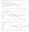 |
Fig. 5 Lens-system configurations of the inner (top panel), intermediate (middle panel), and outer (bottom panel) solutions for the lensing event KMT-2023-BLG-0469. Notations are same as those in Fig. 3. |
3.3 KMT-2023-BLG-0735
The KMTNet group found the event KMT-2023-BLG-0735 on 2023 May 08 (HJD′ ~ 10 072), which was about two days after the peak of the lensing light curve. The event reached a moderately high magnification of Amax ~ 60 at the peak. The extinction toward the source, AI = 5.97, is very high because of the closeness of the source to the Galactic center. The source lies near the edge of the KMTNet prime fields BLG02 and BLG42. The KMTC data were recovered from the images of both fields, but the KMTS and KMTA data in the BLG42 field were not recovered. As a result, the observational cadence varies depending on the field: 0.25 h for the KMTC data set and 0.5 h for the KMTS and KMTA data sets.
We present the lensing light curve of KMT-2023-BLG-0735 in Fig. 6. The light curve exhibits similar characteristics to those of the previous two events in various aspects. First, an anomaly occurred near the peak of the light curve. Second, the anomaly exhibits a dip feature, which is centered at tanom ~ 10 070.84 in HJD′, and two positive peaks on both sides of the dip. The time gap between the two peak is Δt ~ 0.6 day. The anomaly was covered mostly by the combination of KMTC02 and KMTC42 data sets
As expected from the similar pattern of the anomaly to those of MOA-2022-BLG-563 and KMT-2023-BLG-0469, we find a pair of inner and outer planetary solutions describing the observed anomaly. The planetary parameters are (s, q)in ~ (0.95,2.6 × 10−4) for the inner solution and (s, q)out ~ (1.03,2.5 × 10−4) for the outer solution, and the estimated mass ratio indicates that the planet is likely to be substantially less massive than Jupiter of the Solar System. The positions of the two degenerate solutions in the log s-log q parameter plane are shown on the Δχ2 map presented in the bottom panel of Fig. 2, and the full lensing parameters of both solutions are listed in Table 4. The two solutions are very degenerate, and the outer solution is preferred over the inner solution only by Δχ2 = 0.8. From the lensing parameters (t0, u0, tE, tanom) ~ (10070.61,1.75 × 10−2,18.5,10070.84), we find s† ~ 0.98 compared to the geometric mean (sin × sout)1/2 ~ 0.97, indicating that the degeneracy between the solutions is caused by the inner-outer degeneracy. The model curve of the outer solution and the residual are shown in Fig. 6.
Figure 7 shows the lens-system configurations corresponding to the inner and outer solutions of KMT-2023-BLG-0735. According to the configurations, the anomaly was produced by the passage of the source through the negative deviation region on the back-end side of the caustic. The configurations are very similar to those of the MOA-2022-BLG-563 in the senses that the ambiguity between the two solutions originates from the inner-outer degeneracy, and the central and planetary caustics of the inner solution are well separated, while the caustics of the outer solution form a single resonant caustic. Although the source did not cross the caustic, the normalized source radius, ρ = (1.64 ± 0.53) × 10−3, is measured because of the large magnification gradient of the anomaly region extending from the strong cusp of the caustic.
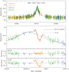 |
Fig. 6 Light curve of KMT-2023-BLG-0735. |
Model parameters of KMT-2023-BLG-0735.
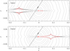 |
Fig. 7 Lens-system configurations of the inner (upper panel) and outer (lower panel) solutions for the lensing event KMT-2023-BLG-0735. Notations are same as those in Fig. 3. |
4 Source star and Einstein radius
In this section, we characterize the source stars of the events and estimate the angular Einstein radii. The Einstein radius is estimated from the relation
 (2)
(2)
where the normalized source radius ρ is measured from the light curve modeling, and the angular source radius θ* is deduced from the type of the source determined from its extinction and reddening-corrected (dereddened) color and magnitude. Although the angular Einstein radius cannot be estimated for MOA-2022-BLG-563 because the normalized source radius could not measured, we specify the source star for the complete characterization of the event.
For each event, the dereddened color and magnitude of the source, (V – I, I)0, were estimated using the Yoo et al. (2004) method. In this method, the instrumental color and magnitude, (V – I, I), of the source are measured, and then they are calibrated using the centroid of red giant clump (RGC), for which its dereddened values, (V – I, I)rgc,0, are known, as a reference, that is,
 (3)
(3)
Here Δ(V – I, I) represents the offsets in color and magnitude between the source and RGC centroid. The instrumental V and I-band magnitudes of the source were measured by regressing the light curves of the individual passbands constructed using the pyDIA photometry code (Albrow et al. 2017) with respect to the model.
For KMT-2023-BLG-0735, the photometry quality of the V-band data is not good because of the very high extinction toward the field, and this makes it difficult to directly measure the source color. In this case, we adopted the median color of stars lying within the range of the measured I-band magnitude on the main-sequence or giant branches of the combined CMD, which is constructed by aligning the CMD constructed using the KMTC data and the CMD of bulge stars lying toward the Baade’s window constructed from the observations using the Hubble Space Telescope (HST) by Holtzman et al. (1998). For the alignment of the KMTC and HST CMDs, we used the RGC centroids in the individual CMDs as registration marks. The RGC centroid was chosen as the median position of stars in the clump of red giants. The position of the RGC centroid in the (I – V)–I KMTC CMD was somewhat uncertain, and thus we determined the I-band magnitude of the RGC centroid from the (I – K)–I CMD, which clearly shows the RGC centroid. The (I – K)–I CMD was constructed by matching stars in the KMTC image and those in the catalog of VISTA Variables in the Via Lactea (VVV) survey (Minniti et al. 2010).
In Fig. 8, we mark the positions of the source stars (blue dots) and the RGC centroids (red dots) of the individual events in the instrumental CMDs of stars lying in the vicinity of the source stars. Also marked in the CMDs are the positions of the blended objects (green dots). We found that the source flux is heavily blended by the flux from a nearby giant star in all cases of the events.
With the measured instrumental colors and magnitudes together with the de-reddened values of the RGC centroid adopted respectively from Bensby et al. (2013) and Nataf et al. (2013), we then estimated the calibrated source colors and magnitudes using the relation in Eq. (3). In Table 5, we list the values of (V – I, I), (V – I, I)rgc, (V – I, I)rgc,0, and (V – I, I)0 for the individual events. According to the estimated color and magnitude, the source star is a late F-type main-sequence star for MOA-2022-BLG-563, an early K-type main-sequence star for KMT-2023-BLG-0469, and a late G-type turn-off star for KMT-2023-BLG-0735.
The angular source radius is derived from the measured (V – I, I)0 by first converting the V – I color into V – K color using the color-color relation of Bessell & Brett (1988), and then deducing θ* from the (V – K, I)–θ* relation of Kervella et al. (2004). With the estimated the source radius, the angular Einstein radius is then estimated using the relation in Eq. (2), and the relative lens-source proper motion is estimated as
 (4)
(4)
In Table 6, we list the estimated values of θ*, θE, and µ for the individual lensing events.
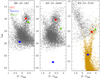 |
Fig. 8 Locations of the source, blend, and RGC centroid in the instrumental color-magnitude diagrams (CMDs) of the lensing events MOA-2022-BLG-563, KMT-2023-BLG-0469, and KMT-2023-BLG-0735. For KMT-2023-BLG-0735, the CMD is constructed by combining the KMTC data (gray dots) and HST (brown dots) data. |
Source parameters.
Angular source radius, Einstein radius, and relative lens-source proper motion.
5 Physical lens parameters
The physical parameters of the individual planetary systems were estimated from Bayesian analyses, which were conducted using the constraints given by the measured lensing observables. In the first step of the analysis, we produced a large number of artificial lensing events from a Monte Carlo simulation. For each simulated event, we assigned the mass M of the lens, which was derived from a model mass function, and the distances to the lens Dl and source DS, and their relative proper motion µ, which were derived from a Galaxy model. In the simulation, we adopted the Jung et al. (2018) model for the mass function, and the Jung et al. (2021) model for the Galaxy model. In the second step, we calculated the lensing observables of the event time scale and Einstein radius corresponding to the physical parameters (M, DL, DS, µ) of each simulated event from the relations
 (5)
(5)
where κ = 4G/(c2AU) ≃ 8.14 mas/M⊙, and πrel = πL – πS = AU(1/Dl – 1/DS) denotes the relative lens-source parallax. For all three events, the extra lensing observable of the microlens parallax πE could not be constrained, because either the event time scale was not long enough or the photometric precision of data was not high enough to detect the subtle deviations induced by the higher-order effects. In the third step, we constructed the posteriors of the lens mass and distance by imposing a weight to each event of
 (6)
(6)
where (tE, θE) denote the measured values of the lensing observables, and [σ(tE), σ(θE)] represent their uncertainties. Besides the lensing observables tE and θE, the blended flux can often provide a constraint on the lens system from the fact that the flux from the lens contributes to the blended light, and thus it should be less than the measured blended flux. We found that the blending constraint has little effects on the lens parameters, because the blended flux was high in all cases of the events.
We present the posterior distributions of the planet mass and distance to the planetary lens system for the individual events in Figs. 9 and 10, respectively. In each panel, the distributions drawn in blue and red represent the contributions by the disk and bulge lens populations, respectively, and the distribution drawn in black represents the sum of contributions by the two lens populations. In the panels of the planet-mass posteriors, we draw three dotted vertical lines corresponding to the masses of Jupiter (MJ), Uranus (MU), and Earth (ME) of the Solar System.
In Table 7, we list the physical parameters the host mass, Mh, planet mass, Mp, distance to the planetary system, DL, and the projected planet-host separation, a⊥. For the planetary separation, we present the values corresponding to the inner (a⊥,in) and outer (a⊥,out) solutions, and additionally present the value corresponding to the intermediate solution (a⊥,int) for KMT-2023-BLG-0469. For each lens parameter, the median of the Bayesian posterior distribution is chosen as the representative value, and the 16% and 84% of the posterior distribution are set as the upper and lower limits, respectively. Also presented are the snow line distances estimated as asnow ~ 2.7AU(M/M⊙) (Kennedy & Kenyon 2008), and the probabilities for the lenses to be in the disk, Pdisk, and bulge, Pbulge·
It is found that all three planets have masses lying between those of Jupiter and Uranus. For all planetary systems, the hosts of planets are main-sequence stars that are less massive than the Sun, and the planets lie well beyond the snow lines of the planetary systems. For the planet MOA-2022-BLG-563Lb, the estimated mass is 1.3 times of the mass of Saturn, and thus it is likely to be a giant planet. On the other hand, the masses of the planets KMT-2023-BLG-0469Lb and KMT-2023-BLG-0735Lb are approximately 2.7 times of the mass of Uranus, and thus they are more likely to be ice giants. In all cases, the planetary systems are more likely to be in the bulge with probabilities Pbulge = 64%, 73%, and 58% for MOA-2022-BLG-563, KMT-2023-BLG-0469, and KMT-2023-BLG-0735, respectively.
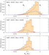 |
Fig. 9 Bayesian posteriors of the planet masses. The three dotted vertical lines represent the masses of Earth (ME), Uranus (MU), and Jupiter (MJ) of the Solar System. The curves drawn in red and blue indicate the contributions by the disk and bulge lens populations, respectively, and the black curve represents the sum of the contributions by the two lens populations. |
Physical lens parameters.
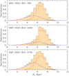 |
Fig. 10 Bayesian posteriors of the distances to the planetary systems. Notations are the same as those in Fig. 9. |
6 Summary and conclusion
We conducted analyses of the three microlensing events MOA-2022-BLG-563, KMT-2023-BLG-0469, and KMT-2023-BLG-0735, for which the lensing light curves exhibit short-term anomalies with dip features appearing near the peaks of the lensing light curves. From the detailed analyses of the anomalies, we found that the anomalies were produced by planets, for which the mass ratios between the planet and host are on the order of 10−4. All planetary systems share common properties that planets have masses lying between those of Jupiter and Uranus, the hosts of planets are main-sequence stars that are less massive than the Sun, and the planets lie beyond the snow lines of the planetary systems. We found that interpreting the anomalies was subject to a common inner-outer degeneracy, which causes ambiguity in estimating the projected planet-host separation, and identified an extra local solution resulting from an accidental degeneracy in the case of KMT-2023-BLG-0469.
Conducting morphological studies to classify lensing events based on similar anomalies and exploring the specific origins of each anomaly class is crucial. This not only aids in promptly diagnosing anomalies before in-depth analysis but also facilitates an accurate characterization of lens systems for future events sharing similar anomaly structures. The anomalies observed in the analyzed events share a distinctive trait, characterized by a brief dip surrounded by subtle bumps near the peak of the light curve. This particular feature strongly suggests a planetary origin for the anomaly.
Acknowledgements
Work by C.H. was supported by the grants of National Research Foundation of Korea (2019R1A2C2085965). This research has made use of the KMTNet system operated by the Korea Astronomy and Space Science Institute (KASI) at three host sites of CTIO in Chile, SAAO in South Africa, and SSO in Australia. Data transfer from the host site to KASI was supported by the Korea Research Environment Open NETwork (KREONET). This research was supported by the Korea Astronomy and Space Science Institute under the R&D program (Project No. 2023-1-832-03) supervised by the Ministry of Science and ICT. The MOA project is supported by JSPS KAKENHI Grant Nos. JP24253004, JP26247023, JP23340064, JP15H00781, JP16H06287, JP17H02871 and JP22H00153. J.C.Y., I.G.S., and SJ.C. acknowledge support from NSF Grant No. AST-2108414. Y.S. acknowledges support from NSF Grant No. 2020740. C.R. was supported by the Research fellowship of the Alexander von Humboldt Foundation.
References
- Adams, A. D., Boyajian, T. S., & von Braun, K., 2018, MNRAS, 473, 3608 [NASA ADS] [CrossRef] [Google Scholar]
- Albrow, M. 2017, https://doi.org/10.5281/zenodo.268049 [Google Scholar]
- Albrow, M., Beaulieu, J.-P., Birch, P., et al. 1998, ApJ, 509, 687 [NASA ADS] [CrossRef] [Google Scholar]
- Albrow, M., Horne, K., Bramich, D. M., et al. 2009, MNRAS, 397, 2099 [Google Scholar]
- Alcock, C., Akerlof, C. W., Allsman, R. A., et al. 1993, Nature, 365, 621 [NASA ADS] [CrossRef] [Google Scholar]
- An, J. H. 2005, MNRAS, 356, 1409 [Google Scholar]
- Aubourg, E., Bareyre, P., Bréhin, S., et al. 1993, Nature, 365, 623 [NASA ADS] [CrossRef] [Google Scholar]
- Bensby, T. Yee, J. C., Feltzing, S., et al. 2013, A&A, 549, A147 [NASA ADS] [CrossRef] [EDP Sciences] [Google Scholar]
- Bessell, M. S., & Brett, J. M. 1988, PASP, 100, 1134 [Google Scholar]
- Bond, I. A., Abe, F., Dodd, R. J., et al. 2001, MNRAS, 327, 868 [Google Scholar]
- Bond, I. A., Udalski, A., Jaroszynski, M., et al. 2004, ApJ, 606, L155 [NASA ADS] [CrossRef] [Google Scholar]
- Chung, S.-J., Han, C., Park, B.-G., et al. 2005, ApJ, 630, 535 [Google Scholar]
- Dominik, M. 1999, A&A, 349, 108 [NASA ADS] [Google Scholar]
- Doran, M., & Mueller, C. M. 2004, J. Cosmology Astropart. Phys., 09, 003 [CrossRef] [Google Scholar]
- Gaudi, B. S., & Gould, A. 1997, ApJ, 486, 85 [Google Scholar]
- Gonzalez, O. A., Rejkuba, M., Localize, M., et al. 2012, A&A, 543, A13 [NASA ADS] [CrossRef] [EDP Sciences] [Google Scholar]
- Gaudi, B. S. 1998, ApJ, 506, 533 [Google Scholar]
- Gould, A., & Loeb, L. 1992, ApJ, 396, 104 [NASA ADS] [CrossRef] [Google Scholar]
- Gould, A., Han, C., Weicheng, Z., et al. 2022, A&A, 664, A13 [NASA ADS] [CrossRef] [EDP Sciences] [Google Scholar]
- Griest, K., & Safizadeh, N. 1998, ApJ, 500, 37 [Google Scholar]
- Han, C. 2006, ApJ, 638, 1080 [Google Scholar]
- Han, C., & Gaudi, B. S. 2008, ApJ, 689, 53 [CrossRef] [Google Scholar]
- Han, C., Udalski, A., Gould, A., et al. 2017, AJ, 154, 133 [NASA ADS] [CrossRef] [Google Scholar]
- Han, C., Bond, I. A., Gould, A., et al. 2018, AJ, 156, 226 [Google Scholar]
- Han, C., Udalski, A., Kim, D., et al. 2021a, A&A, 650, A89 [NASA ADS] [CrossRef] [EDP Sciences] [Google Scholar]
- Han, C., Albrow, M. D., Chung, S.-J., et al. 2021b, A&A, 652, A145 [NASA ADS] [CrossRef] [EDP Sciences] [Google Scholar]
- Han, C., Udalski, A., Kim, D., et al. 2021c, A&A, 655, A21 [NASA ADS] [CrossRef] [EDP Sciences] [Google Scholar]
- Han, C., Gould, A., Kim, D., et al. 2022, A&A, 663, A145 [NASA ADS] [CrossRef] [EDP Sciences] [Google Scholar]
- Han, C., Lee, C.-U., Bond, I. A., et al. 2023, A&A, 676, A97 [NASA ADS] [CrossRef] [EDP Sciences] [Google Scholar]
- Holtzman, J. A., Watson, A. M., Baum, W. A., et al. 1998, AJ, 115, 1946 [Google Scholar]
- Hwang, K.-H., Zang, W., Gould, A., et al. 2022, AJ, 163, 43 [NASA ADS] [CrossRef] [Google Scholar]
- Jung, Y. K., Udalski, A., Gould, A., et al. 2018, AJ, 155, 219 [Google Scholar]
- Jung, Y. K., Han, C., Udalski, A., et al. 2021, AJ, 161, 293 [NASA ADS] [CrossRef] [Google Scholar]
- Jung, Y. K., Zang, W., Han, C., et al. 2022, AJ, 164, 262 [NASA ADS] [CrossRef] [Google Scholar]
- Kennedy, G. M., & Kenyon, S. J. 2008, ApJ, 673, 502 [Google Scholar]
- Kervella, P., Thévenin, F., Di Folco, E., & Ségransan, D. 2004, A&A, 426, 29 [Google Scholar]
- Kim, D.-J., Kim, H.-W., Hwang, K.-H., et al. 2018, AJ, 155, 76 [Google Scholar]
- Kim, S.-L., Lee, C.-U., Park, B.-G., et al. 2016, JKAS, 49, 37 [Google Scholar]
- Mayor, M., & Queloz, D. 1995, Nature, 378, 355 [Google Scholar]
- Mao, S., & Paczyński, B. 1991, ApJ, 374, 37 [Google Scholar]
- Minniti, D., Lucas, P. W., Emerson, J. P., et al. 2010, New Astron., 15, 433 [Google Scholar]
- Nataf, D. M., Gould, A., Fouqué, P., et al. 2013, ApJ, 769, 88 [Google Scholar]
- Udalski, A., Szymanski, M., Kałuzny, J., et al. 1994, Acta Astron., 44, 1 [NASA ADS] [Google Scholar]
- Wolszczan, A., & Frail, D. A. 1992, Nature, 355, 145 [CrossRef] [Google Scholar]
- Yee, J. C., Shvartzvald, Y., Gal-Yam, A., et al. 2012, ApJ, 755, 102 [Google Scholar]
- Yee, J. C., Zang, W., Udalski, A., et al. 2021, AJ, 162, 180 [NASA ADS] [CrossRef] [Google Scholar]
- Yoo, J., DePoy, D.L., Gal-Yam, A., et al. 2004, ApJ, 603, 139 [NASA ADS] [CrossRef] [Google Scholar]
All Tables
All Figures
|
Fig. 1 Light curve of MOA-2022-BLG-563. The top panel shows the whole view, and the lower panels show the zoom-in view around the anomaly and the residuals from the 2L1S and ILI S models. The solid and dashed curves drawn over the data points are the 2L1S and ILI S models, respectively. The colors of data points are set to match the labels of the observatories in the legend. |
| In the text | |
|
Fig. 2 ∆χ2 maps on the (log s, log q) parameter plane for the events MOA-2022-BLG-563 (top panel), KMT-2023-BLG-0469 (middle panel), and KMT-2023-BLG-0735 (bottom panel). Color coding is set to indicate points with ∆χ2 ≤ 12n (red), ≤22n (yellow), <32n (green), ≤42n (cyan), and ≤52n (blue), where n = 2. The dashed vertical line in each panel represents the geometric mean, (sin × sout)1/2, of the planet separations of the inner and outer solutions. |
| In the text | |
|
Fig. 3 Lens-system configurations of MOA-2022-BLG-563. The configurations of the inner and outer solutions are shown in the upper and lower panels, respectively. In each panel, the red figures represent the caustics, and the arrowed line is the source trajectory. Gray contours encompassing the caustics represent equi-magnification contours. The coordinates are centered at the center of mass of the planetary lens system, and the lengths are scaled to the Einstein radius. |
| In the text | |
|
Fig. 4 Light curve of KMT-2023-BLG-0469. The solid, dotted, and dashed curves on the data points represent the models of the outer, intermediate, and inner 2L1S solutions, respectively. |
| In the text | |
|
Fig. 5 Lens-system configurations of the inner (top panel), intermediate (middle panel), and outer (bottom panel) solutions for the lensing event KMT-2023-BLG-0469. Notations are same as those in Fig. 3. |
| In the text | |
|
Fig. 6 Light curve of KMT-2023-BLG-0735. |
| In the text | |
|
Fig. 7 Lens-system configurations of the inner (upper panel) and outer (lower panel) solutions for the lensing event KMT-2023-BLG-0735. Notations are same as those in Fig. 3. |
| In the text | |
|
Fig. 8 Locations of the source, blend, and RGC centroid in the instrumental color-magnitude diagrams (CMDs) of the lensing events MOA-2022-BLG-563, KMT-2023-BLG-0469, and KMT-2023-BLG-0735. For KMT-2023-BLG-0735, the CMD is constructed by combining the KMTC data (gray dots) and HST (brown dots) data. |
| In the text | |
|
Fig. 9 Bayesian posteriors of the planet masses. The three dotted vertical lines represent the masses of Earth (ME), Uranus (MU), and Jupiter (MJ) of the Solar System. The curves drawn in red and blue indicate the contributions by the disk and bulge lens populations, respectively, and the black curve represents the sum of the contributions by the two lens populations. |
| In the text | |
|
Fig. 10 Bayesian posteriors of the distances to the planetary systems. Notations are the same as those in Fig. 9. |
| In the text | |
Current usage metrics show cumulative count of Article Views (full-text article views including HTML views, PDF and ePub downloads, according to the available data) and Abstracts Views on Vision4Press platform.
Data correspond to usage on the plateform after 2015. The current usage metrics is available 48-96 hours after online publication and is updated daily on week days.
Initial download of the metrics may take a while.