| Issue |
A&A
Volume 689, September 2024
|
|
|---|---|---|
| Article Number | A209 | |
| Number of page(s) | 10 | |
| Section | Planets and planetary systems | |
| DOI | https://doi.org/10.1051/0004-6361/202450873 | |
| Published online | 13 September 2024 | |
KMT-2021-BLG-2609Lb and KMT-2022-BLG-0303Lb: Microlensing planets identified through signals produced by major-image perturbations
1
Department of Physics, Chungbuk National University,
Cheongju
28644,
Republic of Korea
2
University of Canterbury, Department of Physics and Astronomy,
Private Bag 4800,
Christchurch
8020,
New Zealand
3
Korea Astronomy and Space Science Institute,
Daejon
34055,
Republic of Korea
4
Max Planck Institute for Astronomy,
Königstuhl 17,
69117
Heidelberg,
Germany
5
Department of Astronomy, The Ohio State University,
140 W. 18th Ave.,
Columbus,
OH
43210,
USA
6
Department of Particle Physics and Astrophysics, Weizmann Institute of Science,
Rehovot
76100,
Israel
7
Center for Astrophysics | Harvard & Smithsonian
60 Garden St.,
Cambridge,
MA
02138,
USA
8
Department of Astronomy and Tsinghua Centre for Astrophysics, Tsinghua University,
Beijing
100084,
China
9
School of Space Research, Kyung Hee University, Yongin,
Kyeonggi
17104,
Republic of Korea
Received:
25
May
2024
Accepted:
19
July
2024
Abstract
Aims. We investigate microlensing data collected by the Korea Microlensing Telescope Network (KMTNet) survey during the 2021 and 2022 seasons to identify planetary lensing events displaying a consistent anomalous pattern. Our investigation reveals that the light curves of two lensing events, KMT-2021-BLG-2609 and KMT-2022-BLG-0303, exhibit a similar anomaly, in which short-term positive deviations appear on the sides of the low-magnification lensing light curves.
Methods. To unravel the nature of these anomalies, we meticulously analyze each of the lensing events. Our investigations reveal that these anomalies stem from a shared channel, wherein the source passed near the planetary caustic induced by a planet with projected separations from the host star exceeding the Einstein radius. We find that interpreting the anomaly of KMT-2021-BLG-2609 is complicated by the “inner–outer” degeneracy, whereas for KMT-2022-BLG-0303, there is no such issue despite similar lens-system configurations. In addition to this degeneracy, interpreting the anomaly in KMT-2021-BLG-2609 involves an additional degeneracy between a pair of solutions, in which the source partially envelops the caustic and the other three solutions in which the source fully envelopes the caustic. As in an earlier case of this so-called von Schlieffen–Cannae degeneracy, the former solutions have substantially higher mass ratio.
Results. Through Bayesian analyses conducted based on the measured lensing observables of the event time scale and angular Einstein radius, the host of KMT-2021-BLG-2609L is determined to be a low-mass star with a mass ~0.2 M⊙ in terms of a median posterior value, while the planet’s mass ranges from approximately 0.032 to 0.112 times that of Jupiter, depending on the solutions. For the planetary system KMT-2022-BLG-0303L, it features a planet with a mass of approximately 0.51 MJ and a host star with a mass of about 0.37 M⊙. In both cases, the lenses are most likely situated in the bulge.
Key words: planets and satellites: detection
Corresponding author; This email address is being protected from spambots. You need JavaScript enabled to view it.
© The Authors 2024
 Open Access article, published by EDP Sciences, under the terms of the Creative Commons Attribution License (https://creativecommons.org/licenses/by/4.0), which permits unrestricted use, distribution, and reproduction in any medium, provided the original work is properly cited.
This article is published in open access under the Subscribe to Open model. This email address is being protected from spambots. You need JavaScript enabled to view it. to support open access publication.
1 Introduction
Since the emergence of high-cadence surveys in the 2010s, there has been a significant increase in the detection of microlensing planets (Gould et al. 2022; Jung et al. 2022). According to the “NASA Exoplanet Archive1”, the number of known microlensing planets has risen to 223, making microlensing the third most productive method for planet discovery. Microlensing signals from planets occur when a source star passes close to a lensing caustic (Mao & Paczyński 1991; Gould & Loeb 1992). In gravitational microlensing, caustics are specific regions at which the magnification of a background point source becomes infinitely large due to the lensing effect. The characteristics of these caustics, including their position, size, and shape, depend on the separation of the planet from its host and their mass ratio (Chung et al. 2005; Han 2006). Additionally, the various trajectories of source stars relative to the lens system contribute to the diverse range of patterns observed in microlensing signals.
The increasing number of microlensing planets, along with the wide variety of signal forms, has led to a trend of jointly announcing discoveries that show similar anomaly patterns in their light curves. Han et al. (2017) and Poleski et al. (2017) provided notable examples of planetary signals arising from a recurring pathway in their analyses of the microlensing events OGLE-2016-BLG-0263 and MOA-2012-BLG-006, respectively. Han et al. (2024a) identified planetary signals characterized by brief dips flanked by shallow rises on either side in their analyses of three events: MOA-2022-BLG-563, KMT-2023-BLG-0469, and KMT-2023-BLG-0735. Weak short-term planetary signals generated without caustic crossings were exemplified by Han et al. (2023, 2021a) for the microlensing events KMT-2022-BLG-0475, KMT-2022-BLG-1480, KMT-2018-BLG-1976, KMT-2018-BLG-1996, and OGLE-2019-BLG-0954. Han et al. (2024b) announced the discoveries of three planets – KMT-2023-BLG-0416, KMT-2023-BLG-1454, and KMT-2023-BLG-1642 – identified from partially covered signals.
Recently, Han et al. (2024c) announced the discovery of four microlensing planets – KMT-2020-BLG-0757Lb, KMT-2022-BLG-0732Lb, KMT-2022-BLG-1787Lb, and KMT-2022-BLG-1852Lb – by analyzing signals observed on the wings of the lensing light curves. These signals originated from “minor-image” perturbations, occurring when source stars pass through peripheral caustics induced by “close” planets. In a separate study, Jung et al. (2021) identified planetary signals in the lensing events OGLE-2018-BLG-0567 and OGLE-2018-BLG-0962, for which the signals with positive deviations resulting from major-image perturbations appear on the sides of the light curves. Planets through signals of a similar type were reported from the analyses of the lensing events OGLE-2017-BLG-1777, OGLE-2017-BLG-0543 by Ryu et al. (2024) and OGLE-2017-BLG-0448 by Zhai et al. (2024). These perturbations occur when source stars traverse over peripheral caustics induced by “wide” planets. In the subsequent section, we explain the microlensing terminologies “close”, “wide”, “major image”, and “minor image”. This systematic classification of planetary signals facilitates the recognition of similar patterns within the light curves of upcoming lensing events.
In this study, we introduce two additional microlensing planets identified via signals produced through major-image perturbations: KMT-2021-BLG-2609Lb and KMT-2022-BLG-0303Lb. We discuss shared characteristics of the signals and explore the origins of these signals. Additionally, we offer detailed explanations of the typical types of degeneracies frequently encountered when interpreting planetary signals arising through this channel.
2 Signals through major-image perturbations
In the case where a single source undergoes microlensing by a single mass (referred to as a 1L1S event), the image of the source is split into two distinct images. One of these images, known as the “major image”, appears brighter and is located outside the Einstein ring, while the other, termed the “minor image”, appears fainter and is positioned inside the ring. Within the context of the lens plane, a planetary signal of a lens system comprising two masses (referred to as a 2L1S system) of a planet and its host emerges when the planet perturbs either of the source images. When the planet perturbs the major image, it induces further magnification of the image, resulting in positive anomalies in the lensing light curve. Conversely, when the minor image is perturbed by the planet, it experiences demagnification, leading to negative deviations. Given the positions of the two images, major-image perturbations occur when a planet has a separation greater than the Einstein radius (θE), while minorimage perturbations occur when the planet’s separation is less than the Einstein radius. In microlensing studies, lengths are typically scaled to θE, and the projected planet-host separation normalized to θE is represented as s (normalized separation). Consequently, the terms “close” and “wide” denote planets with s < 1 and s > 1, respectively.
The region of planetary perturbation in the lens plane corresponds to the position of caustics in the source plane. A planet induces two sets of caustics: one centered around the position of the planet’s host star (“central caustic”), and the other positioned away from the host (“planetary caustic”) at approximately
![Mathematical equation: $\[\mathbf{u}_{\mathrm{c}}=\mathrm{s}-\frac{1}{\mathrm{~s}}.\]$](/articles/aa/full_html/2024/09/aa50873-24/aa50873-24-eq1.png) (1)
(1)
Here s represents the position vector of the planet with respect to the host. If the mass ratio between a planet and its host star (q) is very low and the normalized separation is not precisely unity, then the central caustic induced by a wide planet with s and that induced by a close planet with 1/s display notable similarities (Dominik 1999; An 2005). However, the pair of planetary caustics induced by the close and wide planets differ from each other in number, shape, and location. A close planet results in a pair of three-fold caustics on the opposite side of the planet with respect to the host, while a wide planet produces a single fourfold caustic on the planet side. For both types of planets, the size of the planetary caustics decreases in proportion to the square root of the mass ratio between the planet and host (Han 2006). For a given planetary lens, the planetary caustic is substantially bigger than the central caustic. Figure 1 illustrates how the caustics vary depending on the planetary separation and mass ratio. Because of the positions of caustics, planetary signals resulting from central caustics appear near the peak of the light curve for high-magnification events (Griest & Safizadeh 1998), whereas signals caused by planetary caustics tend to emerge on the side of the light curve for events with low lensing magnifications.
3 Observations and data
The planetary lensing events analyzed in this study were identified by examining data collected from the Korea Microlensing Telescope Network (KMTNet: Kim et al. 2016) survey conducted during the 2021 and 2022 seasons. The KMTNet group operates a lensing experiment employing a network of three telescopes strategically located across the Southern Hemisphere: one at the Cerro Tololo Inter-American Observatory in Chile (KMTC), another at the South African Astronomical Observatory in South Africa (KMTS), and the third at the Siding Spring Observatory in Australia (KMTA). These telescopes are identical, each featuring a 1.6-meter aperture and equipped with a camera providing a field of view of 4 square degrees.
The microlensing survey involves monitoring star brightness in the Galactic bulge direction to detect gravitational lensing-induced light variations. The majority of star images were captured in the I band, with approximately one-tenth of images taken in the V band specifically for source color measurements. Data reduction and photometry employed the pipeline developed by Albrow et al. (2009), which incorporates the difference imaging analysis technique (Tomaney & Crotts 1996; Alard & Lupton 1998; Woźniak 2000). To ensure optimal data quality for our analysis, we performed a re-reduction of the KMTNet data using the photometry software developed by Yang et al. (2024). Error bars were adjusted not only to ensure consistency between the scatter of data and errors but also to establish χ2 per degree of freedom of unity for each data set. This process was carried out following the routine outlined in Yee et al. (2012).
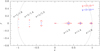 |
Fig. 1 Variation of lensing caustics induced by planets. We illustrate two sets of caustics with planet-to-host mass ratios q = 2 × 10⁻³ (depicted in red) and q = 2 × 10⁻⁴ (depicted in blue). Within each set, a series of caustics demonstrates variations depending on the planetary separation s. The coordinates are centered at the position of the planet host and the lengths are scaled to the Einstein radius. The dotted circle centered at the origin represents the Einstein ring. |
4 Analyses of anomalies
A planetary lens corresponds to a binary lens with a very low mass ratio between the lens components. In order to explain the observed anomalies in the lensing events, we conduct a 2L1S modeling. Assuming a rectilinear relative motion between the lens and source, the behavior of a 2L1S event is characterized by seven basic parameters. The first three parameters (t0, u0, tE) describe the source’s approach to the lens: t0 represents the time of the closest lens-source approach, u0 is the impact parameter of the approach, and tE denotes the event time scale. The 2L lens system is characterized by two additional parameters (s, q), where s denotes the projected separation (scaled to θE) and q represents the mass ratio between the lens components. The parameter α indicates the incidence angle of the source relative to the binary-lens axis. The last parameter, ρ, defined as the ratio of the angular source radius θ* scaled to θE, characterizes the deformation of the lensing light curve during planetary perturbations by finite-source effects (Bennett & Rhie 1996).
Through modeling, we determined the lensing solution comprising a set of parameters that best describe the observed anomalies. In this procedure, we searched for the binary parameters (s, q) using a grid approach with multiple initial values of α, while the remaining parameters were determined through a downhill approach using the Markov chain Monte Carlo (MCMC) algorithm. Throughout this process, we utilized the map-making method (Dong et al. 2006), an improved version of the ray-shooting method, to compute finite magnifications. Additionally, we examined the χ2 map on the grid parameter plane to assess the potential existence of degenerate solutions. In the concluding phase, we fine-tuned the parameters of the identified local solution, allowing for variability.
It is known that planetary signals arising from major-image perturbations can often be mimicked by a subset of binary-source (1L2S) events with extreme flux ratios between the source stars (Gaudi 1998; Gaudi & Han 2004). To assess the degeneracy between 2L1S and 1L2S interpretations for each event, we conduct additional modeling under the 1L2S scenario. Modeling a 1L2S event requires incorporating three additional parameters (t0,2, u0,2, qF) alongside the parameters (t0, u0, tE) of a 1L1S model, to address the anomalies resulting from the presence of a companion (S2) to the primary source (S1) (Hwang et al. 2013). Here, (t0,2, u0,2) designate the closest approach time and impact parameter of S2, while qF represents the flux ratio between the companion and primary source stars. In cases for which the lens passes over either of the source stars, additional parameters ρ1 and/or ρ2 should be included in the modeling. In the 1L2S modeling process, we initially determine the parameters of the 1L1S solution by analyzing the data while excluding those in the region around the anomaly. Subsequently, we ascertain the binary-source parameters, taking into account the location and magnitude of the anomaly. In the following subsections, we present the analyses of the individual events.
4.1 KMT-2021-BLG-2609
The lensing event KMT-2021-BLG-2609 was found through the KMTNet survey during the later stage of the bulge season on September 24, 2021, corresponding to the reduced Heliocentric Julian date HJD′ = HJD – 2450000 = 9481. The equatorial coordinates of the source are (RA, Dec)J2000 = (17:34:04.53, −27:35:48.98), which corresponds to the Galactic coordinates (l, b) = (−0°.2160, −2°.8649). The source has a baseline magnitude Ibase = 18.48 and the I-band extinction toward the field is AI = 3.29. The extinction is estimated as AI = 7 AK, where the K-band extinction AK was adopted from Gonzalez et al. (2012). The source lies in the BLG15 field toward which observations were conducted with a 1-hour cadence.
Figure 2 displays the light curve of the lensing event KMT-2021-BLG-2609. Notably, there are no data points available after HJD′ ~ 9507, marking the conclusion of the bulge season. The event reached its peak magnification on HJD′ ~ 9497.9, exhibiting a relatively low magnification of Apeak ~ 1.6. Approximately four days before reaching its peak, the light curve exhibited a positive anomaly lasting for about two days. The upper panel of Figure 2 provides a zoomed-in view of this anomaly region, which was captured by data obtained from all three KMTNet telescopes.
Two scenarios can explain a short-term positive anomaly in the light curve of a low-magnification event. The first scenario involves a planetary interpretation, in which the signal arises from the source nearing a planetary caustic positioned away from the location of the planet’s host. The second scenario entails a 1L2S interpretation, in which the main light curve is generated by the primary source’s approach to the lens with a large impact parameter, while the anomaly results from the close approach of a very faint companion source to the lens. We investigate both scenarios.
From the modeling conducted under the planetary lens scenario, we have identified five distinct local solutions. In Figure 3, the positions of these individual solutions are depicted on the Δξ-log q parameter plane, where Δξ = u0/ sin α − (s − 1/s) represents the separation between the source and the center of the planetary caustic at the time of the planetary perturbation (Hwang et al. 2018). Among these solutions, three exhibit smaller mass ratios falling within the range of q ~ (0.15–0.22) × 10−3, while the remaining two solutions feature larger mass ratios q ~ (0.53–0.58) × 10−3. We designate the former and latter solution groups as “small q” and “large q” solutions, respectively.
Further investigation reveals that the two solutions within the “large-q” group, with Δξ ~ 0.04 and +0.04, originate from the inner–outer degeneracy initially identified by Gaudi & Gould (1997). These solutions are hence labeled as “large q inner” and “large q outer” solutions. Similarly, the two solutions in the “small-q” group with Δξ ~ 0.02 and +0.02 also arise from this degeneracy, while the other solution has a separation Δξ ~ 0.0. We designate these solutions as “small q inner”, “small q outer”, and “small q intermediate” solutions. The degeneracy between the intermediate and the other solutions was extensively analyzed by Hwang et al. (2018). They termed the solution as “Cannae” for a scenario in which the source entirely encompasses the planetary caustic, while they labeled the solution as “von Schlieffen” for a situation in which the source encompasses only one flank of the caustic. According to this classification, the two large-q solutions are von Schlieffen solutions, while all three of the remaining solutions, that is, small-q solutions, are Cannae solutions. We note that, exactly as was the case for OGLE-2017-BLG-0173 (Hwang et al. 2018), the von Schlieffen solutions have substantially higher mass ratios than the Cannae solutions. We conjecture that this is a generic feature of the Cannae–von Schlieffen degeneracy, but we do not further pursue this question here.
In Table 1, we present the lensing parameters for the solutions obtained under the 2L1S scenario, along with the corresponding χ2 values for the fits. Figure 4 illustrates the model curves for the five solutions and residuals from the models in the vicinity of the anomaly. It is observed that the degeneracy among the solutions is highly pronounced, with χ2 differences among them being Δχ2 ≤ 1.4.
Figure 5 illustrates the lens-system configurations of the individual local solutions. The top panel presents a broader view, including the planetary caustic and the position of the planet, while the lower panels depict a zoomed-in perspective around the caustic for the individual local solutions. In all examined cases, the anomaly was interpreted through the source approach to the planetary caustic induced by a planet for which the projected planetary separation exceeded unity. According to the inner solution, the source traversed the inner region of the planetary caustic relative to the planet’s host, whereas according to the outer solution, it traversed the outer region. For the small-q intermediate solution, the source center passed very close to the caustic center. In all instances, the source passed over the caustic, leading to the determination of the normalized source radius. Notably, all solutions yield similar normalized source radii falling within the range of ρ ~ (29.8–34.8) × 10−3 in terms of a median value.
It is known that the planetary separations of the pair of solutions subject to the inner–outer degeneracy follow the relationship established by Hwang et al. (2022) and Gould et al. (2022):
![Mathematical equation: $\[s_{ \pm}^{\dagger}=\sqrt{s_{\text {inner }} \times s_{\text {outer }}}=\frac{\sqrt{u_{\mathrm{anom}}^2+4} \pm u_{\mathrm{anom}}}{2}.\]$](/articles/aa/full_html/2024/09/aa50873-24/aa50873-24-eq2.png) (2)
(2)
Here uanom represents the lens-source separation at the time of the anomaly (tanom), given by:
![Mathematical equation: $\[u_{\text {anom }}=\sqrt{u_0^2+\tau_{\text {anom }}^2} ; \qquad \tau_{\text {anom }}=\frac{t_{\text {anom }}-t_0}{t_{\mathrm{E}}}.\]$](/articles/aa/full_html/2024/09/aa50873-24/aa50873-24-eq3.png) (3)
(3)
The symbols “+” and “−” in the first and last terms of Eq. (2) indicate the perturbations corresponding to the major and minor images, respectively. For the pair of inner and outer solutions in the small q group with (t0, u0, tE, tanom) ~ (9498.0, 0.78, 16.0, 9493.5)2, we find that ![Mathematical equation: $\[s_{+}^{\dagger}=1.497\]$](/articles/aa/full_html/2024/09/aa50873-24/aa50873-24-eq4.png) , closely aligning with the geometric mean of the planetary separations, (sinner × souter)1/2 ~ 1.492. Similarly, for the pair of inner and outer solutions in the large q group with (t0, u0, tE, tanom) ~ (9497.9, 0.67, 17.4, 9493.5), we determine that
, closely aligning with the geometric mean of the planetary separations, (sinner × souter)1/2 ~ 1.492. Similarly, for the pair of inner and outer solutions in the large q group with (t0, u0, tE, tanom) ~ (9497.9, 0.67, 17.4, 9493.5), we determine that ![Mathematical equation: $\[s_{+}^{\dagger}=1.420\]$](/articles/aa/full_html/2024/09/aa50873-24/aa50873-24-eq5.png) , which again closely aligns with the geometric mean of the planetary separations, (sinner × souter)1/2 ~ 1.423. The fact that the lensing parameters of the two solutions conform to the analytic relation derived from investigating the lensing properties of the inner and outer solutions suggests that the pair of solutions arises from the inner–outer degeneracy.
, which again closely aligns with the geometric mean of the planetary separations, (sinner × souter)1/2 ~ 1.423. The fact that the lensing parameters of the two solutions conform to the analytic relation derived from investigating the lensing properties of the inner and outer solutions suggests that the pair of solutions arises from the inner–outer degeneracy.
We find that the 1L2S model is less favored for two major reasons, even though it approximately delineates the anomaly. Firstly, the 1L2S model provides a worse fit compared to the planetary solution, with a Δχ2 ~ 23. The lensing parameters for the 1L2S solution are provided in Table 2, and the model curve and residual are depicted in Figure 4. Notably, the 1L2S model fails to accurately describe the slight negative deviations just before and after the main bump of the anomaly, which are well-captured by the planetary model. Secondly, the 1L2S parameters are physically implausible. In Section 5, we will show that the de-reddened magnitude of the primary source for the 1L2S solution is ![Mathematical equation: $\[I_{S_1, 0}=14.40\]$](/articles/aa/full_html/2024/09/aa50873-24/aa50873-24-eq6.png) , that is, similar to the 2L1S solution. Therefore, the magnitude of the secondary source is
, that is, similar to the 2L1S solution. Therefore, the magnitude of the secondary source is ![Mathematical equation: $\[I_{S_{2,0}}=I_{S_1, 0}-2.5 ~\log \left(q_F\right)=21.3\]$](/articles/aa/full_html/2024/09/aa50873-24/aa50873-24-eq7.png) , which corresponds to an early M dwarf with a physical radius R2 ≃ 0.5 M⊙, which corresponds to an angular radius θ*,2 ≃ 0.3 μas. These numbers imply θE ≃ 15 μas, and so a relative lens-source proper motion μ ≃ 0.4 mas/yr. According to Equations. (22) and (23) of Gould (2022), the probability of such a low proper motion (for events consistent with a planetary interpretation) is p = (μ/6 mas yr−1) ~ 0.0045. Combined with the fact that this solution is also disfavored by Δχ2 = 23.4, this low p-value implies that this solution is effectively ruled out. However, because ρ2 is relatively weakly constrained, due diligence requires that we consider the possibility that ρ2 is much smaller than the best fit value given in Table 2, which would eliminate the low-proper-motion argument. Therefore, in the final column of Table 2, we report results for a 1L2S solution with ρ2 fixed at ρ2 = 0. Table 2 shows that such a solution has yet higher χ2, that is, Δχ2 = 37.6, showing that such solutions are also ruled out. We therefore find that this event is securely 2L1S. Given that the 2L1S model adequately explains the observed anomaly, we do not consider more complex models such as the binary-lens binary-source (2L2S) model, as illustrated by the planetary event KMT-2021-BLG-1898 (Han et al. 2022), or the triple-lens (3L1S) model, as illustrated by the planetary event OGLE-2023-BLG-0836 (Han et al. 2024c).
, which corresponds to an early M dwarf with a physical radius R2 ≃ 0.5 M⊙, which corresponds to an angular radius θ*,2 ≃ 0.3 μas. These numbers imply θE ≃ 15 μas, and so a relative lens-source proper motion μ ≃ 0.4 mas/yr. According to Equations. (22) and (23) of Gould (2022), the probability of such a low proper motion (for events consistent with a planetary interpretation) is p = (μ/6 mas yr−1) ~ 0.0045. Combined with the fact that this solution is also disfavored by Δχ2 = 23.4, this low p-value implies that this solution is effectively ruled out. However, because ρ2 is relatively weakly constrained, due diligence requires that we consider the possibility that ρ2 is much smaller than the best fit value given in Table 2, which would eliminate the low-proper-motion argument. Therefore, in the final column of Table 2, we report results for a 1L2S solution with ρ2 fixed at ρ2 = 0. Table 2 shows that such a solution has yet higher χ2, that is, Δχ2 = 37.6, showing that such solutions are also ruled out. We therefore find that this event is securely 2L1S. Given that the 2L1S model adequately explains the observed anomaly, we do not consider more complex models such as the binary-lens binary-source (2L2S) model, as illustrated by the planetary event KMT-2021-BLG-1898 (Han et al. 2022), or the triple-lens (3L1S) model, as illustrated by the planetary event OGLE-2023-BLG-0836 (Han et al. 2024c).
2L1S lensing parameters of KMT-2021-BLG-2609.
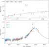 |
Fig. 2 Light curve of the lensing event KMT-2021-BLG-2609. The lower panel shows the entire view, while the upper panel provides a close-up of the anomaly region. The colors of the data points match those in the legend, representing the telescopes employed for data acquisition. The solid curve drawn over the data points is a 1L1S model obtained by excluding the data around the anomaly. |
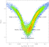 |
Fig. 3 Scatter plot of points in the MCMC chain for the 2L1S model of KMT-2021-BLG-2609. The ellipses mark the approximate locations of the five local solutions. The color codeing is set to represent points with ≤1σ (red), ≤2σ (yellow), ≤3σ (green), σ4σ (cyan), and ≤5σr (blue). |
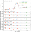 |
Fig. 4 Zoomed-in view around the anomaly region of KMT-2021-BLG-2609. The data points are overlaid with the model curves representing the intermediate, inner, and outer 2L1S solutions, as well as the 1L1S and 1L2S solutions. The residuals from the individual models are displayed in the lower panels. |
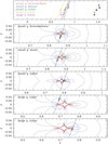 |
Fig. 5 Lens-system configurations of the lensing event KMT-2021-BLG-2609 for the five local solutions. The top panel provides a wide-angle perspective, showcasing the caustic and the position of the planet. The planet is marked by a small filled dot. Each of the lower panels presents a close-up view around the caustic. In these panels, the red figure indicates the caustic, while the arrowed line represents the source trajectory. The grey curves surrounding the caustic represent equi-magnification contours. Additionally, the blue circle positioned on the source trajectory represents the source whose size is adjusted to match that of the caustic. |
1L2S lensing parameters of KMT-2021-BLG-2609.
4.2 KMT-2022-BLG-0303
The microlensing event KMT-2022-BLG-0303 was first identified on April 4, 2022, corresponding to HJD′ ~ 9673. The equatorial and Galactic coordinates of the source are (RA, Dec)J2000 = (17:52:07.95, −22:41:20.69) and (l,b) = (+6°.1105,-1°.9615), respectively. The I-band baseline magnitude of the source is Ibase = 16.48 and the extinction toward the field is AI = 1.64. The source lies in the BLG38 field and observations were done with a 2.5-hour cadence.
The event reached its maximum magnification at around HJD′ ~ 9689.2, with a relatively low magnification of Apeak ~ 1.7. Figure 6 illustrates the light curve of the event, revealing a prominent anomaly appearing in the falling side of the light curve centered around HJD′ ~ 9713. The anomaly was covered through the integration of the KMTC and KMTS datasets, revealing a distinctive dual bump pattern: a prominent peak centered around HJD′ ~ 9712.3 and a secondary peak around HJD′ ~ 9714.2
From the 2L1S modeling, we identified a pair of local planetary solutions with (s, q)inner ~ (1.61, 1.33 × 10⁻³) and (s, q)outer ~ (1.60, 0.58 × 10⁻³). These solutions arise from the inner–outer degeneracy. The complete lensing parameters for both solutions are presented in Table 3, and the model curves around the region of the anomaly are depicted in Figure 7. Unlike the previous event KMT-2021-BLG-2609, the degeneracy in KMT-2022-BLG-0303 is significantly less severe, and the inner solution is strongly favored over the outer solution, with a substantial χ2 difference of Δχ2 = 79.2.
The reason for resolving the degeneracy became apparent upon scrutinizing the configuration of the lens system illustrated in Figure 8. Similar to the case of KMT-2021-BLG-2609, the configuration suggests that the anomaly originated from the close approach of the source to the planetary caustic, induced by the presence of the wide planet. While the caustic configurations resemble those of KMT-2021-BLG-2609, there is an important difference: the ratio of the source size to the caustic size for KMT-2022-BLG-0303 is substantially smaller than that for KMT-2021-BLG-2609. As a result, the anomaly reflects the structure of the caustic, leading to the observed dual-bump feature: the strong bump occurs when the source approaches the strong on-axis cusp of the caustic, while the weak bump arises when the source nears the weak off-axis cusp. In contrast, the outer solution fails to generate this dual-bump feature because the source initially approaches the off-axis cusp. Because the source encompasses one flank of the caustic, the normalized source radius was constrained to be ρ = (16.75 ± 0.51) × 10−3. The dual nature of the anomaly also facilitates the resolution of the degeneracy between the planetary and 1L2S interpretations, and it was found that the inner 2L1S model is favored over the 1L2S model by Δχ2 = 435.4.
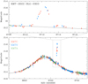 |
Fig. 6 Lensing light curve of KMT-2022-BLG-0303. The notations used are same as those presented in Fig. 2. |
Lensing parameters of KMT-2022-BLG-0303.
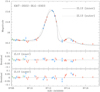 |
Fig. 7 Zoomed-in view around the anomaly region of KMT-2022-BLG-0303. The model curves of the inner and outer 2L1S solutions and their residuals are presented. |
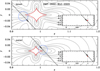 |
Fig. 8 Configurations of KMT-2022-BLG-0303 lens system. The notations correspond to those utilized in Fig. 5. |
5 Source stars and angular Einstein radii
In this section, we provide detailed specifications regarding the source stars involved in the events. Identifying source stars is crucial not only for fully characterizing the events but also for determining the angular Einstein radius. The Einstein radius is computed using the relation
![Mathematical equation: $\[\theta_{\mathrm{E}}=\frac{\theta_*}{\rho},\]$](/articles/aa/full_html/2024/09/aa50873-24/aa50873-24-eq8.png) (4)
(4)
where the angular source radius θ* can be deduced from the source type and the normalized source radius is measured from modeling.
We defined the type of the source by measuring its reddening and extinction-corrected (de-reddened) color (V − I)S,0 and brightness Is,0. In the initial phase of this procedure, we estimated the instrumental color and magnitude (V − I, I)S by conducting regression analysis on the data sets obtained from the pyDIA photometry code for both the V-band and I-band, relative to the model. Figure 9 shows the locations of the source stars for the individual events on the color-magnitude diagrams (CMDs) of stars lying near the source stars. For both events, obtaining reliable V-band source magnitude posed challenges because of either poor data quality or sparse coverage during the lensing magnification phase. In this case, we determined the source color by averaging the colors of stars positioned on either the giant or main-sequence branches of the combined CMD, with I-band magnitude offsets from the centroid red giant clump (RGC) falling within the measured value’s range. The CMD was compiled by merging CMDs obtained from KMTC and Hubble Space Telescope (HST) observations. The HST CMD data were derived from star observations in Baade’s Window conducted by Holtzman et al. (1998), and alignment of the KMTC and HST CMDs was achieved by utilizing the centroids of the RGC in the respective CMDs.
In the second phase, we calibrated the source color and magnitude. This calibration was performed using the approach introduced by Yoo et al. (2004). In this methodology, the RGC centroid served as a calibration reference because of its well-established de-reddened color and magnitude. By measuring the offsets of the source in color and magnitude from the RGC centroid, denoted as Δ(V − I, I)S, we calculated the de-reddened color and magnitude of the source as
![Mathematical equation: $\[(V-I, I)_{\mathrm{S}, 0}=(V-I, I)_{\mathrm{RGC}, 0}+\Delta(V-I, I)_{\mathrm{S}}.\]$](/articles/aa/full_html/2024/09/aa50873-24/aa50873-24-eq9.png) (5)
(5)
Here, (V − I, I)rgC,0 represents the de-reddened color and magnitude of the RGC centroid. We adopted the (V − I)rgC,0 value from Bensby et al. (2013) and the IrgC,0 value from Nataf et al. (2013). In Table 4, we list the values of (V − I, I)s, (V − I, I)rgc, (V − I, I)rgC,0, and (V − I, I)S,0, for the analyzed events. Upon analyzing the determined colors and magnitudes, it was observed that the source stars in both events are K-type giants.
In the third phase, we derived the angular source radius from the measured source color and magnitude, and then estimated angular Einstein radius. To derive θ*, we initially transformed the V − I color into V − K color using the Bessell & Brett (1988) relation. Next, we determined θ* based on the Kervella et al. (2004) relationship between the (V − K, I) and the angular stellar radius. With the estimated source radius, the angular Einstein radius was measured using the relation in Eq. (4), and the relative lens-source proper motion was calculated as
![Mathematical equation: $\[\mu=\frac{\theta_{\mathrm{E}}}{t_{\mathrm{E}}}.\]$](/articles/aa/full_html/2024/09/aa50873-24/aa50873-24-eq10.png) (6)
(6)
In Table 5, we list the estimated values of the angular source radius, Einstein radius, and relative proper motion for the individual events. For KMT-2021-BLG-2609, we computed estimates for θE and μ based on the ρ and tE values obtained from the small-q intermediate solution, which provides the best fit to the data. Notably, the alternative solutions yield tE and ρ values that are comparable, resulting in θE and μ estimates similar to the presented values.
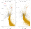 |
Fig. 9 Source locations in the instrumental color-magnitude diagrams with respect to the centroids of red giant clump (RGC). In each panel, grey and brown dots represent CMDs derived from KMTC and HST observations, respectively. |
Source parameters and spectral types.
Einstein radii and relative lens-source proper motions.
6 Physical parameters of planetary systems
In this section, we estimate the masses of the planet and host, along with the distance for each individual planetary system. The physical parameters were determined based on the lensing observables, including the event time scale and the angular Einstein radius. These observables are related to the mass M and distance DL by the relations
![Mathematical equation: $\[t_{\mathrm{E}}=\frac{\theta_{\mathrm{E}}}{\mu} ; \quad \theta_{\mathrm{E}}=\left(\kappa M \pi_{\mathrm{rel}}\right)^{1 / 2},\]$](/articles/aa/full_html/2024/09/aa50873-24/aa50873-24-eq11.png) (7)
(7)
where κ = 4G/(c2AU) ≃ 8.14 mas/M⊙, πrel = πL − πS = AU(1/DL − 1/Ds) represents the relative lens-source parallax, and DS denotes the distance to the source. Besides these observables, the physical lens parameters can be more precisely determined by measuring an additional observable of the micro-lens parallax πE, with which the mass and distance can be uniquely determined using the Gould (2000) relations:
![Mathematical equation: $\[M=\frac{\theta_{\mathrm{E}}}{\kappa \pi_{\mathrm{E}}} ; \quad D_{\mathrm{L}}=\frac{\mathrm{AU}}{\pi_{\mathrm{E}} \theta_{\mathrm{E}}+\pi_{\mathrm{S}}}.\]$](/articles/aa/full_html/2024/09/aa50873-24/aa50873-24-eq12.png) (8)
(8)
For none of the events could the microlens parallax be measured, either because of the relatively short time scales or because of the incomplete light curve coverage.
To estimate the mass and the distance to the lens, we conducted Bayesian analyses. These analyses integrated priors derived from the physical and dynamical distribution, as well as the mass function of lens objects, along with the constraints provided by tE and θE. In the analysis, we initially generated a large number of artificial lensing events using a Monte Carlo simulation. In the simulations, we allocated the locations of the lens and source, as well as their relative proper motion, based on a Galactic model. The mass of the lens was assigned using a mass function model. Specifically, we utilized the Galactic model proposed by Jung et al. (2021) and the mass-function model introduced by Jung et al. (2018). Using the provided values of (M, DL, DS,μ), we then calculated the lensing observables (tE,i, θE,i) for each artificial event by applying the relations given in Eq. (7). Finally, we obtained posteriors of M and DL by constructing their weighted distributions of simulated events. The weight assigned to each event was computed as
![Mathematical equation: $\[w_i=\exp \left(-\frac{\chi_i^2}{2}\right) ; \quad \chi_i^2=\left[\frac{t_{\mathrm{E}, i}-t_{\mathrm{E}}}{\sigma\left(t_{\mathrm{E}}\right)}\right]^2+\left[\frac{\theta_{\mathrm{E}, i}-\theta_{\mathrm{E}}}{\sigma\left(\theta_{\mathrm{E}}\right)}\right]^2,\]$](/articles/aa/full_html/2024/09/aa50873-24/aa50873-24-eq13.png) (9)
(9)
where [tE ± σ(tE), θE ± σ(θE)] denote the measured values and uncertainties for the lensing observables.
Figures 10 and 11 illustrate the posterior distributions of mass and distance for the planetary systems. Within each distribution, we indicate the median value using a vertical solid line, while the uncertainty range is delineated by two dotted lines. Table 6 provides a summary of parameters including host mass (Mhost), planet mass (Mplanet), distances to the lens (DL) and source (DS), and projected planet-host separation (a⊥). The source distances were also derived from the Bayesian analyses based on the Galatic model. For each parameter, the upper and lower limits are defined as the 16th and 84th percentiles of the Bayesian posterior. The projected separation was estimated from the relation a⊥ = sθEDL. For KMT-2021-BLG-2609L, we present two values of the planet mass corresponding to the small and large q solutions.
For the planetary system KMT-2021-BLG-2609L, the host is identified as a low-mass star with a mass of ~0.20 M⊙. The planet’s mass varies depending on the solution: it is ~0.032 MJ according to the small q solution and ~0.112 MJ according to the large q solution. For the system KMT-2022-BLG-0303L, it features a planet with a mass ~0.51 MJ and a host star with a mass ~0.37 M⊙. The estimated distances are ~7.5 kpc for KMT-2021-BLG-2609L and ~6.6 kpc for KMT-2022-BLG-0303L. Table 6 presents the probabilities for the lens to be located in the disk (pdisk) and bulge (pbulge). For both events, the probability of the lens being situated in the bulge exceeds 70%.
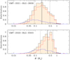 |
Fig. 10 Bayesian posteriors for the masses of the planetary systems’ host stars. Within each panel, the blue and red curves represent the contributions from the disk and bulge lens populations, respectively. The combined contribution of both populations is depicted by the black curve. The solid vertical line indicates the median value for each distribution, while the two dotted vertical lines denote the 1σ uncertainty range. |
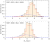 |
Fig. 11 Bayesian posteriors for the distances to the planetary systems. The notation system employed here is consistent with that of Fig. 10. |
7 Summary and conclusion
We analyzed the two microlensing events KMT-2021-BLG-2609 and KMT-2022-BLG-0303. The light curves of these events exhibited anomalies with similar traits: short-term positive signals appearing on the sides of the lensing light curves of low-magnification events. Through detailed examination of each event, we found that these anomalies originated from a common channel, wherein the source passed near the planetary caustic induced by a planet with projected separations from the host star exceeding the Einstein radius.
We conducted a thorough examination of the typical degeneracies often encountered in interpreting planetary signals arising from this channel. Our investigation uncovered that interpreting the anomaly of KMT-2021-BLG-2609 was affected by the well-known “inner–outer” degeneracy. In contrast, despite sharing a similar lens-system configuration, interpreting the anomaly of KMT-2022-BLG-0303 did not face this degeneracy. This was attributed to the substantially smaller ratio of the source size to the caustic size for KMT-2022-BLG-0303 than that for KMT-2021-BLG-2609. In addition to the inner–outer degeneracy, interpreting the anomaly in KMT-2021-BLG-2609 is subject to an additional degeneracy between Cannae and von Schlieffen solutions. In the Cannae solution, the source entirely encompasses the caustic, while in the von Schlieffen solution, the source only partially encompasses the caustic. Furthermore, we found that the mass ratios of the two von Schlieffen solutions were systematically higher than those of the three Cannae solutions. Noting that this was similar to the situation for OGLE-2017-BLG-0173 (Hwang et al. 2018), we conjectured that this is a generic feature of the Cannae–von Schlieffen degeneracy.
We utilized Bayesian analyses to estimate the physical parameters of the planetary systems, leveraging the constraints provided by the measured observables of the events. From this analysis, the host of KMT-2021-BLG-2609L is determined to be a low-mass star with a mass approximately 0.2 times that of the Sun, while the planet’s mass ranges from approximately 0.032 to 0.112 times that of Jupiter, depending on the solutions. For the planetary system KMT-2022-BLG-0303L, it includes a planet with a mass roughly half that of Jupiter and a host star with a mass approximately 0.37 times that of the Sun. It is notable that in both lensing events, the lenses are likely positioned in the bulge.
Physical lens parameters.
Acknowledgements
Work by C.H. was supported by the grant of National Research Foundation of Korea. This research has made use of the KMTNet system operated by the Korea Astronomy and Space Science Institute (KASI) at three host sites of CTIO in Chile, SAAO in South Africa, and SSO in Australia. Data transfer from the host site to KASI was supported by the Korea Research Environment Open NETwork (KREONET). This research was supported by KASI under the R&D program (Project No. 2024-1-832-01) supervised by the Ministry of Science and ICT. W.Z. acknowledges the support from the Harvard-Smithsonian Center for Astrophysics through the CfA Fellowship. J.C.Y., I.G.S., and S.J.C. acknowledge support from NSF Grant No. AST-2108414. Y.S. acknowledges support from NSF Grant No. 2020740.
References
- Alard, C., & Lupton, R. H. 1998, ApJ, 503, 325 [Google Scholar]
- Albrow, M., Horne, K., Bramich, D. M., et al. 2009, MNRAS, 397, 2099 [Google Scholar]
- An, J. H. 2005, MNRAS, 356, 1409 [Google Scholar]
- Bennett, D. P., & Rhie, S. H. 1996, ApJ, 472, 660 [NASA ADS] [CrossRef] [Google Scholar]
- Bensby, T. Yee, J. C., Feltzing, S., et al. 2013, A&A, 549, A147 [NASA ADS] [CrossRef] [EDP Sciences] [Google Scholar]
- Bessell, M. S., & Brett, J. M. 1988, PASP, 100, 1134 [Google Scholar]
- Chung, S.-J., Han, C., Park, B.-G., et al. 2005, ApJ, 630, 535 [Google Scholar]
- Dominik, M. 1999, A&A, 349, 108 [NASA ADS] [Google Scholar]
- Dong, Subo, DePoy, D. L., Gaudi, B. S., et al. 2006, ApJ, 642, 842 [NASA ADS] [CrossRef] [Google Scholar]
- Gaudi, B. S. 1998, ApJ, 506, 533 [Google Scholar]
- Gaudi, B. S., & Gould, A. 1997, ApJ, 486, 85 [Google Scholar]
- Gaudi, B. S., & Han, C. 2004, ApJ, 611, 528 [NASA ADS] [CrossRef] [Google Scholar]
- Gonzalez, O. A., Rejkuba, M., Localize, M., et al. 2012, A&A, 543, A13 [NASA ADS] [CrossRef] [EDP Sciences] [Google Scholar]
- Gould, A. 2000, ApJ, 542, 785 [NASA ADS] [CrossRef] [Google Scholar]
- Gould, A. 2022, arXiv e-prints [arXiv:2209.12501] [Google Scholar]
- Gould, A., & Loeb, L. 1992, ApJ, 396, 104 [NASA ADS] [CrossRef] [Google Scholar]
- Gould, A., Han, C., Weicheng, Z., et al. 2022, A&A, 664, A13 [NASA ADS] [CrossRef] [EDP Sciences] [Google Scholar]
- Griest, K., & Safizadeh, N. 1998, ApJ, 500, 37 [Google Scholar]
- Han, C. 2006, ApJ, 638, 1080 [Google Scholar]
- Han, C., Udalski, A., Gould, A., et al. 2017, AJ, 154, 133 [NASA ADS] [CrossRef] [Google Scholar]
- Han, C., Udalski, A., Kim, D., et al. 2021, A&A, 650, A89 [NASA ADS] [CrossRef] [EDP Sciences] [Google Scholar]
- Han, C., Gould, A., Kim, D., et al. 2022, A&A, 663, A145 [NASA ADS] [CrossRef] [EDP Sciences] [Google Scholar]
- Han, C., Udalski, A., Jung, Y. K., et al. 2023, A&A, 670, A172 [NASA ADS] [CrossRef] [EDP Sciences] [Google Scholar]
- Han, C., Jung, Y. K., Bond, I. A., et al. 2024a, A&A, 683, A115 [NASA ADS] [CrossRef] [EDP Sciences] [Google Scholar]
- Han, C., Udalski, A., Lee, C.-U., et al. 2024b, A&A, 6, A187 [NASA ADS] [CrossRef] [EDP Sciences] [Google Scholar]
- Han, C., Bond, I. A., Lee, C.-U., et al. 2024c, A&A, 687, A225 [NASA ADS] [CrossRef] [EDP Sciences] [Google Scholar]
- Han, C., Udalski, A., Jung, Y. K., et al. 2024d, A&A, 685, A16 [NASA ADS] [CrossRef] [EDP Sciences] [Google Scholar]
- Holtzman, J. A., Watson, A. M., Baum, W. A., et al. 1998, AJ, 115, 1946 [Google Scholar]
- Hwang, K.-H., Choi, J.-Y., Bond, I. A., et al. 2013, ApJ, 778, 55 [Google Scholar]
- Hwang, K.-H., Udalski, A., Shvartzvald, Y., et al. 2018, ApJ, 155, 20 [CrossRef] [Google Scholar]
- Hwang, K.-H., Zang, W., Gould, A., et al. 2022, AJ, 163, 43 [NASA ADS] [CrossRef] [Google Scholar]
- Jung, Y. K., Udalski, A., Gould, A., et al. 2018, AJ, 155, 219 [Google Scholar]
- Jung, Y. K., Han, C., Udalski, A., et al. 2021, AJ, 161, 293 [NASA ADS] [CrossRef] [Google Scholar]
- Jung, Y. K., Zang, W., Han, C., et al. 2022, AJ, 164, 262 [NASA ADS] [CrossRef] [Google Scholar]
- Kervella, P., Thévenin, F., Di Folco, E., & Ségransan, D. 2004, A&A, 426, 29 [Google Scholar]
- Kim, S.-L., Lee, C.-U., Park, B.-G., et al. 2016, JKAS, 49, 37 [Google Scholar]
- Mao, S., & Paczyński, B. 1991, ApJ, 374, 37 [Google Scholar]
- Nataf, D. M., Gould, A., Fouqué, P. et al. 2013, ApJ, 769, 88 [Google Scholar]
- Poleski, R., Udalski, A., Bond, I. A., et al. 2017, A&A, 604, A103 [NASA ADS] [CrossRef] [EDP Sciences] [Google Scholar]
- Ryu, Y.-H., Udalski, A., Yee, J. C., et al. 2024, AJ, 167, 88 [NASA ADS] [CrossRef] [Google Scholar]
- Tomaney, A. B., & Crotts, A. P. S. 1996, AJ, 112, 2872 [Google Scholar]
- Woźniak, P. R. 2000, Acta Astron., 50, 421 [NASA ADS] [Google Scholar]
- Yang, H., Yee, J. C., Hwang, K.-H., et al. 2024, MNRAS, 528, 11 [NASA ADS] [CrossRef] [Google Scholar]
- Yee, J. C., Shvartzvald, Y., Gal-Yam, A., et al. 2012, ApJ, 755, 102 [Google Scholar]
- Yoo, J., DePoy, D. L., Gal-Yam, A. et al., 2004, ApJ, 603, 139 [Google Scholar]
- Zhai, R., Poleski, R., Zang, W., et al. 2024, AJ, 167, 162 [NASA ADS] [CrossRef] [Google Scholar]
Here we take the mean values of the inner and outer solutions: ⟨t0⟩ = (t0,inner + t0,outer)/2, ⟨u0⟩ = (u0,inner + u0,outer)/2, ⟨tE⟩ = (tE,inner + tE,outer)/2.
All Tables
All Figures
|
Fig. 1 Variation of lensing caustics induced by planets. We illustrate two sets of caustics with planet-to-host mass ratios q = 2 × 10⁻³ (depicted in red) and q = 2 × 10⁻⁴ (depicted in blue). Within each set, a series of caustics demonstrates variations depending on the planetary separation s. The coordinates are centered at the position of the planet host and the lengths are scaled to the Einstein radius. The dotted circle centered at the origin represents the Einstein ring. |
| In the text | |
|
Fig. 2 Light curve of the lensing event KMT-2021-BLG-2609. The lower panel shows the entire view, while the upper panel provides a close-up of the anomaly region. The colors of the data points match those in the legend, representing the telescopes employed for data acquisition. The solid curve drawn over the data points is a 1L1S model obtained by excluding the data around the anomaly. |
| In the text | |
|
Fig. 3 Scatter plot of points in the MCMC chain for the 2L1S model of KMT-2021-BLG-2609. The ellipses mark the approximate locations of the five local solutions. The color codeing is set to represent points with ≤1σ (red), ≤2σ (yellow), ≤3σ (green), σ4σ (cyan), and ≤5σr (blue). |
| In the text | |
|
Fig. 4 Zoomed-in view around the anomaly region of KMT-2021-BLG-2609. The data points are overlaid with the model curves representing the intermediate, inner, and outer 2L1S solutions, as well as the 1L1S and 1L2S solutions. The residuals from the individual models are displayed in the lower panels. |
| In the text | |
|
Fig. 5 Lens-system configurations of the lensing event KMT-2021-BLG-2609 for the five local solutions. The top panel provides a wide-angle perspective, showcasing the caustic and the position of the planet. The planet is marked by a small filled dot. Each of the lower panels presents a close-up view around the caustic. In these panels, the red figure indicates the caustic, while the arrowed line represents the source trajectory. The grey curves surrounding the caustic represent equi-magnification contours. Additionally, the blue circle positioned on the source trajectory represents the source whose size is adjusted to match that of the caustic. |
| In the text | |
|
Fig. 6 Lensing light curve of KMT-2022-BLG-0303. The notations used are same as those presented in Fig. 2. |
| In the text | |
|
Fig. 7 Zoomed-in view around the anomaly region of KMT-2022-BLG-0303. The model curves of the inner and outer 2L1S solutions and their residuals are presented. |
| In the text | |
|
Fig. 8 Configurations of KMT-2022-BLG-0303 lens system. The notations correspond to those utilized in Fig. 5. |
| In the text | |
|
Fig. 9 Source locations in the instrumental color-magnitude diagrams with respect to the centroids of red giant clump (RGC). In each panel, grey and brown dots represent CMDs derived from KMTC and HST observations, respectively. |
| In the text | |
|
Fig. 10 Bayesian posteriors for the masses of the planetary systems’ host stars. Within each panel, the blue and red curves represent the contributions from the disk and bulge lens populations, respectively. The combined contribution of both populations is depicted by the black curve. The solid vertical line indicates the median value for each distribution, while the two dotted vertical lines denote the 1σ uncertainty range. |
| In the text | |
|
Fig. 11 Bayesian posteriors for the distances to the planetary systems. The notation system employed here is consistent with that of Fig. 10. |
| In the text | |
Current usage metrics show cumulative count of Article Views (full-text article views including HTML views, PDF and ePub downloads, according to the available data) and Abstracts Views on Vision4Press platform.
Data correspond to usage on the plateform after 2015. The current usage metrics is available 48-96 hours after online publication and is updated daily on week days.
Initial download of the metrics may take a while.