| Issue |
A&A
Volume 687, July 2024
|
|
|---|---|---|
| Article Number | A241 | |
| Number of page(s) | 9 | |
| Section | Planets and planetary systems | |
| DOI | https://doi.org/10.1051/0004-6361/202449618 | |
| Published online | 19 July 2024 | |
KMT-2023-BLG-1866Lb: Microlensing super-Earth around an M dwarf host
1
Department of Physics, Chungbuk National University,
Cheongju
28644,
Republic of Korea
e-mail: This email address is being protected from spambots. You need JavaScript enabled to view it.
2
Institute of Natural and Mathematical Science, Massey University,
Auckland
0745,
New Zealand
3
Astronomical Observatory, University of Warsaw,
Al. Ujazdowskie 4,
00-478
Warszawa,
Poland
4
Korea Astronomy and Space Science Institute,
Daejon
34055,
Republic of Korea
5
Max Planck Institute for Astronomy,
Königstuhl 17,
69117
Heidelberg,
Germany
6
Department of Astronomy, The Ohio State University,
140 W. 18th Ave.,
Columbus,
OH
43210,
USA
7
University of Canterbury, Department of Physics and Astronomy,
Private Bag 4800,
Christchurch
8020,
New Zealand
8
Department of Particle Physics and Astrophysics, Weizmann Institute of Science,
Rehovot
76100,
Israel
9
Center for Astrophysics | Harvard & Smithsonian 60 Garden St.,
Cambridge,
MA
02138,
USA
10
Department of Astronomy and Tsinghua Centre for Astrophysics, Tsinghua University,
Beijing
100084,
PR
China
11
School of Space Research, Kyung Hee University, Yongin,
Kyeonggi
17104,
Republic of Korea
12
Institute for Space-Earth Environmental Research, Nagoya University,
Nagoya
464-8601,
Japan
13
Department of Earth and Space Science, Graduate School of Science, Osaka University,
Toyonaka, Osaka
560-0043,
Japan
14
Code 667, NASA Goddard Space Flight Center,
Greenbelt,
MD
20771,
USA
15
Department of Astronomy, University of Maryland,
College Park,
MD
20742,
USA
16
Department of Earth and Planetary Science, Graduate School of Science, The University of Tokyo,
7-3-1 Hongo,
Bunkyo-ku, Tokyo
113-0033,
Japan
17
Instituto de Astrofísica de Canarias, Vía Láctea s/n,
38205
La Laguna,
Tenerife,
Spain
18
Institute of Astronomy, Graduate School of Science, The University of Tokyo,
2-21-1 Osawa,
Mitaka, Tokyo
181-0015,
Japan
19
Oak Ridge Associated Universities,
Oak Ridge,
TN
37830,
USA
20
Institute of Space and Astronautical Science, Japan Aerospace Exploration Agency,
3-1-1 Yoshinodai, Chuo,
Sagamihara, Kanagawa
252-5210,
Japan
21
Sorbonne Université, CNRS, UMR 7095, Institut d’Astrophysique de Paris,
98 bis bd Arago,
75014
Paris,
France
22
Department of Physics, University of Auckland,
Private Bag 92019,
Auckland,
New Zealand
23
University of Canterbury Mt. John Observatory,
PO Box 56,
Lake Tekapo
8770,
New Zealand
24
Department of Physics, University of Warwick,
Gibbet Hill Road,
Coventry,
CV4 7AL,
UK
Received:
15
February
2024
Accepted:
10
May
2024
Abstract
Aims. We aim to investigate the nature of the short-term anomaly that appears in the lensing light curve of KMT-2023-BLG-1866. The anomaly was only partly covered due to its short duration of less than a day, coupled with cloudy weather conditions and a restricted nighttime duration.
Methods. Considering the intricacy of interpreting partially covered signals, we thoroughly explored all potential degenerate solutions. Through this process, we identified three planetary scenarios that account for the observed anomaly equally well. These scenarios are characterized by the specific planetary parameters: (s, q)inner = [0.9740 ± 0.0083, (2.46 ± 1.07) × 10−5], (s, q)intermediate = [0.9779 ± 0.0017, (1.56 ± 0.25) × 10−5], and (s, q)outer = [0.9894 ± 0.0107, (2.31 ± 1.29) × 10−5], where s and q denote the projected separation (scaled to the Einstein radius) and mass ratio between the planet and its host, respectively. We identify that the ambiguity between the inner and outer solutions stems from the inner-outer degeneracy, while the similarity between the intermediate solution and the others is due to an accidental degeneracy caused by incomplete anomaly coverage.
Results. Through Bayesian analysis utilizing the constraints derived from measured lensing observables and blending flux, our estimation indicates that the lens system comprises a very-low-mass planet orbiting an early M-type star situated approximately (6.2–6.5) kpc from Earth in terms of median posterior values for the different solutions. The median mass of the planet host is in the range of (0.48–0.51) M⊙, and that of the planet’s mass spans a range of (2.6–4.0) ME, varying across different solutions. The detection of KMT-2023-BLG-1866Lb signifies the extension of the lensing surveys to very-low-mass planets that have been difficult to detect in earlier surveys.
Key words: gravitational lensing: micro / planets and satellites: detection
© The Authors 2024
 Open Access article, published by EDP Sciences, under the terms of the Creative Commons Attribution License (https://creativecommons.org/licenses/by/4.0), which permits unrestricted use, distribution, and reproduction in any medium, provided the original work is properly cited.
This article is published in open access under the Subscribe to Open model. This email address is being protected from spambots. You need JavaScript enabled to view it. to support open access publication.
1 Introduction
Independent of the luminosity of lensing objects, microlensing was initially suggested as a means to detect dark matter in the form of compact objects lying in the Galactic halo (Paczyński 1986). This concept spurred the initiation of first-generation lensing surveys in the 1990s: the Massive Astrophysical Compact Halo Object (MACHO: Alcock et al. 1993), Optical Gravitational Lensing Experiment (OGLE: Udalski et al. 1994), and Expérience pour la Recherche d’Objets Sombres (EROS: Aubourg et al. 1993). Studies on the lensing behavior of events involving binary lens objects have expanded the scope of lensing to encompass planet detection (Mao & Paczyński 1991; Gould & Loeb 1992). The first microlensing planet was reported in 2003 (Bond et al. 2004), nearly a decade after the commencement of lensing experiments. A planet’s signal within a lensing light curve manifests as a brief deviation, lasting several hours for Earth-mass planets and several days even for giant planets. The delay in planet detection stemmed from the fact that the early-generation experiments were primarily geared toward dark matter detection, and thus the observational cadence of these surveys (roughly a day) fell short for effective planet detections. To meet the required observational cadence for planet detections, planetary lensing experiments conducted during the period from the mid-1990s to the mid-2010s adopted a hybrid strategy. In this setup, survey groups focused on identifying lensing events, while follow-up teams densely observed a limited subset of detected events using multiple narrow-field telescopes.
Starting in the mid-2010s, planetary microlensing experiments transitioned to a new stage. This involved a significant boost in the frequency of observations within lensing surveys, achieved by utilizing multiple telescopes across the globe, all equipped with extensive wide-field cameras. Currently, three groups are carrying out lensing surveys including the Microlensing Observations in Astrophysics survey (MOA: Bond et al. 2001), the Optical Gravitational Lensing Experiment IV (OGLE-IV: Udalski et al. 2015), and the Korea Microlensing Telescope Network (KMTNet: Kim et al. 2016). The observational cadence of these surveys reaches down to 0.25 h, which is nearly two orders higher than the cadence of early generation experiments. The significant boost in observational cadence has resulted in a remarkable rise in the detection rate of events, with current observations detecting over 3000 events compared to dozens in the early experiments. The enhanced ability to closely monitor all lensing events has substantially increased the detection rate of planets as well, with present surveys averaging approximately 30 planet detections per year (Gould et al. 2022). As a result, microlensing has now emerged as the third most productive method for planet detection, following the transit and radial velocity techniques.
The most significant rise in detection rates among identified microlensing planets is notably observed for those with planet-to-host mass ratios below q < 10−4. As the mass ratio diminishes, the duration of a planet’s signal becomes shorter. Consequently, only six planets with q < 10−4 were identified during the initial 13 yr of lensing surveys. However, with the full implementation of high-cadence surveys, the detection rate for these planets experienced a substantial surge, resulting in the identification of 32 planets within the 2016–2023 time frame. Table 14 in Zang et al. (2023) summarizes the information on the 24 planets1 discovered between 2016 and 2019, while Table 1 contains information on the eight planets identified thereafter.
In this study, we present the discovery of a very-low-mass-ratio planet uncovered from the microlensing surveys conducted in the 2023 season. The presence of the planet was revealed through a partially covered dip anomaly feature appearing near the peak of a lensing light curve. Through comprehensive analysis, we ascertain that this signal indeed originates from a planetary companion characterized by a mass ratio of q < 10−4.
Additional lensing events with planet-to-host mass ratios q < 10−4.
2 Observation and data
The planet was identified from the analysis of the lensing event KMT-2023-BLG-1866. The source of the event, with a baseline magnitude of Ibase = 18.19, resides toward the Galactic bulge field at the equatorial coordinates (RA, Dec)J2000 = (18:13:55.74, −28:26:50.60); this corresponds to the Galactic coordinates (l, b) = (3°.5090, −5°. 1468). The brightening of the source via lensing was first recognized by the KMTNet group on July 31, 2023, which corresponds to the abridged heliocentric Julian date HJD′ ≡ HJD − 2 460 000 ~ 156. The KMTNet group conducts its lensing survey using three identical telescopes, each featuring a 1.6 m aperture and a camera capable of capturing a four square-degree field. To ensure continuous monitoring of lensing events, these telescopes are strategically positioned across three southern hemisphere countries. The locations of the individual telescopes are the Siding Spring Observatory in Australia (KMTA), the Cerro Tololo Inter-American Observatory in Chile (KMTC), and the South African Astronomical Observatory in South Africa (KMTS).
The source of the event is also situated within the regions of the sky covered by the other two lensing surveys conducted by the MOA and OGLE groups. The OGLE group carries out its survey with the use of a 1.3 m telescope lying at the Las Campanas Observatory in Chile. The camera mounted on the OGLE telescope offers a field of view spanning 1.4 square degrees. The MOA group performs its survey with a 1.8 m telescope positioned at the Mt. John Observatory in New Zealand. The MOA telescope is equipped with a camera capturing a 2.2 square-degree area of the sky in a single exposure. The OGLE team identified the event on August 13 (HJD′ = 169) and designated it as OGLE-2023-BLG-1093. Later, on September 25 (HJD′ = 212), the MOA team spotted the same event, labeling it as MOA-2023-BLG-438. Hereafter, we assign the event the designation KMT-2023-BLG-1866, using the identification reference from the initial detection survey group. The KMTNet and OGLE surveys conducted their primary observations of the event in the I band, whereas the MOA survey utilized its customized MOA-R band for observations. Across all surveys, a subset of images were obtained in the V band, specifically for measuring the color of the source star.
The data of the event were processed using the photometry pipelines that are customized to the individual survey groups: KMTNet employed the Albrow et al. (2009) pipeline, OGLE utilized the Udalski (2003) pipeline, and MOA employed the Bond et al. (2001) pipeline. For the use of the optimal data, the KMTNet data set used in our analyses was refined through a re-reduction process using the code developed by Yang et al. (2024). For each data set, error bars estimated from the photometry pipelines were recalibrated not only to ensure consistency of the error bars with the scatter of data, but also to set the χ2 value per degree of freedom (d.o.f.) for each data set to unity. This normalization process was done in accordance with the procedure outlined by Yee et al. (2012)2.
Figure 1 illustrates the lensing light curve compiled from the collective data of the three lensing surveys. The lower panel displays the entire view, while the upper panel provides a zoomed-in perspective around the peak. We note that the observational season concluded at HJD′ = 245; hence, data beyond that point are unavailable. The event reached its peak at HJD′ ~ 228.6 with a moderately high magnification Apeak ~ 32. Upon close examination of the peak region in the light curve, we identified an anomaly centered around HJD′ ~ 229.5, indicated by an arrow labeled “tanom” in the lower panel. The anomaly, captured by two KMTC data points, exhibits a negative deviation from the single-lens single-source (1L1S) curve that is drawn over the data points. Besides these data points, the two MOA points taken at HJD′ = 229.89 and 229.97 exhibit slight positive deviations. The anomaly was only partly covered due to its short duration, less than a day, coupled with cloudy weather conditions at the MOA site on the day HJD′ = 228 and the KMTS and KMTA sites on the day HJD′ = 229, as well as the restricted nighttime duration toward the conclusion of the bulge season.
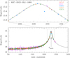 |
Fig. 1 Light curve of KMT-2023-BLG-1866. The lower panel provides a comprehensive view of the light curve, while the upper panel offers a magnified view of the top region. The color of each data point corresponds to the respective dataset indicated in the legend. The curve drawn over data points is a single-lens single source model. |
3 Light-curve modeling
Short-term central anomalies in the light curve of a high-magnification event can stem from three primary causes. Firstly, they may arise due to the presence of a planetary companion orbiting the lens, positioned approximately at the Einstein ring of the primary lens (Griest & Safizadeh 1998). Secondly, such anomalies can also result from a binary companion to the lens – in which the separation is notably different from the Einstein radius θE – being either significantly smaller or larger (An & Han 2002). A faint binary companion to the source can also create a transient central anomaly (Gaudi 1998). However, this particular channel results in a positive anomaly, prompting us to exclude this specific scenario from consideration.
To interpret the anomaly, we employed a binary-lens single-source (2L1S) model to analyze the light curve. The modeling was aimed at finding a set of lensing parameters (solution) that most accurately describe the observed light curve. Under the assumption that the relative motion between the lens and the source is rectilinear, a 2L1S lensing light curve is described by seven fundamental lensing parameters. The initial subset of these parameters (t0, u0, tE) characterizes the approach of the source to the lens. Each parameter denotes the time of closest approach, the separation between the lens and source at that specific time (impact parameter), and the event timescale. The event timescale is defined as the time required for the source to traverse the Einstein radius, that is, tE = θE/μ, where μ denotes the relative lens-source proper motion. The subsequent set of parameters (s, q, α) describe the binary-lens system itself and the direction of the source’s approach to the lens. These parameters represent the projected separation and mass ratio between the binary lens components M1 and M2 and the angle between the axis formed by M1 and M2 and the direction of μ vector, respectively. The lengths of u0 and s are scaled to θE. Finally, the parameter ρ is defined as the ratio of the angular source radius θ* to the Einstein radius, that is, ρ = θ*/θE (normalized source radius). This parameter characterizes the finite-source magnifications during instances when the source crosses or closely approaches lens caustics.
From the analyses of partially covered short-term central anomalies in three lensing events KMT-2021-BLG-2010, KMT-2022-BLG-0371, and KMT-2022-BLG-1013, Han et al. (2023b) recently showcased the intricacy of interpreting these signals due to the existence of multiple solutions affected by various types of degeneracies. To explore all potential degenerate solutions, our modeling approach commenced with grid searches for the binary lensing parameters s and q through multiple starting values of α. During this process, we iteratively minimized χ2 to determine the remaining lensing parameters. We achieved this using the Markov chain Monte Carlo (MCMC) method, employing an adaptive step size Gaussian sampler detailed in Doran & Mueller (2004). Interpreting a central anomaly observed in a high-magnification event can be complicated by the potential degeneracy between binary and planetary interpretations as demonstrated by Choi et al. (2012). To explore such degeneracies, we broadened the range for s and q to encompass both binary and planetary scenarios: −1.0 < log s < 1.0 and −6.0 < log q < 1.0. The parameter space was partitioned into 70 × 70 grids, with 21 initial values for the source trajectory angle α evenly distributed within the 0 < α ≤ 2π range. For the computation of finite-source magnifications, we utilized the map-making approach detailed by Dong et al. (2006). In our computations, we accounted for limb-darkening effects by modeling the surface brightness variation of the source as S ∝ 1 −Γ(1 − 3 cos ϕ/2), where Γ represents the limb-darkening coefficient and ϕ denotes the angle between the line extending from the source center to the observer and the line extending from the source center to the surface point. As we discuss in Sect. 4, the source star of the event is identified as a turnoff star of a mid-G spectral type. We adopted an I-band limb-darkening coefficient of ΓI = 0.45 from Claret (2000), under the assumption of an effective temperature of Teff = 5500 K, a surface gravity of log(g/g⊙) = −1.0, and a turbulence velocity of υturb = 2 km s−1. Following the identification of local solutions on the Δχ2 map in the log s-log q plane, we proceeded to refine the lensing parameters by gradually narrowing down the parameter space.
Figure 2 displays the Δχ2 map on the (log s, log q) parameter plane obtained from the grid search. The lower map shows entire grid of the inspected region, while the upper map displays a closer look at the area surrounding local solutions. From the investigation of the map, we identified three local solutions, which centered at (log s, log q) ~ (−0.015, −4.55), ~ (−0.009, −4.90), and ~ (−0.001, −4.55). We assign the individual solutions the labels “inner”, “intermediate”, and “outer”, with the rationale behind these designations discussed below. Regardless of the solutions, the estimated mass ratios are q < 10−4, suggesting that the anomaly was caused by a companion of very low mass associated with the lens.
Table 2 presents the complete lensing parameters for the three identified local solutions. The parameters of these solutions were refined from those obtained from the grid search by allowing unrestricted variation across all parameters and by considering higher order effects causing deviations of the relative lens-source motion from rectilinear. We examined two distinct higher order effects: the first arises from Earth’s orbital motion around the Sun, known as microlens-parallax effects (Gould 1992), while the second stems from the orbital motion of a planet around its host, referred to as lens-orbital effects (Batista et al. 2011; Skowron et al. 2011). For the consideration of the microlens-parallax effect, we added two lensing parameters (πE,N, πE,E), which denote the north and east components of the microlens-parallax vector πE, respectively. The microlensparallax vector is related to the distance to the lens DL and source DS; the relative parallax of the lens and source, πrel = au(1/DL − 1/DS); and the relative lens-source proper motion by
![Mathematical equation: $\[\boldsymbol{\pi}_{\mathrm{E}}=\left(\frac{\pi_{\mathrm{rel}}}{\theta_{\mathrm{E}}}\right)\left(\frac{\boldsymbol{\mu}}{\mu}\right).\]$](/articles/aa/full_html/2024/07/aa49618-24/aa49618-24-eq1.png) (1)
(1)
Under the assumption of a minor change in the lens configuration, we account for the lens-orbital effect by introducing two additional parameters (ds/dt, dα/dt), which represent the yearly rates of change in the binary separation and the angle of the source trajectory, respectively. Upon comparing the fits, it was observed that the degeneracies among the solutions are very severe with Δχ2 < 1.0.
In Fig. 3, we present the model curves of the three local solutions and their residuals in the region around the anomaly. The models are so alike that they are barely distinguishable within the line width. For all solutions, the anomaly is described by a dip feature surrounded by shallow hills appearing on both sides of the dip. According to the models, the two KMTC data points around HJD′ ~ 229.5 align with the dip feature’s valley, while the two MOA points at HJD′ = 229.89 and 229.97 correspond to the right-side hill.
The lens-system configurations corresponding to the individual solutions are depicted in Fig. 4. Across all solutions, the source consistently traversed the negative deviation region located behind the caustic positioned around the planet host. However, its specific alignment relative to the caustic differs among solutions. In the inner solution, the caustic consists of three segments, with one segment positioned near the planet’s host (central caustic) and the other two segments (the planetary caustic) situated away from the host, on the opposite side of the planet. The source trajectory passed through the inner area between these central and planetary caustics. Conversely, within the outer solution, the merging of the central and planetary caustics creates a unified resonant caustic. The source path crossed the outer region of this caustic. We classify these as inner and outer solutions, determined by the side of the caustic that the source passed through. In the intermediate solution, the caustic configuration resembles that of the inner solution; yet, in this case the source trajectory crossed the right side of the planetary caustic, unlike the trajectory of the inner solution.
The normalized source radius is measured, but the associated uncertainty varies depending on the solutions, as illustrated in the three upper panels of Fig. 5. These panels depict scatter plots of points in the MCMC chain on the u0−ρ parameter planes for the individual solutions. While the median values, ⟨ρ⟩ ~ 2 × 10⁻³, exhibit consistency across solutions, there is notable diversity in the corresponding uncertainties. Specifically, the uncertainty ranges from σ(ρ) ~ 0.18 × 10⁻³ for the intermediate solution to σ(ρ) ~ 0.61 × 10⁻³ for the outer solution. This variation arises due to disparities in the lens system configurations among the solutions.
It turned out that the similarity between the model curves of the inner and outer solutions was caused by the inner–outer degeneracy. This degeneracy was initially proposed by Gaudi & Gould (1997) to indicate the resemblance in planetary signals resulting from the source trajectories passing on near and far sides of a planetary caustic. Yee et al. (2021), Zhang et al. (2022), and Zhang & Gaudi (2022) later extended this concept to encompass planetary signals related to central and resonant caustics. Subsequently, Hwang et al. (2022) and Gould et al. (2022) proposed an analytical relationship between the lensing parameters of the pair of solutions affected by this degeneracy:
![Mathematical equation: $\[s_{ \pm}^{\dagger}=\sqrt{s_{\mathrm{in}} \times s_{\mathrm{out}}}=\frac{\sqrt{u_{\mathrm{anom}}^2+4} \pm u_{\mathrm{anom}}}{2}.\]$](/articles/aa/full_html/2024/07/aa49618-24/aa49618-24-eq2.png) (2)
(2)
Here, ![Mathematical equation: $\[u_{\text {anom }}^2=\tau_{\text {anom }}^2+u_0^2, \tau_{\text {anom }}=\left(t_{\text {anom }}-t_0\right) / t_{\mathrm{E}}\]$](/articles/aa/full_html/2024/07/aa49618-24/aa49618-24-eq3.png) , indicates the time of the anomaly, and sin and sout represent the planetary separations of the inner and outer solutions, respectively. For anomalies showing a bump feature, the sign in the right term is (+), whereas for those displaying a dip feature, the sign is (−). From the lensing parameters (t0, u0, tE, sin, sout, tanom) ~ (228.65, 3.3 × 10⁻², 75, 0.9740, 0.9894, 229.57), we find that the geometric mean
, indicates the time of the anomaly, and sin and sout represent the planetary separations of the inner and outer solutions, respectively. For anomalies showing a bump feature, the sign in the right term is (+), whereas for those displaying a dip feature, the sign is (−). From the lensing parameters (t0, u0, tE, sin, sout, tanom) ~ (228.65, 3.3 × 10⁻², 75, 0.9740, 0.9894, 229.57), we find that the geometric mean ![Mathematical equation: $\[\sqrt{s_{\text {in }} \times s_{\text {out }}}=0.982\]$](/articles/aa/full_html/2024/07/aa49618-24/aa49618-24-eq4.png) matches the value
matches the value ![Mathematical equation: $\[\left(\sqrt{u_{\text {anom }}^2+4} \pm u_{\text {anom }}\right) / 2=0.983\]$](/articles/aa/full_html/2024/07/aa49618-24/aa49618-24-eq5.png) very well.
very well.
Although the fit improvement from the static model is marginal, the microlens-parallax parameters could be constrained. This is demonstrated in the scatter plot of MCMC points within the (πE,E, πE,N) parameter plane, showcased in the lower panels of Fig. 5. Measuring these parameters is important because they offer constraints on the physical parameters of the lens (Gould 1992, 2000). In contrast, the determined orbital parameters exhibit considerable uncertainties.
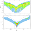 |
Fig. 2 Δχ2 map of (log s, log q) parameter plane obtained from the grid search. In the lower panel, the entire grid of the inspected region is displayed, while the upper panel provides a closer look at the area surrounding the three local solutions. Three identified local solutions are labeled as “inner”, “intermediate”, and “outer”. The color scheme is configured to represent points as red (<1n), yellow (<4n), green (<9n), and cyan (<16n). Here, n = 1 for the upper map and n = 10 for the lower map. |
Lensing parameters of three local solutions.
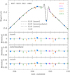 |
Fig. 3 Comparison of model curves of three identified local solutions (“inner”, “intermediate”, and “outer”) in the region of the anomaly. The model curves of the solutions are drawn over the data points in different line types. The lower three panels show the residuals from the individual solutions. The lensing parameters of the individual solutions are listed in Table 2, and the corresponding lens-system configurations are presented in Fig. 4. |
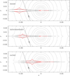 |
Fig. 4 Lens system configurations of three local solutions (“inner”, “intermediate”, and “outer”). In each panel, the figures drawn in red represent the caustic, and the line with an arrow denotes the source trajectory. The curves surrounding the caustics indicate the equi-magnification contours. The coordinates are centered at the position of the planet host. |
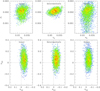 |
Fig. 5 Scatter plots of points in MCMC chain on u0−ρ (upper panels) and πE,E−πE,N (lower panels) parameter planes. The color scheme matches that utilized in Fig. 2. |
4 Source star and constraint on Einstein radius
In this section, we define the source star of the event. Defining the source is important not only to fully characterize the event, but also to estimate the angular Einstein radius. The value of the Einstein radius is constrained from the angular source radius by the relation
![Mathematical equation: $\[\theta_{\mathrm{E}}=\frac{\theta_*}{\rho},\]$](/articles/aa/full_html/2024/07/aa49618-24/aa49618-24-eq6.png) (3)
(3)
where the angular source radius θ* is deduced from the stellar type of the source.
The characterization of the source follows the methodology outlined in Yoo et al. (2004). Initially, we constructed the I- and V-band light curves of the event using the pyDIA code (Albrow 2017). Subsequently, we determined the flux values of the source, FS, in the individual pass bands by regressing the pyDIA light curves with respect to the lensing model, Amodel(t), that is,
![Mathematical equation: $\[F_{\text {obs }}(t)=A_{\text {model }}(t) F_{\mathrm{S}}(t)+F_{\mathrm{b}}.\]$](/articles/aa/full_html/2024/07/aa49618-24/aa49618-24-eq7.png) (4)
(4)
Here, Fobs(t) represents the observed flux of the event and Fb represents the flux contributed by blended stars. In the next step, we positioned the source in the instrumental color-magnitude diagram (CMD), which is constructed from the pyDIA photometry of stars located near the source. Finally, we converted the instrumental source color and magnitude, denoted as (V − I, I)S, into de-reddened values, (V − I, I)S,0. To do so, we utilized the centroid of the red giant clump (RGC) and its instrumental color and magnitude (V − I, I)RGC in the CMD as a reference; that is,
![Mathematical equation: $\[(V-I, I)_{\mathrm{S}, 0}=(V-I, I)_{\mathrm{RGC}, 0}+\Delta(V-I, I).\]$](/articles/aa/full_html/2024/07/aa49618-24/aa49618-24-eq8.png) (5)
(5)
Here, Δ(V − I, I) = (V − I, I)S − (V − I, I)RGC represents the offsets in color and magnitude of the source from those of the RGC centroid, and (V − I, I)RGC,0 = (1.060, 14.339) denote the de-reddened values of the RGC centroid, as determined by Bensby et al. (2013) and Nataf et al. (2013).
In Fig. 6, we mark the positions of the source (blue dot) and RGC centroid (red dot) in the instrumental CMD. The CMD is constructed from the pyDIA photometry of stars in the KMTC image lying 3.4 × 3.4 arcmin2 around the source. The estimated values of (V − I, I)S, (V − I, I)RGC, and (V − I, I)S,0 are detailed in Table 3. Based on the de-reddened color and magnitude, the source is identified as a turnoff star of a mid-G spectral type. For the estimation of the angular source radius, we first converted the measured V − I color into V − K color using the Bessell & Brett (1988) relation, and then we deduced θ* from the Kervella et al. (2004) relation between (V − K, I) and θ*. The estimated angular source radius from this process is
![Mathematical equation: $\[\theta_*=0.837 \pm 0.083 \mu \mathrm{as}.\]$](/articles/aa/full_html/2024/07/aa49618-24/aa49618-24-eq9.png) (6)
(6)
When combined with the normalized source radii associated with the distinct degenerate solutions presented in Table 2, this provides the Einstein radii corresponding to the individual solutions of
![Mathematical equation: $\[\theta_{\mathrm{E}}=\frac{\theta_*}{\rho}= \begin{cases}0.367 \pm 0.070 \mathrm{~mas} & \text { (inner), } \\ 0.420 \pm 0.057 \mathrm{~mas} & \text { (intermediate), } \\ 0.371 \pm 0.107 \mathrm{~mas} & \text { (outer), }\end{cases}\]$](/articles/aa/full_html/2024/07/aa49618-24/aa49618-24-eq10.png) (7)
(7)
and the values of relative lens-source proper motion of
![Mathematical equation: $\[\mu=\frac{\theta_{\mathrm{E}}}{t_{\mathrm{E}}}= \begin{cases}1.79 \pm 0.34 \mathrm{~mas} \mathrm{~yr}^{-1} & \text { (inner), } \\ 1.99 \pm 0.27 \mathrm{~mas} \mathrm{~yr}^{-1} & \text { (intermediate), } \\ 1.82 \pm 0.52 \mathrm{~mas} \mathrm{~yr}^{-1} & \text { (outer). }\end{cases}\]$](/articles/aa/full_html/2024/07/aa49618-24/aa49618-24-eq11.png) (8)
(8)
As we describe here, the blended light (formally fb = 0.038 ± 0.019) is not reliably detected. That is, it is consistent with zero. We can use this non-detection to place limits on the lens light. There are three sources of uncertainty in the measurement of the blend light. The first is the formal uncertainty from the fit, in which the baseline flux is formally treated as perfectly measured: σformal = 0.019. The second is the photon error in the measurement of the baseline flux σbase = 0.025. The quadrature sum of these is ![Mathematical equation: $\[\sigma_{\text {naive }}=\left(\sigma_{\text {formal }}^2+\sigma_{\text {base }}^2\right)^{1 / 2}=0.031\]$](/articles/aa/full_html/2024/07/aa49618-24/aa49618-24-eq12.png) , which is equivalent to an Inaive = 21.8 star. This is far below the error due to the mottled background of unresolved stars (Park et al. 2004). Because this field is far from the Galactic plane and center and so is very sparse, we conservatively estimated the 3 σ upper limit on the lens flux due to mottled background as fL < 0.25 or
, which is equivalent to an Inaive = 21.8 star. This is far below the error due to the mottled background of unresolved stars (Park et al. 2004). Because this field is far from the Galactic plane and center and so is very sparse, we conservatively estimated the 3 σ upper limit on the lens flux due to mottled background as fL < 0.25 or
![Mathematical equation: $\[I_{\mathrm{L}}>19.5.\]$](/articles/aa/full_html/2024/07/aa49618-24/aa49618-24-eq13.png) (9)
(9)
We note that this constraint eliminates roughly half of lens distribution that would be obtained in its absence, and thus it is highly significant.
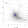 |
Fig. 6 Positions of source (blue dot) and red-giant-clump (RGC: red dot) centroid in the instrumental color–magnitude diagram of stars adjacent to the source star. |
Source parameters.
5 Physical lens parameters
We determine the physical lens parameters through a Bayesian analysis that integrates constraints from measured lensing observables with priors derived from the physical and dynamical distributions, along with the mass function of lens objects within the Milky Way. This analysis begins by generating numerous synthetic events via Monte Carlo simulation. Each event’s mass (Mi) was derived from a model mass function, and the distances to the lens and source (DL,i, DS,i), alongside their relative proper motion (μi), were inferred using a Galaxy model. Our simulation incorporates the mass-function model proposed by Jung et al. (2018) and utilizes the Galaxy model introduced in Jung et al. (2021). The bulge density profile in the Galaxy model conform to the triaxial model described by Han & Gould (1995), while the density profile of disk objects adheres to the modified double-exponential form as presented in Table 3 of their paper. In the mass function, we did not include stellar remnants because the formation of planets around stellar remnants is considered less probable due to disruptive events associated with these stellar objects. Subsequently, we calculated the timescale and Einstein radius of each synthetic event using relations represented by
![Mathematical equation: $\[t_{\mathrm{E}, i}=\frac{\theta_{\mathrm{E}, i}}{\mu_i} \quad \text { and } \quad \theta_{\mathrm{E}, i}=\sqrt{\kappa M_i \pi_{\mathrm{rel}, i}} \text {, }\]$](/articles/aa/full_html/2024/07/aa49618-24/aa49618-24-eq14.png) (10)
(10)
where κ = 4G/(c2au) = 8.14 mas/M⊙. The microlens parallax was computed using the relation presented in Eq. (1). In the subsequent step, we assigned a weight to each event proportional of
![Mathematical equation: $\[w_i=\exp \left(\frac{\chi_i^2}{2}\right),\]$](/articles/aa/full_html/2024/07/aa49618-24/aa49618-24-eq15.png) (11)
(11)
where the ![Mathematical equation: $\[\chi_i^2\]$](/articles/aa/full_html/2024/07/aa49618-24/aa49618-24-eq16.png) value was computed using the relation
value was computed using the relation
![Mathematical equation: $\[\begin{aligned}\chi_i^2= & \frac{\left(t_{\mathrm{E}, i}-t_{\mathrm{E}}\right)}{\sigma^2\left(t_{\mathrm{E}}\right)}+\frac{\left(\theta_{\mathrm{E}, i}-\theta_{\mathrm{E}}\right)}{\sigma^2\left(\theta_{\mathrm{E}}\right)} \\& +\sum_{j=1}^2 \sum_{k=1}^2 b_{j, k}\left(\pi_{\mathrm{E}, j, i}-\pi_{\mathrm{E}, i}\right)\left(\pi_{\mathrm{E}, k, i}-\pi_{\mathrm{E}, i}\right).\end{aligned}\]$](/articles/aa/full_html/2024/07/aa49618-24/aa49618-24-eq17.png) (12)
(12)
Here, [tE, σ(tE)] and [θE, σ(θE)] denote the measured timescale and Einstein radius and their uncertainty, respectively, and bj,k represents the inverse covariance matrix of the microlensparallax vector πE. (πE,1, πE,2)i = (πE,N, πE,E)i represent the parallax parameters of each simulated event, while (πE,N, πE,E) denotes the measured parallax parameters.
Aside from the constraint provided by the lensing observables, we incorporated an additional constraint derived from the blended flux. This constraint is rooted in the relationship between the lens flux and the overall blended flux, requiring the lens flux to be lower than the total blending flux. To compute the I-band magnitude of the lens, we utilized the following equation:
![Mathematical equation: $\[I_{\mathrm{L}}=M_{I, \mathrm{~L}}+5 \log \left(\frac{D_{\mathrm{L}}}{\mathrm{pc}}\right)-5+A_{I, \mathrm{~L}}.\]$](/articles/aa/full_html/2024/07/aa49618-24/aa49618-24-eq18.png) (13)
(13)
Here, MI,L denotes the absolute magnitude of the lens, and AI,L represents the extinction at a distance DL. For the derivation of absolute magnitude MI,L corresponding the lens mass, we used the Pecaut & Mamajek (2013) mass–luminosity relation, which was derived from pre-main-sequence stars in nearby, negligibly reddened stellar groups. The extinction is modeled as
![Mathematical equation: $\[A_{I, \mathrm{~L}}=A_{I, \text {tot }}\left[1-\exp -\left(\frac{|z|}{h_{z, \text {dust }}}\right)\right],\]$](/articles/aa/full_html/2024/07/aa49618-24/aa49618-24-eq19.png) (14)
(14)
where AI,tot = 0.46 indicates the overall extinction observed in the field, hz,dust = 100 pc represents the dust’s scale height, z = DL sin b + z0 and z0 = 15 pc denote the heights of the lens and the Sun above the Galactic plane, respectively. We note that dust may be distributed unevenly in patches, and therefore our model, which assumes a smooth distribution, provides only an approximate description of the dust. We enforced the blending constraint by assigning a weight wi = 0 to artificial events featuring lenses whose brightness fails to meet the condition specified in Eq. (9). It turns out that the blending constraint has a significant impact on the estimation of lens parameters.
Figure 7 shows the posteriors of the primary lens mass and distance to the lens. Table 4 presents the estimated host mass (Mhost), planet mass (Mplanet), distance (DL) to the planetary system, and projected planet-host separation (a⊥ = sθEDL) corresponding to the individual degenerate solutions. The median of each posterior distribution was chosen as the representative value, while the uncertainties were quantified by 16% and 84% of the distribution. Based on the estimated mass, the host of the planet is identified as a low-mass star of an early M spectral type. The estimated mass of the planet falls within the range of approximately 2.6 to 4.0 times Earth’s mass in terms of the median value, signifying a notably low mass. Positioned at a distance of about (6.2–6.5) kpc from Earth, this planetary system resides in a region where approximately 85% of the stellar population belongs to the Galactic bulge, with the remaining 15% being in the disk. The projected separation between the planet and its host star is approximately 2.5 au, which is roughly two times farther than the ice-line distance.
The identification of planet KMT-2023-BLG-1866Lb is of significant scientific importance due to its remarkably low mass. Despite the growing planet detection efficiency of lensing experiments, planets falling into the categories of terrestrial planets (with masses ≲2 ME) and super-Earths (with masses around ~3–10 ME) still represent a small fraction of the microlensing planets. KMT-2023-BLG-1866Lb occupies a region of very low mass, where planets are sparsely distributed, as depicted in Fig. 8. Therefore, its detection signifies the extension of the lensing surveys to very-low-mass planets that were difficult to detect in earlier surveys.
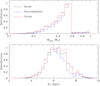 |
Fig. 7 Bayesian posteriors of primary lens mass (Mhost) and distance to the lens (DL). In each panel, three curves drawn in black, blue, and red represent posteriors corresponding to the inner, intermediate, and outer solutions, respectively. |
Physical lens parameters.
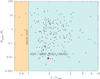 |
Fig. 8 Distribution of microlensing planets in parameter space defined by their mass and projected separation. The separation is scaled to the snow line of the planet host, which is represented by a vertical line. The red dot indicates the location of KMT-2023-BLG-1866Lb. |
6 Summary
We investigated the nature of the brief anomaly observed close to the peak of the lensing light curve in KMT-2023-BLG-1866. This anomaly was partially covered, primarily because of its short duration, cloudy weather conditions at the observation sites, and limited nighttime availability toward the end of the bulge season. To address the inherent challenges of interpreting partially covered signals, we conducted a rigorous exploration of all plausible degenerate solutions. This in-depth analysis revealed three distinct planetary scenarios that provide equally valid explanations for the observed anomaly. These scenarios are characterized by the specific planetary parameters: (s, q)inner = [0.9740 ± 0.0083, (2.46 ± 1.07) × 10−5], (s, q)intermediate = [0.9779 ± 0.0017, (1.56 ± 0.25) × 10−5], and (s, q)outer = [0.9894 ± 0.0107, (2.31 ± 1.29) × 10−5]. We identified that the ambiguity between the inner and outer solutions stems from the inner-outer degeneracy, while the similarity between the intermediate solution and the others is due to an accidental degeneracy caused by incomplete anomaly coverage. Through a Bayesian analysis utilizing the constraints derived from measured lensing observables and blending flux, our estimation indicates that the lens system comprises a very-low-mass planet orbiting an early M-type star situated approximately (6.2–6.5) kpc from Earth in terms of median posterior values for the different solutions. The median mass of the planet host is in the range of (0.48–0.51) M⊙, and that of the planet’s mass spans a range of (2.6–4.0) ME, which varies across different solutions.
Acknowledgements
Work by C.H. was supported by the grants of National Research Foundation of Korea (2019R1A2C2085965). J.C.Y. and I.-G.S. acknowledge support from U.S. NSF Grant No. AST-2108414. Y.S. acknowledges support from BSF Grant No. 2020740. This research has made use of the KMTNet system operated by the Korea Astronomy and Space Science Institute (KASI) at three host sites of CTIO in Chile, SAAO in South Africa, and SSO in Australia. Data transfer from the host site to KASI was supported by the Korea Research Environment Open NETwork (KREONET). This research was supported by KASI under the R&D program (Project No. 2024-1-832-01) supervised by the Ministry of Science and ICT. W.Z. and H.Y. acknowledge support by the National Natural Science Foundation of China (Grant No. 12133005). W. Zang acknowledges the support from the Harvard-Smithsonian Center for Astrophysics through the CfA Fellowship. The MOA project is supported by JSPS KAKENHI Grant Number JP24253004, JP26247023, JP16H06287 and JP22H00153.
References
- Albrow, M. 2017, https://doi.org/10.5281/zenodo.268049 [Google Scholar]
- Albrow, M., Horne, K., Bramich, D. M., et al. 2009, MNRAS, 397, 2099 [Google Scholar]
- Alcock, C., Akerlof, C. W., Allsman, R. A., et al. 1993, Nature, 365, 621 [NASA ADS] [CrossRef] [Google Scholar]
- An, J. H., & Han, C. 2002, ApJ, 573, 351 [NASA ADS] [CrossRef] [Google Scholar]
- Aubourg, E., Bareyre, P., Bréhin, S., et al. 1993, Nature, 365, 623 [NASA ADS] [CrossRef] [Google Scholar]
- Batista, V., Gould, A., Dieters, S. et al. 2011, A&A, 529, A102 [NASA ADS] [CrossRef] [EDP Sciences] [Google Scholar]
- Beaulieu, J.-P., Bennett, D. P., Fouqué, P., et al. 2006, Nature, 439, 437 [Google Scholar]
- Bell, A., Zhang, J., Zang. W. et al. 2024, PASP, 136, 054402 [NASA ADS] [CrossRef] [Google Scholar]
- Bensby, T., Yee, J. C., Feltzing, S., et al. 2013, A&A, 549, A147 [NASA ADS] [CrossRef] [EDP Sciences] [Google Scholar]
- Bessell, M. S., & Brett, J. M. 1988, PASP, 100, 1134 [Google Scholar]
- Bond, I. A., Abe, F., Dodd, R. J., et al. 2001, MNRAS, 327, 868 [Google Scholar]
- Bond, I. A., Udalski, A., Jaroszyński, M., et al. 2004, ApJ, 606, L155 [NASA ADS] [CrossRef] [Google Scholar]
- Choi, J.-Y., Shin, I.-G., Han, C., et al. 2012, ApJ, 756, 48 [Google Scholar]
- Claret, A. 2000, A&A, 363, 1081 [NASA ADS] [Google Scholar]
- Dong, S., DePoy, D. L., Gaudi, B. S., et al. 2006, ApJ, 642, 842 [NASA ADS] [CrossRef] [Google Scholar]
- Doran, M., & Mueller, C. M. 2004, J. Cosmol. Astropart. Phys., 09, 003 [CrossRef] [Google Scholar]
- Gaudi, B. S. 1998, ApJ, 506, 533 [Google Scholar]
- Gaudi, B. S., & Gould, A. 1997, ApJ, 486, 85 [Google Scholar]
- Gould, A. 1992, ApJ, 392, 442 [Google Scholar]
- Gould, A. 2000, ApJ, 542, 785 [NASA ADS] [CrossRef] [Google Scholar]
- Gould, A., & Loeb, A. 1992, ApJ, 396, 104 [Google Scholar]
- Gould, A., Udalski, A., An, D., et al. 2006, ApJ, 644, L37 [Google Scholar]
- Gould, A., Udalski, A., Shin, I.-G., et al. 2014, Science, 345, 46 [Google Scholar]
- Gould, A., Ryu, Y.-H., Calchi Novati, S., et al. 2020, JKAS, 53, 9 [NASA ADS] [Google Scholar]
- Gould, A., Han, C., Zang, W., et al. 2022, A&A, 664, A13 [NASA ADS] [CrossRef] [EDP Sciences] [Google Scholar]
- Griest, K., & Safizadeh, N. 1998, ApJ, 500, 37 [Google Scholar]
- Han, C., & Gould, A. 1995, ApJ, 447, 53 [Google Scholar]
- Han, C., Udalski, A., Lee, C.-U., et al. 2021, A&A, 649, A90 [EDP Sciences] [Google Scholar]
- Han, C., Gould, A., Albrow, M. D., et al. 2022a, A&A, 658, A62 [NASA ADS] [CrossRef] [EDP Sciences] [Google Scholar]
- Han, C., Bond, I. A., Yee, J. C., et al. 2022b, A&A, 658, A94 [NASA ADS] [CrossRef] [EDP Sciences] [Google Scholar]
- Han, C., Kim, D., Gould, A., et al. 2022c, A&A, 664, A33 [NASA ADS] [CrossRef] [EDP Sciences] [Google Scholar]
- Han, C., Gould, A., Jung, Y. K., et al. 2023a, A&A, 674, A89 [NASA ADS] [CrossRef] [EDP Sciences] [Google Scholar]
- Han, C., Lee, C.-U., Zang, W., et al. 2023b, A&A, 674, A90 [NASA ADS] [CrossRef] [EDP Sciences] [Google Scholar]
- Herrera-Martín, A., Albrow, M. D., Udalski, A. et al. 2020, AJ, 159, 256 [Google Scholar]
- Hwang, K. H., Kim, H. W., Kim, D. J., et al. 2018a, JKAS, 51, 197 [NASA ADS] [Google Scholar]
- Hwang, K.-H., Udalski, A., Shvartzvald, Y., et al. 2018b, AJ, 155, 20 [Google Scholar]
- Hwang, K.-H., Zang, W., Gould, A., et al. 2022, AJ, 163, 43 [NASA ADS] [CrossRef] [Google Scholar]
- Jung, Y. K., Udalski, A., Gould, A., et al. 2018, AJ, 155, 219 [Google Scholar]
- Jung, Y. K., Udalski, A., Zang, W., et al. 2020, AJ, 160, 255 [Google Scholar]
- Jung, Y. K., Han, C., Udalski, A., et al. 2021, AJ, 161, 293 [NASA ADS] [CrossRef] [Google Scholar]
- Kervella, P., Thévenin, F., Di Folco, E., & Ségransan, D. 2004, A&A, 426, 29 [Google Scholar]
- Kim, S.-L., Lee, C.-U., Park, B.-G., et al. 2016, JKAS, 49, 37 [Google Scholar]
- Kondo, I., Yee, J. C., Bennett, D. P., et al. 2021, AJ, 162, 77 [NASA ADS] [CrossRef] [Google Scholar]
- Mao, S., & Paczyński, B. 1991, ApJ, 374, L37 [Google Scholar]
- Muraki, Y., Han, C., Bennett, D. P., et al. 2011, ApJ, 741, 22 [Google Scholar]
- Nataf, D. M., Gould, A., Fouqué, P., et al. 2013, ApJ, 769, 88 [Google Scholar]
- Paczyński, B. 1986, ApJ, 304, 1 [NASA ADS] [CrossRef] [Google Scholar]
- Park, B.-G., DePoy, D. L., Gaudi, B. S., et al. 2004, ApJ, 609, 166 [NASA ADS] [CrossRef] [Google Scholar]
- Pecaut, M. J., & Mamajek, E. E. 2013, ApJS, 208, 9 [Google Scholar]
- Ranc, C., Bennett, D. P., Hirao, Y., et al. 2019, AJ, 157, 232 [NASA ADS] [CrossRef] [Google Scholar]
- Robin, A. C., Reyle, C., Derriére, S., & Picaud, S. 2003, A&A, 409, 523 [NASA ADS] [CrossRef] [EDP Sciences] [Google Scholar]
- Ryu, Y.-H., Udalski, A., Yee, J. C., et al. 2020, AJ, 160, 183 [Google Scholar]
- Ryu, Y.-H., Jung, Y. K., Yang, H., et al. 2022, AJ, 164, 180 [CrossRef] [Google Scholar]
- Sumi, T., Bennett, D. P., Bond, I. A., et al. 2010, ApJ, 710, 1641 [Google Scholar]
- Shvartzvald, Y., Yee, J. C., Novati, S. C., et al. 2017, ApJ, 840, L3 [NASA ADS] [CrossRef] [Google Scholar]
- Skowron, J., Udalski, A., Gould, A., et al. 2011, ApJ, 738, 87 [Google Scholar]
- Udalski, A. 2003, Acta Astron., 53, 291 [NASA ADS] [Google Scholar]
- Udalski, A., Szymański, M., Kałużny, J., et al. 1994, Acta Astron., 44, 1 [Google Scholar]
- Udalski, A., Szymański, M. K., Szymański, G., et al. 2015, Acta Astron., 65, 1 [NASA ADS] [Google Scholar]
- Udalski, A., Ryu, Y.-H., Sajadian, S., et al. 2018, Acta Astron., 68, 1 [Google Scholar]
- Yang, H., Zang, W., Gould, A., et al. 2022, MNRAS, 516, 1894 [NASA ADS] [CrossRef] [Google Scholar]
- Yang, H., Yee, J. C., Hwang, K.-H., et al. 2024, MNRAS, 528, 11 [NASA ADS] [CrossRef] [Google Scholar]
- Yee, J. C., Shvartzvald, Y., Gal-Yam, A., et al. 2012, ApJ, 755, 102 [Google Scholar]
- Yee, J. C., Zang, W., Udalski, A., et al. 2021, AJ, 162, 180 [NASA ADS] [CrossRef] [Google Scholar]
- Yoo, J., DePoy, D. L., Gal-Yam, A., et al. 2004, ApJ, 603, 139 [Google Scholar]
- Zang, W., Hwang, K.-H., Udalski, A., et al. 2021a, AJ, 162, 163 [NASA ADS] [CrossRef] [Google Scholar]
- Zang, W., Han, C., Kondo, I., et al. 2021b, Res. Astro. and Astroph., 21, 239 [CrossRef] [Google Scholar]
- Zang, W., Jung, Y. K., Yang, H., et al. 2023, AJ, 165, 103 [CrossRef] [Google Scholar]
- Zhang, K., & Gaudi, B. S. 2022, ApJ, 936, L22 [NASA ADS] [CrossRef] [Google Scholar]
- Zhang, K., Gaudi, B. S., & Bloom, J. S. 2022, Nat Astron, 6., 782 [NASA ADS] [CrossRef] [Google Scholar]
- Zhang, J., Zang, W., Jung, Y. K., et al. 2023, MNRAS, 522, 6055 [NASA ADS] [CrossRef] [Google Scholar]
KMT-2016-BLG-0212 (Hwang et al. 2018a), KMT-2016-BLG-1105 (Zang et al. 2023), OGLE-2016-BLG-1195 (Shvartzvald et al. 2017), KMT-2017-BLG-1003 (Zang et al. 2023), KMT-2017-BLG-0428 (Zang et al. 2023), KMT-2017-BLG-1194 (Zang et al. 2023), OGLE-2017-BLG-0173 (Hwang et al. 2018b), OGLE-2017-BLG-1434 (Udalski et al. 2018), OGLE-2017-BLG-1691 (Han et al. 2022c), OGLE-2017-BLG-1806 (Zang et al. 2023), KMT-2018-BLG-0029 (Gould et al. 2020), KMT-2018-BLG-1025 (Han et al. 2021), KMT-2018-BLG-1988 (Han et al. 2022a), OGLE-2018-BLG-0506 (Hwang et al. 2022), OGLE-2018-BLG-0532 (Ryu et al. 2020), OGLE-2018-BLG-0977 (Hwang et al. 2022), OGLE-2018-BLG-1185 (Kondo et al. 2021), OGLE-2018-BLG-1126 (Gould et al. 2022), KMT-2019-BLG-0253 (Hwang et al. 2022), KMT-2019-BLG-0842 (Jung et al. 2020), KMT-2019-BLG-1367 (Zang et al. 2023), KMT-2019-BLG-1806 (Zang et al. 2023), OGLE-2019-BLG-0960 (Yee et al. 2021), and OGLE-2019-BLG-1053 (Zang et al. 2021a).
The photometry data are available through the following web page: http://astroph.chungbuk.ac.kr/~cheongho/KMT-2023-BLG-1866/data.html.
All Tables
All Figures
|
Fig. 1 Light curve of KMT-2023-BLG-1866. The lower panel provides a comprehensive view of the light curve, while the upper panel offers a magnified view of the top region. The color of each data point corresponds to the respective dataset indicated in the legend. The curve drawn over data points is a single-lens single source model. |
| In the text | |
|
Fig. 2 Δχ2 map of (log s, log q) parameter plane obtained from the grid search. In the lower panel, the entire grid of the inspected region is displayed, while the upper panel provides a closer look at the area surrounding the three local solutions. Three identified local solutions are labeled as “inner”, “intermediate”, and “outer”. The color scheme is configured to represent points as red (<1n), yellow (<4n), green (<9n), and cyan (<16n). Here, n = 1 for the upper map and n = 10 for the lower map. |
| In the text | |
|
Fig. 3 Comparison of model curves of three identified local solutions (“inner”, “intermediate”, and “outer”) in the region of the anomaly. The model curves of the solutions are drawn over the data points in different line types. The lower three panels show the residuals from the individual solutions. The lensing parameters of the individual solutions are listed in Table 2, and the corresponding lens-system configurations are presented in Fig. 4. |
| In the text | |
|
Fig. 4 Lens system configurations of three local solutions (“inner”, “intermediate”, and “outer”). In each panel, the figures drawn in red represent the caustic, and the line with an arrow denotes the source trajectory. The curves surrounding the caustics indicate the equi-magnification contours. The coordinates are centered at the position of the planet host. |
| In the text | |
|
Fig. 5 Scatter plots of points in MCMC chain on u0−ρ (upper panels) and πE,E−πE,N (lower panels) parameter planes. The color scheme matches that utilized in Fig. 2. |
| In the text | |
|
Fig. 6 Positions of source (blue dot) and red-giant-clump (RGC: red dot) centroid in the instrumental color–magnitude diagram of stars adjacent to the source star. |
| In the text | |
|
Fig. 7 Bayesian posteriors of primary lens mass (Mhost) and distance to the lens (DL). In each panel, three curves drawn in black, blue, and red represent posteriors corresponding to the inner, intermediate, and outer solutions, respectively. |
| In the text | |
|
Fig. 8 Distribution of microlensing planets in parameter space defined by their mass and projected separation. The separation is scaled to the snow line of the planet host, which is represented by a vertical line. The red dot indicates the location of KMT-2023-BLG-1866Lb. |
| In the text | |
Current usage metrics show cumulative count of Article Views (full-text article views including HTML views, PDF and ePub downloads, according to the available data) and Abstracts Views on Vision4Press platform.
Data correspond to usage on the plateform after 2015. The current usage metrics is available 48-96 hours after online publication and is updated daily on week days.
Initial download of the metrics may take a while.