| Issue |
A&A
Volume 698, June 2025
|
|
|---|---|---|
| Article Number | A292 | |
| Number of page(s) | 21 | |
| Section | Numerical methods and codes | |
| DOI | https://doi.org/10.1051/0004-6361/202453377 | |
| Published online | 24 June 2025 | |
Automated quasar continuum estimation using neural networks
A comparative study of deep-learning architectures
1
Dipartimento di Fisica ‘G. Occhialini’, Università degli Studi di Milano-Bicocca,
Piazza della Scienza 3,
20126
Milano,
Italy
2
National Centre for Nuclear Research,
ul. Pasteura 7,
02-093
Warsaw,
Poland
3
INAF – Osservatorio di Astrofisica e Scienza dello Spazio di Bologna,
Via Piero Gobetti 93/3,
40129
Bologna,
Italy
4
INAF – Osservatorio Astronomico di Trieste,
via G.B. Tiepolo 11,
34143
Trieste,
Italy
5
INAF – Osservatorio Astronomico di Brera,
Via Brera 28, 20122 Milano, via E. Bianchi 46,
23807
Merate,
Italy
6
NRC Herzberg Astronomy and Astrophysics Research Centre,
5071 West Saanich Road,
Victoria,
B.C.
V9E 2E7,
Canada
7
Department of Physics and Astronomy Camosun College,
3100 Foul Bay Rd,
Victoria,
B.C.
V8P 5J2,
Canada
8
Aix Marseille Univ. CNRS, CNES, LAM,
Marseille,
France
9
IUCAA, Postbag 4, Ganeshkind,
Pune
411007,
India
10
Department of Astronomy, University of Illinois at Urbana-Champaign,
Urbana,
IL
61801,
USA
11
Institute of Astronomy, University of Cambridge,
Madingley Road,
Cambridge
CB3 0HA,
UK
12
Instituto de Astrofisica, Facultad de Fisica, Pontificia Universidad Catolica de Chile,
Santiago,
Chile
13
Departament de Fisica, EEBE, Universitat Politécnica de Catalunya,
c/Eduard Maristany 10,
08930
Barcelona,
Spain
14
Astronomical Observatory of the Jagiellonian University,
Orla 171,
30-001
Cracow,
Poland
★ Corresponding author: This email address is being protected from spambots. You need JavaScript enabled to view it.
Received:
10
December
2024
Accepted:
16
May
2025
Abstract
Context. Ongoing and upcoming large spectroscopic surveys are drastically increasing the number of observed quasar spectra, making the development of fast and accurate automated methods to estimate spectral continua necessary.
Aims. This study evaluates the performance of three neural networks (NNs) – an autoencoder, a convolutional NN (CNN), and a U-Net – in predicting quasar continua within the rest frame wavelength range of 1020 Å to 2000 Å. The ability to generalize and predict galaxy continua within the range of 3500 Å to 5500 Å is also tested.
Methods. We evaluated the performance of these architectures using the absolute fractional flux error (AFFE) on a library of mock quasar spectra for the WEAVE survey and on real data from the early data release observations of the Dark Energy Spectroscopic Instrument (DESI) and the VIMOS Public Extragalactic Redshift Survey (VIPERS).
Results. The autoencoder outperforms U-Net, achieving a median AFFE of 0.009 for quasars. The best model also effectively recovers the Lyα optical depth evolution in the DESI quasar spectra. With minimal optimization, the same architectures can be generalized to the galaxy case, with the autoencoder reaching a median AFFE of 0.014 and reproducing the D4000n break in DESI and VIPERS galaxies.
Key words: methods: data analysis / galaxies: general / intergalactic medium / quasars: absorption lines / quasars: general / large-scale structure of Universe
© The Authors 2025
 Open Access article, published by EDP Sciences, under the terms of the Creative Commons Attribution License (https://creativecommons.org/licenses/by/4.0), which permits unrestricted use, distribution, and reproduction in any medium, provided the original work is properly cited.
This article is published in open access under the Subscribe to Open model. This email address is being protected from spambots. You need JavaScript enabled to view it. to support open access publication.
1 Introduction
Quasars are important probes of the distribution of baryonic matter, which is imprinted on the spectra in the form of absorption lines. For example, the distribution of neutral hydrogen in the intergalactic medium (IGM) is observed as a dense forest of absorbers at wavelengths lower than 1216 Å in the quasar rest frame, the so-called Lyman-α forest (Lyα; Lynds 1971; Bahcall & Goldsmith 1971; McDonald et al. 2006; Shull et al. 2012). Hydrodynamical simulations contributed to the interpretation of the Lyα forest, showing that hydrogen follows the underlying dark matter distribution in the network of filaments, voids, and clusters (Cen et al. 1994; Hernquist et al. 1996; Croft et al. 1998). At the same time, at wavelengths λ > 1216 Å in the quasar rest frame, spectroscopy offers a detailed view of the composition and kinematics of the diffuse, metal-enriched gas (through the measurements of absorption lines such as CIV, MgII, and SiIV; Dutta et al. 2020; Galbiati et al. 2023) between and near galaxies, within the circumgalactic medium (CGM). High-quality estimates for the quasar continua are required to measure the optical depth of the transitions producing the absorption lines and hence extract physical information from these datasets.
Likewise, galaxy spectra provide critical information about how the gas in the CGM is eventually converted and processed within the interstellar medium (ISM) and stars. These transformations are imprinted in relations such as the mass-metallicity relation (Erb et al. 2010; Wuyts et al. 2012; Zahid et al. 2014; Bian et al. 2017) or the fundamental metallicity relation (Mannucci et al. 2010; Cresci et al. 2019; Curti et al. 2020; Pistis et al. 2022, 2024). To have a reliable measurement of the absorption and emission features (e.g., the metallicity derived as the relative abundance of oxygen to hydrogen), it is, once again, essential to accurately determine the continuum of the galaxy spectra. Moreover, the continua of galaxies contain a plethora of information about the stellar population (Maraston 2005; Maraston & Strömbäck 2011; Vazdekis et al. 2010).
The increasing amount of data since the advent of big spectroscopic surveys such as the Sloan Digital Sky Survey (SDSS; Abazajian et al. 2009), the VIMOS Public Extragalactic Redshift Survey (VIPERS; Scodeggio et al. 2018), the Dark Energy Spectroscopic Instrument (DESI Collaboration 2022), and the ESA Euclid mission (Laureijs et al. 2011), or the upcoming WHT Enhanced Area Velocity Explorer (WEAVE; Dalton et al. 2012, 2014, 2016; Pieri et al. 2016; Jin et al. 2024) and the 4-meter Multi-Object Spectroscopic Telescope (4MOST; de Jong et al. 2019) make the estimate of continuum spectra an untractable problem with traditional continuum fitting techniques based on, for example, minimization of the χ2 or via fitting of stellar population synthesis (SPS) models. Thus, it is necessary to resort to fully automatic algorithms suitable for accurate and precise measurements in large catalogs using a limited amount of computational time and resources.
In this context, machine learning (ML) has emerged as a powerful tool to approach the challenges of continuum fitting. Various ML algorithms have been developed with different applications to astrophysical spectra, including classification of the sources (Folkes et al. 1996; Geach 2012; Pat et al. 2022; Wang et al. 2023; Abraham et al. 2024; Wu et al. 2024); redshift measurements (Machado et al. 2013; Giri et al. 2020); analysis of lines both in emission (Bégué et al. 2024) and absorption (Jalan et al. 2024); or stellar population (Liew-Cain et al. 2021; Murata & Takeuchi 2022; Wang et al. 2024). ML algorithms can automatically learn complex patterns from large amounts of data, making them ideal for processing the extensive datasets generated by modern spectroscopic surveys. For example, neural networks (NNs) and other ML techniques can be trained to predict the quasar continuum by learning from a substantial number of spectra. This approach can accommodate the broad emission lines and the intricate shape of the quasar continuum on the red and blue sides of the Lyα emission (Pâris et al. 2011; Greig et al. 2017), as well as the complexity of galaxy spectra (Portillo et al. 2020; Teimoorinia et al. 2022; Melchior et al. 2023; Böhm et al. 2023; Liang et al. 2023a,b).
Considering quasars, which are the main focus of this study, early explorations of this approach include the prediction of the true continuum using only the red part of the spectra (redward of the Lyα line) using principal component analysis (PCA; Suzuki et al. 2005; Pâris et al. 2011; Lee et al. 2012; Davies et al. 2018). However, additional constraints on the α mean flux (Lee et al. 2012) are often required to improve the predictions in the forest region. ML models offer a more flexible and potentially more accurate alternative by directly learning the relationship between different spectral regions and the underlying continuum, reducing the need for such corrections. Recently, efforts have moved toward a deep-learning approach. For example, a feedforward NN (such as an autoencoder) shows good results predicting the quasar continuum in the Lyα forest region when using as input only information on the red side of the spectra (Liu & Bordoloi 2021). Another approach is to use a convolutional NN (CNN). This kind of architecture shows, on average, lower errors than the feedforward NN (Turner et al. 2024). A similar direction has been taken for studying galaxy spectra. Various approaches have been applied to estimate physical properties via supervised algorithms from spectro-photometric properties (e.g., Angthopo et al. 2024) and directly applied to the spectrum to predict the physical quantities of emission lines (e.g., Ucci et al. 2017, 2018, 2019) or morphological classification (e.g., Vavilova et al. 2021). Unsupervised approaches have also been tested for the fitting of quasar continua (Sun et al. 2023) using a probabilistic approach combining factor analysis with the IGM’s physical priors.
In this work, we perform a comparative analysis of various architectures applied to the problem of estimating the quasar continuum. Specifically, we tested an autoencoder (of the type used by Liu & Bordoloi 2021), a CNN (of the type used by Turner et al. 2024), and a U-Net (Ronneberger et al. 2015). These NNs were trained on WEAVE mock quasar spectra and tested for generalization on the early data release (EDR) of DESI. Starting from models designed for the analysis of quasars, we further tested the ability of these algorithms to generalize to different continuum shapes with minimal optimizations. This is achieved by studying the performance of the autoencoder, the CNN, and the U-Net architecture on galaxy spectra from the VIMOS Public Extragalactic Redshift Survey (VIPERS).
The paper is organized as follows. In Sect. 2, we describe the primary samples used in this work, in Sect. 3 we outline the ML approach and data preprocessing, while in Sect. 4, we detail the application of the ML algorithm to quasars and its generalization test to different spectral shapes such as galaxies. In Sect. 5, we describe the applicability of these algorithms to different unseen datasets, using DESI data. In Sect. 6, we describe our considerations on computational efficiency. In Sect. 7, we test our NNs with minimum tuning using galaxy spectra. Finally, we summarize our results in Sect. 8.
2 Data samples
Here, we describe the three main samples used in this study. The quasar samples are based on mock observations of the WEAVE survey (see Sect. 2.1) and real observations from the DESI EDR survey (see Sect. 2.3). The galaxy sample is based on real observations of the VIPERS survey (see Sect. 2.2) and the DESI EDR survey (see Sect. 2.3).
2.1 WEAVE quasar mock catalog
The next-generation wide-field spectroscopic survey, WEAVE, is conducted using the 4.2-m WHT at the Observatorio del Roque de los Muchachos on La Palma, Spain (Dalton et al. 2012, 2016). The facility includes a 2-deg field-of-view focus corrector system with a 1000-multiplex fiber positioner. The science focus of the main surveys to be performed using WEAVE includes the study of stellar and galaxy evolution in different environments over the past 5-8 Gyr and the changing scale of the Universe (Jin et al. 2024). Among the science cases of WEAVE, the WEAVE-QSO (WQ; Pieri et al. 2016), the WEAVE Galaxy Clusters Survey, and the WEAVE Stellar Populations at intermediate redshifts Survey (StePS; Iovino et al. 2023) are of interest for this work.
As part of its high-redshift survey, the WQ will observe around ~450 000 quasars across an area of ~10 000 deg2 (termed WQ-Wide; Jin et al. 2024). All WQ targets are chosen to obtain quasar spectra with zq > 2.2. This limit allows the coverage of the Lyα forest at z > 2. The WEAVE Galaxy Clusters Survey will observe around ~200 000 galaxies at low redshift (z < 0.5) over an area of ~1350 deg2 (Jin et al. 2024). The WEAVE-StePS, instead, will observe around 25 000 galaxies at an intermediate redshift (0.3 < z < 0.7) over an area of ~25 deg2 (Jin et al. 2024).
Because data are not yet available, we used a library of 100 000 simulated quasar spectra compiled by drawing random continuum shapes from a set of principal components derived from observed high-quality BOSS spectra (Pâris et al. 2011, 2012, 2014, 2017, 2018). These mock spectra also contain a model for the Lyα forest based on skewers extracted from hydrodynamic simulations (Bolton et al. 2017). Intervening metal absorption line systems associated with quasars are also included to increase the realism of these mocks, with a frequency and a redshift distribution tuned to reproduce the observed statistics (Pâris et al. 2018; Shu et al. 2019; Lyke et al. 2020). These idealized spectra are subsequently resampled and convolved with a line-spread function model to match the resolution R of the WEAVE survey, R = 5000 and R = 20 000 for low- and highresolution modes, respectively, for wavelength coverage over the range 366-959 nm (Jin et al. 2024). Flux-dependent noise is also included to simulate WEAVE-like observations (at the observational condition of air mass a = 1.107 and apparent magnitude of the sky bsky = 20.92 mag/arcsec2), although the presence of skylines is currently not included.
For this catalog, we apply two main selections. The first is the selection of the magnitude, keeping all sources with r-band magnitude lower than 21 (see Appendix A for analysis of the bias introduced by different cuts). The second selection is in the redshift range, limited to 2.6 ≤ z ≤ 3.9 to have the entire rest frame wavelength range of interest 1020-2000 A covered in the data. We also checked the effects of a selection in S/N of the spectra on the quality of the continuum fit. We found minor to no effects of the selection on S/N (see Appendix B for details). These selections reduce the sample size to ~30000 mock spectra. Fig. 1 shows the redshift and S/N distributions of the WEAVE quasar mock catalog and, for comparison, the DESI/EDR catalog (Sect. 2.3). The WEAVE mock catalog reproduces well the redshift distribution of DESI quasars in the range considered.
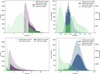 |
Fig. 1 Histograms of the redshift (top panel) and S/N (bottom panel) for quasars (left column in purple for the WEAVE mock catalog and in green for DESI EDR) and galaxies (right panel in blue for the VIPERS and in green for DESI EDR). The unfilled histograms show the distributions of the parent samples, while the filled histograms show the distributions of the final samples after all the data selections. |
2.2 VIPERS galaxy catalog
The main goal of this analysis is to compare the performance of various ML techniques in predicting the continuum of quasars. As part of this study, we test the ability of the selected algorithms to predict different spectral shapes, including those of galaxies. For this, we apply the same methodology used on quasars also on galaxy spectra. To compile a galaxy sample, we use the catalog from the VIMOS Public Extragalactic Redshift Survey (VIPERS; Guzzo & VIPERS Team 2013; Garilli et al. 2014; Scodeggio et al. 2018) that is a spectroscopic survey completed with the VIMOS spectrograph (Le Fèvre et al. 2003). Its primary purpose was to measure the redshift of almost 105 galaxies in the 0.5 < z < 1.2 range. The area covered by VIPERS is about 25.5 deg2 on the sky. Only galaxies brighter than iAB = 22.5 were observed, relying on a preselection in the (u - g) and (r - i) colorcolor plane to remove galaxies at lower redshifts (see Guzzo et al. 2014 for a more detailed description). The Canada-France-Hawaii Telescope Legacy Survey Wide (CFHTLS-Wide; Mellier et al. 2008) W1 and W4 equatorial fields compose the galaxy sample, at RA ≃ 2 and ≃22 hours, respectively. The VIPERS spectral resolution (R ~ 250) allows us to study individual spectroscopic properties of galaxies with an observed wavelength coverage of 5500-9500 Å. The data reduction pipeline and the redshift quality system are described in Garilli et al. (2014). The final data release provides reliable spectroscopic measurements and photometric properties for 86 775 galaxies (Scodeggio et al. 2018).
Starting from the VIPERS Public Data Release-2 (PDR2) spectroscopic catalog, we limit our sample to galaxies with a redshift confidence level of 99% (3.0 ≤ zflag ≤ 4.5), reducing the redshift interval of the catalog within the range 0.4 < z < 1.2 (see Fig. 1 for the redshift and S/N distributions). This selection reduces the sample to ~50000 sources, including narrow-line AGNs, star-forming galaxies, and passive galaxies. The selection on the redshift confidence level interval has the side effect of shifting the distribution in S/N toward higher values. Galaxies with the chosen interval of zflag show apparent spectral features in the spectrum used to measure the redshift. The second selection is in the redshift range, limited to 0.5 ≤ z ≤ 0.75 to have the entire rest frame wavelength range of interest 3500-5500 Å covered in the data. These selections reduce the sample size to the ~30 000 observed galaxy spectra.
Having a good measurement of the true continuum as a label during the training of the NN model is essential. We estimate the continuum of the VIPERS galaxy spectra by modeling them (as done in Pistis et al. 2024) using the penalized pixel fitting code (pPXF; Cappellari & Emsellem 2004; Cappellari 2017, 2023), which makes it possible to fit both the stellar and gas components via full-spectrum fitting. After shifting the observed spectra to the rest frame and masking out the emission lines, the stellar component of the spectra is fitted with a linear combination of stellar templates from the MILES library (Vazdekis et al. 2010) convolved to the same spectral resolution as the observations. The gas component is fitted with a single Gaussian for each emission line.
2.3 DESI quasar and galaxy catalogs
While the WEAVE mock and VIPERS catalogs are used to train and test the NN models, we also studied how these models can be deployed on unseen datasets with similar properties. For this step, we chose the Early Data Release1 (EDR) of the Dark Energy Spectroscopic Instrument (DESI; DESI Collaboration 2022, 2024) which is the largest spectroscopic survey to date with characteristics similar to those expected for WEAVE, such as the spectroscopic resolution (between 2000 and 5000 at different wavelength intervals) and the redshift range of the observed targets. Galaxies in DESI/EDR also share redshifts similar to those of the VIPERS sample. For quasars, we removed the broad absorption line (BAL) quasars. The BALs are removed because the mock catalog at present does not include these sources and their presence would lead to a more complex assessment of the generalization performance without having a close look at these specific cases. For this task, we use the public value added cata-log2 (VAC) by Filbert et al. (2024). The VAC catalog contains the absorption indices (AI, defined by Hall et al. 2002) for the metal lines CIV and SiIV. We considered a BAL any quasar with an AI value higher than 0 for any metal line. For both quasars and galaxies, we selected sources with redshift ranges that cover the same interval as the WEAVE mock and VIPERS catalogs. The DESI catalogs are reduced to 9000 quasars and 100 000 galaxies (see Fig. 1 for the redshift and S/N distributions).
The public DESI EDR catalog contains the continua of both quasars and galaxies computed with Redrock, which is intended as a redshift fitter and classifier. Redrock fits PCA templates of three broad, independent classes of objects: stars, galaxies, and quasars. The spectra are classified according to their minimum χ2 of the fit. In the following, we compare our results against the available Redrock continuum, which is independent of what is obtained through NNs. However, the DESI pipeline has been expanded, for example, with QuasarNET (Busca & Balland 2021) for quasars and SPENDER (Melchior et al. 2023; Liang et al. 2023a,b) for galaxies, which provide NN-based high-quality continua for DESI sources.
Before proceeding with our work, we verify that DESI and the WEAVE mock quasars share broadly similar continuum shapes. For this, we compared the distribution of the flux ratio FR, defined as FR = F (λ = 1450 Å)/F (λ = 1800° Å), and the slope m, defined as ΔF/Δλ with Δλ = 1800-1450 Å. This comparison is shown in Fig. 2. WEAVE mocks generally overlap with the DESI data for the R parameter, while displaying a slope distribution shifted toward lower values. As we show in the following sections, the best models trained on WEAVE data generalize sufficiently well and can be applied to DESI data with satisfactory success.
Finally, we employ the DESI sample to test our NN’s performance in recovering physical quantities. For the quasar case, we estimate the evolution of the mean optical depth (see Sect. 5 for details) and compare with previous results (Becker et al. 2013; Turner et al. 2024). For the galaxy case, we compute the D4000n break and compare the results between the NNs and Redrock3, released with the DESI EDR. We did not compute the underlying continua for the DESI spectra with other traditional methods, such as pPXF, used for VIPERS.
3 Machine learning approach and architectures
We focus first on the reconstruction of the continuum for quasar spectra (see Sect. 4), and then we test how well the same architecture performs in modeling the stellar component in galaxy spectra after a retraining and optimization step (see Sect. 7). For this reason, quasars and galaxies are treated separately, and each NN is optimized and trained independently between quasars and galaxies. In this work, we used three different classes of NNs: autoencoders, CNNs, and U-Net. Figure 3 shows the flow chart of the methodology followed in this work. The raw spectra are preprocessed (see Sect. 3.2 for details) to produce similar spectra (in wavelength and flux ranges) to pass as input to the NNs. These architectures are then optimized by randomly searching the hyperparameters (e.g., the number and size of layers or kernels). The optimization is performed with a random search for autoencoders for 100 trials. The CNNs and U-Net are optimized with a Bayesian search for 50 trials. After optimizing each architecture, we selected the best model to predict the continua of the spectra. The performances of each NN are then compared (see Sect. 4 for details) via the absolute fractional flux error (AFFE) metric and bias in the prediction when found. The best architecture is finally tested on the physical aspect (see Sect. 5 for details).
During the training phase, we adopted a general strategy shared among all NNs. We randomly divided the samples into training (50% of the total sample), validation (25% of the total sample), and test (25% of the total sample). At each training cycle, the order of the training spectra is randomly shuffled. We adopt an early stopping strategy (Prechelt 2012) if there are no updates on the loss for the validation sample during the training process for five consecutive epochs. We chose a loss defined by the mean squared error between the true and predicted continua. Because the analysis is performed in the source’s rest frame, not all spectra cover the whole wavelength range. A few pixels can be missing at the edges of the spectra. For this reason, we assign the value 0 to the missing parts at the edges of the spectra, adding a masking layer to the autoencoder to exclude this portion of the spectra.
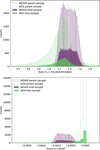 |
Fig. 2 Histograms of the ratio (top) and slope (bottom) of the quasar spectra between the rest frame wavelengths λ = 1800 Å and λ = 1450 Å for the WEAVE mock catalog (purple) and the DESI EDR (green). The unfilled histograms show the distributions of the parent samples, while the filled histograms show the distributions of the final samples after all the data selections. |
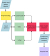 |
Fig. 3 Graphical representation of the workflow. The dotted double arrows represent recursive steps. |
3.1 Performance metrics
To measure the quality of the fit, we use the AFFE as a fit-goodness metric (see, for example, Liu & Bordoloi 2021; Turner et al. 2024). The AFFE is defined as
 (1)
(1)
where Fpred is the predicted output and Ftrue is the true continuum of the simulated quasar spectra or the pPXF fit of the stellar component for the galaxy spectra. To check the presence of bias as a function of the wavelength, we use the fractional flux error (FFE) defined as:
 (2)
(2)
3.2 Data preprocessing
Data preprocessing is a critical step in many ML applications. This study follows a similar preprocessing used in Turner et al. (2024). The first step in predicting the continuum is to sample the spectra on the same grid in the same rest frame range. We interpolated the simulated quasar spectra in the range 1020-2000 Å within pixels of 0.2 Å width, while we interpolated the observed galaxy spectra in the NUV-optical range 3500-5500 Å within pixels of 1 Å width. The difference is due to the disparity in spectral resolution between the WEAVE and VIPERS surveys.
The second step is to scale all the data to the same range to avoid the specific features of some spectra dominating over others. Each quasar spectrum, both in the WEAVE and the DESI samples, is normalized by the median flux at λ = 1450 Å within a window of Δλ = 50 Å. The galaxy spectra, instead, are normalized according to the median flux over the whole wavelength range, as was done in the analysis with pPXF.
3.3 Autoencoders
The first architecture we consider in our study is the autoencoder. They consist of an encoder and a decoder, where the encoder maps the input data into a lower-dimensional latent space, and the decoder attempts to reconstruct the original input from this compressed representation. By minimizing the difference between the original data and its reconstruction, autoencoders learn to capture the most essential features of the input. Our application relies on a general architecture where the encoder and decoder consist of three layers plus a layer with a bottleneck function. This is motivated by the intelligent quasar continuum neural network (iQNet; Liu & Bordoloi 2021), which we take as a starting point. Further updates are performed to adapt the original IQNet for our specific problem, and the models we used for the different data are reported in Table D.1 in the Appendix D.
We also compare the modified architecture with the direct application of the original IQNet model, without any particular change except for the preprocessing of the data. Specifically, normalizing the spectra by flux at λ = 1450 Å instead of the min-max scaling used by Liu & Bordoloi (2021) required us to change the loss function from binary cross-entropy (Liu & Bordoloi 2021) to mean squared error.
3.4 Convolutional neural networks
We further explore the performance of a CNN starting from the Lyα Continuum Analysis Network (LyCAN; Turner et al. 2024), which was designed to handle DESI spectra and which we use as a reference. A CNN is a regularized type of feedforward NN that learns features by itself via the application of a kernel or filter (LeCun et al. 2015). The kernel moves along the spectra with a given step, called a stride, performing an element-wise multiplication operation between the kernel and the input. After each convolutional layer, a CNN has a pooling layer with the goal of reducing the size of the convolved feature. The pooling layer can be of mainly two types: (i) max-pooling, where the max value within the kernel is taken; and (ii) average-pooling, where the average of all values within the kernel is taken.
We built our CNN by optimizing the architecture and the hyperparameters on both the WEAVE mocks and VIPERS observed spectra. Table D.2 in Appendix D summarizes the updated CNN architectures for both WEAVE and VIPERS data.
3.5 U-Net
The U-Net is a deep learning model initially designed for biomedical image segmentation (Ronneberger et al. 2015; Zhang et al. 2018; Li et al. 2024), which is effective and versatile. Unlike traditional CNNs that struggle with pixel-level predictions, U-Net excels by leveraging a unique encoder-decoder structure that captures context and fine details simultaneously. The architecture’s encoder reduces the input image’s spatial dimensions through a series of convolutional and max-pooling layers. In this process, the model learns complex features and hierarchical representations. Instead, the decoder reconstructs the spatial dimensions using transposed convolutions and concatenations, combining them with the encoder’s corresponding feature maps. A key aspect of U-Net is its skip connections, which directly link the corresponding encoder and decoder layers. These connections ensure that high-resolution features are preserved and propagated through the network, enhancing the model’s ability to produce detailed and accurate segmentations. Table D.3, in Appendix D, reports the specific characteristics of the architectures we developed for the different data used in this work.
4 Application to the spectra
In this section, we describe the application of the NNs to the quasars. We start our analysis by considering the performance of the autoencoders, moving next to the analysis of the CNNs and U-Nets.
We give as input to the two autoencoders (the original IQNet and our bespoke model) the red part of the quasar spectra (1216 Å < λ < 2000 Å in the rest frame) and predict the continuum in the entire spectrum range (1020 Å < λ < 2000 Å in the rest frame), as was done in Liu & Bordoloi (2021) and Turner et al. (2024). The red part of the quasar spectra is generally more regular than the blue side at these high redshifts because the red part is less contaminated by absorption lines that give rise to a thick forest that blankets the quasar continuum. However, as an additional test, we examine whether passing the entire spectrum during training would improve the goodness of fit in the Lyα forest region.
The performances of autoencoders are shown in Fig. 4 (top panels). Each histogram reports the AFFE metric for the quasar continuum fit using the original iQNet and our bespoke autoencoder, training both on the full spectrum and on the red part. In the three panels, we show instead the AFFE for the whole spectrum and in the red (λ > = 1216 Å) and blue (λ < 1216 Å) parts, separately. Although the performance of iQNet is already satisfactory (<1% deviations), our tailored architectures find a median AFFE consistently lower than iQNet’s. The iQNet architecture also shows a more widespread distribution than our tweaked architectures. Figure 5 shows an example fit of a quasar spectrum. Appendix E contains more examples of fit performed with the autoencoders.
The AFFE provides a global metric for the performance of the architectures. Instead, to examine whether any systematic bias arises as a function of wavelength, we study the performance on selected parts of the spectrum, considering the FFE as a function of wavelength (Fig. 6). We found an FFE almost constant in all cases. The overall small scatter, especially for the case of the tailored autoencoder, makes the application of this method reasonable to most problems where low-amplitude biases are not critical. However, once the FFE is looked at over the whole wavelength range, iQNet shows a bias (negative slope), making the bespoke architecture preferable given the fluxes are consistent with zero over an extensive range of wavelengths for λ ≥ 1216 Å. The negative slope persists even though the training and test samples are shuffled. This suggests that iQNet requires a larger sample to reduce the bias. Moreover, we did not find strong biases in the performances of the autoencoders with the S/N of the spectra or the redshift of the source (see Appendix C for the details).
We next move to the analysis of the performance of the NNs, testing against each other the U-Net and CNN architecture, also in comparison with the results of the LyCAN architecture (Turner et al. 2024). Examining the AFFE distribution (Fig. 4), the U-Net performs slightly worse than the CNN and LyCAN, especially in the region of the Lyα forest. However, the performance over the entire spectrum is comparable among U-Net and LyCAN, with a difference of a maximum of 0.2 percent while the CNNs have performances equal to the autoencoders (top panels of Fig. 4). Figure 5 shows an example fit of a quasar spectrum. More examples of fits performed with these architectures are shown in Appendix E.
We again examined possible biases in the continuum reconstruction in particular parts of the spectrum and studied the FFE as a function of the wavelength (Fig. 6). We found an FFE mainly constant in these cases. The LyCAN shows a small bias, with a positive slope. The U-Net appears instead less prone to biases locally, although there are more fluctuations in the FFE compared to the other CNNs. As already noted when studying the AFFE, the autoencoder also performs better in this metric.
Checking for biases in the performance, we found a strong bias of the AFFE for the U-Net with the S/N, where better quality spectra have better-predicted continua.
We conclude that both autoencoders and CNNs perform well in reconstructing the quasar continuum, with the former showing better precision, accuracy, and stability. The reduced computational time and effort of the autoencoders (≈ 10 times lower than CNNs and U-Nets) is another aspect in favor of this class of NNs.
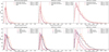 |
Fig. 4 Performance of NN predictions: histograms of the absolute fractional flux error (AFFE) for the autoencoders (top row) and CNN plus U-Net (bottom row) applied to the quasar datasets. The vertical lines show the median AFFE value for each histogram. |
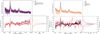 |
Fig. 5 Example quasar spectrum. The top panel of each plot shows the data, the true continuum, and the fits of different runs of the autoencoders (left) and CNNs (right). The bottom panel shows the FFE as a function of the rest frame wavelength for different runs of the autoencoders and their distributions. |
5 Astrophysical tests and generalization
Having compared the performance of various NNs on the datasets that have been used for training, we explore further the ability of these architectures to be deployed on similar yet nonidentical datasets without any training or new optimization. This section addresses how well these methods can be generalized to new datasets. Specifically, we consider a quasar sample from DESI onto which we deploy the NNs. Following continuum normalization using the best-performing NNs, we extract physical information on the mean transmitted flux for the Lyα forest in quasars which we compare to the measurements from the literature.
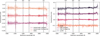 |
Fig. 6 Performance of NN predictions with wavelength: Median fractional flux error (FFE) as a function of the wavelength for the autoencoders (left panel) and CNN (right panel). The shaded area shows the 16th and 84th percentiles of the distribution of the whole sample. The vertical shift is introduced to improve visualization. The black dotted lines show the zero point of each run. The shaded black vertical lines show the positions of the main emission lines in the wavelength range. |
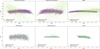 |
Fig. 7 Distribution of the spectra in the latent spaces of the autoencoders (upper row) and CNNs (bottom row) for the WEAVE training sample (purple) and the DESI final sample (green). |
5.1 Testing covariate shift
When considering the application of NNs trained on different datasets, we should closely examine the impact of the covariate shift problem (Sànchez et al. 2014; Hoyle et al. 2015; Rau et al. 2015; Zitlau et al. 2016). A covariate shift occurs when the input distribution changes between training and testing samples, causing the model to perform poorly on new data. This shift can lead to mismatches between learned representations and actual test distributions.
We consider the minimal representation of the input data (training sample of WEAVE mocks and DESI data; Ambrosch et al. 2023; Ginolfi et al. 2025; Belfiore et al. 2025) from each NN, corresponding to the central layer for the autoencoders and the dense layer with the lowest dimension for the CNNs. Then, we perform PCA on WEAVE data, and we apply the same transformation to both samples. The PCA representation of the data is then plotted in a 2D space (the first component has ~90% of variance for all cases, see Fig. 7) for all NNs. We observe that the DESI sample explores a wider portion of the latent space for the autoencoders with respect to the WEAVE training sample. CNNs, instead, can map both samples in a more similar latent space. We choose to use the linear transformation given by the PCA because it allows us to be consistent in the comparison of the two samples. Non-linear transformations, such as uniform manifold approximation and projection (UMAP) or t-distributed stochastic neighbor embedding (t-SNE), would break the consistency between samples by their nature, leading to a more difficult comparison of the latent spaces.
To study the effects of training in a subregion of the latent space and then applying the model to a sample that occupies a separate subregion, we split the 2D representation of the training sample into two parts at PCA = 0: vertically (left and right) and horizontally (bottom and top). By doing this, we reduce the sample size for the training by half and predict the continuum on spectra that are not close to those used for the training. Splitting both vertically and horizontally is useful for breaking the symmetries in the distributions of the spectra in the latent space.
After splitting the 2D representation of the training sample, we retrain each NN again on the left and test it on the right, and vice versa. Similarly, we repeat the same procedure for the horizontal splitting. Despite the presence of predominant vertical symmetry, we do not observe strong biases in the distributions, with most of the AFFE values below ≈0.02-0.03 for the autoencoders. However, in some cases, we observe an excess at the tail of the AFFE distributions for high values that remain nevertheless below ≈0.05-0.06 while the CNN vertically split reach values of 0.10. Even in the most pessimistic case, where the NNs have been trained only on half the latent space, the performances decrease by a factor ≈2 or 3 for some cases with the predicted continua, with an AFFE associated with ≈2.5 percent when an excess in the distribution is observed.
From this exercise, we conclude that the NNs included in this work can also be successfully deployed on different datasets than the one employed during training. As a last exercise, we apply the best-performing NNs to two astrophysical problems that rely on a precise and accurate reconstruction of the continuum level in quasars and galaxies, using the DESI EDR sample.
We estimate the mean transmitted flux in the Lyα region (Sect. 5.2). We performed the test with the continua estimated with our optimized autoencoder, which consistently displays good performance metrics.
5.2 Optical depth of the Lyα forest
For a more physical test of quasar continua, we estimated the mean transmitted flux, converted as optical depth τ, in the region of the Lyα forest, assuming the continua derived by the autoencoder. The weights obtained during the training phase with the WEAVE mock spectra are directly applied to the DESI EDR catalog without any new training to estimate the continua of the spectra. We then take the portion of the spectra in the rest frame wavelength range 1070 Å-1160 Å to avoid contamination from the Lyα and OVI (Kamble et al. 2020). At each pixel of the spectra in this range, we associated a redshift zLyα of the absorber given by the equation:
 (3)
(3)
In each zLyα bin (binwidth of 0.1), we computed the mean transmission defined as
 (4)
(4)
where Fobs is the observed flux and Fcont is the estimated continuum at the corresponding zLyα. Finally, we computed the median transmitted flux 〈f〉 and converted it to optical depth τ = − ln〈f〉. We emphasize that this analysis aims to test whether we can recover previous estimates of this quantity and not present a novel measurement of the IGM mean optical depth. As such, we report the raw quantity derived as defined above, referring the readers to detailed literature on the subject for accurate measurements (Aguirre et al. 2002; Schaye et al. 2003; Becker et al. 2013; Turner et al. 2024). We also did not apply any correction for optically thick absorbers (Becker et al. 2013) or metals (Schaye et al. 2003; Kirkman et al. 2005; Faucher-Giguère et al. 2008).
Figure 8 shows the evolution of our measurement of the optical depth. Our simple approach can reproduce quite well the observed evolution in more bespoke studies (Becker et al. 2013; Turner et al. 2024), which implies a good degree of prediction of the quasar continuum in unseen DESI data. For comparison, we reported in the same figure the tabulated values in Turner et al. (2024) (Table 3, final values, bias-corrected measurements corrected for metal line absorption according to Schaye et al. 2003 and optically thick absorbers according to Becker et al. 2013) and the best-fit relationship of Becker et al. (2013). The autoencoder thus demonstrates an excellent degree of generalization, so that it can be trained on mock spectra and applied without further tuning to comparable but not identical data.
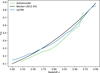 |
Fig. 8 Redshift evolution of the effective optical depth (τeff) observed in the DESI EDR sample. We report the values obtained in this study with the continua estimated with the optimized autoencoder (green). The evolution found by Becker et al. (2013) (black) and the results on the DESI observation done with LyCAN (Turner et al. 2024) (blue) are also shown. |
6 A note on computational efficiency
The above analysis demonstrates that the autoencoder provides a lightweight yet powerful alternative to more complex architectures when determining the continuum of quasars. An added benefit of this simplicity is that the autoencoder is much less computationally expensive than the U-Net and CNNs, by a factor of ~20 in computational time, resulting in a better choice when analyzing a large data sample is necessary. The difference in performance of 0.2% between the autoencoder and the CNN is negligible with respect to the difference in computational time, especially when optimization and training steps must be performed.
Figure 9 visualizes the training and prediction times for all NNs using three NVIDIA A2 GPUs. The training and prediction phases are performed using the TensorFlow mirrored strategy to distribute the work between the three GPUs. For a fair comparison, the batch size is set to 256 spectra (limited by avoiding memory problems with the U-Net and CNNs) for all NNs, but, in principle, the batch size for autoencoders can be easily increased, reducing even further the computational time. The main difference is found in the training time, where U-Net and CNN have an order of magnitude longer time. This is even more visible during the optimization of the hyperparameters, when the autoencoders can perform 100 trials in a fraction of the time needed for 50 trials for the U-Net and CNNs. Moreover, the computational time does not increase linearly with the sample size. Assuming a sample size of 1 000 000 spectra to fit, an autoencoder would spend about 3 minutes, while a CNN would spend about 40 minutes.
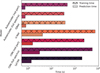 |
Fig. 9 Visualization of the training and prediction times for the autoencoders, U-Net, and CNNs. |
7 Test on galaxies
Having investigated the performance of each NN on quasars, we move to the question of whether these architectures can be generalized to different continuum shapes with minimal modifications (i.e., new optimization and training steps). Bespoke NNs tailored for the analysis of galaxy spectra can be found in the literature, for example, SPENDER (Melchior et al. 2023; Liang et al. 2023a,b). Applications with a focus on galaxies should therefore turn to these dedicated networks. This section aims solely at testing the performance of NNs developed for quasars when applied (nearly) out-of-the-box on galaxy spectra.
We thus focused our attention on the performance of each architecture in predicting the shape of galaxy spectra from the VIPERS survey. Compared to a mostly featureless power-law continuum plus emission lines, galaxies present a richer set of features encoded in their stellar continuum. Without heavily restructuring the algorithms, the architectures used for the quasars undergo a new optimization step and re-training using a sub-sample of VIPERS spectra. In this way, we check the performance of the NNs with a limited tuning of the methodology. We give as input to the NNs the whole galaxy spectra (3500 Å < λ < 5500 Å in the rest frame) and predicted the continuum in the same range. We selected galaxies within a redshift range of 0.5 ≤ z ≤ 0.75 to have the observations within the whole wavelength range. No particular additional data selection (e.g., a threshold on the S/N values of the spectra) was applied to the training sample.
Figure 10 shows the AFFE distributions for the NNs applied to galaxy spectra. As in the quasar case, the autoencoder and CNN perform better than the U-Net for the fit of the continua, with an AFFE of ≈1% with respect to the continua estimated using traditional methodology such as pPXF (Cappellari & Emsellem 2004; Cappellari 2017, 2023). The same methodology used for the quasars can be applied to galaxies with an increased median AFFE of ≈0.5%.
Also, for galaxies, we tested the ability of our autoencoder to make reliable predictions on unseen DESI galaxy spectra. Fig. 11 shows the comparison of the values for the D4000n break calculated over the continua predicted by the autoencoder and the continua estimated using pPXF for VIPERS and Redrock for DESI. We stress again that the use of the continua made with Redrock is dictated by its availability in the DESI EDR catalogs, and bespoke algorithms within the full DESI pipeline will outperform this algorithm in continuum determination. Still, its use is sufficient to reach our main conclusion on the generalization capability of the NNs explored in this study.
We found a value of the Pearson correlation coefficient of 0.94 and 0.92 for VIPERS and DESI, respectively, between the D4000n break calculated over the continua predicted by the NN and the reference continua (estimated with pPXF for VIPERS and Redrock model for DESI). In the Bland-Altman plot (Bland & Altman 1986), both datasets show a small shift (bias) of the means from 0; however, for both VIPERS and DESI cases, the data show a hint of a negative slope. For these datasets, the bias is proportional to the measurements. We thus conclude that also for the galaxy spectra, the autoencoder generalizes sufficiently well to unseen data, and it is suitable for astrophysical problems.
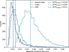 |
Fig. 10 Performance of NN predictions: Histograms of the absolute fractional flux error (AFFE) for NNs applied to VIPERS galaxies for the novel architectures used in this work. |
8 Summary
This study has focused on a comparative analysis of the performance of various NNs to predict the continuum of quasars. Specifically, we compared the performance of an autoencoder, a CNN, and a U-Net with two published architectures (iQNet from Liu & Bordoloi 2021 and LyCAN from Turner et al. 2024). Initial comparison was performed on a large catalog of mock spectra for the WEAVE survey (Jin et al. 2024). Using the DESI EDR quasar catalog (DESI Collaboration 2022, 2024), we further tested the ability of these architectures to generalize to unseen datasets without the need of retraining. Moreover, with minor optimizations, we studied to what extent NNs tailored to handle quasar spectra can also be deployed on more complex spectral shapes, such as galaxies. For this task, we rely on galaxies observed with the VIPERS survey (Garilli et al. 2014; Scodeggio et al. 2018; Vergani et al. 2018; Vietri et al. 2022; Figueira et al. 2022; Pistis et al. 2022, 2024) and on the DESI EDR galaxy catalogs. Fig. 12 summarizes the performances of the various architectures applied to the quasar problem, using the AFFE distributions as a metric.
The optimized autoencoder developed in this work improves the width of the AFFE distribution when applied to z ≳ 2 quasars with respect to the original iQNet by Liu & Bordoloi (2021) and reaches better performances than those of Turner et al. (2024) with LyCAN (see Sect. 4). The autoencoder also performs well with galaxy spectra after a retraining and optimization step, but without restructuring the architecture (see Fig. 10 for both passive and active sources). While custom NNs tailored to the galaxy problem can be found in the literature, this test shows a good versability of the architectures explored in this work to a variety of continuum shapes.
Finally, we directly applied the autoencoder to the DESI EDR data (see Sect. 5) without retraining, for both the quasar and the galaxy case. With the predicted continua, we estimated the evolution of the mean transmitted flux in the Lyα forest region converted to optical depth. We found an evolution in agreement with previous studies (Becker et al. 2013; Turner et al. 2024) indicative of the possibility of using these NNs in previously unseen datasets from different surveys. Likewise, for galaxies, we estimated the D4000n break with the continua estimated with the autoencoder for both VIPERS and DESI galaxy catalogs and compared them with the values of the continua estimated with pPXF for VIPERS and the model, done with Redrock, released with the DESI EDR catalog. In both cases, the linear fit is close to the y = x line, with a deviation around D4000n = 0.2.
The main conclusions can be summarized as follows:
The autoencoder performs as well as more complex architectures for much lower computational costs;
The autoencoder performs well with both quasar and galaxy spectra;
The direct application to DESI EDR data confirms the generalization of the method to unseen datasets, which are similar but not identical to the training data;
All the architectures tested in this work show a small bias of the FFE with the wavelength related to the magnitude selection of the sample (see Appendix A), and high-precision tasks should identify suitable metrics for assessing the impact of these offsets.
A simple autoencoder proves useful for reaching good precision (median error of ≈1%) in the continuum predictions while limiting computational resources in analyzing large data samples. This NN can become a versitile tool for studies on absorbers in the quasar spectrum, for example tracking the evolution of strong absorbers in the CGM, such as CIV (e.g., Cooksey et al. 2013; Davies et al. 2023a,b), SiIV (e.g., D’Odorico et al. 2022), and MgII (e.g., Matejek & Simcoe 2012; Chen et al. 2017; Zou et al. 2021) or the auto- and cross-correlation of Lyα absorbers (e.g., du Mas des Bourboux et al. 2020).
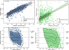 |
Fig. 11 Comparison of the D4000n values estimated with the NN in this work and with pPXF (Pistis et al. 2024) (left panel) for VIPERS (in blue) and with Redrock (right panel) for DESI (in green). The red solid line shows the line y = x, the light-shaded area limited by dashed lines shows 95% prediction limits, and the dark-shaded area shows the 95% confidence limits. The density plots show the one-, two-, and three-sigma levels of the 2D distributions. Top panel: Direct comparison of the two methods. Bottom panel: Bland-Altman plot. |
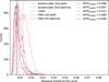 |
Fig. 12 Performance of NN predictions: Histograms of the absolute fractional flux error (AFFE) for NNs applied to the WEAVE mock catalog for the novel architectures used in this work. |
Data availability
Supplementary materials with the trained models for all architectures and both quasar and galaxies are available on Zenodo, at https://zenodo.org/records/15011824.
Acknowledgements
We thank the referee for insightful comments that have improved the content and presentation of this work. F. Pistis, M. Fumagalli, and M. Fossati have been supported by the European Union - Next Generation EU, Mission 4, Component 1 CUP H53D23011030001. W. J. Pearson has been supported by the Polish National Science Center project UMO-2023/51/D/ST9/00147. A. Pollo has been supported by the Polish National Science Centre grant 2023/50/A/ST9/00579. This paper uses data from the VIMOS Public Extragalactic Redshift Survey (VIPERS). VIPERS has been performed using the ESO Very Large Telescope, under the “Large Programme” 182.A-0886. The participating institutions and funding agencies are listed at http://vipers.inaf.it. This research used data obtained with the Dark Energy Spectroscopic Instrument (DESI). DESI construction and operations are managed by the Lawrence Berkeley National Laboratory. This material is based upon work supported by the U.S. Department of Energy, Office of Science, Office of High-Energy Physics, under Contract No. DE-AC02-05CH11231, and by the National Energy Research Scientific Computing Center, a DOE Office of Science User Facility under the same contract. Additional support for DESI was provided by the U.S. National Science Foundation (NSF), Division of Astronomical Sciences under Contract No. AST-0950945 to the NSF’s National Optical-Infrared Astronomy Research Laboratory; the Science and Technology Facilities Council of the United Kingdom; the Gordon and Betty Moore Foundation; the Heising-Simons Foundation; the French Alternative Energies and Atomic Energy Commission (CEA); the National Council of Science and Technology of Mexico (CONA-CYT); the Ministry of Science and Innovation of Spain (MICINN), and by the DESI Member Institutions: www.desi.lbl.gov/collaborating-institutions. The DESI collaboration is honored to be permitted to conduct scientific research on Iolkam Du’ag (Kitt Peak), a mountain with particular significance to the Tohono O’odham Nation. Any opinions, findings, and conclusions or recommendations expressed in this material are those of the author(s) and do not necessarily reflect the views of the U.S. National Science Foundation, the U.S. Department of Energy, or any of the listed funding agencies.
Appendix A Bias on the fractional flux error
Fig. A.1 (top panel) shows the FFE as a function of the rest frame wavelength for the cases of passing the red part of the spectra or the whole spectra as input to the autoencoder and iQNet. Different colors correspond to different r-band magnitude cuts of the sample. In all cases, using less restrictive cuts improves the overall performance of the autoencoders. iQNet seems to be more sensitive to magnitude selection. We have applied a cut at r < 21 to minimize the bias while maximizing the sample statistics through our analysis.
Fig. A.1 (bottom panel) shows the FFE as a function of the res-frame wavelength for the case of U-Net, optimized CNNs and LyCAN. Only the restrictive cut, such as r < 19.5, reduces CNN performance. Performance in the Ly-α forest region improves with less restrictive cuts. LyCAN is less sensitive to the magnitude bias, except in the Ly-α forest region
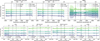 |
Fig. A.1 Fractional flux error as function of the rest frame wavelength for the autoencoders (top panels) and the CNNs (bottom panels) for different selections on the r-band magnitude. |
Appendix B Effects of S/N selection
A relevant question in the training step is what S/N threshold should be imposed. Specifically, we want to understand whether the algorithm performs better when seeing high-quality data or if we should feed as much information as possible, presenting low-S/N spectra in the training step. To this end, before creating our training and test samples, we removed sources with a median S/N value of the spectra lower than a given threshold. These sources are then added directly to the test sample to check the performance in generalizing low-S/N data starting from high-S/N data. Fig. B.1 (left panel) shows the results of this analysis. For iQNet, we see hints of a break at S/N > 2, though when considering error bars, the median AFE appears to be roughly constant. We conclude that the autoencoders can generalize the fit of high-S/N spectra for low-S/N spectra. The iQNet can learn better from a larger dataset, including spectra at low S/N. The analyses in this study are done without selecting the samples on the S/N.
We follow the same approach for the CNNs. Fig. B.1 (right panel) shows the results of this analysis. For the U-Net and CNNs, the median AFFE and its scatter increase with the S/N threshold. The deviation is more evident for the CNN trained on the whole spectrum and LyCAN. Thus, for all architectures, we conclude that training in larger, more comprehensive datasets is more useful than training in high-quality samples.
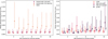 |
Fig. B.1 Median AFFE as a function of the selection S/N-threshold for the autoencoders (left) and the CNNs and U-Net (right panel) for quasars. The error bars show the 16th and 84th percentiles of the AFFE distribution in each run. The horizontal shift between points is introduced to improve the visualization. |
Appendix C Model biases
As a final performance metric, we consider the dependence of the fit quality as a function of the S/N of each spectrum and redshift of each quasar. Fig. C.1 shows the median relation between AFFE (left panel) and FFE (right panel) versus S/N and redshift. For the AFFE, the median relation is almost constant in the whole S/N and redshift ranges, with a rise only for z > 3.8. The shift from the median in the last redshift bin is primarily due to the reduced statistics in that bin. The iQNet architecture shows a more widespread scatter around the full sample median. The situation is similar for the FFE, with the most shifted bin being the last redshift bin and the overall median relation constant. The iQNet architecture again shows a more widespread scatter.
As for the autoencoders, we checked the dependence of the quality of the fit on the S/N and redshift of each source, also for the CNNs (Fig. C.1). U-Net, the CNN trained on the red part only, and LyCAN show a decreasing AFFE with the S/N, a trend that is more evident in the case of the U-Net, where the median relation drops below the full sample median. The AFFE, instead, increases with the redshift, monotonically for the U-Net, especially above z = 3.5, while it is generally constant for the other architectures, except for the highest redshift. Regarding the FFE, all architectures show a systematic shift in both S/N and redshift. Only the U-Net underestimates the continuum at every S/N and redshift. In contrast, CNNs and LyCAN tend to overestimate the continuum.
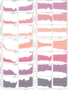 |
Fig. C.1 Systematic biases of autoencoders (top row) and CNN plus U-Net (bottom row) for galaxies. The left (right) column shows the AFFE (FFE) as functions of S/N and z. The dotted lines show the median AFFE values and the zero point for the FFE. The shaded region shows the 16th and 84th percentiles. |
Appendix D Summary of architectures
Tables D.1, D.2, and D.3 summarizes the optimized architectures used in this work. The sizes of each layer and additional information, such as activation functions and kernel sizes (for convolutional layers), are explicitly reported in the tables.
Architecture of the optimized autoencoders applied to WEAVE (red and full spectra) and VIPERS data.
Architecture of the optimized CNNs applied to WEAVE (red and full spectra) and VIPERS data.
Architecture of the optimized U-Nets applied to WEAVE and VIPERS data.
Appendix E Fit example: Autoencoders and CNNs
Fig. E.1 shows examples of spectra for the case of giving to the optimized autoencoder only the red part of the spectra or the whole spectra as input and iQNet.
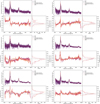 |
Fig. E.1 Example spectra of quasars. The top panel of each plot shows the data, the true continuum, and the fits of different runs of the autoencoders. The bottom panel shows the FFE as a function of the rest frame wavelength for different runs of the autoencoders and their distributions. |
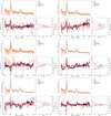 |
Fig. E.2 Example spectra of quasars. The top panel of each plot shows the data, the true continuum, and the fits of different runs of the CNNs. The bottom panel shows the FFE as a function of the rest frame wavelength for different runs of the autoencoders and their distributions. The shown spectra are the same as Fig. E.1. |
References
- Abazajian, K. N., Adelman-McCarthy, J. K., Agüeros, M. A., et al. 2009, ApJS, 182, 543 [Google Scholar]
- Abraham, V., Deville, J., & Kinariwala, G. 2024, RNAAS, 8, 46 [Google Scholar]
- Aguirre, A., Schaye, J., & Theuns, T. 2002, ApJ, 576, 1 [Google Scholar]
- Ambrosch, M., Guiglion, G., Mikolaitis, S., et al. 2023, A&A, 672, A46 [NASA ADS] [CrossRef] [EDP Sciences] [Google Scholar]
- Angthopo, J., Granett, B. R., La Barbera, F., et al. 2024, A&A, 690, A198 [NASA ADS] [CrossRef] [EDP Sciences] [Google Scholar]
- Bahcall, J. N., & Goldsmith, S. 1971, ApJ, 170, 17 [Google Scholar]
- Becker, G. D., Hewett, P. C., Worseck, G., & Prochaska, J. X. 2013, MNRAS, 430, 2067 [Google Scholar]
- Bégué, D., Sahakyan, N., Dereli-Bégué, H., et al. 2024, ApJ, 963, 71 [CrossRef] [Google Scholar]
- Belfiore, F., Ginolfi, M., Blanc, G., et al. 2025, A&A, 694, A212 [NASA ADS] [CrossRef] [EDP Sciences] [Google Scholar]
- Bian, F., Kewley, L. J., Dopita, M. A., & Blanc, G. A. 2017, ApJ, 834, 51 [Google Scholar]
- Bland, J. M., & Altman, D. 1986, Lancet, 327, 307 [CrossRef] [Google Scholar]
- Böhm, V., Kim, A. G., & Juneau, S. 2023, MNRAS, 526, 3072 [Google Scholar]
- Bolton, J. S., Puchwein, E., Sijacki, D., et al. 2017, MNRAS, 464, 897 [NASA ADS] [CrossRef] [Google Scholar]
- Busca, N. G., & Balland, C. 2021, QuasarNET: CNN for redshifting and classification of astrophysical spectra, Astrophysics Source Code Library [record asci:2106.016] [Google Scholar]
- Cappellari, M. 2017, MNRAS, 466, 798 [Google Scholar]
- Cappellari, M. 2023, MNRAS, 526, 3273 [NASA ADS] [CrossRef] [Google Scholar]
- Cappellari, M., & Emsellem, E. 2004, PASP, 116, 138 [Google Scholar]
- Cen, R., Miralda-Escudé, J., Ostriker, J. P., & Rauch, M. 1994, ApJ, 437, L9 [Google Scholar]
- Chen, S.-F. S., Simcoe, R. A., Torrey, P., et al. 2017, ApJ, 850, 188 [NASA ADS] [CrossRef] [Google Scholar]
- Cooksey, K. L., Kao, M. M., Simcoe, R. A., O’Meara, J. M., & Prochaska, J. X. 2013, ApJ, 763, 37 [NASA ADS] [CrossRef] [Google Scholar]
- Cresci, G., Mannucci, F., & Curti, M. 2019, A&A, 627, A42 [NASA ADS] [CrossRef] [EDP Sciences] [Google Scholar]
- Croft, R. A. C., Weinberg, D. H., Katz, N., & Hernquist, L. 1998, ApJ, 495, 44 [NASA ADS] [CrossRef] [Google Scholar]
- Curti, M., Mannucci, F., Cresci, G., & Maiolino, R. 2020, MNRAS, 491, 944 [Google Scholar]
- Dalton, G., Trager, S. C., Abrams, D. C., et al. 2012, SPIE Conf. Ser., 8446, 84460P [Google Scholar]
- Dalton, G., Trager, S., Abrams, D. C., et al. 2014, SPIE Conf. Ser., 9147, 91470L [Google Scholar]
- Dalton, G., Trager, S., Abrams, D. C., et al. 2016, SPIE Conf. Ser., 9908, 99081G [Google Scholar]
- Davies, F. B., Hennawi, J. F., Bañados, E., et al. 2018, ApJ, 864, 143 [Google Scholar]
- Davies, R. L., Ryan-Weber, E., D’Odorico, V., et al. 2023a, MNRAS, 521, 289 [NASA ADS] [CrossRef] [Google Scholar]
- Davies, R. L., Ryan-Weber, E., D’Odorico, V., et al. 2023b, MNRAS, 521, 314 [NASA ADS] [CrossRef] [Google Scholar]
- de Jong, R. S., Agertz, O., Berbel, A. A., et al. 2019, The Messenger, 175, 3 DESI Collaboration (Abareshi, B., et al.) 2022, AJ, 164, 207 [Google Scholar]
- DESI Collaboration (Adame, A. G., et al.) 2024, AJ, 168, 58 [NASA ADS] [CrossRef] [Google Scholar]
- D’Odorico, V., Finlator, K., Cristiani, S., et al. 2022, MNRAS, 512, 2389 [CrossRef] [Google Scholar]
- du Mas des Bourboux, H., Rich, J., Font-Ribera, A., et al. 2020, ApJ, 901, 153 [CrossRef] [Google Scholar]
- Dutta, R., Fumagalli, M., Fossati, M., et al. 2020, MNRAS, 499, 5022 [CrossRef] [Google Scholar]
- Erb, D. K., Pettini, M., Shapley, A. E., et al. 2010, ApJ, 719, 1168 [Google Scholar]
- Faucher-Giguère, C.-A., Prochaska, J. X., Lidz, A., Hernquist, L., & Zaldarriaga, M. 2008, ApJ, 681, 831 [Google Scholar]
- Figueira, M., Pollo, A., Malek, K., et al. 2022, A&A, 667, A29 [NASA ADS] [CrossRef] [EDP Sciences] [Google Scholar]
- Filbert, S., Martini, P., Seebaluck, K., et al. 2024, MNRAS, 532, 3669 [NASA ADS] [CrossRef] [Google Scholar]
- Folkes, S. R., Lahav, O., & Maddox, S. J. 1996, MNRAS, 283, 651 [NASA ADS] [Google Scholar]
- Galbiati, M., Fumagalli, M., Fossati, M., et al. 2023, MNRAS, 524, 3474 [NASA ADS] [CrossRef] [Google Scholar]
- Garilli, B., Guzzo, L., Scodeggio, M., et al. 2014, A&A, 562, A23 [NASA ADS] [CrossRef] [EDP Sciences] [Google Scholar]
- Geach, J. E. 2012, MNRAS, 419, 2633 [Google Scholar]
- Ginolfi, M., Mannucci, F., Belfiore, F., et al. 2025, A&A, 693, A73 [NASA ADS] [CrossRef] [EDP Sciences] [Google Scholar]
- Giri, S. K., Zackrisson, E., Binggeli, C., Pelckmans, K., & Cubo, R. 2020, MNRAS, 491, 5277 [Google Scholar]
- Greig, B., Mesinger, A., McGreer, I. D., Gallerani, S., & Haiman, Z. 2017, MNRAS, 466, 1814 [CrossRef] [Google Scholar]
- Guzzo, L., & VIPERS Team. 2013, The Messenger, 151, 41 [NASA ADS] [Google Scholar]
- Guzzo, L., Scodeggio, M., Garilli, B., et al. 2014, A&A, 566, A108 [NASA ADS] [CrossRef] [EDP Sciences] [Google Scholar]
- Hall, P. B., Anderson, S. F., Strauss, M. A., et al. 2002, ApJS, 141, 267 [NASA ADS] [CrossRef] [Google Scholar]
- Hernquist, L., Katz, N., Weinberg, D. H., & Miralda-Escudé, J. 1996, ApJ, 457, L51 [NASA ADS] [CrossRef] [Google Scholar]
- Hoyle, B., Rau, M. M., Bonnett, C., Seitz, S., & Weller, J. 2015, MNRAS, 450, 305 [Google Scholar]
- Iovino, A., Poggianti, B. M., Mercurio, A., et al. 2023, A&A, 672, A87 [NASA ADS] [CrossRef] [EDP Sciences] [Google Scholar]
- Jalan, P., Khaire, V., Vivek, M., & Gaikwad, P. 2024, A&A, 688, A126 [NASA ADS] [CrossRef] [EDP Sciences] [Google Scholar]
- Jin, S., Trager, S. C., Dalton, G. B., et al. 2024, MNRAS, 530, 2688 [NASA ADS] [CrossRef] [Google Scholar]
- Kamble, V., Dawson, K., du Mas des Bourboux, H., Bautista, J., & Scheinder, D. P. 2020, ApJ, 892, 70 [Google Scholar]
- Kirkman, D., Tytler, D., Suzuki, N., et al. 2005, MNRAS, 360, 1373 [Google Scholar]
- Laureijs, R., Amiaux, J., Arduini, S., et al. 2011, arXiv e-prints [arXiv:1110.3193] [Google Scholar]
- Le Fèvre, O., Saisse, M., Mancini, D., et al. 2003, SPIE Conf. Ser., 4841, 1670 [Google Scholar]
- LeCun, Y., Bengio, Y., & Hinton, G. 2015, Nature, 521, 436 [Google Scholar]
- Lee, K.-G., Suzuki, N., & Spergel, D. N. 2012, AJ, 143, 51 [Google Scholar]
- Li, X., Sun, R., Lv, J., et al. 2024, AJ, 167, 264 [Google Scholar]
- Liang, Y., Melchior, P., Hahn, C., et al. 2023a, ApJ, 956, L6 [Google Scholar]
- Liang, Y., Melchior, P., Lu, S., Goulding, A., & Ward, C. 2023b, AJ, 166, 75 [NASA ADS] [CrossRef] [Google Scholar]
- Liew-Cain, C. L., Kawata, D., Sánehez-Blázquez, P., Ferreras, I., & Symeonidis, M. 2021, MNRAS, 502, 1355 [NASA ADS] [CrossRef] [Google Scholar]
- Liu, B., & Bordoloi, R. 2021, MNRAS, 502, 3510 [Google Scholar]
- Lyke, B. W., Higley, A. N., McLane, J. N., et al. 2020, ApJS, 250, 8 [NASA ADS] [CrossRef] [Google Scholar]
- Lynds, R. 1971, ApJ, 164, L73 [NASA ADS] [CrossRef] [Google Scholar]
- Machado, D. P., Leonard, A., Starck, J. L., Abdalla, F. B., & Jouvel, S. 2013, A&A, 560, A83 [NASA ADS] [CrossRef] [EDP Sciences] [Google Scholar]
- Mannucci, F., Cresci, G., Maiolino, R., Marconi, A., & Gnerucci, A. 2010, MNRAS, 408, 2115 [NASA ADS] [CrossRef] [Google Scholar]
- Maraston, C. 2005, MNRAS, 362, 799 [NASA ADS] [CrossRef] [Google Scholar]
- Maraston, C., & Strömbäck, G. 2011, MNRAS, 418, 2785 [Google Scholar]
- Matejek, M. S., & Simcoe, R. A. 2012, ApJ, 761, 112 [NASA ADS] [CrossRef] [Google Scholar]
- McDonald, P., Seljak, U., Burles, S., et al. 2006, ApJS, 163, 80 [NASA ADS] [CrossRef] [Google Scholar]
- Melchior, P., Liang, Y., Hahn, C., & Goulding, A. 2023, AJ, 166, 74 [NASA ADS] [CrossRef] [Google Scholar]
- Mellier, Y., Bertin, E., Hudelot, P., et al. 2008, The CFHTLS T0005 Release [Google Scholar]
- Murata, K., & Takeuchi, T. T. 2022, in Astronomical Society of the Pacific Conference Series, 532, Astronomical Society of the Pacific Conference Series, eds. J. E. Ruiz, F. Pierfedereci, & P. Teuben, 227 [Google Scholar]
- Pâris, I., Petitjean, P., Rollinde, E., et al. 2011, A&A, 530, A50 [NASA ADS] [CrossRef] [EDP Sciences] [Google Scholar]
- Pâris, I., Petitjean, P., Aubourg, É., et al. 2012, A&A, 548, A66 [NASA ADS] [CrossRef] [EDP Sciences] [Google Scholar]
- Pâris, I., Petitjean, P., Aubourg, É., et al. 2014, A&A, 563, A54 [NASA ADS] [CrossRef] [EDP Sciences] [Google Scholar]
- Pâris, I., Petitjean, P., Ross, N. P., et al. 2017, A&A, 597, A79 [NASA ADS] [CrossRef] [EDP Sciences] [Google Scholar]
- Pâris, I., Petitjean, P., Aubourg, É., et al. 2018, A&A, 613, A51 [Google Scholar]
- Pat, F., Juneau, S., Böhm, V., et al. 2022, arXiv e-prints [arXiv:2211.11783] [Google Scholar]
- Pieri, M. M., Bonoli, S., Chaves-Montero, J., et al. 2016, in SF2A-2016: Proceedings of the Annual meeting of the French Society of Astronomy and Astrophysics, eds. C. Reylé, J. Richard, L. Cambrésy, M. Deleuil, E. Pécontal, L. Tresse, & I. Vauglin, 259 [Google Scholar]
- Pistis, F., Pollo, A., Scodeggio, M., et al. 2022, A&A, 663, A162 [NASA ADS] [CrossRef] [EDP Sciences] [Google Scholar]
- Pistis, F., Pollo, A., Figueira, M., et al. 2024, A&A, 683, A203 [NASA ADS] [CrossRef] [EDP Sciences] [Google Scholar]
- Portillo, S. K. N., Parejko, J. K., Vergara, J. R., & Connolly, A. J. 2020, AJ, 160, 45 [Google Scholar]
- Prechelt, L. 2012, Early Stopping - But When?, eds. G. Montavon, G. B. Orr, & K.-R. Müller (Berlin, Heidelberg: Springer Berlin Heidelberg), 53 [Google Scholar]
- Rau, M. M., Seitz, S., Brimioulle, F., et al. 2015, MNRAS, 452, 3710 [NASA ADS] [CrossRef] [Google Scholar]
- Ronneberger, O., Fischer, P., & Brox, T. 2015, in Medical Image Computing and Computer-Assisted Intervention - MICCAI 2015, eds. N. Navab, J. Hornegger, W. M. Wells, & A. F. Frangi (Cham: Springer International Publishing), 234 [Google Scholar]
- Sànchez, C., Carrasco Kind, M., Lin, H., et al. 2014, MNRAS, 445, 1482 [Google Scholar]
- Schaye, J., Aguirre, A., Kim, T.-S., et al. 2003, ApJ, 596, 768 [Google Scholar]
- Scodeggio, M., Guzzo, L., Garilli, B., et al. 2018, A&A, 609, A84 [NASA ADS] [CrossRef] [EDP Sciences] [Google Scholar]
- Shu, Y., Koposov, S. E., Evans, N. W., et al. 2019, MNRAS, 489, 4741 [Google Scholar]
- Shull, J. M., Smith, B. D., & Danforth, C. W. 2012, ApJ, 759, 23 [NASA ADS] [CrossRef] [Google Scholar]
- Sun, Z., Ting, Y.-S., & Cai, Z. 2023, ApJS, 269, 4 [Google Scholar]
- Suzuki, N., Tytler, D., Kirkman, D., O’Meara, J. M., & Lubin, D. 2005, ApJ, 618, 592 [NASA ADS] [CrossRef] [Google Scholar]
- Teimoorinia, H., Archinuk, F., Woo, J., Shishehchi, S., & Bluck, A. F. L. 2022, AJ, 163, 71 [Google Scholar]
- Turner, W., Martini, P., Karaçayli, N. G., et al. 2024, ApJ, 976, 143 [Google Scholar]
- Ucci, G., Ferrara, A., Gallerani, S., & Pallottini, A. 2017, MNRAS, 465, 1144 [Google Scholar]
- Ucci, G., Ferrara, A., Pallottini, A., & Gallerani, S. 2018, MNRAS, 477, 1484 [Google Scholar]
- Ucci, G., Ferrara, A., Gallerani, S., et al. 2019, MNRAS, 483, 1295 [NASA ADS] [CrossRef] [Google Scholar]
- Vavilova, I. B., Dobrycheva, D. V., Vasylenko, M. Y., et al. 2021, A&A, 648, A122 [NASA ADS] [CrossRef] [EDP Sciences] [Google Scholar]
- Vazdekis, A., Sánehez-Blázquez, P., Falcón-Barroso, J., et al. 2010, MNRAS, 404, 1639 [NASA ADS] [Google Scholar]
- Vergani, D., Garilli, B., Polletta, M., et al. 2018, A&A, 620, A193 [NASA ADS] [CrossRef] [EDP Sciences] [Google Scholar]
- Vietri, G., Garilli, B., Polletta, M., et al. 2022, A&A, 659, A129 [NASA ADS] [CrossRef] [EDP Sciences] [Google Scholar]
- Wang, L.-L., Zheng, W.-Y., Rong, L.-X., et al. 2023, New A, 99, 101965 [Google Scholar]
- Wang, L.-L., Yang, G.-J., Zhang, J.-L., et al. 2024, MNRAS, 527, 10557 [Google Scholar]
- Wu, Y., Tao, Y., Fan, D., Cui, C., & Zhang, Y. 2024, MNRAS, 527, 1163 [Google Scholar]
- Wuyts, E., Rigby, J. R., Sharon, K., & Gladders, M. D. 2012, ApJ, 755, 73 [NASA ADS] [CrossRef] [Google Scholar]
- Zahid, H. J., Dima, G. I., Kudritzki, R.-P., et al. 2014, ApJ, 791, 130 [NASA ADS] [CrossRef] [Google Scholar]
- Zhang, Z., Liu, Q., & Wang, Y. 2018, IEEE Geosci. Rem. Sens. Lett., 15, 749 [Google Scholar]
- Zitlau, R., Hoyle, B., Paech, K., et al. 2016, MNRAS, 460, 3152 [NASA ADS] [CrossRef] [Google Scholar]
- Zou, S., Jiang, L., Shen, Y., et al. 2021, ApJ, 906, 32 [NASA ADS] [CrossRef] [Google Scholar]
All Tables
Architecture of the optimized autoencoders applied to WEAVE (red and full spectra) and VIPERS data.
Architecture of the optimized CNNs applied to WEAVE (red and full spectra) and VIPERS data.
All Figures
|
Fig. 1 Histograms of the redshift (top panel) and S/N (bottom panel) for quasars (left column in purple for the WEAVE mock catalog and in green for DESI EDR) and galaxies (right panel in blue for the VIPERS and in green for DESI EDR). The unfilled histograms show the distributions of the parent samples, while the filled histograms show the distributions of the final samples after all the data selections. |
| In the text | |
|
Fig. 2 Histograms of the ratio (top) and slope (bottom) of the quasar spectra between the rest frame wavelengths λ = 1800 Å and λ = 1450 Å for the WEAVE mock catalog (purple) and the DESI EDR (green). The unfilled histograms show the distributions of the parent samples, while the filled histograms show the distributions of the final samples after all the data selections. |
| In the text | |
|
Fig. 3 Graphical representation of the workflow. The dotted double arrows represent recursive steps. |
| In the text | |
|
Fig. 4 Performance of NN predictions: histograms of the absolute fractional flux error (AFFE) for the autoencoders (top row) and CNN plus U-Net (bottom row) applied to the quasar datasets. The vertical lines show the median AFFE value for each histogram. |
| In the text | |
|
Fig. 5 Example quasar spectrum. The top panel of each plot shows the data, the true continuum, and the fits of different runs of the autoencoders (left) and CNNs (right). The bottom panel shows the FFE as a function of the rest frame wavelength for different runs of the autoencoders and their distributions. |
| In the text | |
|
Fig. 6 Performance of NN predictions with wavelength: Median fractional flux error (FFE) as a function of the wavelength for the autoencoders (left panel) and CNN (right panel). The shaded area shows the 16th and 84th percentiles of the distribution of the whole sample. The vertical shift is introduced to improve visualization. The black dotted lines show the zero point of each run. The shaded black vertical lines show the positions of the main emission lines in the wavelength range. |
| In the text | |
|
Fig. 7 Distribution of the spectra in the latent spaces of the autoencoders (upper row) and CNNs (bottom row) for the WEAVE training sample (purple) and the DESI final sample (green). |
| In the text | |
|
Fig. 8 Redshift evolution of the effective optical depth (τeff) observed in the DESI EDR sample. We report the values obtained in this study with the continua estimated with the optimized autoencoder (green). The evolution found by Becker et al. (2013) (black) and the results on the DESI observation done with LyCAN (Turner et al. 2024) (blue) are also shown. |
| In the text | |
|
Fig. 9 Visualization of the training and prediction times for the autoencoders, U-Net, and CNNs. |
| In the text | |
|
Fig. 10 Performance of NN predictions: Histograms of the absolute fractional flux error (AFFE) for NNs applied to VIPERS galaxies for the novel architectures used in this work. |
| In the text | |
|
Fig. 11 Comparison of the D4000n values estimated with the NN in this work and with pPXF (Pistis et al. 2024) (left panel) for VIPERS (in blue) and with Redrock (right panel) for DESI (in green). The red solid line shows the line y = x, the light-shaded area limited by dashed lines shows 95% prediction limits, and the dark-shaded area shows the 95% confidence limits. The density plots show the one-, two-, and three-sigma levels of the 2D distributions. Top panel: Direct comparison of the two methods. Bottom panel: Bland-Altman plot. |
| In the text | |
|
Fig. 12 Performance of NN predictions: Histograms of the absolute fractional flux error (AFFE) for NNs applied to the WEAVE mock catalog for the novel architectures used in this work. |
| In the text | |
|
Fig. A.1 Fractional flux error as function of the rest frame wavelength for the autoencoders (top panels) and the CNNs (bottom panels) for different selections on the r-band magnitude. |
| In the text | |
|
Fig. B.1 Median AFFE as a function of the selection S/N-threshold for the autoencoders (left) and the CNNs and U-Net (right panel) for quasars. The error bars show the 16th and 84th percentiles of the AFFE distribution in each run. The horizontal shift between points is introduced to improve the visualization. |
| In the text | |
|
Fig. C.1 Systematic biases of autoencoders (top row) and CNN plus U-Net (bottom row) for galaxies. The left (right) column shows the AFFE (FFE) as functions of S/N and z. The dotted lines show the median AFFE values and the zero point for the FFE. The shaded region shows the 16th and 84th percentiles. |
| In the text | |
|
Fig. E.1 Example spectra of quasars. The top panel of each plot shows the data, the true continuum, and the fits of different runs of the autoencoders. The bottom panel shows the FFE as a function of the rest frame wavelength for different runs of the autoencoders and their distributions. |
| In the text | |
|
Fig. E.2 Example spectra of quasars. The top panel of each plot shows the data, the true continuum, and the fits of different runs of the CNNs. The bottom panel shows the FFE as a function of the rest frame wavelength for different runs of the autoencoders and their distributions. The shown spectra are the same as Fig. E.1. |
| In the text | |
Current usage metrics show cumulative count of Article Views (full-text article views including HTML views, PDF and ePub downloads, according to the available data) and Abstracts Views on Vision4Press platform.
Data correspond to usage on the plateform after 2015. The current usage metrics is available 48-96 hours after online publication and is updated daily on week days.
Initial download of the metrics may take a while.