| Issue |
A&A
Volume 698, June 2025
|
|
|---|---|---|
| Article Number | A302 | |
| Number of page(s) | 15 | |
| Section | Extragalactic astronomy | |
| DOI | https://doi.org/10.1051/0004-6361/202453251 | |
| Published online | 20 June 2025 | |
The ionizing photon production efficiency of star-forming galaxies at z ∼ 4–10
1
INAF – Osservatorio Astronomico di Roma, Via di Frascati 33, 00078 Monte Porzio Catone, Italy
2
Dipartimento di Fisica, Università di Roma Sapienza, Città Universitaria di Roma – Sapienza, Piazzale Aldo Moro, 2, 00185 Roma, Italy
3
Institute of Science and Technology Austria (ISTA), Am Campus 1, A-3400 Klosterneuburg, Austria
4
Instituto de Astrofísica de Andalucía (CSIC), Apartado 3004, 18080 Granada, Spain
5
Department of Astronomy and Astrophysics, The Pennsylvania State University, University Park, PA 16802, USA
6
Institute for Computational and Data Sciences, The Pennsylvania State University, University Park, PA 16802, USA
7
Institute for Gravitation and the Cosmos, The Pennsylvania State University, University Park, PA 16802, USA
8
University of Massachusetts Amherst, 710 North Pleasant Street, Amherst, MA 01003-9305, USA
9
Space Telescope Science Institute, 3700 San Martin Drive, Baltimore, MD 21218, USA
10
Institute of Physics, Laboratory of Galaxy Evolution, Ecole Polytechnique Fédérale de Lausanne (EPFL), Observatoire de Sauverny, 1290 Versoix, Switzerland
11
Centre for Astrophysics and Supercomputing, Swinburne University of Technology, PO Box 218 Hawthorn, VIC 3122, Australia
12
Center for Astrophysics | Harvard & Smithsonian, Cambridge, MA 02138, USA
13
Black Hole Initiative, Harvard University, Cambridge, MA 02138, USA
14
Department of Physics and Astronomy, Texas A&M University, College Station, TX 77843-4242, USA
15
Astronomy Centre, University of Sussex, Falmer, Brighton BN1 9QH, UK
16
Institute of Space Sciences and Astronomy, University of Malta, Msida, MSD 2080, Malta
17
National Radio Astronomy Observatory, 520 Edgemont Road, Charlottesville, VA 22903, USA
18
European Space Agency (ESA), European Space Astronomy Centre (ESAC), Camino Bajo del Castillo s/n, 28692 Villanueva de la Cañada, Madrid, Spain
19
School of Astronomy and Space Science, University of Chinese Academy of Sciences (UCAS), Beijing 100049, China
20
National Astronomical Observatories, Chinese Academy of Sciences, Beijing 100101, China
21
Institute for Frontiers in Astronomy and Astrophysics, Beijing Normal University, Beijing 102206, China
22
Astrophysics Science Division, NASA Goddard Space Flight Center, 8800 Greenbelt Rd, Greenbelt, MD 20771, USA
23
Department of Astronomy, The University of Texas at Austin, Austin, TX, USA
24
Laboratory for Multiwavelength Astrophysics, School of Physics and Astronomy, Rochester Institute of Technology, 84 Lomb Memorial Drive, Rochester, NY 14623, USA
25
George P. and Cynthia Woods Mitchell Institute for Fundamental Physics and Astronomy, Department of Physics and Astronomy, Texas A&M University, College Station, TX, USA
26
ESA/AURA Space Telescope Science Institute, Baltimore, USA
⋆ Corresponding author: This email address is being protected from spambots. You need JavaScript enabled to view it.
Received:
2
December
2024
Accepted:
23
May
2025
Abstract
Context. Investigating the ionizing emission of star-forming galaxies and the escape fraction of ionizing photons is critical to understanding their contribution to reionization and their impact on the surrounding environment. The number of ionizing photons available to reionize the intergalactic medium (IGM) depends on not only the abundance of galaxies but also their efficiency in producing ionizing photons (ξion). This quantity is thus fundamental to quantify the role of faint versus bright sources in driving this process, as we must assess their relative contribution to the total ionizing emissivity.
Aims. Our goal is to estimate the ξion using Balmer lines (Hα or Hβ) in a sample of 761 galaxies at 4 ≤ z ≤ 10 selected from different JWST spectroscopic surveys. We aim to determine the redshift evolution of ξion and the relation of ξion with the physical properties of the galaxies.
Methods. We used the available HST and JWST photometry to perform a spectral energy distribution (SED) fitting in the sample to determine their physical properties and relate them with ξion. We used the BAGPIPES code for the SED fitting and assumed a delayed exponential model for the star formation history. We used the NIRSpec spectra from prism or grating configurations to estimate Balmer luminosities, and then constrained ξion values after dust correction.
Results. We find a mean value of 1025.22 Hz erg−1 for ξion in the sample with an observed scatter of 0.42 dex. We find an increase in the median values of ξion with redshift from 1025.09 Hz erg−1 at z ∼ 4.18 to 1025.28 Hz erg−1 at z ∼ 7.14, confirming the redshift evolution of ξion found in other studies. Regarding the relation between ξion and physical properties, we find a decrease in ξion with increasing stellar mass, indicating that low-mass galaxies are efficient producers of ionizing photons. We also find an increase in ξion with increasing specific star formation rate (sSFR) and increasing UV absolute magnitude. This indicates that faint galaxies and galaxies with high sSFR are also efficient producers. We also investigated the relation of ξion with the rest-frame equivalent width (EW) of [OIII]λ5007 and find that galaxies with the higher EW([OIII]λ5007) are more efficient producers of ionizing photons, with the best fit leading to the relation log(ξion) = 0.43 × log(EW[OIII])+23.99. Similarly, we find that galaxies with higher O32 = [OIII]λ5007/[OII]λλ3727,3729 and lower gas-phase metallicities (based on the R23 = ([OIII]λλ4959,5007+[OII]λλ3727,3729)/Hβ calibration) show higher ξion values.
Key words: galaxies: evolution / galaxies: formation / galaxies: high-redshift / galaxies: ISM / galaxies: starburst
NASA Postdoctoral Fellow.
© ESO 2025
 Open Access article, published by EDP Sciences, under the terms of the Creative Commons Attribution License (http://creativecommons.org/licenses/by/4.0), which permits unrestricted use, distribution, and reproduction in any medium, provided the original work is properly cited.
1. Introduction
The epoch of reionization (EoR) marks a critical phase in the evolution of the Universe, during which the intergalactic medium (IGM) became transparent to Lyman continuum (LyC) radiation (energy ≥13.6 eV). Observations suggest that this epoch concluded around redshift z ∼ 6 (Fan et al. 2006; Yang et al. 2020), though some research indicates reionization may have extended closer to z ∼ 5 (Bosman et al. 2022). The consensus is that young, massive stars within galaxies played a major role in this transformation by producing large quantities of LyC photons, which escaped from the interstellar medium (ISM) and ultimately ionized the IGM (e.g., Rosdahl et al. 2018). However, debate persists over whether faint, low-mass galaxies and bright, massive galaxies, or a combination of the two contributed the most to the reionization photon budget (Finkelstein et al. 2019; Naidu et al. 2020; Robertson 2022). Additionally, the role of active galactic nuclei (AGNs) in reionization may be more significant than previously thought, with some studies suggesting that AGNs and their host galaxies account for over 10% of the photon budget (Maiolino et al. 2024; Madau et al. 2024).
Investigating the ionizing emission of star-forming galaxies is critical to understanding their contribution to reionization and their impact on the surrounding environment. The number of ionizing photons available to reionize the IGM depends on not only the abundance of galaxies but also their efficiency in producing LyC radiation and the fraction of this radiation, which escapes into the IGM. This quantity is thus fundamental to quantify the role of faint versus bright sources in driving this process, as we must assess their relative contribution to the total ionizing emissivity (ṅion) – the number of ionizing photons emitted per unit time and commoving volume. This is commonly expressed as
 (1)
(1)
where ρUV is the commoving total UV luminosity density (erg s−1 Hz−1 Mpc−3), fesc is the fraction of LyC photons that escape from galaxies to ionize intergalactic hydrogen, and ξion is the ionizing photon production efficiency (Hz erg−1), which indicates the number of LyC photons per unit UV luminosity density by the stellar populations in galaxies. The quantity, ṅion, represents the commoving density of LyC photons produced per unit time available for ionizing hydrogen in the IGM. Each of these three components carries significant uncertainties in both modeling and observation, making it extremely difficult to model them consistently. This challenge arises because the underlying physical processes span many orders of magnitude in scale.
For galaxies to be the primary drivers of reionization, relatively high escape fractions of ionizing photons are required, typically ranging from 10% to 20% (Robertson et al. 2013; Finkelstein et al. 2019; Naidu et al. 2020; Yung et al. 2020a). Another crucial factor is the ξion. Standard reionization models (e.g., Madau et al. 1999; Robertson et al. 2013) find a value of log ξion[Hz erg−1] = 25.2–25.3 for star-forming galaxies, which is in agreement with observations at z ∼ 4 (e.g., Bouwens et al. 2016). Throughout the paper, we consider a value of log ξion[Hz erg−1] = 25.27 as the canonical value based on observations. Recent observations, which extend up to redshift z ∼ 9, show that ξion increases at higher redshifts (Tang et al. 2023; Simmonds et al. 2024; Pahl et al. 2025; Atek et al. 2024; Begley et al. 2025). This rise in ξion implies that lower escape fractions are needed for galaxies to have been the main contributors to reionization.
The launch of the James Webb Space Telescope (JWST; Gardner et al. 2006, 2023) has provided unprecedented access to the rest-frame optical range at high redshifts, offering valuable new data to improve our understanding of ξion and its variation across galaxy populations. As a result, studies focusing on how fesc and ξion evolve with galaxy properties, especially at high redshifts, are critical for advancing our understanding of the EoR. A key observation is that stellar mass correlates with its ability to produce ionizing photons (Castellano et al. 2023).
A detailed and thorough study of ξion requires large and representative samples with spectroscopic Hα and Hβ observations to measure nebular line luminosity directly and properly correct for dust. One method of measuring ξion that would enable us to constrain its value for individual galaxies is to use nebular recombination lines (e.g., Hα). In an ionization-bounded nebula, the recombination rate balances the rate of photons with energies at or above 13.6 eV that are either emitted by the star or produced during recombination to the hydrogen ground level.
In this paper, we present a sample of 761 spectroscopically confirmed galaxies with NIRSpec (Jakobsen et al. 2022) at 4 ≤ z ≤ 10 from different JWST programs to estimate their individual ξion values based on Balmer lines. We also estimated their physical properties based on fitting their spectral energy distribution (SED) using the available NIRCam (Beichman et al. 2012) photometry of these sources. This paper is organized as follows: In Sect. 2 we describe the sample selection. In Sect. 3 we describe the data analysis, which includes emission line measurements, SED fitting, UV luminosity estimations, and ξion calculations for individual galaxies. In Sect. 4.1 we discuss the evolution of ξion with redshift. In Sect. 4.2 we show the relation between ξion and UV absolute magnitude (MUV), as well as the evolution with redshift. In Sect. 4.3 we analyze the total ionizing emissivity using the relation found in this paper. In Sect. 4.4 we show the dependency of ξion on the physical properties, which include stellar mass and specific star formation rate (sSFR). In Sect. 4.5 we show the relation of ξion with the rest-frame equivalent width (EW) of [OIII]λ5007. In Sect. 4.6 we discuss the relation of ξion with line flux ratios and gas-phase metallicity. Lastly, we present our summary and conclusions in Sect. 5.
Throughout this paper, we adopt a Λ-dominated flat universe with ΩΛ = 0.7, ΩM = 0.3, and H0 = 70 km s−1 Mpc−1. All magnitudes are quoted in the AB system (Oke & Gunn 1983). Equivalent widths are quoted in the rest frame and are positive for emission lines. We consider log(O/H)⊙ = 8.69 (Asplund et al. 2009).
2. Data and sample selection
We selected galaxies at redshift z = 4 − 10 in order to include the rest-UV and Hβ in the prism configuration using NIRSpec. We selected galaxies from the cosmic evolution early release science survey (CEERS; Finkelstein et al. 2023), the JWST advanced deep extragalactic survey (JADES; Eisenstein et al. 2023), the GLASS survey (Treu et al. 2022), and the program GO-3073 (PI: M. Castellano). We describe the selection in each survey in the next subsections. Our final sample includes 790 galaxies.
2.1. The CEERS survey
The complete CEERS program involved imaging with the NIRCam short and long-wavelength channels in ten pointings, observed as coordinated parallels to primary observations with the NIRSpec and the midinfrared instrument (MIRI; Wright et al. 2015). In this paper, we used photometric data from NIRCam and NIRSpec spectra. In total, ten pointings were taken with NIRCam imaging, including seven filters per pointing (F115W, F150W, F200W, F277W, F356W, F410M, and F444W).
We used version v0.51.2 of the CEERS Photometric Catalogs (Finkelstein et al. in prep). The catalog contains 101808 sources. The NIRCam images used are publicly available, and we refer the reader to Bagley et al. (2023) for a complete description of the data reduction. For the pointings 1, 2, 3, and 6, the images are available in the Data Release 0.51, while for the pointings 4, 5, 7, 8, 9, and 10, the images are available in the Data Release 0.62.
A complete description of the photometric catalog will be presented in Finkelstein et al. in prep. Briefly, the photometry was performed with SExtractor (v2.25.0; Bertin & Arnouts 1996) with F277W and F356W as the detection image. The fiducial fluxes were measured in small Kron apertures corrected by large-scale flux, following the methodology in Finkelstein et al. (2023). This photometry also makes use of archival HST data on this field from programs including CANDELS (Koekemoer et al. 2011; Grogin et al. 2011).
The CEERS survey also includes six NIRSpec pointings, numbered p4, p5, p7, p8, p9, and p10. Each of these pointings has observations with the three NIRSpec medium resolution (MR) gratings (G140M, G235M, and G395M) and with the low-resolution Prism. Two more fields, p11 and p12, were observed with the prism in February 2023 because the prism observations p9 and p10 were severely impacted by a short circuit. The grating set covers from 0.97–5.10 μm with a resolving power R = λ/Δλ of ∼1000, while the prism covers from 0.60–5.30 μm with a resolving power of 30 < R < 300, depending on the wavelength.
We adopted the NIRSpec data produced by the CEERS collaboration using the STScI JWST Calibration Pipeline3 (Bushouse et al. 2022). Specifically, we used the JWST pipeline to perform standard reductions, including the removal of dark current and bias, flat-fielding, background, photometry, wavelength, and slit loss correction for each exposure. We also performed additional reductions to remove the 1/f noise and the snowballs. The 2D spectra of each target were then rectified and combined to generate the final 2D spectra. The details of the data reduction are presented in Arrabal Haro et al. (2023) and Arrabal Haro et al. in prep.
We selected galaxies with NIRSpec spectra at redshifts 4 ≤ z ≤ 10. We adopt a lower redshift limit of z = 4 to ensure that the ∼1200 Å range is observed in the prism configuration, and a higher redshift limit of z = 10 to ensure that Hβ is observed. We did not consider NIRSpec data observed in pointings 9 and 10, since, due to a short circuit issue, they are contaminated and lack secure flux calibrations. We selected galaxies with available NIRCam photometry. Our sample consists of 148 galaxies, 140 with prism observations and 32 with MR grating observations. The redshift distribution of the sample is shown in red in Fig. 1.
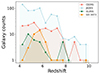 |
Fig. 1. Redshift distribution of the selected sample of spectroscopically confirmed galaxies at 4 ≤ z ≤ 10 in the different surveys considered in this work, as described in the main text. |
2.2. The JADES survey
We considered the third public data release of the survey (D’Eugenio et al. 2025) to select our sample. JADES provides both imaging and spectroscopy in the two GOODS fields. Spectroscopy consists of medium-depth and deep NIRSpec/MSA spectra of 4000 targets, covering the spectral range 0.6–5.3 μm and observed with both the low-dispersion prism (R = 30–300) and the three medium-resolution gratings (R = 500–1500). We refer to (D’Eugenio et al. 2025) for a complete description of observations, data reduction, sample selection, and target allocation. A total of 2053 redshifts were measured from multiple emission lines in this data release. The photometric catalog includes observation using the NIRCam wide-broad filters F090W, F115W, F150W, F200W, F277W, F356W, F444W, and the medium-broad filters F182M, F210M, F335M, F410M, F430M, F460M, F480M.
We selected galaxies with NIRSpec spectra at redshift 4 ≤ z ≤ 10. We selected galaxies with NIRCam photometry. Our sample thus includes 314 galaxies (240 with MR and 314 with prism) in the GOODS-South field and 255 galaxies (239 with MR and 246 with prism) in the GOODS-North field. The redshift distribution of the total sample of 569 galaxies is shown in lightblue in Fig. 1.
2.3. The GLASS survey
The GLASS survey obtained deep observations of galaxies in the Hubble Frontier Field cluster, Abell 2744, with both NIRCam photometry and NIRSpec spectroscopy. The public catalog includes galaxies observed with prism and the high-resolution (HR) G140H, G235H, and G395H grating. The public spectroscopic data release is found in Mascia et al. (2024b). We use the NIRSpec data reduced by the Cosmic Dawn Center, which is published on the DAWN JWST Archive (DJA)4. The photometric catalog includes observations using the NIRCam wide-broad filters F115W, F150W, F200W, F277W, F356W, F444W, and the medium-broad filters F410M (Merlin et al. 2024).
We selected galaxies with NIRSpec spectra at redshift 4 ≤ z ≤ 10 and with NIRCam photometry. Our sample includes 36 galaxies (23 with HR and 25 with prism) and its redshift distribution is shown in green in Fig. 1.
2.4. The GO-3073 program
The program observed the cluster Abell-2744 using the prism configuration of NIRSpec. In this study, we considered data obtained during the first epoch (October 24, 2023), divided into three visits, each with an exposure time of 6567 s. Unfortunately, an electrical short affected the third visit, so we excluded it from the final reduction. The data were processed using version 1.13.4 of the STScI Calibration Pipeline, with calibration reference data system (CRDS) mapping 1197. Further details on observations and data reduction are provided in Napolitano et al. (2025). The photometric catalog includes observations using the NIRCam wide-broad filters F090W, F115W, F150W, F200W, F277W, F356W, F444W (Merlin et al. 2024).
We selected 37 galaxies with 4 < z < 10 with NIRSpec, NIRCam photometry, and secure spectroscopic redshift. The redshift distribution of the sample is shown in orange in Fig. 1.
3. Data analysis
3.1. AGN removal and complete subsample
We first removed AGNs from our final sample based on the AGN sources identified in Roberts-Borsani et al. (2024) and Brooks et al. (2024). Their selection criteria for AGNs is based on broad + narrow component models to reproduce the Hα profiles, while the [OIII]λ5007 profile is reproduced by a single narrow component. Following this criterion, we removed 12 sources from the CEERS survey, 14 sources from the JADES survey, 1 source from the GLASS survey, and 2 sources from the GO-3073 program. Therefore, in the following sections, we consider a final sample of 761 galaxies. We note that our sample might still be contaminated by narrow obscured AGNs, but there is no clear method to select them at high z. We discuss this possible contamination in Appendix A.
We selected a subsample based on the detection limits of the surveys. We called this subsample the complete sample. We assumed a 5σ depth of 29.3 mag in F200W for a point source in the CEERS survey (Finkelstein et al. 2025), which is the shallowest survey we considered. The complete sample includes 570 galaxies above those depths.
3.2. Emission line measurements
To measure ξion in individual galaxies, we needed to estimate the luminosity of Balmer lines. In this case, we considered Hα and Hβ lines. For part of the analysis in the following sections, we also considered [OIII]λ5007 and the unresolved doublet [OII]λ3729 in the set of lines to measure.
For the CEERS survey, we considered the measurements included in the data release 0.9 (Arrabal Haro et al. in prep.). The set of measurements was performed using LiMe5 (Fernández et al. 2024), which is a library that provides a set of tools to fit the lines in astronomical spectra.
For consistency, we used the same code to measure the line for the sample in the other surveys. We considered one Gaussian to model the line profiles. For the galaxies in the GLASS survey and the GO-3073 program, we corrected the fluxes for magnification using the lens model presented in Bergamini et al. (2023). We also checked the flux calibration of the spectra based on the available photometry, and we corrected the observed fluxes by a factor of ∼30% of flux losses based on the median value in all the photometric bands. This correction does not depend sensibly on the wavelength, in agreement with what was found by Roberts-Borsani et al. (2024).
We corrected the line fluxes for dust reddening using the Calzetti et al. (2000) attenuation law. We considered the E(B − V) value derived from the SED fitting for galaxies, as described in the following Sect. 3.3. As a caveat, we did not consider the Balmer decrement in this project in order to have a homogeneous dust correction for all galaxies in the sample. When comparing E(B − V) values from Balmer lines and SED fitting, we find a difference by a factor of 0.47 (median) and 1.53 (mean). To avoid artificial trends induced by using different methods to estimate E(B − V) for the whole sample, we opted to consider the values from the SED fitting for dust attenuation. As we show in Sect. 3.5 and Appendix B, we find good agreement between the luminosities of Hα and Hβ, which corroborates the robustness of our dust correction.
3.3. SED fitting
We used BAGPIPES (Carnall et al. 2018) version 1.2.0 to estimate the physical parameters with the Bruzual & Charlot (2003) stellar population models. We fixed the redshift to the spectroscopic redshift. We considered a delayed exponential τ-model for the star formation history (SFH), where τ is the timescale of the decrease in the SFH. In the model, we consider an age ranging from 1 Myr to the age of the Universe at the observed redshift. We allowed the τ parameter to vary between 0.1 and 10 Gyr, and the metallicity to vary freely up to 0.5 Z⊙. The upper limit in stellar metallicity is based on the stellar mass-metallicity relation observed at z = 3.5 for a stellar mass of 1011 M⊙ (Llerena et al. 2022; Stanton et al. 2024). For the dust component, we considered the Calzetti et al. (2000) attenuation curve and let the AV parameter vary between 0 − 2 mag. We also included a nebular component in the model, and we let the ionization parameter freely vary between −4 and 0. We used the same recipe for all the galaxies in all surveys using the available photometry. The observed photometry of galaxies in the GLASS survey and in the GO-3073 program is corrected using the same lensing model available in Bergamini et al. (2023).
We also converted the dust-corrected L(Hα) to SFR assuming the calibration from Reddy et al. (2022) as SFR(Balmer) = L(Hα)×10−41.67. This is the most suited calibration according to the typical subsolar metallicities expected for our galaxies at z > 4, and reflects the greater efficiency of ionizing photon production in metal-poor stellar populations. The distribution of the sample along the main sequence at z = 6 (Iyer et al. 2018; Speagle et al. 2014) is displayed in Fig. 2. As a reference, we also show the main sequence from Calabrò et al. (2024b) that includes a wide range of redshifts between z = 4 and z = 10. Our sample is scattered around the main sequence, and the galaxies cover ∼3 dex in stellar mass and SFR. We note that there is no bias in stellar mass or SFR between the various subsamples depending on the considered survey. Nonetheless, less massive sources with M* ≲ 107.5 M⊙ tend to be above the main sequence, independently of the relation we use as reference.
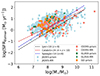 |
Fig. 2. Distribution of the full sample along the stellar mass-SFR plane. The dashed black and blue lines are the main-sequence of star-forming galaxies at z = 6 from Iyer et al. (2018) and Speagle et al. (2014), respectively. While the dashed red line represents the main-sequence at 4 < z < 10 from Calabrò et al. (2024b). The triangle symbols are upper limits based on Hα or on Hβ if an upper limit on Hα is not estimated. |
3.4. UV luminosity density
We determined the UV luminosity density by estimating the value of the rest-frame continuum at 1500 Å based on the SED model. For this purpose, we considered a synthetic top-hat filter of bandwidth 100 Å centered at 1500 Å to convolve with the SED model. Additionally, we followed Pahl et al. (2025) and estimated the uncertainty of the UV luminosity density by considering the mean uncertainty of the flux density in the observed filters covering the rest-frame from 1200 to 3000 Å. In this way, the error bars are motivated by nearby photometric constraints. We did not estimate the rest-frame continuum at 1500 Å from the spectra because of the lack of good S/N in the continuum in grating spectra. To obtain reliable and homogeneous estimates, we used the available photometry for all sources.
We corrected the obtained UV luminosity densities for dust reddening following the same procedure as for the emission line fluxes as described in Sect. 3.2. We lastly converted the dust-corrected UV luminosity densities to UV absolute magnitudes, which are analyzed in the following sections. In Fig. 3, we show the distribution of MUV versus redshift. Our sample covers a wide range of MUV (∼8 mag) with a mean value of MUV = −20.00 (σ = 1.61). In Appendix C we show the distribution of the measured Hα and Hβ emission line flux as a function of both redshift and MUV. We note that our complete sample includes galaxies with z ≲ 7 and MUV ≲ −18, which is the parameter space where our results are more robust.
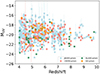 |
Fig. 3. Distribution of MUV as a function of redshift for the galaxies in the different surveys considered in our sample. |
3.5. Constraints on ξion
We estimated the ionizing photon production efficiency in a standard way, considering the model where ξion is given by
 (2)
(2)
where N(H0) is the ionizing photon rate in s−1 and LUV is the UV luminosity density at 1500 Å. In order to estimate the ionizing photon rate, we use the dust-corrected Hα luminosity when available as:
![Mathematical equation: $$ \begin{aligned} L(\mathrm{H}\alpha )[\mathrm{erg\,s}^{-1}] = 1.36\times 10^{-12} N(\mathrm{H}^0) [\mathrm{s}^{-1}], \end{aligned} $$](/articles/aa/full_html/2025/06/aa53251-24/aa53251-24-eq3.gif) (3)
(3)
which was derived from Leitherer & Heckman (1995) assuming no ionizing photons escape from the galaxy (fesc = 0) and case B recombination. For this conversion factor, it is assumed a Salpeter (1955) initial mass function (IMF) and a gas temperature of 10 000 K for the nebular emission in the evolutionary synthesis models. Alternatively, we use the dust-corrected Hβ luminosity as
![Mathematical equation: $$ \begin{aligned} L(\mathrm{H}\beta )[\mathrm{erg\,s}^{-1}] = 4.87\times 10^{-13} N(\mathrm{H}^0) [\mathrm{s}^{-1}]. \end{aligned} $$](/articles/aa/full_html/2025/06/aa53251-24/aa53251-24-eq4.gif) (4)
(4)
For galaxies with Hα and Hβ available, we checked that the values are in very good agreement (see Fig. B.1). We assume fesc = 0, meaning that all LyC photons are reprocessed into the Balmer lines. The derived ξion value can be considered as a lower limit since higher fesc will lead to a higher ξion. If Hα or Hβ are detected with S/N < 3, we put an upper 3σ limit in the ξion value for that galaxy. We considered an upper limit only if σ is lower than the detection limits of the surveys to avoid overestimating the upper limits. We also considered upper limits on Hα or upper limits on Hβ only when a limit on Hα is not possible to estimate. We obtained a mean value of log(ξion [Hz erg−1]) = 25.22 (σ = 0.42 dex) for the galaxies in the entire sample.
4. Results
4.1. Evolution of ξion with redshift
In Fig. 4 we show the evolution of ξion with redshift. The magenta squares are the median values in equally distributed redshift bins. For the median values, we considered the upper limits on ξion as half their values following the methodology in Calabrò et al. (2024b). In data science, imputation of upper limits with half the detection limit is a common approach, and simulation studies have found that this is a better choice compared to assuming the detection limit itself or a zero value, as it introduces the least bias into the estimates (Beal 2001). The error bars are the observed 1σ scatter within a given redshift bin. We note a shallow trend where the ξion increases with redshift from 4 ≤ z ≤ 10. Based on the median values, ξion increases from log(ξion [Hz erg−1]) = 25.09 at z ∼ 4.18 to log(ξion [Hz erg−1]) = 25.28 at z ∼ 7.14. The best linear fit of the median values considering the full sample leads to the relation log(ξion [Hz erg−1]) = (0.06 ± 0.012) × z+(24.82 ± 0.07). For galaxies at z ≳ 7.14, the median value of ξion is greater than the canonical value with a median value of log(ξion [Hz erg−1]) = 25.28.
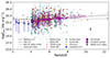 |
Fig. 4. Redshift evolution of ξion for the entire sample. The individual galaxies are in red, light-blue, green, and orange symbols, depending on the parent survey. The symbols with black edges are galaxies in the complete sample. The plus symbols are galaxies based on the grating (MR) configuration, while the square symbols are galaxies observed with the prism configuration. The triangle symbols are upper limits. The magenta symbols are the median values of ξion in equally populated bins of redshift. The magenta squares are the median values considering the full sample, while the magenta circles are the median values considering only the complete sample. The blue symbols are average values from Castellano et al. (2023). The red circles are individual galaxies or stacks from literature (Stark et al. 2015; Nakajima et al. 2016; Mármol-Queraltó et al. 2016; Bouwens et al. 2016; Matthee et al. 2017; Stark et al. 2017; Shivaei et al. 2018; Harikane et al. 2018; Vanzella et al. 2018; Faisst et al. 2019; Lam et al. 2019; De Barros et al. 2019; Emami et al. 2020; Nanayakkara et al. 2020; Castellano et al. 2022; Marques-Chaves et al. 2022; Stefanon et al. 2022; Prieto-Lyon et al. 2023; Bunker et al. 2023; Rinaldi et al. 2024; Roberts-Borsani et al. 2024; Mascia et al. 2024a; Saxena et al. 2024; Lin et al. 2024; Álvarez-Márquez et al. 2024; Hsiao et al. 2024; Calabrò et al. 2024a; Vanzella et al. 2024; Zavala et al. 2025). The dashed magenta line is the best fit of the median values of the full sample. The dashed line is the relation from Matthee et al. (2017), and the dotted-dashed line is the relation from Pahl et al. (2025). The canonical value of log ξion[Hz erg−1] ≈ 25.27, often assumed in reionization models, is highlighted in a horizontal dashed gray line for reference. The black symbol represents the median error of 0.07 dex in log ξion. |
Interestingly, our bins at z ∼ 4 − 5 are consistent within 1σ with the values found in Castellano et al. (2023), with the VANDELS galaxies at 2 ≤ z ≤ 5 using SED fitting to determine the ξion values. They found no significant evolution of ξion with redshift, but combining the two results, they suggest an increase in ξion from z ∼ 2 up to z ∼ 10. This trend also agrees with the relation found in Matthee et al. (2017) based on Hα emitters at z ∼ 2, which seems to be valid up to z ∼ 12, according to data from the literature, which are included in Fig. 4. We also compare our results with the recent work from Pahl et al. (2025) with a sample of CEERS and JADES galaxies from 1.06 < z < 6.71. We find that our results agree with the increase in ξion with redshift, but our median values are slightly lower than their observed trend, although consistent within the observed scatter.
We also find that the median values are below the usually assumed canonical value of ξion, for the bins at z < 7 and then become higher than this value at higher redshift. Given the large scatter, there are individual galaxies in each bin whose ξion values are above the canonical values. We do not find a significant difference in the observed trend if we include only galaxies in the complete sample. We still observe the increase in ξion with redshift up to z ∼ 6.92. We remark that the complete subsample extends up to z ∼ 7.5, which is the z completeness of our study. As we show in Appendix C, the completeness in MUV is up to magnitude ∼ − 18, which is similar to the completeness of other spectroscopic samples (e.g., Dottorini et al. 2025).
4.2. Relation between ξion and MUV
In Fig. 5 we show the relation between ξion and MUV. We find an increase in ξion with UV magnitude, which is also observed in individual galaxies. This is consistent with other works at 5 ≤ z ≤ 7, including galaxies in the emission-line galaxies and intergalactic gas in the EoR (EIGER; Kashino et al. 2023) survey, CEERS, JADES (Mascia et al. 2025), and also with works using photometry to estimate the ξion values at comparable redshifts (e.g., Simmonds et al. 2024) where we find a consistent slope. Our best fit of the median values is log(ξion [Hz erg−1]) = (0.15 ± 0.008) × MUV+(28.17 ± 0.17). According to this trend, fainter galaxies tend to show higher ξion values compared to brighter galaxies. In particular, galaxies in the fainter bins (median value ≳ − 19.36 mag) show > log(ξion [Hz erg−1]) = 25.28 higher than the canonical values. This trend is in the opposite direction compared with recent results from Pahl et al. (2025) and Begley et al. (2025), where they found that fainter galaxies are not the most efficient in producing ionizing photons but the brighter galaxies are. We also note that our relation perfectly agrees with that found in Simmonds et al. (2024) at z ∼ 5 − 6. If we consider only the galaxies in the complete sample, we find that the increasing trend is also found. Comparing with the literature, we find that our relation is in agreement with the ξion value found recently in a faint source in Vanzella et al. (2024) with MUV ∼ −12, which suggests faint sources are indeed efficient producers of ionizing photons.
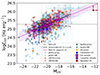 |
Fig. 5. Relation between ξion and MUV. The symbols are the same as in Fig. 4. The dotted-dashed line indicates the relation found in Pahl et al. (2025) for galaxies at 1.06 < z < 6.71. The solid black line indicates the relation found in Simmonds et al. (2024). The red circle indicates the faint source from Vanzella et al. (2024). |
In Fig. 6 we explore if the relation of ξion with MUV depends on the redshift. To this aim, we split the sample into three bins of redshifts: z = 4 − 5 (278 galaxies), z = 5 − 7 (366 galaxies), and z = 7 − 10 (117 galaxies). We find that for a given MUV, the galaxies with higher redshifts show higher ξion values, which is in agreement with the redshift evolution found in Sect. 4.1. The slopes of the relations do not vary sensibly at different redshifts (slopes between 0.15 and 0.21). In Table 1 we present the parameters of the best linear fits depending on the median redshift. We compare our results with the relations found in recent semi-analytic models with cold gas fractions and star-formation efficiencies obtained from hydrodynamical simulations (Mauerhofer et al. 2025). In particular, we compare our results with the models including an evolving IMF (eIMF) depending on redshift and metallicity, which becomes increasingly top-heavy with redshift or decreasing metallicity. Our results are consistent within 1σ with the increase in ξion with the increase in MUV found in the models at redshifts z ∼ 5 − 7 (Fig. 14 in Mauerhofer et al. 2025). At z ∼ 9 the same models suggest a flattening of the relation at ∼log(ξion [Hz erg−1]) = 25.5, which is consistent within 1σ with the values we obtained but not with the increasing trend we found in the bin with higher redshifts (median z = 7.45). The lower number of galaxies in this bin and the wider redshift range could explain the differences with the models. In any case, our results are consistent with the models with a top-heavy IMF.
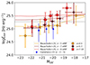 |
Fig. 6. Relation of ξion with MUV in bins of redshift. The red, dark red, and yellow symbols are the median values in the redshift bins. The dashed lines represent models with an eIMF at different redshifts from Mauerhofer et al. (2025). The dashed gray line indicates the canonical value for reference. |
Parameters of the best fits of the relation between ξion and MUV at different redshift, with log ξion = a × MUV+b
4.3. Total ionizing emissivity
We use the relations reported in Table 1 to estimate the total ionizing emissivity ṅion at the median redshifts in each bin. To do this calculation, we considered the UV luminosity functions of Bouwens et al. (2021) and a median fesc = 0.13 as recently inferred using indirect observational estimates at z ∼ 5 − 9 (Mascia et al. 2023, 2024a). This value does not depend substantially on MUV, at least in the magnitude range that can be currently explored. We also considered a maximum value of log(ξion [Hz erg−1]) = 26, which is in agreement with models of young metal-poor stellar populations (Raiter et al. 2010; Maseda et al. 2020) and simulations of PopIII populations (Lecroq et al. 2025). We integrated the luminosity function from MUV = −23 to different faint limits and present the result in Fig. 7 with limits MUV = −13 (plotted in red), MUV = −15 (in black), and MUV = −18 (in green). We performed 1000 Monte Carlo simulations assuming a normal distribution of the parameters of the UV luminosity functions and the best fits in Table 1, keeping the escape fraction constant. The plotted values are the corresponding median values, and the error bars are the 16th and 84th percentiles resulting from the simulations.
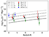 |
Fig. 7. Evolution of the total ionizing emissivity. The red, black, and green squares are our estimations after integrating from MUV = −23 to MUV = −13, MUV = −15, and MUV = −18, respectively. The black and green squares are shifted by 0.1 and 0.2 in redshift, respectively, for better visualization. The different lines represent IGM evolution models from Madau et al. (1999) for different ionized hydrogen clumping factors C. The blue squares are observational constraints obtained by observing the Lyα forest from Becker & Bolton (2013). |
We match observational constraints obtained by observing the Lyα forest from Becker & Bolton (2013). Our results are also consistent with IGM evolution models (Madau et al. 1999) and do not support recent claims for a budget-crisis and a too early end of reionization (e.g., Muñoz et al. 2024). We also find that the contribution of faint UV galaxies (−15 ≤ MUV ≤ −13) to the total ionizing emissivity becomes more important at higher redshift, increasing from ∼30% at z ∼ 4.4 to ∼47% at z ∼ 7.4 (Mascia et al. 2024a). On the other hand, the contribution of bright UV galaxies becomes less important at higher redshift, decreasing from ∼26% at z ∼ 4.4 to ∼9% at z ∼ 7.4. These results indicate that faint galaxies are the dominant sources of ionizing photons during the EoR.
4.4. Dependence of ξion on the physical properties
In this section we present our results on the relation between ξion and the physical properties obtained based on SED fitting. On the top panel in Fig. 8 we show the relation between ξion and the stellar mass. Based on the median values in stellar mass bins, we find a clear decrease in ξion with stellar mass. The best fit shown in Fig. 8 considers the median values. The best fit of the relation that we found is log(ξion [Hz erg−1]) = (−0.35 ± 0.01) × log(M⋆/M⊙)+(28.12 ± 0.11). This trend is in agreement with the one observed in VANDELS galaxies at lower redshifts (Castellano et al. 2023). We note a small offset, with the VANDELS sources showing slightly higher ξion values for a given stellar mass; however, this could be an effect of the method used to estimate ξion, since we are using Balmer lines. We note that in Castellano et al. (2023) SED modeling with BPASS was used (for more details, see in Sect. 4.5), and that their sample is complete for galaxies with stellar masses > 109.5 M⊙ which could lead to the offsets observed in the lower mass bins.
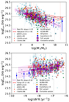 |
Fig. 8. Relation of ξion with physical properties of the galaxies. The top panel indicates the relation between ξion and stellar mass, while the bottom panel indicates the relation between ξion and the specific star-formation rate. The symbols are the same as in Fig. 4. In the top panel, the solid red line indicates the trend from the FLARES simulation at z = 6 (Seeyave et al. 2023), and the dashed red lines indicate their 3σ scatter. In the bottom panel, the solid red line represents the trend from the simulations in Yung et al. (2020b) at z = 6. The dashed red lines are the 16th and 84th percentiles. |
This decreasing trend is also observed in Simmonds et al. (2024) using NIRCam photometry for a sample of ∼670 galaxies at z ∼ 3.9 − 8.9. Interestingly, the two bins with lower stellar mass (median value ≲107.91 M⊙) show a median > log(ξion [Hz erg−1]) = 25.31 above the canonical value, which indicates that galaxies with lower stellar masses than this value tend to be efficient in producing ionizing photons. We also compare the trend we find with the results from simulations. In particular, we compare with the results from Seeyave et al. (2023) based on the FLARES simulation. They find a shallower decrease in ξion with redshift, with higher values of ξion for a given stellar mass. Our values are consistent with the 3σ scatter of their relation, in particular for low stellar masses. The differences could be attributed to using BPASS models in the simulations. According to Seeyave et al. (2023), the decreasing trend of ξion with stellar mass is due to the combined effects of increasing age and metallicity with increasing stellar mass, with metallicity likely playing a bigger role (compared to age) due to the weaker evolution of age with stellar mass.
On the bottom panel in Fig. 8 we show the relation between ξion and the sSFR. Based on the median values in sSFR bins, we find a clear increase in ξion with sSFR. The best fit of the relation that we found is log(ξion [Hz erg−1]) = (0.18 ± 0.04) × log(sSFR[yr−1])+(26.53 ± 0.30). This trend is also clear in individual galaxies. This trend is also in agreement with the one observed in VANDELS galaxies at lower redshifts (Castellano et al. 2023) in the common sSFR range covered by the two studies. Similar to the relation between ξion and stellar mass, we note that the bin with higher sSFR (median value ∼10−6.64 yr−1) shows a median log(ξion [Hz erg−1]) = 25.38, which is above the canonical value. This indicates that galaxies with sSFR higher than this value tend to be efficient producers of ionizing photons. Considering the complete sample, we note that galaxies with ∼10−6.59 yr−1) tend to show ξion above the canonical values as well, with a median value of log(ξion [Hz erg−1]) = 25.39. Comparing our results with the simulations from Yung et al. (2020b), we find a similar trend of increasing ξion with increasing sSFR, but with an offset. Despite this offset, the slope we find is similar to the one in the simulations.
In Fig. 9, we explore if the relations of ξion with stellar mass and sSFR depend on redshift. To this aim, we split the sample into the same three bins of redshifts as in Sect. 4.2. In Fig. 9, we show the median values of each bin. We find that for a given stellar mass, the galaxies with higher redshifts show higher ξion values, which is in agreement with the redshift evolution found in Sect. 4.1. Similar results are found with sSFR, with the galaxies in the bin z = 7 − 10 showing the highest ξion values. The slopes of the relations do not vary significantly at different redshifts (slopes between −0.33 and −0.44 for the relation between ξion and stellar mass, and slopes between 0.05 and 0.18 for the relation between ξion and sSFR), implying that the physical conditions leading to photon production in galaxies remain essentially the same across cosmic epochs i.e., for the same metallicity and ages, the efficiency is the same.
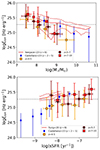 |
Fig. 9. Relation of ξion with physical properties of the galaxies in bins of redshift. The red, dark red, and yellow symbols are the median values in redshift bins. The dashed gray line is the canonical value for reference. |
4.5. Relation between ξion and EW([OIII])
The EW([OIII]) has been often used as a proxy for ξion. For example, Chevallard et al. (2018) found the relation marked with the solid line in Fig. 10 using a sample of 10 nearby analogs of primeval galaxies, which was then used in several works (Castellano et al. 2023). In Fig. 10, we show the relation between ξion and the EW([OIII]) for our sample. For the estimation of the EWs, we considered the continuum measured directly from the spectra based on Gaussian fitting. We find an increase in ξion with the EW([OIII]), where the more efficient ionizing photon producers are the galaxies that show the higher EW([OIII]). In particular, we show that the galaxies in the bins with higher EWs (median value ≳1800 Å) show values of > log(ξion [Hz erg−1]) = 25.40 above the canonical values. The best fit of the median values results in the relation log(ξion [Hz erg−1]) = (0.43 ± 0.02) × log(EW([OIII])[Å])+(23.99 ± 0.05). Compared to our trend, the Chevallard et al. (2018) relation is much steeper and tends to overpredict ξion values for the most extreme cases of EW([OIII]) and at the same time underpredict the ξion values in the cases with moderate EWs. A somewhat better agreement is found with the relation derived by Tang et al. (2019) for a sample of ∼200 intense [OIII] emitters at 1.3 < z < 2.4. We find good agreement in the bins with lower EWs, while in the more intense cases, our values tend to be lower than those predicted by these authors. Compared to the recent work by Pahl et al. (2025), we find slightly higher average values of ξion for a given EW. Nevertheless, the slope of the relation is consistent.
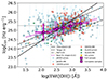 |
Fig. 10. Relation between ξion and EW([OIII]). The symbols are the same as in Fig. 4. The solid black line indicates the local relation from Chevallard et al. (2018). The dashed line indicates the relation from Tang et al. (2019) at 1.3 < z < 2.4. The dotted-dashed line indicates the relation found in Pahl et al. (2025) for galaxies at 1.06 < z < 6.71. |
We note that these offsets in the relations could also be the origin for the discrepancies observed in Fig. 8 when comparing our work to Castellano et al. (2023). Their ξion values are estimated using BEAGLE (Chevallard & Charlot 2016) and are consistent with the Chevallard et al. (2018) relation, which we found tends to overpredict the ξion for a given EW, in particular in galaxies with high EWs.
Recently, Laseter et al. (2024) found that modest [OIII] emitters (EW∼300–600 Å) may also show high values of ξion as we also show in individual galaxies in Fig. 10. One of the drivers of this effect could be the low metallicity in the systems where the EW([OIII]) is suppressed, but the fluxes of Balmer lines remain elevated. We analyze the relation of ξion with gas-phase metallicity in Sect. 4.6. This dependency on gas-phase metallicity would limit the use of [OIII] as a sole tracer of high z efficient ionizing systems.
4.6. Relation of ξion with O32 and gas-phase metallicity
In Fig. 11, we show the relation between ξion and O32=log([OIII]/[OII]). We also include the limit O32 > 0.69 from Flury et al. (2022) to separate strong LyC leakers found in the low redshift LyC survey galaxies. We find an increasing trend where the galaxies with higher O32 values show the highest ξion values. The best fit of the median values results in the relation log(ξion [Hz erg−1]) = (0.55 ± 0.07) × log([OIII]/[OII])+(24.77 ± 0.04). The bin with the higher O32 values (∼0.92) is above the threshold for strong LyC leakers, and it shows a median value log(ξion [Hz erg−1]) = 25.27, slightly above the canonical value. A similar trend was found in Shen et al. (2025) for galaxies at z ∼ 2 − 3. We find a similar slope of the relation compared to their median values, but our ξion values are slightly lower for a given O32 value. Since a high O32 ratio is one of the proposed proxies for a high escape of LyC radiation (Flury et al. 2022; Mascia et al. 2024a), our findings could imply that galaxies with high ionizing photon production efficiency are also those where the LyC escape is high. This has important implications for determining which sources contributed most to reionization. However, a high O32 is actually a necessary but not sufficient condition for a high escape fraction, and some authors actually find that at least for some classes of galaxies (e.g., Lyα emitters), production and escape of ionizing photons are anticorrelated (Saxena et al. 2024). We plan to investigate these links further in future works.
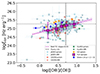 |
Fig. 11. Relation between ξion and O32. The symbols are the same as in Fig. 4. The blue squares indicate the median values from Shen et al. (2025) for galaxies at z ∼ 2 − 3. The vertical line indicates the demarcation line between strong and weak leakers from Flury et al. (2022). |
In Fig. 12, we show the relation between ξion and gas-phase metallicity. We estimate the metallicity from the R23 = ([OIII]λλ4959,5007+[OII]λλ3727,3729)/Hβ calibration presented in Sanders et al. (2024) for galaxies at z = 2.1 − 8.7. Given that this relation is bivaluated, we also used the O32 calibration in Sanders et al. (2024). We consider as metallicity estimation the metallicity from the R23 calibration that is closer to the value from the O32 calibration. We find a shallow decreasing trend with metallicity, with the metal-poor galaxies showing the higher ξion values. The best fit of the median values results in the relation log(ξion [Hz erg−1]) = (−0.18 ± 0.08) × (log(O/H)+12)+(26.64 ± 0.69). According to the best fit of the median values, galaxies with metallicities ≲10% solar tend to show ξion values above the canonical value and are efficient in producing LyC photons. We note that this relation is consistent with a flat slope at 3σ, and a larger sample would be needed to better constrain the dependency of ξion on metallicity.
5. Summary and conclusions
We selected a sample of 761 galaxies at z = 4 − 10 with NIRSpec spectra in four JWST surveys (CEERS, JADES, GLASS, and GO-3073) in this large study of ξion conducted via spectroscopy. We estimated their physical properties using available JWST and HST photometry for performing SED fitting using BAGPIPES (Carnall et al. 2018), assuming a delayed exponential model for the SFH. We constrained the ξion values based on Balmer lines (Hα or Hβ) and estimated the gas-phase metallicity using R23 and O32 calibrations for high z sources. We investigated the evolution of ξion with redshift and its relation to the physical properties of the galaxies. Our main results are the following:
-
We find an evolution of the ionizing photon production efficiency of star-forming galaxies with higher values of ξion at higher redshifts. The evolution is mild, with the best linear relation given by log(ξion [Hz erg−1]) = (0.06 ± 0.012) × z+(24.82 ± 0.07). This trend is consistent with other results at lower redshifts. According to this relation, a median value of log(ξion [Hz erg−1]) = 25.12 is inferred at z = 4.5, while a median value of log(ξion [Hz erg−1]) = 25.32 is inferred at z = 7.5.
-
We find an increase in ξion with increasing MUV. The best fit results in the relation log(ξion [Hz erg−1]) = (0.15 ± 0.008) × MUV+(28.17 ± 0.17). We also evaluated the ξion versus MUV relation in separate redshift bins and found that the slopes of the different relations stay constant, although with increasing offset. The relations are consistent with the predictions of recent models, with the eIMF becoming top-heavy at higher redshifts and lower metallicity.
-
Assuming our values of ξion as a function of MUV and redshift, and a mean escape fraction of 0.13 as recently derived by Mascia et al. (2025), we calculated the evolution of the total ionizing emissivity. Our results show that galaxies can sustain reionization, provided that the clumpiness factor does not exceed 10 and is consistent with low redshift constraints by the Lyα forest. We also find that faint UV galaxies (−15 ≤ MUV ≤ −13) are the main contributors of ionizing photons in the early stages of reionization.
-
We find a decrease in ξion values with increasing M⋆ with the best fit resulting in the relation log(ξion [Hz erg−1]) = (−0.35 ± 0.01) × log(M⋆/M⊙)+(28.12 ± 0.11). We find an increase in ξion with increasing sSFR, similar to other studies at lower redshifts. The best fit results in the relation log(ξion [Hz erg−1]) = (0.18 ± 0.04) × log(sSFR[yr−1])+(26.53 ± 0.30). This indicates that low-mass, faint in the UV, and with high levels of sSFRs galaxies tend to be efficient in producing ionizing photons. The slopes of the above relations do not significantly change with redshift, implying that the conditions for photon production do not change and that the redshift evolution is only due to the different statistical properties of populations at each redshift.
-
We find an increase in ξion with EW(O[III]). The best fit results in the relation log(ξion [Hz erg−1]) = (0.43 ± 0.02) × log(EW([OIII])[Å])+(23.99 ± 0.05). Compared to our trend, the widely used relation found by Chevallard et al. (2018) is much steeper and tends to overpredict the ξion values in the most extreme cases of EW([OIII]) and, to the contrary, underpredict the ξion values in the cases with moderate EWs. We instead find better agreement with the relation proposed by Tang et al. (2019), at least in the bins with lower EWs, while in the bins with higher EWs, our ξion values are lower.
-
We find an increase in ξion with O32 ratio. The best fit results in the relation log(ξion [Hz erg−1]) = (0.55 ± 0.07) × log([OIII]/[OII])+(24.77 ± 0.04). Since O32 is one of the most used proxies for a high escape fraction of LyC photons, this could imply that leakers are also efficient in producing ionizing photons, in contrast to some previous findings.
-
Finally, we find a decrease in ξion with gas-phase metallicity. The best fit results in the relation log(ξion [Hz erg−1]) = (−0.18 ± 0.08) × (log(O/H)+12)+(26.64 ± 0.69). The rather shallow relation indicates that metallicity does not play such a key role in determining the photon production efficiency.
Overall, we find that faint low-mass galaxies with high levels of sSFRs present the best conditions for an efficient production of ionizing photons, while low metallicity seems to play a more marginal role in setting such conditions, given the shallow trend observed. We also find indications that galaxies with high photon production efficiency may also be those in which the conditions for high leakage of such photons are present, since they share properties similar to low redshift LyC leakers – namely, high O32, faint UV magnitudes, and low-stellar masses. Such galaxies could therefore be primarily responsible for cosmic reionization: we plan to further investigate the link between ionizing photon production and escape in a follow-up study. In general, although we do find that high redshift galaxies have higher ξion compared to the low redshift sources with similar properties, our median values for the galaxy population during the EoR are not as extreme as those found by other authors (e.g., Maseda et al. 2020; Prieto-Lyon et al. 2023; Atek et al. 2024; Saxena et al. 2024). In agreement with other authors (e.g., Simmonds et al. 2024), our results, therefore, do not support recent claims of a budget crisis, i.e. that the total ionizing photons generated by galaxies are much higher than previously thought. Such a scenario, together with significant escape fractions, could provide enough photons to end reionization too early, which would be in contrast to Lyman α forest results (Muñoz et al. 2024).
Acknowledgments
We thank the anonymous referee for the detailed review and useful suggestions that helped to improve this paper. We wish to thank all our colleagues in the CEERS collaboration for their hard work and valuable contributions to this project. We thank Pietro Bergamini for providing us with the magnification factors for the lensed sources. MLl acknowledges support from the INAF Large Grant 2022 “Extragalactic Surveys with JWST” (PI L. Pentericci), the PRIN 2022 MUR project 2022CB3PJ3 – First Light And Galaxy aSsembly (FLAGS) funded by the European Union – Next Generation EU, and INAF Mini-grant “Galaxies in the epoch of Reionization and their analogs at lower redshift” (PI M. Llerena). RA acknowledges support of grant PID2023-147386NB-I00 funded by MICIU/AEI/10.13039/501100011033 and by ERDF/EU, and the Severo Ochoa grant CEX2021-001131-S This work is based on observations made with the NASA/ESA/CSA James Webb Space Telescope (JWST). The JWST data presented in this article were obtained from the Mikulski Archive for Space Telescopes (MAST) at the Space Telescope Science Institute. The specific observations analyzed are associated with program JWST-GO-3073 and can be accessed via DOI. We acknowledge support from INAF Mini-grant “Reionization and Fundamental Cosmology with High-Redshift Galaxies”. This work has made extensive use of Python packages astropy (Astropy Collaboration 2018), numpy (Harris et al. 2020), Matplotlib (Hunter 2007) and LiMe (Fernández et al. 2024).
References
- Álvarez-Márquez, J., Colina, L., Crespo Gómez, A., et al. 2024, A&A, 686, A85 [NASA ADS] [CrossRef] [EDP Sciences] [Google Scholar]
- Arrabal Haro, P., Dickinson, M., Finkelstein, S. L., et al. 2023, ApJ, 951, L22 [NASA ADS] [CrossRef] [Google Scholar]
- Asplund, M., Grevesse, N., Sauval, A. J., & Scott, P. 2009, ARA&A, 47, 481 [NASA ADS] [CrossRef] [Google Scholar]
- Astropy Collaboration (Price-Whelan, A. M., et al.) 2018, AJ, 156, 123 [Google Scholar]
- Atek, H., Labbé, I., Furtak, L. J., et al. 2024, Nature, 626, 975 [NASA ADS] [CrossRef] [Google Scholar]
- Backhaus, B. E., Trump, J. R., Cleri, N. J., et al. 2022, ApJ, 926, 161 [NASA ADS] [CrossRef] [Google Scholar]
- Bagley, M. B., Finkelstein, S. L., Koekemoer, A. M., et al. 2023, ApJ, 946, L12 [NASA ADS] [CrossRef] [Google Scholar]
- Beal, S. L. 2001, J. Pharmacokinetics Pharmacodynamicsp, 28, 504 [Google Scholar]
- Becker, G. D., & Bolton, J. S. 2013, MNRAS, 436, 1023 [Google Scholar]
- Begley, R., McLure, R. J., Cullen, F., et al. 2025, MNRAS, 537, 3245 [NASA ADS] [CrossRef] [Google Scholar]
- Beichman, C. A., Rieke, M., Eisenstein, D., et al. 2012, in Space Telescopes and Instrumentation 2012: Optical, Infrared, and Millimeter Wave, eds. M. C. Clampin, G. G. Fazio, H. A. MacEwen, & J. M. Oschmann, SPIE Conf. Ser., 8442, 84422N [NASA ADS] [CrossRef] [Google Scholar]
- Bergamini, P., Acebron, A., Grillo, C., et al. 2023, ApJ, 952, 84 [NASA ADS] [CrossRef] [Google Scholar]
- Bertin, E., & Arnouts, S. 1996, A&AS, 117, 393 [NASA ADS] [CrossRef] [EDP Sciences] [Google Scholar]
- Bosman, S. E. I., Davies, F. B., Becker, G. D., et al. 2022, MNRAS, 514, 55 [NASA ADS] [CrossRef] [Google Scholar]
- Bouwens, R. J., Smit, R., Labbé, I., et al. 2016, ApJ, 831, 176 [Google Scholar]
- Bouwens, R. J., Oesch, P. A., Stefanon, M., et al. 2021, AJ, 162, 47 [NASA ADS] [CrossRef] [Google Scholar]
- Brooks, M., Simons, R. C., Trump, J. R., et al. 2024, arXiv e-prints [arXiv:2410.07340] [Google Scholar]
- Bruzual, G., & Charlot, S. 2003, MNRAS, 344, 1000 [NASA ADS] [CrossRef] [Google Scholar]
- Bunker, A. J., Saxena, A., Cameron, A. J., et al. 2023, A&A, 677, A88 [NASA ADS] [CrossRef] [EDP Sciences] [Google Scholar]
- Bushouse, H., Eisenhamer, J., Dencheva, N., et al. 2022, https://doi.org/10.5281/zenodo.7041998 [Google Scholar]
- Calabrò, A., Castellano, M., Zavala, J. A., et al. 2024a, ApJ, 975, 245 [CrossRef] [Google Scholar]
- Calabrò, A., Pentericci, L., Santini, P., et al. 2024b, A&A, 690, A290 [NASA ADS] [CrossRef] [EDP Sciences] [Google Scholar]
- Calzetti, D., Armus, L., Bohlin, R. C., et al. 2000, ApJ, 533, 682 [NASA ADS] [CrossRef] [Google Scholar]
- Carnall, A. C., McLure, R. J., Dunlop, J. S., & Davé, R. 2018, MNRAS, 480, 4379 [Google Scholar]
- Castellano, M., Pentericci, L., Cupani, G., et al. 2022, A&A, 662, A115 [NASA ADS] [CrossRef] [EDP Sciences] [Google Scholar]
- Castellano, M., Belfiori, D., Pentericci, L., et al. 2023, A&A, 675, A121 [NASA ADS] [CrossRef] [EDP Sciences] [Google Scholar]
- Chevallard, J., & Charlot, S. 2016, MNRAS, 462, 1415 [NASA ADS] [CrossRef] [Google Scholar]
- Chevallard, J., Charlot, S., Senchyna, P., et al. 2018, MNRAS, 479, 3264 [Google Scholar]
- Coil, A. L., Aird, J., Reddy, N., et al. 2015, ApJ, 801, 35 [Google Scholar]
- De Barros, S., Oesch, P. A., Labbé, I., et al. 2019, MNRAS, 489, 2355 [NASA ADS] [CrossRef] [Google Scholar]
- D’Eugenio, F., Cameron, A. J., Scholtz, J., et al. 2025, ApJS, 277, 4 [Google Scholar]
- Dottorini, D., Calabrò, A., Pentericci, L., et al. 2025, A&A, 698, A234 [NASA ADS] [CrossRef] [EDP Sciences] [Google Scholar]
- Eisenstein, D. J., Johnson, B. D., Robertson, B., et al. 2023, ApJS, submitted, [arXiv:2310.12340] [Google Scholar]
- Emami, N., Siana, B., Alavi, A., et al. 2020, ApJ, 895, 116 [NASA ADS] [CrossRef] [Google Scholar]
- Faisst, A. L., Capak, P. L., Emami, N., Tacchella, S., & Larson, K. L. 2019, ApJ, 884, 133 [NASA ADS] [CrossRef] [Google Scholar]
- Fan, X., Strauss, M. A., Becker, R. H., et al. 2006, AJ, 132, 117 [NASA ADS] [CrossRef] [Google Scholar]
- Fernández, V., Amorín, R., Firpo, V., & Morisset, C. 2024, A&A, 688, A69 [NASA ADS] [CrossRef] [EDP Sciences] [Google Scholar]
- Finkelstein, S. L., D’Aloisio, A., Paardekooper, J.-P., et al. 2019, ApJ, 879, 36 [Google Scholar]
- Finkelstein, S. L., Bagley, M. B., Ferguson, H. C., et al. 2023, ApJ, 946, L13 [NASA ADS] [CrossRef] [Google Scholar]
- Finkelstein, S. L., Bagley, M. B., Arrabal Haro, P., et al. 2025, ApJ, 983, L4 [Google Scholar]
- Flury, S. R., Jaskot, A. E., Ferguson, H. C., et al. 2022, ApJ, 930, 126 [NASA ADS] [CrossRef] [Google Scholar]
- Gardner, J. P., Mather, J. C., Clampin, M., et al. 2006, Space Sci. Rev., 123, 485 [Google Scholar]
- Gardner, J. P., Mather, J. C., Abbott, R., et al. 2023, PASP, 135, 068001 [NASA ADS] [CrossRef] [Google Scholar]
- Grogin, N. A., Kocevski, D. D., Faber, S. M., et al. 2011, ApJS, 197, 35 [NASA ADS] [CrossRef] [Google Scholar]
- Harikane, Y., Ouchi, M., Shibuya, T., et al. 2018, ApJ, 859, 84 [NASA ADS] [CrossRef] [Google Scholar]
- Harris, C. R., Millman, K. J., van der Walt, S. J., et al. 2020, Nature, 585, 357 [NASA ADS] [CrossRef] [Google Scholar]
- Hsiao, T. Y.-Y., Abdurro’uf, Coe, D., et al. 2024, ApJ, 973, 8 [NASA ADS] [CrossRef] [Google Scholar]
- Hunter, J. D. 2007, Comput. Sci. Eng., 9, 90 [NASA ADS] [CrossRef] [Google Scholar]
- Iyer, K., Gawiser, E., Davé, R., et al. 2018, ApJ, 866, 120 [Google Scholar]
- Jakobsen, P., Ferruit, P., Alves de Oliveira, C., et al. 2022, A&A, 661, A80 [NASA ADS] [CrossRef] [EDP Sciences] [Google Scholar]
- Juneau, S., Bournaud, F., Charlot, S., et al. 2014, ApJ, 788, 88 [NASA ADS] [CrossRef] [Google Scholar]
- Kashino, D., Lilly, S. J., Matthee, J., et al. 2023, ApJ, 950, 66 [CrossRef] [Google Scholar]
- Koekemoer, A. M., Faber, S. M., Ferguson, H. C., et al. 2011, ApJS, 197, 36 [NASA ADS] [CrossRef] [Google Scholar]
- Lam, D., Bouwens, R. J., Labbé, I., et al. 2019, A&A, 627, A164 [NASA ADS] [CrossRef] [EDP Sciences] [Google Scholar]
- Laseter, I. H., Maseda, M. V., Simmonds, C., et al. 2024, arXiv e-prints [arXiv:2412.04542] [Google Scholar]
- Lecroq, M., Charlot, S., Bressan, A., et al. 2025, A&A, 695, A17 [NASA ADS] [CrossRef] [EDP Sciences] [Google Scholar]
- Leitherer, C., & Heckman, T. M. 1995, ApJS, 96, 9 [NASA ADS] [CrossRef] [Google Scholar]
- Lin, Y.-H., Scarlata, C., Williams, H., et al. 2024, MNRAS, 527, 4173 [Google Scholar]
- Llerena, M., Amorín, R., Cullen, F., et al. 2022, A&A, 659, A16 [NASA ADS] [CrossRef] [EDP Sciences] [Google Scholar]
- Madau, P., Haardt, F., & Rees, M. J. 1999, ApJ, 514, 648 [CrossRef] [Google Scholar]
- Madau, P., Giallongo, E., Grazian, A., & Haardt, F. 2024, ApJ, 971, 75 [NASA ADS] [CrossRef] [Google Scholar]
- Maiolino, R., Scholtz, J., Curtis-Lake, E., et al. 2024, A&A, 691, A145 [NASA ADS] [CrossRef] [EDP Sciences] [Google Scholar]
- Mármol-Queraltó, E., McLure, R. J., Cullen, F., et al. 2016, MNRAS, 460, 3587 [Google Scholar]
- Marques-Chaves, R., Schaerer, D., Álvarez-Márquez, J., et al. 2022, MNRAS, 517, 2972 [CrossRef] [Google Scholar]
- Mascia, S., Pentericci, L., Calabrò, A., et al. 2023, A&A, 672, A155 [NASA ADS] [CrossRef] [EDP Sciences] [Google Scholar]
- Mascia, S., Pentericci, L., Calabrò, A., et al. 2024a, A&A, 685, A3 [NASA ADS] [CrossRef] [EDP Sciences] [Google Scholar]
- Mascia, S., Roberts-Borsani, G., Treu, T., et al. 2024b, A&A, 690, A2 [NASA ADS] [CrossRef] [EDP Sciences] [Google Scholar]
- Mascia, S., Pentericci, L., Llerena, M., et al. 2025, A&A, submitted, [arXiv:2501.08268] [Google Scholar]
- Maseda, M. V., Bacon, R., Lam, D., et al. 2020, MNRAS, 493, 5120 [Google Scholar]
- Matthee, J., Sobral, D., Best, P., et al. 2017, MNRAS, 465, 3637 [NASA ADS] [CrossRef] [Google Scholar]
- Mauerhofer, V., Dayal, P., Haehnelt, M. G., et al. 2025, A&A, 696, A157 [NASA ADS] [CrossRef] [EDP Sciences] [Google Scholar]
- Merlin, E., Santini, P., Paris, D., et al. 2024, A&A, 691, A240 [NASA ADS] [CrossRef] [EDP Sciences] [Google Scholar]
- Muñoz, J. B., Mirocha, J., Chisholm, J., Furlanetto, S. R., & Mason, C. 2024, MNRAS, 535, L37 [CrossRef] [Google Scholar]
- Naidu, R. P., Tacchella, S., Mason, C. A., et al. 2020, ApJ, 892, 109 [NASA ADS] [CrossRef] [Google Scholar]
- Nakajima, K., Ellis, R. S., Iwata, I., et al. 2016, ApJ, 831, L9 [Google Scholar]
- Nanayakkara, T., Brinchmann, J., Glazebrook, K., et al. 2020, ApJ, 889, 180 [Google Scholar]
- Napolitano, L., Castellano, M., Pentericci, L., et al. 2025, A&A, 693, A50 [NASA ADS] [CrossRef] [EDP Sciences] [Google Scholar]
- Oke, J. B., & Gunn, J. E. 1983, ApJ, 266, 713 [NASA ADS] [CrossRef] [Google Scholar]
- Pahl, A., Topping, M. W., Shapley, A., et al. 2025, ApJ, 981, 134 [Google Scholar]
- Prieto-Lyon, G., Strait, V., Mason, C. A., et al. 2023, A&A, 672, A186 [NASA ADS] [CrossRef] [EDP Sciences] [Google Scholar]
- Raiter, A., Schaerer, D., & Fosbury, R. A. E. 2010, A&A, 523, A64 [NASA ADS] [CrossRef] [EDP Sciences] [Google Scholar]
- Reddy, N. A., Topping, M. W., Shapley, A. E., et al. 2022, ApJ, 926, 31 [NASA ADS] [CrossRef] [Google Scholar]
- Rinaldi, P., Caputi, K. I., Iani, E., et al. 2024, ApJ, 969, 12 [NASA ADS] [CrossRef] [Google Scholar]
- Roberts-Borsani, G., Treu, T., Shapley, A., et al. 2024, ApJ, 976, 193 [NASA ADS] [CrossRef] [Google Scholar]
- Robertson, B. E. 2022, ARA&A, 60, 121 [NASA ADS] [CrossRef] [Google Scholar]
- Robertson, B. E., Furlanetto, S. R., Schneider, E., et al. 2013, ApJ, 768, 71 [Google Scholar]
- Rosdahl, J., Katz, H., Blaizot, J., et al. 2018, MNRAS, 479, 994 [NASA ADS] [Google Scholar]
- Salpeter, E. E. 1955, ApJ, 121, 161 [Google Scholar]
- Sanders, R. L., Shapley, A. E., Topping, M. W., Reddy, N. A., & Brammer, G. B. 2024, ApJ, 962, 24 [NASA ADS] [CrossRef] [Google Scholar]
- Saxena, A., Bunker, A. J., Jones, G. C., et al. 2024, A&A, 684, A84 [NASA ADS] [CrossRef] [EDP Sciences] [Google Scholar]
- Seeyave, L. T. C., Wilkins, S. M., Kuusisto, J. K., et al. 2023, MNRAS, 525, 2422 [NASA ADS] [CrossRef] [Google Scholar]
- Shen, L., Papovich, C., Matharu, J., et al. 2025, ApJ, 980, L45 [Google Scholar]
- Shivaei, I., Reddy, N. A., Siana, B., et al. 2018, ApJ, 855, 42 [Google Scholar]
- Simmonds, C., Tacchella, S., Hainline, K., et al. 2024, MNRAS, 527, 6139 [Google Scholar]
- Speagle, J. S., Steinhardt, C. L., Capak, P. L., & Silverman, J. D. 2014, ApJS, 214, 15 [Google Scholar]
- Stanton, T. M., Cullen, F., McLure, R. J., et al. 2024, MNRAS, 532, 3102 [Google Scholar]
- Stark, D. P., Walth, G., Charlot, S., et al. 2015, MNRAS, 454, 1393 [Google Scholar]
- Stark, D. P., Ellis, R. S., Charlot, S., et al. 2017, MNRAS, 464, 469 [NASA ADS] [CrossRef] [Google Scholar]
- Stefanon, M., Bouwens, R. J., Illingworth, G. D., et al. 2022, ApJ, 935, 94 [NASA ADS] [CrossRef] [Google Scholar]
- Tang, M., Stark, D. P., Chevallard, J., & Charlot, S. 2019, MNRAS, 489, 2572 [NASA ADS] [CrossRef] [Google Scholar]
- Tang, M., Stark, D. P., Chen, Z., et al. 2023, MNRAS, 526, 1657 [NASA ADS] [CrossRef] [Google Scholar]
- Treu, T., Roberts-Borsani, G., Bradac, M., et al. 2022, ApJ, 935, 110 [NASA ADS] [CrossRef] [Google Scholar]
- Vanzella, E., Nonino, M., Cupani, G., et al. 2018, MNRAS, 476, L15 [Google Scholar]
- Vanzella, E., Loiacono, F., Messa, M., et al. 2024, A&A, 691, A251 [NASA ADS] [CrossRef] [EDP Sciences] [Google Scholar]
- Wright, G. S., Wright, D., Goodson, G. B., et al. 2015, PASP, 127, 595 [NASA ADS] [CrossRef] [Google Scholar]
- Yang, J., Wang, F., Fan, X., et al. 2020, ApJ, 904, 26 [Google Scholar]
- Yung, L. Y. A., Somerville, R. S., Finkelstein, S. L., et al. 2020a, MNRAS, 496, 4574 [NASA ADS] [CrossRef] [Google Scholar]
- Yung, L. Y. A., Somerville, R. S., Popping, G., & Finkelstein, S. L. 2020b, MNRAS, 494, 1002 [NASA ADS] [CrossRef] [Google Scholar]
- Zavala, J. A., Castellano, M., Akins, H. B., et al. 2025, Nat. Astron., 9, 155 [Google Scholar]
Appendix A: Possible obscured AGNs
In Sect. 3.1 we removed unobscured AGNs with broad Balmer lines from our sample galaxies at z = 4 − 10. However, we note that our sample can still exhibit a contribution from obscured, narrow AGNs. To analyze this possible contamination, in this section we investigate the location of galaxies in some emission-line diagnostics. In particular, we analyze the OHNO diagram proposed in Backhaus et al. (2022) to separate the galaxies ionized by massive stars from those galaxies ionized by AGNs. We analyze the subsample of galaxies with detected [NeIII]λ3870 and the blended [OII]λλ3726,3728 line. In Fig. A.1 we show the location of this subsample in the OHNO diagram. We note that all these galaxies are above the demarcation line and, therefore, could be AGNs. However, we remark that star-forming galaxies are also found in this locus, as seen in Fig. 6 in Backhaus et al. (2022). Therefore, it is not clear that this subsample is AGN-based only on this diagnostic diagram. For this reason, we analyze an alternative diagram that can be applied to this subsample. We choose the Mass-Excitation (MEx; Juneau et al. 2014) diagram, shown in Fig. A.2. Based on this diagnostic diagram, we note that most of the galaxies in our sample are star-forming galaxies. The subsample of AGN candidates based on the OHNO diagram is also in the locus of star-forming galaxies in the MEx diagram. Only a few candidates lie above the demarcation line from Juneau et al. (2014), but not above the one from Coil et al. (2015), at z ∼ 2.3. We note, however, that the MeX diagram is not calibrated at the redshifts considered in this paper (Coil et al. 2015).
As a conclusion, based on these two diagnostics that are applicable to the galaxies in our sample, we cannot define a clear subsample of narrow AGNs. For this reason, we keep these sources in the final sample analyzed in this paper.
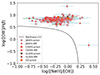 |
Fig. A.1. OHNO diagram for the galaxies in our sample. The symbols are the same as in Fig. 4. The dashed line indicates the demarcation line from Backhaus et al. (2022) to separate star-forming galaxies from AGNs. The AGN region lies above this line based on this diagnostic. Based on this diagnostic diagram, AGN candidates are shown as symbols with red edges. |
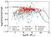 |
Fig. A.2. MEx diagram for the galaxies in our sample. The symbols are the same as in Fig. 4. The AGN candidates from Fig. A.1 are shown as symbols with red edges. The dashed black line indicates the demarcation between star-forming galaxies and AGNs, according to Juneau et al. (2014). The dashed-dotted black line is the demarcation at z ∼ 2 (Coil et al. 2015). |
We explore whether there are biases in the relation we found in 4 due to the inclusion of these AGN candidates in our sample. In Fig. A.3, we show the location of the AGN candidates based on the OHNO diagram, in the relation between ξion and redshift, indicated in Fig. 4. They show a wide range of redshifts from z ∼ 4 − 8 and a wide range of ξion values. They follow the trend of the median values of the full sample, which suggests there is no bias due to these candidates in the overall trend. Similar results are found if we analyze the relation of ξion with the stellar mass, as shown in Fig. A.4. We show they have a wide range of stellar masses ≳107.5 M⊙ and ξion values. Similarly, they follow the trend that is observed with the median values of the full sample. Lastly, in Fig. A.5 we check the location of the AGN candidates in the relation of ξion with MUV. Similarly, we find that they show a wide range of MUV and ξion values. They are in general bright (MUV≲-19) compared to the full sample, which suggests this may be the reason [NeIII]λ3870 is detected in these candidates, rather than being ionized by AGNs. We also find that these candidates follow the trend observed with the median values of the full sample. Overall, we find that including these not secure AGN candidates in our sample does not affect the trends we find in this paper.
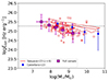 |
Fig. A.4. AGN candidates in the relation between ξion and stellar mass. The symbols are the same as in Fig. 8. The red symbols represent the AGN candidates from Fig. A.1. |
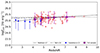 |
Fig. A.3. AGN candidates in the evolution of ξion with redshift. The symbols are the same as in Fig. 4. The red symbols represent the AGN candidates from Fig. A.1. |
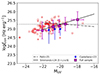 |
Fig. A.5. AGN candidates in the relation between ξion and MUV. The symbols are the same as in Fig. 5. The red symbols are the AGN candidates from Fig. A.1. |
Appendix B: ξion from Balmer lines
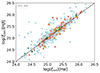 |
Fig. B.1. Comparison between ξion determined from Hα and Hβ luminosities. The symbols represent individual galaxies in the sample with simultaneous detection of Hα and Hβ. The symbols are the same as in Fig. 4. |
In Fig. B.1 we show a comparison between the values of ξion determined from Hα and Hβ for the subsample of galaxies in the full sample with simultaneous detections of both Balmer lines. We find that there is good agreement between the two estimations with a median difference of 0.05 dex. Due to this fact, we do not introduce a bias when mixing both estimations in the galaxies where Hα is undetected.
Appendix C: Observed Balmer fluxes
In Fig. C.1 we show the relation between the observed fluxes of Balmer lines as a function of redshift and MUV. We note that both Hα and Hβ cover a wide range of fluxes (∼2dex). For Hα this distribution is uniform across all the redshifts (z ≲ 7) while for Hβ we measured fluxes < 2 × 10⁻¹⁸ erg s−1 cm−2 for galaxies at z ≳ 7 and some of them are upper limits in flux. We also note that most of the complete subsample includes galaxies up to z ∼ 7 for the two lines.
Regarding the relation between ξion and MUV, we find a decreasing trend in the fluxes with increasing MUV, which indicates that the faintest UV galaxies show also fainter Balmer lines compared to brighter UV galaxies. This is in agreement with the distribution along the MS shown in Fig. 2. In our sample we do not include UV bright passive galaxies as seen in Fig. C.1. We also note that most of the galaxies in the complete subsample show MUV ≲ −18. We need to take into account these ranges in redshift and MUV when analyzing the results since in these ranges we have a complete sample and the results are more robust.
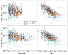 |
Fig. C.1. Observed fluxes of Hα (top panels) and Hβ (bottom panels) as a function of redshift (left panels) and MUV (right panels). The symbols are the same as in Fig. 4. |
All Tables
Parameters of the best fits of the relation between ξion and MUV at different redshift, with log ξion = a × MUV+b
All Figures
|
Fig. 1. Redshift distribution of the selected sample of spectroscopically confirmed galaxies at 4 ≤ z ≤ 10 in the different surveys considered in this work, as described in the main text. |
| In the text | |
|
Fig. 2. Distribution of the full sample along the stellar mass-SFR plane. The dashed black and blue lines are the main-sequence of star-forming galaxies at z = 6 from Iyer et al. (2018) and Speagle et al. (2014), respectively. While the dashed red line represents the main-sequence at 4 < z < 10 from Calabrò et al. (2024b). The triangle symbols are upper limits based on Hα or on Hβ if an upper limit on Hα is not estimated. |
| In the text | |
|
Fig. 3. Distribution of MUV as a function of redshift for the galaxies in the different surveys considered in our sample. |
| In the text | |
|
Fig. 4. Redshift evolution of ξion for the entire sample. The individual galaxies are in red, light-blue, green, and orange symbols, depending on the parent survey. The symbols with black edges are galaxies in the complete sample. The plus symbols are galaxies based on the grating (MR) configuration, while the square symbols are galaxies observed with the prism configuration. The triangle symbols are upper limits. The magenta symbols are the median values of ξion in equally populated bins of redshift. The magenta squares are the median values considering the full sample, while the magenta circles are the median values considering only the complete sample. The blue symbols are average values from Castellano et al. (2023). The red circles are individual galaxies or stacks from literature (Stark et al. 2015; Nakajima et al. 2016; Mármol-Queraltó et al. 2016; Bouwens et al. 2016; Matthee et al. 2017; Stark et al. 2017; Shivaei et al. 2018; Harikane et al. 2018; Vanzella et al. 2018; Faisst et al. 2019; Lam et al. 2019; De Barros et al. 2019; Emami et al. 2020; Nanayakkara et al. 2020; Castellano et al. 2022; Marques-Chaves et al. 2022; Stefanon et al. 2022; Prieto-Lyon et al. 2023; Bunker et al. 2023; Rinaldi et al. 2024; Roberts-Borsani et al. 2024; Mascia et al. 2024a; Saxena et al. 2024; Lin et al. 2024; Álvarez-Márquez et al. 2024; Hsiao et al. 2024; Calabrò et al. 2024a; Vanzella et al. 2024; Zavala et al. 2025). The dashed magenta line is the best fit of the median values of the full sample. The dashed line is the relation from Matthee et al. (2017), and the dotted-dashed line is the relation from Pahl et al. (2025). The canonical value of log ξion[Hz erg−1] ≈ 25.27, often assumed in reionization models, is highlighted in a horizontal dashed gray line for reference. The black symbol represents the median error of 0.07 dex in log ξion. |
| In the text | |
|
Fig. 5. Relation between ξion and MUV. The symbols are the same as in Fig. 4. The dotted-dashed line indicates the relation found in Pahl et al. (2025) for galaxies at 1.06 < z < 6.71. The solid black line indicates the relation found in Simmonds et al. (2024). The red circle indicates the faint source from Vanzella et al. (2024). |
| In the text | |
|
Fig. 6. Relation of ξion with MUV in bins of redshift. The red, dark red, and yellow symbols are the median values in the redshift bins. The dashed lines represent models with an eIMF at different redshifts from Mauerhofer et al. (2025). The dashed gray line indicates the canonical value for reference. |
| In the text | |
|
Fig. 7. Evolution of the total ionizing emissivity. The red, black, and green squares are our estimations after integrating from MUV = −23 to MUV = −13, MUV = −15, and MUV = −18, respectively. The black and green squares are shifted by 0.1 and 0.2 in redshift, respectively, for better visualization. The different lines represent IGM evolution models from Madau et al. (1999) for different ionized hydrogen clumping factors C. The blue squares are observational constraints obtained by observing the Lyα forest from Becker & Bolton (2013). |
| In the text | |
|
Fig. 8. Relation of ξion with physical properties of the galaxies. The top panel indicates the relation between ξion and stellar mass, while the bottom panel indicates the relation between ξion and the specific star-formation rate. The symbols are the same as in Fig. 4. In the top panel, the solid red line indicates the trend from the FLARES simulation at z = 6 (Seeyave et al. 2023), and the dashed red lines indicate their 3σ scatter. In the bottom panel, the solid red line represents the trend from the simulations in Yung et al. (2020b) at z = 6. The dashed red lines are the 16th and 84th percentiles. |
| In the text | |
|
Fig. 9. Relation of ξion with physical properties of the galaxies in bins of redshift. The red, dark red, and yellow symbols are the median values in redshift bins. The dashed gray line is the canonical value for reference. |
| In the text | |
|
Fig. 10. Relation between ξion and EW([OIII]). The symbols are the same as in Fig. 4. The solid black line indicates the local relation from Chevallard et al. (2018). The dashed line indicates the relation from Tang et al. (2019) at 1.3 < z < 2.4. The dotted-dashed line indicates the relation found in Pahl et al. (2025) for galaxies at 1.06 < z < 6.71. |
| In the text | |
|
Fig. 11. Relation between ξion and O32. The symbols are the same as in Fig. 4. The blue squares indicate the median values from Shen et al. (2025) for galaxies at z ∼ 2 − 3. The vertical line indicates the demarcation line between strong and weak leakers from Flury et al. (2022). |
| In the text | |
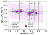 |
Fig. 12. Relation between ξion and gas-phase metallicity. The symbols are the same as in Fig. 4. |
| In the text | |
|
Fig. A.1. OHNO diagram for the galaxies in our sample. The symbols are the same as in Fig. 4. The dashed line indicates the demarcation line from Backhaus et al. (2022) to separate star-forming galaxies from AGNs. The AGN region lies above this line based on this diagnostic. Based on this diagnostic diagram, AGN candidates are shown as symbols with red edges. |
| In the text | |
|
Fig. A.2. MEx diagram for the galaxies in our sample. The symbols are the same as in Fig. 4. The AGN candidates from Fig. A.1 are shown as symbols with red edges. The dashed black line indicates the demarcation between star-forming galaxies and AGNs, according to Juneau et al. (2014). The dashed-dotted black line is the demarcation at z ∼ 2 (Coil et al. 2015). |
| In the text | |
|
Fig. A.4. AGN candidates in the relation between ξion and stellar mass. The symbols are the same as in Fig. 8. The red symbols represent the AGN candidates from Fig. A.1. |
| In the text | |
|
Fig. A.3. AGN candidates in the evolution of ξion with redshift. The symbols are the same as in Fig. 4. The red symbols represent the AGN candidates from Fig. A.1. |
| In the text | |
|
Fig. A.5. AGN candidates in the relation between ξion and MUV. The symbols are the same as in Fig. 5. The red symbols are the AGN candidates from Fig. A.1. |
| In the text | |
|
Fig. B.1. Comparison between ξion determined from Hα and Hβ luminosities. The symbols represent individual galaxies in the sample with simultaneous detection of Hα and Hβ. The symbols are the same as in Fig. 4. |
| In the text | |
|
Fig. C.1. Observed fluxes of Hα (top panels) and Hβ (bottom panels) as a function of redshift (left panels) and MUV (right panels). The symbols are the same as in Fig. 4. |
| In the text | |
Current usage metrics show cumulative count of Article Views (full-text article views including HTML views, PDF and ePub downloads, according to the available data) and Abstracts Views on Vision4Press platform.
Data correspond to usage on the plateform after 2015. The current usage metrics is available 48-96 hours after online publication and is updated daily on week days.
Initial download of the metrics may take a while.