| Issue |
A&A
Volume 675, July 2023
|
|
|---|---|---|
| Article Number | A121 | |
| Number of page(s) | 11 | |
| Section | Extragalactic astronomy | |
| DOI | https://doi.org/10.1051/0004-6361/202346069 | |
| Published online | 07 July 2023 | |
The ionizing photon production efficiency of bright z ∼ 2 − 5 galaxies
1
INAF – OAR, Via Frascati 33, 00078 Monte Porzio Catone, Roma, Italy
e-mail: This email address is being protected from spambots. You need JavaScript enabled to view it.
2
Sorbonne Université, CNRS, UMR 7095, Institut d’Astrophysique de Paris, 98 bis bd Arago, 75014 Paris, France
3
Department of Physics, University of Oxford, Denys Wilkinson Building, Keble Road, Oxford OX1 3RH, UK
4
Centre for Astrophysics Research, Department of Physics, Astronomy and Mathematics, University of Hertfordshire, Hatfield AL10 9AB, UK
5
University of Bologna – Department of Physics and Astronomy “Augusto Righi” (DIFA), Via Gobetti 93/2, 40129 Bologna, Italy
6
INAF – OAS, Osservatorio di Astrofisica e Scienza dello Spazio di Bologna, Via Gobetti 93/3, 40129 Bologna, Italy
7
Cosmic Dawn Center (DAWN), Niels Bohr Institute, University of Copenhagen, Jagtvej 128, 2200 Copenhagen, Denmark
8
Niels Bohr Institute, University of Copenhagen, Blegdamsvej 17, 2100 Copenhagen, Denmark
9
INAF – Istituto di Astrofisica Spaziale e Fisica Cosmica, Via A. Corti 12, 20133 Milan, Italy
10
Instituto de Astrofisica, Facultad de Ciencias Exactas, Universidad Andres Bello, Fernandez Concha 700, Las Condes, Santiago RM, Chile
11
Institute for Astronomy, University of Edinburgh, Royal Observatory, Edinburgh EH9 3HJ, UK
12
European Southern Observatory, Alonso de Córdova 3107, Vitacura, Santiago de Chile, Chile
13
Department of Astronomy, University of Geneva, 51 Chemin Pegasi, 1290 Versoix, Switzerland
14
Sub-department of Astrophysics, University of Oxford, Keble Road, Oxford OX1 3RH, UK
15
Department of Physics and Astronomy, University College London, Gower Street, London WC1E 6BT, UK
16
IBEX Innovations, Sedgefield, Stockton-on-Tees TS21 3FF, UK
17
Department of Physics & Astronomy, University of California, Los Angeles, 430 Portola Plaza, Los Angeles, CA 90095, USA
Received:
2
February
2023
Accepted:
22
May
2023
Abstract
Aims. We investigate the production efficiency of ionizing photons (ξion∗) of 1174 galaxies with secure redshift at z = 2 − 5 from the VANDELS survey to determine the relation between ionizing emission and physical properties of bright and massive sources.
Methods. We constrained ξion∗ and galaxy physical parameters by means of spectrophotometric fits performed with the BEAGLE code. The analysis exploits the multi-band photometry in the VANDELS fields and the measurement of UV rest-frame emission lines (CIII]λ1909, HeIIλ1640, and OIII]λ1666) from deep VIMOS spectra.
Results. We find no clear evolution of ξion∗ with redshift within the probed range. The ionizing efficiency slightly increases at fainter MUV and bluer UV slopes, but these trends are less evident when the analysis is restricted to a complete subsample at log(Mstar/M⊙) > 9.5. We find a significant trend of increasing ξion∗ with increasing EW(Lyα), with an average log(ξion∗/Hz erg−1) > 25 at EW > 50 Å and a higher ionizing efficiency for high-EW CIII]λ1909 and OIII]λ1666 emitters. The most significant correlations are found with respect to stellar mass, specific star formation rate (sSFR), and SFR surface density (ΣSFR). The relation between ξion∗ and sSFR increases monotonically from log(ξion∗/Hz erg−1)∼24.5 at log(sSFR) ∼ −9.5 yr−1 to ∼25.5 at log(sSFR) ∼ −7.5 yr−1. This relation has a low scatter and only a weak dependence on mass. The objects above the main sequence of star formation consistently have higher than average ξion∗. A clear increase in ξion∗ with ΣSFR is also found, with log(ξion∗/Hz erg−1) > 25 for objects at ΣSFR > 10 M⊙ yr−1 kpc−2.
Conclusions. Bright (MUV ≲ 20) and massive (log(Mstar/M⊙)≳9.5) galaxies at z = 2 − 5 have a moderate ionizing efficiency. However, the correlation between ξion∗ and sSFR, together with the known increase in the average sSFR with redshift at fixed stellar mass, suggests that similar galaxies in the epoch of reionization can be efficient sources of ionizing photons. The availability of sSFR and ΣSFR as proxies for ξion∗ can be fundamentally important in determining the role of galaxy populations at z ≳ 10 that were recently discovered by the James Webb Space Telescope in the onset of reionization.
Key words: galaxies: high-redshift / galaxies: evolution / dark ages, reionization, first stars
© ESO 2023
 Open Access article, published by EDP Sciences, under the terms of the Creative Commons Attribution License (http://creativecommons.org/licenses/by/4.0), which permits unrestricted use, distribution, and reproduction in any medium, provided the original work is properly cited.
1. Introduction
Investigating the ionizing emission of star-forming galaxies is key to understanding how galaxies form stars and affect the surrounding environment. In particular, this investigation is fundamental to constrain the role played by high-redshift galaxies in the epoch of reionization (EoR) of the inter-galactic medium at z ≳ 6 (IGM; Dayal & Ferrara 2018; Robertson 2022). The rate of ionizing photons escaping into the IGM from a galaxy population is  , where ρUV is the UV luminosity density,
  is the ionizing photon production efficiency per unit UV luminosity, and fesc is the fraction of ionizing photons that is leaked into the galaxy surroundings. The ρUV can be constrained by measuring the galaxy UV luminosity function (e.g., Castellano et al. 2010; Bouwens et al. 2021). The escape fraction of ionizing photons can only be directly constrained at z ≲ 3 − 4 (e.g., Vanzella et al. 2016; Marchi et al. 2017; Steidel et al. 2018; Pahl et al. 2021), but the recent findings on indirect estimators of fesc in low-redshift galaxies (e.g., Izotov et al. 2018a,b; Flury et al. 2022) enable the first constraints on the escape fraction of galaxies in the EoR (e.g., Lin et al. 2023; Mascia et al. 2023a). To constrain the contribution of high-redshift galaxies to the EoR, much effort has also been spent to study the ionizing photon production efficiency
  as a function of redshift and of galaxy properties.
Theoretical models predict a mild evolution of  with redshift. Typical values in the reionization epoch are thought to lie in the range log(
 /Hz erg−1)≃25.1 − 25.5. The ionizing photon production efficiency is predicted to be a factor of about 2 higher in low-mass galaxies due to their lower metallicity, which likely drives trends of increasing
  with decreasing SFR, UV slope and UV luminosity, and increasing sSFR (Wilkins et al. 2016; Ceverino et al. 2019; Yung et al. 2020). However, model predictions have been found to critically depend on the adopted stellar population synthesis (SPS) models: The inclusion of binary stellar populations increases
  by a factor of ≳2 in simulated galaxies (e.g., Ma et al. 2016; Yung et al. 2020).
Direct observational constraints on the ionizing efficiency  can be obtained from the spectroscopic measurement of the Balmer emission lines after correcting for dust attenuation (e.g., Schaerer et al. 2016; Shivaei et al. 2018). Similarly, photometric measurements of the flux from optical emission lines can be used when spectroscopic observations are not available (e.g., Bouwens et al. 2016). As an alternative, it has been shown that
  can be estimated from the equivalent width (EW) of the [OIII]λ4959, 5007 doublet (Chevallard et al. 2018; Reddy et al. 2018; Tang et al. 2019), rest-frame UV colors (Duncan & Conselice 2015), or UV rest-frame emission lines (Stark et al. 2015a). The reference ionizing efficiency assumed in reionization scenarios is log(
 /Hz erg−1)≃25.2 − 25.3 (Robertson et al. 2013), which is consistent with the value measured in Lyman-break galaxy (LBG) samples at z ∼ 4 − 5 and with predictions from theoretical models (Wilkins et al. 2016).
However, measurements show a wide range of values for different classes of objects, ranging from the ∼24.8 of local compact star-forming galaxies (CSFGs; Izotov et al. 2017) and z ∼ 2 H-α emitters (Matthee et al. 2017) to extreme log( /Hz erg−1)≃26.3 of faint Lyman-α emitters at z ∼ 4 − 5. Higher than average ionizing efficiencies log(
 /Hz erg−1)≳25.5 have also been found in local Lyman-continuum leakers (Schaerer et al. 2016), Lyman-α emitters at z ∼ 3 − 5 (Harikane et al. 2018; Sobral & Matthee 2019), and strong-line emitters at z > 2 (Nakajima et al. 2016; Tang et al. 2019). It has been shown that
  remains approximately constant as a function of the observed UV luminosity at fixed redshift, while it increases in objects with blue UV slopes (Bouwens et al. 2016; Shivaei et al. 2018; Lam et al. 2019; Izotov et al. 2021). A correlation between
  and the specific star formation rate (sSFR) has been found by Izotov et al. (2021) on CSFGs at z ≤ 1 and is apparent at higher redshifts from the correlation between
  and EW(Hα) found by Faisst et al. (2019; 3.9 < z < 4.9), Emami et al. (2020; 1.4 < z < 2.7), and Prieto-Lyon et al. (2023; 3 < z < 7).
Only a few constraints are available for galaxies in the EoR. Some objects at z ≳ 7 have been found to have very high ionizing efficiencies (≳25.7; e.g., Stark et al. 2015b, 2017; Endsley et al. 2021a, 2023; Stefanon et al. 2022; Fujimoto et al. 2023). In other cases, the  has been estimated to be consistent with or slightly higher than the canonical range assumed for high-redshift galaxies (Castellano et al. 2022b; Schaerer et al. 2022). The suggested trend of an increasing typical
  with redshift likely arises from a change in the underlying mixture of galaxy populations that is eventually driven by an evolution in physical parameters. Similarly, the discrepancies among the
  estimates can result from the different sampling of the various galaxy populations by the different selection techniques.
  has been found to increase in objects with a high ionization state, young ages, and low metallicity, and it is also affected by star formation burstiness, the initial mass function (IMF), and the evolution of stellar populations (Shivaei et al. 2018; Chisholm et al. 2019). It is thus fundamental to investigate the relation between galaxy properties and ionizing efficiency in order to fully constrain the role of star-forming galaxies in the EoR.
We exploit a large sample of galaxies at z ∼ 2 − 5 from the VANDELS survey (McLure et al. 2018; Pentericci et al. 2018) that provides robust measurements of their spectroscopic redshift, spectral energy distribution (SED), and UV emission lines to investigate the relation between  and the physical parameters of the galaxies. The paper is organized as follows: The sample is presented in Sect. 2, and in Sect. 3, we discuss the spectrophotometric fit we used to constrain
  and other physical properties. The analysis of the variation in
  with the observed properties and physical parameters is presented in Sect. 4. The results are summarized in Sect. 5. Throughout the paper, we adopt AB magnitudes (Oke & Gunn 1983), a Chabrier (2003) IMF, and a Λ-CDM concordance model (H0 = 70 km s−1 Mpc−1, ΩM = 0.3, and ΩΛ = 0.7).
2. VANDELS sample
We used data from VANDELS, a recently completed ESO public spectroscopic survey carried out using the VIMOS spectrograph on the Very Large Telescope (VLT). VANDELS targets were selected in the UKIDSS Ultra Deep Survey (UDS) and the Chandra Deep Field South (CDFS). VANDELS footprints are centered on the HST areas observed by the CANDELS program (Grogin et al. 2011; Koekemoer et al. 2011), but because of the VIMOS field of view, the observed areas are twice as large: For the outer areas that are not covered by the HST imaging data, new photometric catalogs were assembled.
The survey description and initial target selection strategies are described in McLure et al. (2018), and data reduction and redshift determination can be found in Pentericci et al. (2018). The fourth and final data release that we used is fully described in Garilli et al. (2021) and contains the redshifts of ∼2100 sources and the photometric catalogs described above1. In particular, the redshifts were derived using the code pandora.ez (Garilli et al. 2010), which cross-correlates the spectra with a series of galaxy templates. The redshifts were then checked visually by four different members of the collaboration. The reliability of the redshifts was quantified with a quality flag (QF) in the following way: 0 means no redshift could be determined; 1 indicates a 50% probability that the redshift is correct; 2 indicates a 70–80% probability that the redshift is correct; 3 and 4 indicate a 95% and 100% probability that the redshift is correct, respectively; and finally, 9 means that the spectrum shows a single emission line and that the redshift corresponds to the most probable identification. We analyzed all sources with 2 ≤ z ≤ 5 and a secure redshift here, that is, QF = 3 and = 4.
We excluded 13 AGN selected as in Bongiorno et al. (in prep.). The objects are considered to be likely AGN because they either had an X-ray counterpart from Luo et al. (2017) or Kocevski et al. (2018; for the CDFS and UDS fields respectively) within a radius of 1.5″, showed typical broad emission lines, or showed high-ionization narrow emission lines with line ratios typical of AGN (according to the diagnostics described in Feltre et al. 2016). The final sample comprises 1174 galaxies, 604 of which are in CDFS and 577 are in the UDS field. All objects were selected as star-forming galaxies or LBGs in the VANDELS target preparation, except for 3 sources that were initially classified as potential AGN on the basis of their SED, and one Herschel-detected source. We verified that their inclusion does not affect the analysis presented here.
2.1. Photometric measurements
For the objects in our sample, we used the VANDELS photometric catalogs described by McLure et al. (2018) for the outer CDFS and UDS areas, the CANDELS photometric catalog by Galametz et al. (2013) for the UDS-HST field, and the improved CANDELS catalog including both photometry from Guo et al. (2013) and the Ks-band HAWKI data from Fontana et al. (2014) for the CDFS-HST field. The objects in our sample are provided with a measurement of their UV slope performed by fitting the available broadband photometric measurements sampling the 1230–2750 Å rest-frame range as described in Calabrò et al. (2021). We find that the UV slope is robustly measured when at least three photometric bands are used in the fit and when the uncertainty on the measurement is σ(β) < 0.5. This condition is met for 810 objects out of the 1174 in the parent sample. For each of these objects, the UV slope determination was also used to estimate the rest-frame UV magnitude, MUV, from a simple interpolation of the continuum at 1600 Å. Finally, we used the equivalent radii measured by Calabrò et al. (2022) for 749 objects covered by F814W HST imaging. This subsample has a median F814W magnitude of 25.2, corresponding to a signal-to-noise ratio (S/N) ∼ 20, enabling an accurate measurement of their size (see also Ribeiro et al. 2016, for the relevant method).
2.2. Spectroscopic measurements
The measurements we used come from the official VANDELS spectroscopic catalog (Talia et al., in prep.). Specifically, we used a Gaussian fit obtained by slinefit (Schreiber et al. 2018) for the Lyα line and direct integration measurements for the other UV emission lines. We visually inspected the spectra in the Lyα range and assigned a flag to indicate whether a single Gaussian provided a good fit to the line. We here only use EW(Lyα) for the 565 objects in our sample with a robust Gaussian fit of the line.
The direct integration measurements were performed using PyLick, a tool developed to measure Lick-like indices and continuum breaks. It was extensively tested on galaxies from the LEGA-C survey (van der Wel et al. 2016) and on VANDELS sources (Borghi et al. 2022). The parameters that are to be defined are the integration windows and the bandpasses for the blue and red part of the continuum. For the absorption lines, the bandpasses were already defined in the literature (Maraston et al. 2009; Leitherer et al. 2011), but for the emission lines, they are not standard and were newly defined on the basis of a high S/N (∼35 pixel−1) composite spectrum of all sources with VANDELS quality flag 3 and 4 (see Talia et al. for more details).
We here use measurements of HeIIλ1640, OIII]λ1666, and CIII]λ1909. We did not consider CIVλ1548 because it is a blend of stellar and nebular emission, with a profile resulting from the mixture of emission and absorption features. The properties of VANDELS CIV-emitters, including their ionizing efficiency, are discussed in a companion paper (Mascia et al. 2023b). For the UV lines of interest, the following windows were used: 1634 − 1654 Å for the HeIIλ1640 emission (blue and red continuum windows at 1614 − 1632 and 1680 − 1705 Å, respectively), 1663 − 1668 Å for OIII]λ1666 (continuum: 1614 − 1632 and 1680 − 1705Å), and 1897 − 1919 Å for CIII]λ1909 (continuum: 1815 − 1839 and 1932 − 1948 Å, respectively). The uncertainties on the measurements are evaluated by PyLick following the S/N method by Cardiel et al. (1998). Talia et al. found that the error spectra produced by the data reduction pipeline underestimate the noise level by a factor of about 2 on average with respect to the noise r.m.s. measured on the object spectra. Therefore, they applied an a posteriori correction factor to the error spectra that were used to derive measurement uncertainties.
3. Spectrophotometric fitting with BEAGLE
We measured the physical parameters of the VANDELS galaxies, including the ionizing budget, by means of a spectrophotometric fit performed with the tool BEAGLE (Chevallard & Charlot 2016) using the most recent version of the Bruzual & Charlot (2003) stellar population synthesis models (see Vidal-García et al. 2017, for details). Nebular emission was modeled self-consistently as described in Gutkin et al. (2016) by processing stellar emission with the photoionization code CLOUDY (Ferland et al. 2013). The fit was performed by fitting the integrated lines plus continuum fluxes measured as described in Sect. 2. The redshift was fixed at the spectroscopic value, which is the one provided with the VANDELS final release, with the exception of the objects with a CIII]λ1909 detection at an S/N > 3, for which we used the relevant systemic redshift determination (Calabrò et al. 2022).
3.1. BEAGLE configuration
The BEAGLE SED-fitting runs were performed with a configuration similar to the one adopted to estimate the ionizing efficiency of very high-redshift galaxies (Stark et al. 2017; Castellano et al. 2022b). The templates are based on a Chabrier (2003) initial mass function, and their metallicity lies in the range −2.2 ≤ log(Z/Z⊙)≤0.25. The configuration adopted the most flexible parametric star formation history (SFH) allowed by the code, which is an exponentially delayed function (SFR(t)∝t ⋅ exp(−t/τ)) plus an ongoing constant burst. This SFH model allows analyzing objects with both rising and declining star formation histories (Carnall et al. 2019) and accurate estimates of the global properties of both main-sequence and starburst galaxies (Ciesla et al. 2017).
The duration of the final constant SFR phase is a free parameter in BEAGLE that we chose to fix to 10 Myr, considering that most of the nebular emission is generated by reprocessed light of massive stars with ages of 3–10 Myr (Kennicutt 1998; Kennicutt & Evans 2012). We adopted uniform priors on the SFH exponential timescale (7.0 ≤ τ/log(yr) ≤ 10.5), stellar mass (7.0 ≤ log(M/M⊙) ≤ 12), star formation rate (0.0 ≤ log(SFR/M⊙ yr−1) ≤ 3.0), and maximum stellar age (7.0 ≤ log(Age/yr) ≤ age of the Universe). Attenuation by dust was treated following the Charlot & Fall (2000) model combined with the Chevallard et al. (2013) prescriptions for geometry and inclination effects, assuming an effective V-band optical depth in the range −3.0 ≤ log(τV)≤0.7, with a fixed fraction μ = 0.4 arising from dust in the diffuse ISM. The interstellar metallicity ZISM was assumed to be identical to the stellar metallicity, and the dust-to-metal mass ratio and ionization parameter were left free in the ranges 0.1 ≤ ξd ≤ 0.5 and −4.0 ≤ log(Us)≤ − 1.0, respectively. In the following analysis, we use the best-fit parameters obtained by BEAGLE from the maximum of the posterior probability distribution functions. The 68% confidence level uncertainty on each parameter was measured from the relevant marginal probability distribution. For the derived parameter  , which was not expressly sampled over in the fitting, we provide the mean and 68% confidence level interval of the relevant weighted distribution derived from the MULTINEST samples (Eq. (9) in Feroz & Hobson 2008; see also Chevallard & Charlot 2016).
We show the main properties of the sample in Fig. 1. The VANDELS objects are mostly bright (MUV < −20) massive galaxies whose redshift distribution peaks at z ∼ 3 − 4, with tails covering the entire z ∼ 2 − 5 range. The stellar mass distribution covers the range log(Mstar/M⊙) = 8 − 11, but it is clearly incomplete at low masses. We compared the mass distribution of the VANDELS sample to that of all objects with photometric redshift 2 < z < 5 in the official CANDELS catalogs (Santini et al. 2015). They are perfectly consistent at log(Mstar/M⊙) > 9.5 when the CANDELS counts are scaled by a factor of four to take the target sampling of the spectroscopic survey into account. Instead, the VANDELS target selection criteria clearly yield an incompleteness at lower masses. For this reason, we discuss the entire sample and the mass-complete subsample at log(Mstar/M⊙) > 9.5 separately below.
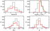 |
Fig. 1. Main properties of the VANDELS sample (black) and of the objects with log(Mstar/M⊙) > 9.5 (red). The spectroscopic redshifts are from VANDELS DR4, stellar masses (Mstar) have been estimated with BEAGLE as discussed in Sect. 3, and the UV magnitudes (MUV) and slopes (β) have been measured from the observed photometry (Sect. 2.1). The green continuous line in the top right panel shows the Mstar distribution for all CANDELS objects at z = 2 − 5 in UDS and GOODS-South from Santini et al. (2015), scaled by a factor of 4 to take the target sampling of the spectroscopic survey into account. |
3.2. Accuracy of the spectrophotometric analysis
Our approach exploits a combined spectrophotometric fit to estimate  and other physical parameters of the galaxies at the same time. As a test of the reliability of the fit, including spectroscopic lines, we compared the measured line fluxes to the relevant best-fit fluxes from BEAGLE. As shown in Fig. 2, BEAGLE can accurately reproduce the three observed lines across the entire flux range we probed.
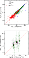 |
Fig. 2. Tests of the accuracy of the BEAGLE SED-fitting results. Top: comparison between the BEAGLE best-fit flux and the observed flux of the lines used in the spectrophotometric fitting. Bottom: comparison between the |


We then assessed the dependence of our results on the adopted BEAGLE configuration through the analysis of a representative subsample of 200 objects at z = 3 − 4. In order to test the effect of different attenuation laws, we performed the fit adopting the Calzetti et al. (2000) law or the SMC extinction law by Pei (1992). We find that the  values from our reference run that assumed a Charlot & Fall (2000) attenuation are consistent (Δ log(
 ) < 0.01) with those found with a Calzetti et al. (2000) law, but they are slightly lower on average (Δ log(
 ) = 0.065) than those based on the SMC extinction.
We then tested the dependence of the  estimates on the assumed SFH. We find a that the spectrophotometric fit returns slightly higher
  values (∼0.1 dex; see also Mascia et al. 2023b) when 5 Myr is assumed instead of a 10 Myr timescale as the duration of the ongoing star formation episode. We then performed a fit using only the photometric information and setting the duration of the ongoing star formation episode to 100 Myr, which matches the SFR timescale probed by UV-integrated light. We found an almost fixed log(
 /Hz erg−1)∼25.2 for all sources, while the SFR and Mstar values are consistent with the values in the reference spectrophotometric fit, but with a fraction of objects with an SFR lower by a factor 1.5 and correspondingly higher stellar mass. Instead, a fit using photometry alone and a 10 Myr duration of the ongoing star formation episode provided
  values that were statistically consistent with those obtained for the same SFH and including spectroscopic information, with the exception of a fraction of objects with EW(OIII]λ1666) > 3 for which the ionizing efficiency was found to be lower. This result indicates that the inclusion of spectroscopic measurements enables more accurate constraints, although the estimated efficiencies are largely affected by photometric information in objects with a low EW of the UV lines.
In order to perform a direct test of the robustness of our  measurement, we exploited observation from the NIRVANDELS survey that targeted the VANDELS fields with MOSFIRE to measure optical rest-frame emission lines. A detailed description of the NIRVANDELS observations can be found in Cullen et al. (2021). We found that 30 objects at z ∼ 3.15 − 3.78 in our sample have a clear [OIII]λ4959, 5007 detection in their MOSFIRE K-band spectra, enabling an estimate of
  from EW(OIII) using Eq. (3.1) in Chevallard et al. (2018). In addition, 9 objects at z ∼ 2.23–2.49 have detection of both Hα and Hβ, enabling a measurement of
  using standard conversions from the dust-corrected Hα luminosity (e.g., Shivaei et al. 2018). We measured the total flux of the Balmer lines and of the [OIII] λλ4959,5007 doublet with a Gaussian fit of each line component. For the z > 3 subsample, we used the measured broadband photometry at the corresponding observed wavelength to determine the EW([OIII]) because the continuum is undetected in the spectra. For the objects with a detection of the Balmer lines, we first corrected the measured Hα luminosity for dust extinction on the basis of the Balmer decrement assuming a Calzetti et al. (2000) attenuation law and an intrinsic ratio (Hα/Hβ) = 2.86 (see, e.g., Domínguez et al. 2013). We then applied the relation in Leitherer & Heckman (1995) to convert L(Hα) into an intrinsic Lyman-continuum photon production rate N(H0), and we estimated the ionizing efficiency as
  , where LUV is the dust-corrected UV luminosity. We assumed a null escape fraction of ionizing photons, considering that this quantity is highly uncertain, but most likely lower than 3–5% for bright massive objects in this redshift range (e.g., Grazian et al. 2016; Begley et al. 2022). We also neglected corrections for the Balmer absorption, which has been found to be very small (∼3% on average on NIRVANDELS sources; Cullen et al. 2021). The comparison between the
  estimated by BEAGLE and the one measured from optical emission lines is shown in Fig. 2. We find a large scatter on individual measurements, which is consistent with the relevant uncertainties, however. Most importantly, we find a fair agreement (Δ log(
 ) < 0.1) on average among the different
  estimates, with no evident systematic trends. We also find agreement on average when we separately analyzed the two subsamples of z > 3 [OIII] emitters and of z ∼ 2 Hα emitters. The first subsample is large enough to assess the consistency as function of
  . In turn, the individual measurements based on the Balmer lines do not show a clear trend, but the low number of objects in this subsample only allows us to assess the consistency of the global median value. While it is advisable to perform more in-depth tests of this type with future spectroscopic samples, we conclude that the
  estimates obtained by our spectrophotometric fitting procedure are reliable for our purpose of exploring the correlations between the ionizing efficiency and the physical properties of the galaxies in the VANDELS sample.
4. Results
The combined spectrophotometric constraints on the VANDELS sample allowed us to explore the correlations between  and all properties of interest for high-redshift populations to search for the most reliable indicators of a high-ionizing efficiency. The average and standard deviation of
  as a function of the quantities discussed below are reported in Tables A.1 and A.2 for the reference sample with log(Mstar/M⊙) > 9.5. Throughout the paper, we discuss the potential relation between
  and other galaxy properties on the basis of the relevant Spearman (1904) rank coefficients measured with the spearmanr algorithm from the scipy library. The Spearman rank test assesses whether a monotonic relation exists between two variables, without any assumption on the form of the relation. The rank coefficient is defined in the range −1 < rs < 1, where negative (positive) values indicate an anticorrelation (correlation) between the two variables. The relevant p-value p(rs) is the probability of the null hypothesis of an absence of any correlation. We considered a correlation to be present whenever p(rs) < 0.01. The Spearman rank coefficients are summarised in Fig. 8 both for the entire sample and the high-mass sample. In the sections below, we show the correlations estimated from the VANDELS sample together with available results from the literature. A detailed comparison with previous works is discussed in Sect. 4.3, but we anticipate here that differences in the stellar mass distributions between VANDELS and other samples likely explain the discrepancies we found with respect to other observed and physical properties.
4.1. Dependence of  on the observed properties
We first explored the relation between  and observed photometric and spectroscopic properties of the VANDELS sample. The ionizing efficiency as a function of redshift is shown in Fig. 3, together with the relevant average values in Δz = 0.5 bins. The objects span a wide
  range, without a significant evolution with redshift (rs ∼ 0.05).
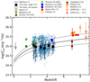 |
Fig. 3.
|


We show the relations between  and MUV and between
  and the UV slope β in Fig. 4 and color-code each object according to the relevant redshift. We find mild but significant correlations in both cases. The ionizing efficiency increases at fainter MUV (rs = 0.23) from 24.8 at MUV ∼ −21.4 to ∼25.2 at MUV ∼ −18.8. Similarly,
  increases at a decreasing UV slope β (rs = −0.23). These trends are weaker, but still significant according to the Spearman correlation test when only objects with log(Mstar/M⊙) > 9.5 are considered. The relation with the UV slope is nearly flat, with the possible exception of objects at extremely blue β < −3. No clear redshift-dependent effect is evident in the diagrams described above. Objects at z ∼ 2 − 5 populate the entire observed range.
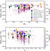 |
Fig. 4.
|

The relation between the ionizing efficiency and the EW of the UV emission lines is shown in Fig. 5. There is a robust significant trend of increasing  at increasing EW(Lyα) (rs = 0.42) with an average log(
 /Hz erg−1) > 25 at EW > 50 Å. Instead, the correlations between
  and other emission lines are much milder. According to the Spearman test, the correlations between
  and the EW of both CIII]λ1909 (rs = 0.22) and OIII]λ1666 (rs = 0.27) are significant when objects in the full sample with a line detection are considered, but only the latter remains significant (with rs = 0.36) for objects with log(Mstar/M⊙) > 9.5. The positive correlation with EW(CIII]λ1909) is likely driven by the few objects with CIII]λ1909 with an EW > 20 Å and an average log(
 /Hz erg−1)∼25.2. In turn, no significant correlation is found between
  and the EW of HeIIλ1640.
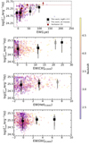 |
Fig. 5. Same as Fig. 4 but for the EWs of Lyα, CIII], HeII, and OIII], from top to bottom. Negative values on single objects are due to absorption in the case of Lyα and to measurement noise on galaxies with EW ∼ 0 for the other lines. The |

4.2. Dependence of  on the physical parameters
In Fig. 6 we show the relation between  and physical properties for the VANDELS sample. We find a significant trend of increasing average ionizing efficiency at decreasing mass (rs = −0.54). log(
 /Hz erg−1) evolves from ∼24.8 at log(Mstar/M⊙) > 11 to ≳25 at log(Mstar/M⊙) < 10. A large scatter is found on the
  –SFR plane, but there is a clear prevalence of objects with high
  at SFR > 100 M⊙ yr−1, and the Spearman test indicates a significant correlation for the full sample (rs = 0.16) and the high-mass sample (rs = 0.38).
The most evident correlation is found between  and sSFR, with a monotonic increase from log(
 /Hz erg−1) ∼24.5 at log(sSFR) ∼ −9.5 yr−1 to ∼25.5 at log(sSFR) ∼ −7.5 yr−1. Most importantly, the sSFR–
 relation has a low scatter, which is at variance with the other relations discussed here, and it shows no evidence for multimodal distributions. The correlation is significant according to the Spearman test and shows little dependence on mass. The full sample and the log(Mstar/M⊙) > 9.5 sample have rs = 0.79 and rs = 0.68, respectively, and the average values as a function of sSFR are similar. The correlation is particularly evident when the VANDELS sample is analyzed in the Mstar–SFR plane (Fig. 7). Objects above the main sequence of star formation have higher than average
  , and vice versa, low
  is found in galaxies whose SFR is lower than the typical value at their stellar mass.
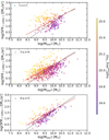 |
Fig. 7. VANDELS sample on the SFR vs. Mstar plane. Each object is color-coded according to the relevant |

The ionizing efficiency also shows a significant increase in compact star-forming objects (rs = 0.35 − 0.38 for the full and the high-mass samples). The galaxies with ΣSFR > 10 M⊙ yr−1 kpc−2 have log( /Hz erg−1) > 25 with very few exceptions, and these high efficiencies are prevalent at ΣSFR > 1 M⊙ yr−1 kpc−2.
Building on the results discussed above, we searched for an equation to provide an estimate of  on the basis of the physical properties of the galaxies. To do this, we carried out a fully data-driven power regression analysis to evaluate equations combining the measured parameters following the approach described in Mascia et al. (2023a). A regularized minimization of the sum of the root mean squared error (RMSE) and of the mean absolute error (MAE), computed between the values provided by each equation and the dataset, yields the following regression as the best description of our dataset:

The coefficients and corresponding uncertainties were estimated by repeating the minimization process 1000 times with a bootstrap approach, in which 10% of the sample was randomly removed in every iteration:
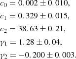
The power-law model presented above yields an RMSE = 0.2 and an MAE = 0.15. This particular model, which is a function of the SFR and the stellar mass, was selected as the best alternative to minimize the error. This is consistent from a physical perspective with the clear correlation between the sSFR and  .
.
4.3. Comparison with previous results
The relation between  and redshift as well as its correlation with observed properties was explored in several recent works. In Fig. 3 we compare our estimates to previous measurements of
  from representative samples of star-forming galaxies at different redshifts. The average ionizing efficiency as a function of redshift computed on the entire VANDELS sample (empty black squares in Fig. 3) agrees with the
  –redshift relation by Matthee et al. (2017), while our log(Mstar/M⊙) > 9.5 sample (filled black squares) lies below their average. The average
  value measured by Nakajima et al. (2018) on a composite of star-forming galaxies at z ∼ 2 − 4 is higher than both the VANDELS and the Matthee et al. (2017) averages, but the difference can be partly due to their use of BPASS models, which include binary stellar populations with a 300 M⊙ upper mass cutoff of the IMF (Stanway et al. 2016).
Our objects also show lower average  than the samples by Shivaei et al. (2018) and Bouwens et al. (2016) at z ∼ 2 and z ∼ 4.5, respectively, in particular when compared to estimates based on a Small Magellanic Cloud (SMC) extinction law. Similarly, the
  − MUV, and
  − β relations in our sample have lower average values than those from the literature (Bouwens et al. 2016; Lam et al. 2019; Emami et al. 2020; Prieto-Lyon et al. 2023), although, as discussed in Sect. 4.1, both relations appear to be bimodal, and the locus of VANDELS objects with a higher ionizing efficiency includes all observed values from the literature. Our average
  values at MUV ≲ −20 and as a function of UV slope agree better with the measurements by Shivaei et al. (2018) based on the Calzetti et al. (2000) attenuation law.
Most importantly, a good agreement is found with the  − Mstar relations by Shivaei et al. (2018; based on Calzetti attenuation), Lam et al. (2019), and Emami et al. (2020) at log(Mstar/M⊙) < 10. At higher stellar masses, the VANDELS sample has a lower average ionizing efficiency than the 1.4 ≤ z ≤ 3.8 sample by Shivaei et al. (2018), whose
  − Mstar relation bends and increases again at very high masses. Considering the apparent bimodal structure of the
  − Mstar distribution and the low number of VANDELS objects in the most massive bin shown in Fig. 6, we can explain the difference at high masses by sample variance or by the different analyzed redshift range.
The comparison with previous works on the  − Mstar plane is extremely important to explain the discrepancies described above. The tendency towards lower
  values than in Bouwens et al. (2016) and other works is most likely explained by the different mass distributions in the two samples, with an average log(Mstar/M⊙)∼9.2 in their sample compared to ∼9.9 in VANDELS. This is also evident for the comparison with the results by Lam et al. (2019), whose sample extends to log(Mstar/M⊙) < 8. The sample by Prieto-Lyon et al. (2023) includes Lyα-detected objects with an average MUV ∼ −18 that are most likely much less massive than the VANDELS galaxies. Interestingly, the average values for the full VANDELS sample agree better with those from Lam et al. (2019) and Emami et al. (2020) on the
  − β plane as well. The lower average
  values in our sample likely arise becuase high-mass objects are older and more metal rich.
The  –EW(Lyα) relation in our data is also consistent with previous findings for z ∼ 5 LAEs by Harikane et al. (2018), but the average values are ∼0.2 dex lower at fixed EW. This discrepancy can also likely be explained by the higher average stellar mass of our sample of bright LBGs, which means that they are most likely older and more enriched than the log(Mstar/M⊙)∼8 − 9 of the z ∼ 5 narrowband-selected LAEs. We cannot exclude that the redshift evolution in the properties of Lyα emitters may play a role, however.
A correlation between  and sSFR was previously found by Izotov et al. (2021) for CSFGs at z < 1. They constrained a clear trend between
  and the quantity SFR−0.9 × Mstar, which is monotonically correlated with the gas-phase metallicity according to the fundamental mass–metallicity relation (Mannucci et al. 2010). When we recast our
  –sSFR relation in this plane (not shown here), we find a consistent trend, but with a lower scatter and a slightly lower normalization (∼0.1 dex), which is again possibly due to the lack of low-mass galaxies in the VANDELS sample.
5. Summary and discussion
We have used the spectrophotometric fitting code BEAGLE to measure the ionizing efficiency and other physical parameters for a sample of 1174 galaxies with secure spectroscopic redshifts at z ∼ 2 − 5 in the VANDELS survey. The sample comprises mostly bright (MUV < −20) massive galaxies, with a high completeness at log(Mstar/M⊙) > 9.5. The measurement of the physical properties exploited the availability of deep multiband photometry in the VANDELS area and the measurement of emission lines in the UV rest-frame range (Lyα, CIII]λ1909, HeIIλ1640, and OIII]λ1666). The spectrophotometric approach adopted here is the same as was used for galaxies in the EoR (e.g., Stark et al. 2015b; Castellano et al. 2022b) and provides a useful reference to infer  from the observed properties of very high-redshift galaxies. We explored the correlation between ionizing efficiency and galaxy properties by evaluating their statistical significance on the basis of Spearman (1904) rank coefficients, which are summarised in Fig. 8 both for the entire sample and the high-mass sample.
 |
Fig. 8. Spearman rank coefficients for the correlation between |

We find no evolution of  with redshift within the probed range and a mild increase in the ionizing efficiency at fainter MUV and bluer UV slopes. The most significant correlations are found with respect to EW(Lyα), stellar mass, ΣSFR, and specific SFR. The latter relation is particularly interesting: it is apparently unimodal, with a remarkably low scatter, and it is significant both in the full sample and in the log(Mstar/M⊙) > 9.5 sample. As a result, the objects above the main sequence of star formation consistently have higher than average
  , and vice versa, low
  is found in galaxies whose SFR is lower than the typical value at their stellar mass. Our results can be clearly visualized by studying at the differences between the distributions for objects with high (log(
 /Hz erg−1) > 25.2) and low efficiency in our high-mass subsample (Fig. 9). The probability density distributions of sSFR, SFR, and ΣSFR are clearly different. A difference is also apparent in the high-EW tail of the EW(Lyα) distribution, while the MUV and UV slope distributions are very similar for the two samples. According to a two-sided Kolmogorov–Smirnov test (Hodges 1958), the null hypothesis that the two samples are drawn from the same parent distribution has p < 0.01 for sSFR, SFR, and ΣSFR, and just a slightly higher significance (p ∼ 0.03) in the EW(Lyα) case. The subsamples of objects with low and high
  are statistically equivalent (p > 0.15) as far as MUV and β are concerned. An inverse correlation between metallicity and
  provides a possible physical explanation for the observed relations (Yung et al. 2020). In this scenario, the inverse trend of
  with stellar mass is a natural consequence of the underlying mass-metallicity relation (e.g., Calabrò et al. 2021; Curti et al. 2023), while objects with high ΣSFR and galaxies above the main sequence have an enhanced ionizing efficiency due to ongoing star formation episodes from low-metallicity gas (Amorín et al. 2017). The increase in the EW of CIII]λ1909 and OIII]λ1666 at low gas-phase metallicity (e.g., Stark et al. 2014) also explains the correlations we found between these collisionally excited emission lines and
  . In turn, the lack of a correlation with HeIIλ1640 is consistent with the findings by Saxena et al. (2020) that high-redshift HeII emitters and nonemitters have a comparable metallicity. Additional poorly known mechanisms such as X-ray binaries or stripped stars are needed to fully account for the emission rate of HeII ionizing photons.
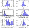 |
Fig. 9. Probability density distributions of MUV, the UV slope, the EW(Lyα), the SFR, the ΣSFR, and sSFR from top left to bottom right for objects with |


These findings have important consequences for the investigation of the epoch of reionization. There are intriguing similarities between our results and the observed trends between escape fraction and galaxy properties. The escape fraction has been found to be positively correlated with EW(Lyα), sSFR, and ΣSFR and to be anticorrelated with stellar mass and metallicity (e.g., Pahl et al. 2021; Flury et al. 2022; Begley et al. 2022). While differences remain (e.g., the anticorrelation with UV slope is more evident for fesc than for  ), the emerging scenario indicates that compact high sSFR galaxies are efficient sources of ionizing photons that are leaked into the IGM through density-bounded regions or through channels carved by star formation feedback (Gazagnes et al. 2020). In this respect, the increase in sSFR that has been found at high-redshift (e.g., Stark et al. 2013; Castellano et al. 2017; Topping et al. 2022) suggests an increase in both ionizing efficiency and in the availability of moderate escape fractions of ionizing photons to keep the IGM ionized (Chisholm et al. 2022; Lin et al. 2023; Mascia et al. 2023a). Finally, both the spectrophotometric analysis of the UV rest-frame range and the availability of sSFR and ΣSFR as proxies for
  can be of fundamental importance to determine the role at the onset of reionization of the galaxy populations that are being discovered by JWST NIRCam at z ≳ 10, where rest-frame optical emission lines fall outside the spectral range observable with NIRSpec (e.g., Castellano et al. 2022a, 2023; Naidu et al. 2022; Harikane et al. 2023; Curtis-Lake et al. 2023). The fitting equation presented in Sect. 4.2 to estimate
  from SFR and Mstar provides a first step in this direction. Forthcoming JWST spectroscopic surveys will allow us to extend the present analysis to higher redshifts and lower masses in order to derive robust estimators of the ionizing efficiency of the very first galaxies.
The data release is available at http://vandels.inaf.it/db and https://www.eso.org/qi/
Acknowledgments
We thank the referee for the detailed and constructive comments. We thank Irene Shivaei for kindly providing tabulated data from Shivaei et al. (2018). The present paper exploits Cineca computing resources obtained under projects INA20_C6T27, and INA20_C7B36. We acknowledge the computing centre of Cineca and INAF, under the coordination of the “Accordo Quadro MoU per lo svolgimento di attivitá congiunta di ricerca Nuove frontiere in Astrofisica: HPC e Data Exploration di nuova generazione”, for the availability of computing resources and support. MC and PS acknowledge support from INAF Minigrant “Reionization and fundamental cosmology with high-redshift galaxies”.
References
- Amorín, R., Fontana, A., Pérez-Montero, E., et al. 2017, Nat. Astron., 1, 0052 [Google Scholar]
- Begley, R., Cullen, F., McLure, R. J., et al. 2022, MNRAS, 513, 3510 [NASA ADS] [CrossRef] [Google Scholar]
- Borghi, N., Moresco, M., Cimatti, A., et al. 2022, ApJ, 927, 164 [NASA ADS] [CrossRef] [Google Scholar]
- Bouwens, R. J., Smit, R., Labbé, I., et al. 2016, ApJ, 831, 176 [Google Scholar]
- Bouwens, R. J., Oesch, P. A., Stefanon, M., et al. 2021, AJ, 162, 47 [NASA ADS] [CrossRef] [Google Scholar]
- Bruzual, G., & Charlot, S. 2003, MNRAS, 344, 1000 [NASA ADS] [CrossRef] [Google Scholar]
- Calabrò, A., Castellano, M., Pentericci, L., et al. 2021, A&A, 646, A39 [EDP Sciences] [Google Scholar]
- Calabrò, A., Pentericci, L., Talia, M., et al. 2022, A&A, 667, A117 [NASA ADS] [CrossRef] [EDP Sciences] [Google Scholar]
- Calzetti, D., Armus, L., Bohlin, R. C., et al. 2000, ApJ, 533, 682 [NASA ADS] [CrossRef] [Google Scholar]
- Cardiel, N., Gorgas, J., Cenarro, J., & Gonzalez, J. J. 1998, A&AS, 127, 597 [NASA ADS] [CrossRef] [EDP Sciences] [Google Scholar]
- Carnall, A. C., Leja, J., Johnson, B. D., et al. 2019, ApJ, 873, 44 [Google Scholar]
- Castellano, M., Fontana, A., Paris, D., et al. 2010, A&A, 524, A28 [NASA ADS] [CrossRef] [EDP Sciences] [Google Scholar]
- Castellano, M., Pentericci, L., Fontana, A., et al. 2017, ApJ, 839, 73 [NASA ADS] [CrossRef] [Google Scholar]
- Castellano, M., Fontana, A., Treu, T., et al. 2022a, ApJ, 938, L15 [NASA ADS] [CrossRef] [Google Scholar]
- Castellano, M., Pentericci, L., Cupani, G., et al. 2022b, A&A, 662, A115 [NASA ADS] [CrossRef] [EDP Sciences] [Google Scholar]
- Castellano, M., Fontana, A., Treu, T., et al. 2023, ApJ, 948, L14 [NASA ADS] [CrossRef] [Google Scholar]
- Ceverino, D., Klessen, R. S., & Glover, S. C. O. 2019, MNRAS, 484, 1366 [NASA ADS] [CrossRef] [Google Scholar]
- Chabrier, G. 2003, PASP, 115, 763 [Google Scholar]
- Charlot, S., & Fall, S. M. 2000, ApJ, 539, 718 [Google Scholar]
- Chevallard, J., & Charlot, S. 2016, MNRAS, 462, 1415 [NASA ADS] [CrossRef] [Google Scholar]
- Chevallard, J., Charlot, S., Wandelt, B., & Wild, V. 2013, MNRAS, 432, 2061 [CrossRef] [Google Scholar]
- Chevallard, J., Charlot, S., Senchyna, P., et al. 2018, MNRAS, 479, 3264 [Google Scholar]
- Chisholm, J., Rigby, J. R., Bayliss, M., et al. 2019, ApJ, 882, 182 [Google Scholar]
- Chisholm, J., Saldana-Lopez, A., Flury, S., et al. 2022, MNRAS, 517, 5104 [CrossRef] [Google Scholar]
- Ciesla, L., Elbaz, D., & Fensch, J. 2017, A&A, 608, A41 [NASA ADS] [CrossRef] [EDP Sciences] [Google Scholar]
- Cullen, F., Shapley, A. E., McLure, R. J., et al. 2021, MNRAS, 505, 903 [CrossRef] [Google Scholar]
- Curti, M., Maiolino, R., Carniani, S., et al. 2023, A&A, submitted [arXiv:2304.08516] [Google Scholar]
- Curtis-Lake, E., Carniani, S., Cameron, A., et al. 2023, Nat. Astron., 7, 622 [NASA ADS] [CrossRef] [Google Scholar]
- Dayal, P., & Ferrara, A. 2018, Phys. Rep., 780, 1 [Google Scholar]
- Domínguez, A., Siana, B., Henry, A. L., et al. 2013, ApJ, 763, 145 [CrossRef] [Google Scholar]
- Duncan, K., & Conselice, C. J. 2015, MNRAS, 451, 2030 [NASA ADS] [CrossRef] [Google Scholar]
- Emami, N., Siana, B., Alavi, A., et al. 2020, ApJ, 895, 116 [NASA ADS] [CrossRef] [Google Scholar]
- Endsley, R., Stark, D. P., Charlot, S., et al. 2021a, MNRAS, 502, 6044 [NASA ADS] [CrossRef] [Google Scholar]
- Endsley, R., Stark, D. P., Chevallard, J., & Charlot, S. 2021b, MNRAS, 500, 5229 [Google Scholar]
- Endsley, R., Stark, D. P., Whitler, L., et al. 2023, MNRAS, in press, https://doi.org/10.1093/mnras/stad1919 [Google Scholar]
- Faisst, A. L., Capak, P. L., Emami, N., Tacchella, S., & Larson, K. L. 2019, ApJ, 884, 133 [NASA ADS] [CrossRef] [Google Scholar]
- Feltre, A., Charlot, S., & Gutkin, J. 2016, MNRAS, 456, 3354 [Google Scholar]
- Ferland, G. J., Porter, R. L., van Hoof, P. A. M., et al. 2013, Rev. Mex. Astron. Astrofís., 49, 137 [Google Scholar]
- Feroz, F., & Hobson, M. P. 2008, MNRAS, 384, 449 [NASA ADS] [CrossRef] [Google Scholar]
- Flury, S. R., Jaskot, A. E., Ferguson, H. C., et al. 2022, ApJS, 260, 1 [NASA ADS] [CrossRef] [Google Scholar]
- Fontana, A., Dunlop, J. S., Paris, D., et al. 2014, A&A, 570, A11 [NASA ADS] [CrossRef] [EDP Sciences] [Google Scholar]
- Fujimoto, S., Arrabal Haro, P., Dickinson, M., et al. 2023, ApJ, 949, L25 [NASA ADS] [CrossRef] [Google Scholar]
- Galametz, A., Grazian, A., Fontana, A., et al. 2013, ApJS, 206, 10 [Google Scholar]
- Garilli, B., Fumana, M., Franzetti, P., et al. 2010, PASP, 122, 827 [Google Scholar]
- Garilli, B., McLure, R., Pentericci, L., et al. 2021, A&A, 647, A150 [NASA ADS] [CrossRef] [EDP Sciences] [Google Scholar]
- Gazagnes, S., Chisholm, J., Schaerer, D., Verhamme, A., & Izotov, Y. 2020, A&A, 639, A85 [NASA ADS] [CrossRef] [EDP Sciences] [Google Scholar]
- Grazian, A., Giallongo, E., Gerbasi, R., et al. 2016, A&A, 585, A48 [NASA ADS] [CrossRef] [EDP Sciences] [Google Scholar]
- Grogin, N. A., Kocevski, D. D., Faber, S. M., et al. 2011, ApJS, 197, 35 [NASA ADS] [CrossRef] [Google Scholar]
- Guo, Y., Ferguson, H. C., Giavalisco, M., et al. 2013, ApJS, 207, 24 [NASA ADS] [CrossRef] [Google Scholar]
- Gutkin, J., Charlot, S., & Bruzual, G. 2016, MNRAS, 462, 1757 [Google Scholar]
- Harikane, Y., Ouchi, M., Shibuya, T., et al. 2018, ApJ, 859, 84 [NASA ADS] [CrossRef] [Google Scholar]
- Harikane, Y., Ouchi, M., Oguri, M., et al. 2023, ApJS, 265, 5 [NASA ADS] [CrossRef] [Google Scholar]
- Hodges, J., Jr 1958, Arkiv för Matematik, 3, 469 [CrossRef] [Google Scholar]
- Izotov, Y. I., Guseva, N. G., Fricke, K. J., Henkel, C., & Schaerer, D. 2017, MNRAS, 467, 4118 [NASA ADS] [CrossRef] [Google Scholar]
- Izotov, Y. I., Schaerer, D., Worseck, G., et al. 2018a, MNRAS, 474, 4514 [Google Scholar]
- Izotov, Y. I., Worseck, G., Schaerer, D., et al. 2018b, MNRAS, 478, 4851 [Google Scholar]
- Izotov, Y. I., Guseva, N. G., Fricke, K. J., et al. 2021, A&A, 646, A138 [NASA ADS] [CrossRef] [EDP Sciences] [Google Scholar]
- Kennicutt, R. C., Jr 1998, ARA&A, 36, 189 [NASA ADS] [CrossRef] [Google Scholar]
- Kennicutt, R. C., & Evans, N. J. 2012, ARA&A, 50, 531 [NASA ADS] [CrossRef] [Google Scholar]
- Kocevski, D. D., Hasinger, G., Brightman, M., et al. 2018, ApJS, 236, 48 [CrossRef] [Google Scholar]
- Koekemoer, A. M., Faber, S. M., Ferguson, H. C., et al. 2011, ApJS, 197, 36 [NASA ADS] [CrossRef] [Google Scholar]
- Lam, D., Bouwens, R. J., Labbé, I., et al. 2019, A&A, 627, A164 [NASA ADS] [CrossRef] [EDP Sciences] [Google Scholar]
- Leitherer, C., & Heckman, T. M. 1995, ApJS, 96, 9 [NASA ADS] [CrossRef] [Google Scholar]
- Leitherer, C., Tremonti, C. A., Heckman, T. M., & Calzetti, D. 2011, AJ, 141, 37 [NASA ADS] [CrossRef] [Google Scholar]
- Lin, Y. H., Scarlata, C., Williams, H., et al. 2023, ArXiv e-prints [arXiv:2303.04572] [Google Scholar]
- Luo, B., Brandt, W. N., Xue, Y. Q., et al. 2017, ApJS, 228, 2 [Google Scholar]
- Ma, X., Hopkins, P. F., Kasen, D., et al. 2016, MNRAS, 459, 3614 [Google Scholar]
- Mannucci, F., Cresci, G., Maiolino, R., Marconi, A., & Gnerucci, A. 2010, MNRAS, 408, 2115 [NASA ADS] [CrossRef] [Google Scholar]
- Maraston, C., Nieves Colmenárez, L., Bender, R., & Thomas, D. 2009, A&A, 493, 425 [NASA ADS] [CrossRef] [EDP Sciences] [Google Scholar]
- Marchi, F., Pentericci, L., Guaita, L., et al. 2017, A&A, 601, A73 [NASA ADS] [CrossRef] [EDP Sciences] [Google Scholar]
- Mascia, S., Pentericci, L., Calabrò, A., et al. 2023a, A&A, 672, A155 [NASA ADS] [CrossRef] [EDP Sciences] [Google Scholar]
- Mascia, S., Pentericci, L., Saxena, A., et al. 2023b, A&A, 674, A221 [NASA ADS] [CrossRef] [EDP Sciences] [Google Scholar]
- Matthee, J., Sobral, D., Best, P., et al. 2017, MNRAS, 465, 3637 [NASA ADS] [CrossRef] [Google Scholar]
- McLure, R. J., Pentericci, L., Cimatti, A., et al. 2018, MNRAS, 479, 25 [NASA ADS] [Google Scholar]
- Naidu, R. P., Oesch, P. A., van Dokkum, P., et al. 2022, ApJ, 940, L14 [NASA ADS] [CrossRef] [Google Scholar]
- Nakajima, K., Ellis, R. S., Iwata, I., et al. 2016, ApJ, 831, L9 [Google Scholar]
- Nakajima, K., Schaerer, D., Le Fèvre, O., et al. 2018, A&A, 612, A94 [NASA ADS] [CrossRef] [EDP Sciences] [Google Scholar]
- Oke, J. B., & Gunn, J. E. 1983, ApJ, 266, 713 [NASA ADS] [CrossRef] [Google Scholar]
- Pahl, A. J., Shapley, A., Steidel, C. C., Chen, Y., & Reddy, N. A. 2021, MNRAS, 505, 2447 [NASA ADS] [CrossRef] [Google Scholar]
- Pei, Y. C. 1992, ApJ, 395, 130 [Google Scholar]
- Pentericci, L., McLure, R. J., Garilli, B., et al. 2018, A&A, 616, A174 [NASA ADS] [CrossRef] [EDP Sciences] [Google Scholar]
- Prieto-Lyon, G., Strait, V., Mason, C. A., et al. 2023, A&A, 672, A186 [NASA ADS] [CrossRef] [EDP Sciences] [Google Scholar]
- Reddy, N. A., Shapley, A. E., Sanders, R. L., et al. 2018, ApJ, 869, 92 [NASA ADS] [CrossRef] [Google Scholar]
- Ribeiro, B., Le Fèvre, O., Tasca, L. A. M., et al. 2016, A&A, 593, A22 [NASA ADS] [CrossRef] [EDP Sciences] [Google Scholar]
- Robertson, B. E. 2022, ARA&A, 60, 121 [NASA ADS] [CrossRef] [Google Scholar]
- Robertson, B. E., Furlanetto, S. R., Schneider, E., et al. 2013, ApJ, 768, 71 [Google Scholar]
- Santini, P., Ferguson, H. C., Fontana, A., et al. 2015, ApJ, 801, 97 [Google Scholar]
- Saxena, A., Pentericci, L., Mirabelli, M., et al. 2020, A&A, 636, A47 [NASA ADS] [CrossRef] [EDP Sciences] [Google Scholar]
- Schaerer, D., Izotov, Y. I., Verhamme, A., et al. 2016, A&A, 591, L8 [NASA ADS] [CrossRef] [EDP Sciences] [Google Scholar]
- Schaerer, D., Marques-Chaves, R., Barrufet, L., et al. 2022, A&A, 665, L4 [NASA ADS] [CrossRef] [EDP Sciences] [Google Scholar]
- Schreiber, C., Pannella, M., Elbaz, D., et al. 2015, A&A, 575, A74 [NASA ADS] [CrossRef] [EDP Sciences] [Google Scholar]
- Schreiber, C., Glazebrook, K., Nanayakkara, T., et al. 2018, A&A, 618, A85 [NASA ADS] [CrossRef] [EDP Sciences] [Google Scholar]
- Shivaei, I., Reddy, N. A., Siana, B., et al. 2018, ApJ, 855, 42 [Google Scholar]
- Sobral, D., & Matthee, J. 2019, A&A, 623, A157 [NASA ADS] [CrossRef] [EDP Sciences] [Google Scholar]
- Speagle, J. S., Steinhardt, C. L., Capak, P. L., & Silverman, J. D. 2014, ApJS, 214, 15 [Google Scholar]
- Spearman, C. 1904, Am. J. Psychol., 15, 201 [CrossRef] [Google Scholar]
- Stanway, E. R., Eldridge, J. J., & Becker, G. D. 2016, MNRAS, 456, 485 [NASA ADS] [CrossRef] [Google Scholar]
- Stark, D. P., Schenker, M. A., Ellis, R., et al. 2013, ApJ, 763, 129 [Google Scholar]
- Stark, D. P., Richard, J., Siana, B., et al. 2014, MNRAS, 445, 3200 [NASA ADS] [CrossRef] [Google Scholar]
- Stark, D. P., Richard, J., Charlot, S., et al. 2015a, MNRAS, 450, 1846 [NASA ADS] [CrossRef] [Google Scholar]
- Stark, D. P., Walth, G., Charlot, S., et al. 2015b, MNRAS, 454, 1393 [Google Scholar]
- Stark, D. P., Ellis, R. S., Charlot, S., et al. 2017, MNRAS, 464, 469 [NASA ADS] [CrossRef] [Google Scholar]
- Stefanon, M., Bouwens, R. J., Illingworth, G. D., et al. 2022, ApJ, 935, 94 [NASA ADS] [CrossRef] [Google Scholar]
- Steidel, C. C., Bogosavljević, M., Shapley, A. E., et al. 2018, ApJ, 869, 123 [Google Scholar]
- Tang, M., Stark, D. P., Chevallard, J., & Charlot, S. 2019, MNRAS, 489, 2572 [NASA ADS] [CrossRef] [Google Scholar]
- Topping, M. W., Stark, D. P., Endsley, R., et al. 2022, MNRAS, 516, 975 [NASA ADS] [CrossRef] [Google Scholar]
- van der Wel, A., Noeske, K., Bezanson, R., et al. 2016, ApJS, 223, 29 [Google Scholar]
- Vanzella, E., de Barros, S., Vasei, K., et al. 2016, ApJ, 825, 41 [NASA ADS] [CrossRef] [Google Scholar]
- Vidal-García, A., Charlot, S., Bruzual, G., & Hubeny, I. 2017, MNRAS, 470, 3532 [Google Scholar]
- Wilkins, S. M., Feng, Y., Di-Matteo, T., et al. 2016, MNRAS, 458, L6 [NASA ADS] [CrossRef] [Google Scholar]
- Yung, L. Y. A., Somerville, R. S., Popping, G., & Finkelstein, S. L. 2020, MNRAS, 494, 1002 [NASA ADS] [CrossRef] [Google Scholar]
Appendix A: Average ionizing efficiency as a function of the observed and physical properties
We report in Tab. A.1 and A.2 the average and standard deviation of the ionizing efficiency of the VANDELS objects with log(Mstar/M⊙) > 9.5 as a function of the observed and physical properties. The statistics as a function of mass on the full sample is included in Tab. A.2 for reference.
Ionizing efficiency as a function of the observed properties
Ionizing efficiency as a function of the physical properties
All Tables
All Figures
|
Fig. 1. Main properties of the VANDELS sample (black) and of the objects with log(Mstar/M⊙) > 9.5 (red). The spectroscopic redshifts are from VANDELS DR4, stellar masses (Mstar) have been estimated with BEAGLE as discussed in Sect. 3, and the UV magnitudes (MUV) and slopes (β) have been measured from the observed photometry (Sect. 2.1). The green continuous line in the top right panel shows the Mstar distribution for all CANDELS objects at z = 2 − 5 in UDS and GOODS-South from Santini et al. (2015), scaled by a factor of 4 to take the target sampling of the spectroscopic survey into account. |
| In the text | |
|
Fig. 2. Tests of the accuracy of the BEAGLE SED-fitting results. Top: comparison between the BEAGLE best-fit flux and the observed flux of the lines used in the spectrophotometric fitting. Bottom: comparison between the |
| In the text | |
|
Fig. 3.
|
| In the text | |
|
Fig. 4.
|
| In the text | |
|
Fig. 5. Same as Fig. 4 but for the EWs of Lyα, CIII], HeII, and OIII], from top to bottom. Negative values on single objects are due to absorption in the case of Lyα and to measurement noise on galaxies with EW ∼ 0 for the other lines. The |
| In the text | |
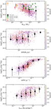 |
Fig. 6. Same as Fig. 4 but for Mstar, SFR, sSFR, and ΣSFR, from top to bottom. |
| In the text | |
|
Fig. 7. VANDELS sample on the SFR vs. Mstar plane. Each object is color-coded according to the relevant |
| In the text | |
|
Fig. 8. Spearman rank coefficients for the correlation between |
| In the text | |
|
Fig. 9. Probability density distributions of MUV, the UV slope, the EW(Lyα), the SFR, the ΣSFR, and sSFR from top left to bottom right for objects with |
| In the text | |
Current usage metrics show cumulative count of Article Views (full-text article views including HTML views, PDF and ePub downloads, according to the available data) and Abstracts Views on Vision4Press platform.
Data correspond to usage on the plateform after 2015. The current usage metrics is available 48-96 hours after online publication and is updated daily on week days.
Initial download of the metrics may take a while.