| Issue |
A&A
Volume 698, June 2025
|
|
|---|---|---|
| Article Number | A314 | |
| Number of page(s) | 24 | |
| Section | Planets, planetary systems, and small bodies | |
| DOI | https://doi.org/10.1051/0004-6361/202453241 | |
| Published online | 27 June 2025 | |
Time-resolved absorption of six chemical species with MAROON-X points to a strong drag in the ultra-hot Jupiter TOI-1518 b
1
Laboratoire Lagrange, Université Côte d’Azur, Observatoire de la Côte d’Azur, CNRS,
Nice,
France
2
Institut Trottier de Recherche sur les Exoplanètes, Université de Montréal, Montréal,
Québec
H3T 1J4,
Canada
3
Tsung-Dao Lee Institute, Shanghai Jiao Tong University,
520 Shengrong Road,
Shanghai,
PR China
4
School of Physics and Astronomy, Shanghai Jiao Tong University,
800 Dongchuan Road,
Shanghai,
PR China
5
Institut d’astrophysique de Paris, UMR7095 CNRS, Université Pierre & Marie Curie,
98bis boulevard Arago,
75014
Paris,
France
6
Lund Observatory, Department of Astronomy and Theoretical Physics, Department of Physics, Lund University,
Lund,
Sweden
7
European Southern Observatory,
Alonso de Córdova 3107,
Vitacura, Región Metropolitana,
Chile
8
Department of Astronomy & Astrophysics, University of Chicago,
Chicago,
IL
60637,
USA
9
Observatoire de Haute-Provence, CNRS, Université d’Aix-Marseille,
04870
Saint-Michel-l’Observatoire,
France
10
School of Earth and Space Exploration, Arizona State University,
Tempe,
AZ
85281,
USA
11
Center for Space and Habitability, University of Bern,
Gesellschaftsstrasse 6,
3012
Bern,
Switzerland
12
Observatoire astronomique de l’Université de Genève,
51 chemin Pegasi 1290 Versoix,
Switzerland
13
Gemini Observatory/NSF NOIRLab,
670 N. A’ohoku Place,
Hilo,
HI
96720,
USA
14
Univ. Grenoble Alpes, CNRS, IPAG,
414 rue de la Piscine,
38400
St-Martin d’Hères,
France
15
Department of Physics, University of Turin,
Via Pietro Giuria 1,
10125
Turin,
Italy
16
INAF – Osservatorio Astrofisico di Torino,
Via Osservatorio 20,
10025
Pino Torinese,
Italy
17
Anton Pannekoek Institute of Astronomy, University of Amsterdam,
Amsterdam,
The Netherlands
18
Department of Physics, University of Warwick,
Coventry
CV4 7AL,
UK
19
Centre for Exoplanets and Habitability, University of Warwick,
Gibbet Hill Road,
Coventry
CV4 7AL,
UK
20
Atmospheric, Oceanic, and Planetary Physics, Department of Physics, University of Oxford,
Parks Rd,
Oxford
OX1 3PU,
UK
21
Université de Toulouse, CNRS, IRAP,
14 avenue Belin,
31400
Toulouse,
France
22
LESIA, Observatoire de Paris, Univ PSL, CNRS, Sorbonne Univ, Univ de Paris,
5 place Jules Janssen,
92195
Meudon,
France
23
INAF-Osservatorio Astrofisico di Arcetri Largo Enrico Fermi,
Florence,
Italy
24
Department of Astronomy, University of Michigan,
Ann Arbor,
MI
48109,
USA
25
Steward Observatory, University of Arizona,
Tucson,
AZ,
USA
26
International Center for Advanced Studies (ICAS) and ICIFI (CONICET), ECyT-UNSAM,
Campus Miguelete, 25 de Mayo y Francia,
1650
Buenos Aires,
Argentina
★ Corresponding author: This email address is being protected from spambots. You need JavaScript enabled to view it.
Received:
30
November
2024
Accepted:
8
April
2025
Abstract
Context. Wind dynamics play a pivotal role in governing transport processes within planetary atmospheres, influencing atmospheric chemistry, cloud formation, and the overall energy budget. Understanding the strength and patterns of winds is crucial for comprehensive insights into the physics of ultra-hot-Jupiter atmospheres. Current research has proposed different mechanisms that limit wind speeds in these atmospheres.
Aims. This study focuses on unraveling the wind dynamics and the chemical composition in the atmosphere of the ultra-hot Jupiter TOI-1518 b.
Methods. Two transit observations using the high-resolution (Rλ ∼ 85 000) optical (spectral coverage between 490 and 920 nm) spectrograph MAROON-X were obtained and analyzed to explore the chemical composition and wind dynamics using the cross-correlation techniques, global circulation models (GCMs), and atmospheric retrieval.
Results. We report the detection of 14 species in the atmosphere of TOI-1518 b through cross-correlation analysis. VO was detected only with the new HyVO line list, whereas TiO was not detected. Additionally, we measured the time-varying cross-correlation trails for six different species, compared them with predictions from GCMs, and conclude that a strong drag is slowing the winds in TOI-1518 b’s atmosphere (τdrag ≈ 103−104 s). We find that the trails are species dependent. Fe+ favors stronger drag than Fe, which we interpret as a sign of magnetic effects being responsible for the observed strong drag. Furthermore, we show that Ca+ probes layers above the Roche lobe, leading to a qualitatively different trail than the other species. Finally, We used a retrieval analysis to further characterize the abundances of the different species detected. Our analysis is refined thanks to the updated planetary mass of 1.83 ± 0.47 MJup we derived from new Sophie radial-velocity observations. We measure an abundance of Fe of log10 Fe = −4.88−0.76+0.63 corresponding to 0.07 to 1.62 solar enrichment. For the other elements, the retrievals appear to be biased, probably due to the different Kp/Vsys shifts between Fe and the other elements, which we demonstrate for the case of VO.
Key words: techniques: spectroscopic / planets and satellites: atmospheres / planets and satellites: composition
© The Authors 2025
 Open Access article, published by EDP Sciences, under the terms of the Creative Commons Attribution License (https://creativecommons.org/licenses/by/4.0), which permits unrestricted use, distribution, and reproduction in any medium, provided the original work is properly cited.
This article is published in open access under the Subscribe to Open model. This email address is being protected from spambots. You need JavaScript enabled to view it. to support open access publication.
1 Introduction
The golden age of exoplanet characterization began in the last two decades. One of the most exciting topics is the exploration of their atmospheric diversity in terms of composition and dynamics (Madhusudhan 2019; Wordsworth & Kreidberg 2022). Exoplanet atmospheres can be studied by observing their spectra either in emission (Chauvin et al. 2005; Swain et al. 2008) or in transmission (Charbonneau et al. 2002), and soon it will be possible in reflected light (Martins et al. 2013) from ground-based and space observatories. Recently, the sensitivity of the JWST has begun to revolutionize this field, enabling extremely advanced studies of the fine structure and dynamics of the atmospheres of giant planets (Tsai et al. 2023; Coulombe et al. 2023). Thanks to their extended atmospheres, ultra-hot Jupiters (UHJs) are ideal targets for atmospheric characterization in transmission. These planets are very close to their stars and are tidally locked. This implies a significant day-to-night temperature gradient, which creates strong atmospheric circulation (Showman et al. 2020). Differences in temperature of several hundred degrees have been measured between the daysides and nightsides (Parmentier & Crossfield 2018). Due to their extreme temperature, volatile and refractory elements are accessible and detectable in such atmospheres. Indeed, refractory species (with high condensation temperatures) are expected to be gaseous in UHJs (Lothringer et al. 2018), while in colder planets they are inaccessible because they condensed out of the gas phase. The measure of the refractory to volatile elemental ratio of these planets (e.g., O/Fe. C/Fe), recently emerged as a new powerful way to trace planet formation (Lothringer et al. 2021; Chachan et al. 2023; Pelletier et al. 2025; Smith et al. 2025). When using low to moderate spectral resolution (Rλ < 5 000; e.g., JWST), the observed spectra contains a mixture of information from various parts of the atmosphere. Because each part of the atmosphere has different properties – such as temperature or chemical composition (Espinoza et al. 2024) – misleading or biased inferences about the different properties derived from the data may occur (Feng et al. 2015; Line & Parmentier 2016).
For the first time in 2010, high-resolution (Rλ > 40 000) spectroscopy was used to characterize the atmosphere of a transiting hot Jupiter by resolving individual molecular lines using CRIRES at the VLT (Snellen et al. 2010). During the transit, the Doppler shifts caused by the planet’s rotation and the atmospheric winds allow lines formed in different parts of the planetary atmosphere to be spectroscopically separated (e.g., Nortmann et al. 2025). Recent ESPRESSO observations at the VLT showed that the Fe absorption lines of WASP-76b and WASP-121b, two canonical UHJs, are progressively blueshifted during the transit (Ehrenreich et al. 2020; Borsa et al. 2021). While different scenarios have been suggested to explain this behavior, the precise physical mechanism remains elusive. The signal could result from a hot, puffy evening terminator and a cool, compact morning terminator, whereby the blueshifting winds and rotation of the hot evening terminator dominate the absorption signal due to its larger scale height (Wardenier et al. 2021). Alternatively, it has been shown that 3D models with opaque clouds can also reproduce the observed signal (Savel et al. 2022), whereby the cloud deck “blocks” the absorption features on the morning terminator. Other studies highlight the richness of WASP-76b with the detection of multiple species with different shift (Kesseli et al. 2022). Finally, as shown by Beltz et al. (2023), magnetic effects may also contribute to the observed Doppler shift in high-temperature targets.
Here, we present two transit observations of TOI-1518 b with MAROON-X at the Gemini-North Observatory. As shown in Table 2, TOI-1518 b, with an equilibrium temperature of (Teq = 2546 K) sits in-between the well-studied UHJs WASP-76 b (Teq = 2228 K) and WASP-121 b (Teq = 2720 K) with Fe previously detected by Cabot et al. (2021).
After presenting the observations and the data reduction in Sect. 2, we present the chemical information we obtained thanks to cross-correlation techniques in Sect. 3. Then, we compare the Fe trail detected with global circulation models (GCMs) to explore the wind dynamics of the planet in Sect. 4. We finally present a retrieval analysis in Sect. 5, hinting at the different abundances of the species detected in the atmosphere of TOI-1518 b.
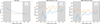 |
Fig. 1 Airmass and S/N plot over orbital phases. The gray area represents the out-of-transit phases. Due to better observational conditions (humidity and airmass), the S/N is higher for the second transit. |
2 Observations and data reduction
We observed two transits of the UHJ TOI-1518 b with MAROON-X, a high-resolution (Rλ ∼ 85 000) optical (spectral coverage between 490 and 920 nm) spectrograph at the 8.1-m Gemini-North observatory in Hawaii. Recent observations showed the capacity of MAROON-X to characterize UHJs by detecting ions and volatile and refractory elements. It has also allowed the description of the time variation of the atmospheric signal during transit (also known as the “trail”) (Pelletier et al. 2023; Prinoth et al. 2023) and even to study some strong lines such as Ca+ triplet (Prinoth et al. 2024). The observations were taken on 13 August 2022 and 10 October 2023 (program ID GN-2022B-Q-128 and GN-2023B-Q-127, PI: Parmentier). A summary of the observations is given in Table 1.
MAROON-X is divided into two detectors, one “blue” covering wavelengths ranging from 490 to 678 nm and one “red” covering wavelengths ranging from 640 to 920 nm. To ensure complete coverage of transit events, the observations include 30 min baseline measurements both pre- and post-transit. The exposure time for the red detector was slightly lower than for the blue arm (220s vs. 260s) during the first observation. For the second observation, the exposure time for both detectors was set up to 220 sec. Each order of the red detector comprises 4036 pixels, while the blue one has only 3954 pixels. There are 28 spectral orders for the red detector and 33 for the blue one. Fig. 1 presents the signal-to-noise ratio (S/N) and the airmass as a function of the observation frames for both transits. For both nights, the S/N was was always above 110, with a slightly better S/N for the second night (155 min and 210 max). During the second night, the blue arm seemed to perform less well than the red arm because the blue arm’s exposure time was higher during the first transit. Conditions of the second transit (average humidity =7% and lower airmass) were better, and so both arms still have better S/Ns than during the first transit (average humidity = 24%).
The MAROON-X data were reduced using the standard pipeline (Seifahrt et al. 2020) in one-dimensional wavelength-calibrated spectra and order by order for each time series exposure. The outputs are given as Norders × Nframes × Npixels, with Norders the number of spectral orders. In total, 40 frames were observed during both transits. The redder order of the blue detector (between 668 and 678 nm) was removed because the S/N is too low (<35).
One main limitation with high-resolution transmission spectroscopy from ground-based observations is the Earth’s atmosphere and stellar signals. Planetary signals are much fainter, but change over time because of the rapid Doppler acceleration, inducing shifts of many tens of km s−1 to the planet spectrum over the transit duration. The telluric lines, however, stay constant, and the positions of the stellar lines vary only by the order of 100 m s−1. This allows us to distinguish the planetary signal from the other two. We applied different reduction steps to the data following the sequence described by Pelletier et al. (2023) and summarized below:
All observed spectra are aligned in the stellar rest frame to remove the Earth’s barycentric motion and TOI-1518’s reflex motion. This is necessary to subtract the stellar signal from the data.
Each spectrum is set to the same continuum level to remove blaze and throughput variations.
The in-transit data are divided by a master stellar spectrum made with the averaged out-of-transit data.
A principal-component-analysis (PCA) approach removes the telluric signal and residuals from the stellar correction. For most species, we removed the first three principal components and verified that this was not significantly affecting our signal (see Fig. B.7). This is not the case for the Ca+ lines, which dominate the observed spectrum and are thus too affected by the PCA. For these, we decided to not use any PCA correction.
In Fig. 2, we show two orders of MAROON-X red detectors before (top) and after (bottom) the division by the master-out stellar spectrum. The strong stellar Ca+ lines are efficiently removed, leaving the planetary lines and the Doppler shadow effect apparent (see Sect. 3.4). In this wavelength range, the planetary Ca+ lines are clearly visible, even without PCA corrections.
Overview of TOI-1518 b observations during the two transits from program IDs GN-2022B-Q-128 and GN-2023B-Q-127; PI: Parmentier.
 |
Fig. 2 Correction of stellar and telluric signals. Top panel: raw data of two orders of MAROON-X red detector between 845 and 867 nm. Three strong stellar lines corresponding to the Ca+ triplet are observed around 849, 854, and 866 nm. Bottom panel: residuals obtained after correction with out-of-transit data. The dark signal here is the planetary Ca+ absorption lines, while the yellow signal is the Doppler shadow discussed in Sect. 3.4 that is caused by the Rossiter-McLaughlin effect. |
3 Cross-correlation analysis
3.1 TOI-1518 system
The ultra-hot Jupiter TOI-1518 b was discovered by Cabot et al. (2021). It is a 1.875 RJup planet with an equilibrium temperature for zero albedo of 2546 K. The planet is misaligned, with an impact parameter of 0.9 (see Table 2), meaning that it does not cross the zero-velocity plane of the star. The planet is precessing and the impact parameter has been shown to vary through time (Watanabe et al. 2024). Between our observations, a change of 0.03 was expected, which is too small to affect our observations (from b = 0.91497 in 2019 to b = 0.8797 in 2022). The geometry of the system is presented in Fig. B.1.
The planet orbits a 7300 K F-type star, which is fast rotating. The fast rotation rate from the star impeded Cabot et al. (2021) from detecting the radial velocity motion due to the orbit of the planet. As such, Cabot et al. (2021) were only able to put an upper limit to the planetary mass. In Appendix A, we also report the first significant detection of TOI-1518 b in radial velocity, using the SOPHIE spectrograph. This allows us to validate the planetary nature of the transits and to better characterize the system’s parameters, in particular the planetary mass and the semi-major axis. SOPHIE measurements allowed us to pin-down the mass of TOI-1518 b to 1.83 ± 0.47 MJup (see Appendix A for details). Additionally, we analyzed 56 transits of TOI-1518 b captured by TESS, compared to only 24 analyzed in Cabot et al. (2021). This increased dataset has enabled us to refine the planetary ephemerides, including the semi-major axis. The improved parameters lead to a planetary semi-amplitude velocity of Kp=207.32±4.51, which is 10 km/s lower (1.5 sigma lower) than in Cabot et al. (2021).
TOI-1518 stellar and planetary parameters from Cabot et al. (2021).
3.2 Template spectra for cross-correlation
The cross-correlation method is needed to detect the faint planetary lines in the residuals obtained after PCA. We cannot detect most of them directly, except for a few individual lines (such as Ca+). Fortunately, atoms and molecules have many spectral lines, and a cross-correlation with a template boosts the signal, allowing a precise detection of the planetary spectrum. A template is needed to combine these lines. We generated synthetic spectra specific to TOI-1518 b using the parameters from Table 2 and PetitRadtrans (Mollière et al. 2019), assuming a temperature of 2500 K, with chemical abundances determined by equilibrium chemistry and calculated with FastChem (Stock et al. 2022). We produced spectra for individual molecules at a resolution of Rλ = 250 000 over the 400 to 1000 nm wavelength range. These single-species spectra, to be used as cross-correlation templates, use collision-induced absorption (CIA) cross-sections of H2-H2 and H2-He as continuum. We then interpolated the spectra onto the MAROON-X wavelength grid and convolved them to match the instrumental resolution. The spectra were also convolved with the planetary rotation kernel. These spectra are shown in Fig. 3. The species selected in this study are based on those previously detected in recent MAROON-X publications (Prinoth et al. 2023; Pelletier et al. 2023).
Line lists from the Kurucz database were used for all atoms and ions (Kurucz 2017). For TiO, we used the TOTO line list (McKemmish et al. 2019). For VO, both the HyVO line list (Bowesman et al. 2024) and the VOmyt line list (McKemmish et al. 2016) outputs were compared in Sects. 3.3 and 3.5.
Alkaline metals and ions show individual strong lines, while other metals show line forests. Most of the signals except for the Ca+ triplet are stronger in the blue part of the spectrum, which corresponds to the blue detector of MAROON-X. We decided to analyze each detector individually as if it were two different transits and then to sum every Kp−Vres map or cross-correlation-function (CCF) map.
3.3 Species detected in the Kp−Vres maps
We converted the cross-correlation maps into velocity-velocity maps (Kp−Vres diagrams) by shifting them to the expected rest frame of the planet (Kp = 207.32 ± 4.51 km s−1, Vsys = −13.94 ± 0.17 km s−1), assuming values of projected orbital velocity between 0 and 400 km s−1 in steps of 1 km s−1. Fig. 4 shows 14 clear detections obtained via cross-correlating the signal with single-species templates. The white cross in each plot is the position of the expected signal from the planet if the planetary atmosphere is considered static and the planet has a circular orbit. The expected Kp is calculated as follows:
 (1)
(1)
with  , where P is the period, am is the semi-major axis of TOI-1518 b, and i is the inclination of the system. All these parameters are given in Table 2. To compute our Kp − Vres plots, we selected a range of orbital velocity (Kp) from 0 to 400 km s−1 and a range of rest-frame velocity (Vres) from −150 to 150 km s−1 with steps of 1 km s−1 for each. We then integrated each point of the CCF maps previously obtained (see Fig. 4) following the slope determined by the orbital velocity at the rest-frame position determined by Vres. The noise level is calculated in a region far from the central peak at Vres ≥ 75 km s−1, where no signal of the planet or Rossiter-McLaughlin (RM) residuals is expected. Fourteen species are detected with an S/N ≥ 4. The parameters of the best Gaussian fits of the Kp−Vres maps are presented in Table 3.
The Kp − Vres of other species of interested detected in other UHJs are presented in the appendix (see Fig. B.2). These ones show positive correlation near the expected orbital position and may warrant follow-up observations. On average, most species have a blueshifted signal compared to the expected velocity (Vres = ΔVsys ≈ −2.9 km s−1). The orbital velocity is also lower than expected (ΔKp ≈ −20.5 km s−1).
3.4 Trails of the signal in CCF maps
Figure 5 presents the time-variation of the CCF calculated with an Fe template and shifted into the planetary rest frame. The dashed yellow line on the right highlights the expected position of the planet if the atmosphere is static and homogeneous. As the planet is misaligned, the Doppler shadow effect (already observed in Cont et al. 2021) only affects the planetary signal at the beginning of the transit, and we thus decided to not mask it or remove it.
The Fe track shown in Fig. 5 is slightly shifted from the theoretical planetary velocity computed with the orbital parameters of Table 2. Previous high-resolution observations have demonstrated the ability to resolve time variations of this atmospheric track (Ehrenreich et al. 2020; Borsa et al. 2021). We thus investigated this with our data. We binned the CCF similarly to Wardenier et al. (2024) to increase the planetary signal. We divided the 25 in-transit frames observed in both datasets into nine bins. We used scipy.optimize. curve_fit to fit a Gaussian to each bin within ± 10 km/s in the planetary rest frame. This gave better results than performing the fit across a broader range of velocities. The results are shown in Fig. 6. The velocity center of the atmospheric track changes with time (Fig. 6, left panel), becoming more blueshifted from around +1 km s−1 to around −8 km s−1. This is similar to what happens in the case of other UHJs like WASP-76b and WASP-121b (Ehrenreich et al. 2020; Borsa et al. 2021). The signal’s amplitude reaches its peak during mid-transit, rather than at the beginning or the end.
We further detected the time-varying trace of the CCF for six different species: Fe, Fe+, Ca, Ca+, Na, and Mg (Fig. 7). All species show a qualitatively similar behavior to the Fe trace, with a blueshift over time.
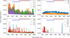 |
Fig. 3 Synthetic transmission spectra computed with PetitRadtrans and FastChem used as templates for the cross-correlation analysis. They are computed for TOI-1518 b parameters, assuming a temperature of 2500 K. The wavelength coverage of MAROON-X used in this study is represented with blue (blue detector, 490–670 nm) and red (red detector, 640–920 nm) lines. Ions and alkalines have few very strong lines, while other metals are composed of line forests. Molecules also have forests of spectral lines grouped in distinct absorption bands. Except for the Ca+ lines, the other metals present strong signals in the range of the blue detector of MAROON-X, where few telluric lines are present. At 2500 K, the Fe+ and Cr+ lines are smaller than the others and are not visible in this plot. |
3.5 Discussion
The equilibrium temperature of TOI-1518 b (2492 K, Cabot et al. 2021) is lower than that of WASP-189 b (2641 K, Anderson et al. 2018) and higher than that of WASP-76 b (2228 K, Ehrenreich et al. 2020), two recently UHJs observed with MAROON-X (Pelletier et al. 2023; Prinoth et al. 2023). Thus, each species observed in both planets is expected to be present in TOI-1518 b. The detection of Fe, Mn, Cr, V, Mg, Ca, and Na is thus consistent with previous observations. The non-detection of K is due to the overlap of the telluric water lines with the Doppler-shifted K lines. This is the consequence of an unfortunate systemic velocity and barycentric velocity during these two observations. The detection of Ti in TOI-1518 b, while it was not present on the cooler WASP-76 b but present on the hotter WASP-189 b, might be a sign that there is a trend of Ti abundance with temperature, possibly linked to the formation of TiO or to the nightside condensation of Ti. Whereas TiO would be expected in TOI-1518 b, we are not able to find it.
The detection of VO was made with a significance level of 4.9 sigma using the HyVO line list that was newly released this year (Bowesman et al. 2024). VO is notoriously difficult to detect in exoplanet atmospheres; however, Pelletier et al. (2023) demonstrates the feasibility of such detections when employing a more accurate line list. For WASP-76b, the VOmyt line list was useful for the detection of VO. Fig. 8 illustrates that this line list was unsuccessful in retrieving VO signals in the observations of TOI-1518 b. This discrepancy can be attributed to a stronger VO signal in WASP-76b, along with the use of three transit observations compared to only two for TOI-1518 b. In this study, we demonstrate the superior capability of the HyVO line list, which successfully detected VO (see Fig. 8). The detected signal is blueshifted by as much as −12.11 ± 0.22 km/s (see Table 3), which is significantly higher than the maximum blueshift observed for other species in TOI-1518 b (recorded at −5.16 ± 0.57 km/s). Currently, it remains uncertain whether this difference is due to a shift in the line list itself or a physical shift in the atmosphere, potentially stemming from the varying localization of VO compared to metals and ions in the atmosphere of TOI-1518 b. The presence of strong optical absorbers such as VO and TiO in the atmosphere of UHJs is crucial for thermal inversion phenomena (Fortney et al. 2008). This finding underscores the significance of utilizing more accurate line lists for the detection of these molecules, especially in cases where the signals may be weaker than those observed in WASP-76b. Further studies employing this new line list could reveal the presence of VO in targets where it was previously undetectable, as highlighted in Borsa et al. (2021).
Detecting Fe and Fe+, Ca and Ca+, Ti and Ti+, and potentially V and VO raises questions. For example, Fe+ is expected more in the hotter dayside atmosphere, whereas Fe should be more present on the cooler limbs and nightside. However, the tracks of Fe and Fe+ seen in Fig. 7 show a similar blueshifting trend, meaning that they are likely probing similar atmospheric regions. Additionally, the Fe trail of TOI-1518 b observed in Figs. 5 and 6 follows a comparable trend to the ones previously observed in WASP-76 b (Ehrenreich et al. 2020), WASP-121 b (Borsa et al. 2021), and WASP-189 b (Prinoth et al. 2023), with a signal becoming more blueshifted with the transit.
One of the main uncertainties of this work is the impact of the PCA step on the planetary signal. Fig. B.7 shows the Fe Kp−Vres map for three components removed on the left, and on the right it shows the maximum of the Kp−Vres map in the function of the number of PCA components removed for three different boxes where we measured the standard deviation of the map. The effect of PCA on high orbital velocity residuals is less than that on low velocity residuals, so calculating the standard deviation in the red box will underestimate the S/N. Conversely, the effect of PCA on low velocity residuals is much stronger, so the residuals will be smaller than those for high velocity, and the S/N will be overestimated. We then decided to calculate the standard deviation from the blue box, which mitigates this effect by taking the residuals at each velocity – but still far from the RM residuals or planetary signals – to avoid misinterpreting the standard deviation of the residual. The same method was used for each species observed.
Several Kp−Vres maps, such as Fe, Mg, Ca, or Cr, show a parasitic signal at Kp ≈ 90 km/s and Vres ≈ −60 km/s. This signal is a residual of the Rossiter-McLaughlin effect observed in the CCF map in Fig. 5. The Rossiter-McLaughlin effect presents an anticorrelation signal at negative Kp. Therefore, it is not shown here, but the residual positive correlation visible in yellow around the anticorrelation signal in the CCF map is the parasite signal observed in the Kp − Vres diagram mentioned previously. Possible biases due to the Rossiter Mc-Laughlin effect are present at a phase below −5 degrees and are represented in gray on the trail map of Fig. 7. The positive correlation at phases above 5 degrees is far from the planetary signal 5 (<−50 km/s). For the case of Mg, a signal is also visible at expected Kp, but Vres = 100 km s−1. This is due to a strong Fe+ line in the Mg triplet. This is also visible in the CCF maps of both species, where the residual signal of the other can be observed as highlighted in Fig. B.3.
Figure B.5 highlights some limitations of the Gaussian profiles used to parameterize the Fe trail of TOI-1518 b, as most one-dimensional CCFs do not follow a simple Gaussian profile. Then we decided to center the fit Gaussian profile on the maximum of the 1D-CCF, even if this resulted in a misestimation of the FWHM and probably of the error bars of the measured Vres. Another uncertainty might be due to the PCA applied to the data. Fig. B.4 presents the Fe trail of TOI-1518 b with different numbers of principal components removed. The square root of the variance of the Doppler shifts across all numbers of removed components, σ PCA was added to the uncertainty quoted in the covariance matrix of the Gaussian fit obtained from scipy.optimize.curve_fit. The PCA does not change the transit trend even when many components are removed for all species except Ca+ (Fig. B.6). The PCA is essential for detecting faint species. To maintain consistency, we removed the same number of components (three) from all species, even for those where it might not have been necessary. The only exception is Ca+, as the PCA significantly impacts the signal, even when fewer components are removed, due to its very high signal strength. Therefore, we decided not to apply PCA to Ca+ in order to achieve a more robust analysis of its trail.
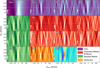 |
Fig. 4 Entire Kp − Vres diagram for detected species in TOI-1518 b dataset. The white cross indicates the expected location of the planetary signal, which assumes a static atmosphere. Deviations from the white cross could be the significance of wind, circulations, or chemical asymmetries on TOI-1518 b. A clear signal is observed with a white blob – sometimes shifted – near the white cross in each diagram. The signal observed at Kp around 100 km s−1 and Vres around −60 km s−1 in some diagrams is due to the Doppler shadow and is not of planetary origin. We note that the Ca+ Kp − Vres map was computed without the use of PCA (see discussion). |
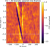 |
Fig. 5 Cross-correlation maps for Fe in planetary rest frame. The dashed yellow lines of the left panel represent the trace of the planetary signal at the expected Kp − Vres. The dashed yellow line of the right panel represents the position of the planetary signal if the atmosphere is static. The dashed white line represents the ingress part if the transit where we cannot distinguish the planetary signal (positive signal near 0 km/s) and the Doppler shadow (negative and positive signal diagonally from −130 to 0 km/s). |
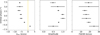 |
Fig. 6 Position (left panel), amplitude (central panel), and width (right panel) of the in-transit atmospheric CCFs’ Gaussian fit as a function of the orbital phase. The dashed yellow line of the left panel represents the expected position of the atmospheric track in the case of a static and homogeneous atmosphere. |
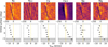 |
Fig. 7 Upper panel: CCF map of TOI-1518 b for six different species. Lower panel: position of maximum Gaussian fit of the CCF maps of the upper panel. The dashed yellow line of the left panel represents the expected position of the atmospheric track in the case of a static and homogeneous atmosphere. |
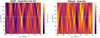 |
Fig. 8 Kp − Vres map of VO in TOI-1518 b with two different line lists. Left panel: CCF made with HyVO line list (Bowesman et al. 2024). Right panel: same, but with VOmyt line list (McKemmish et al. 2016). |
4 Comparison with global circulation models
To understand the physics behind the six time-resolved absorption trails we observed, we now compare our data with a suite of GCMs.
4.1 Model description
We considered five SPARC/MITgcm models of TOI 1518 b. Three are presented in Fig. 9. The SPARC/MITgcm was initially introduced by Showman et al. (2009). It has been widely used to study the atmospheric physics and chemistry of (ultra)hot Jupiters (Fortney et al. 2010; Showman et al. 2013; Kataria et al. 2013; Parmentier et al. 2018). Our cloud-free models of TOI-1518 b are based on work by Tan et al. (2024). As in previous works (Showman et al. 2013; Komacek & Showman 2016; Parmentier & Crossfield 2018), we parameterized several source of dissipation (including turbulent mixing (Li & Goodman 2010), shocks (Heng 2012), hydrodynamic instabilities (Fromang et al. 2016), and magnetic drag (Perna et al. 2010; Beltz et al. 2022)) through a Newtonian relaxation term in velocity applied to the momentum equation. The relaxation timescale, called the drag timescale hereafter, ranges from τdrag = 103s (strong drag) to τdrag = 106s (weak drag).
These GCMs account for heat transport due to H2 dissociation and recombination (e.g., Bell & Cowan 2018; Komacek & Tan 2018; Tan & Komacek 2019; Roth et al. 2021). H2 thermally dissociates on the dayside, after which point atomic hydrogen is advected to the nightside, where it recombines into H2 and releases latent heat. When the atmospheric circulation is predominantly eastward, most of this heat is pumped on the evening limb, resulting in a temperature asymmetry between the eastern and western regions of the atmosphere (first and second columns in Fig. 9). Drag restores energy to the atmosphere. Increasing drag strength (i.e., lowering τdrag) slows down winds in the atmosphere hindering this model’s heat transport. In strong-drag cases, the temperature structure becomes symmetric, resulting in similar chemical compositions in the morning and evening limbs (last column in Fig. 9). In the strong-drag model, there is only a day-to-night flow as the equatorial jet is suppressed (Showman et al. 2013). Table 4 summarizes some other important parameters of the two SPARC/MITgcm models. We refer the reader to Table 1 in Tan et al. (2024) for the full list of opacities considered in their radiative transfer (which include species such as TiO and Fe driving thermal inversion on the planet’s dayside). All models were run at a horizontal resolution of C32, corresponding to roughly 128 cells in longitude and 64 in latitude. Before computing phase-dependent spectra of the GCMs with gCMCRT, we binned the outputs down to 32 latitudes and 64 longitudes, as in Wardenier et al. (2021, 2023, 2024).
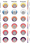 |
Fig. 9 Overview of three of five GCM models of TOI-1518 b considered in this work. The model in the first column is the drag-free model, while the second and last columns consider, respectively, weak (τdrag = 106s) and strong (τdrag = 103s) drag effects. Each panel shows the planet’s equatorial plane, with the relative size of the atmosphere inflated for visualization purposes. From top to bottom, the rows show the temperature structure; the line-of-sight velocities due to winds (at mid-transit); and the spatial distribution of Fe+, Fe, Ca+, and Ca, respectively. The white dashed contours in each plot represent isobars with pressures P = 101, 10−1, 10−3, 10−5 bar. |
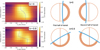 |
Fig. 10 Importance of impact parameter b with examples for b=0 on the top row and b =0.9 on the lower row. On the left, the CCF maps of the injected models within blue dashed lines and the Gaussian fit applied similarly to the data (Fig. 6). On the right, the illuminated part of the limb during the first and second half of the transit is represented in a vertical slice and shown to scale. |
4.2 Injection and cross-correlation maps
We computed phase-dependent transmission spectra of the five GCM models across the MAROON-X spectral range (between 490 and 920 nm) using gCMCRT (Lee et al. 2022). The calculations account for Doppler shifts due to planet rotation and winds. Section 2 of Wardenier et al. (2023) shows the radiative transfer and post-processing details. Therefore, we only briefly summarize the gCMCRT setup for TOI-1518 b analysis. Before feeding the GCM outputs into gCMCRT, we mapped the atmospheric structures onto a 3D grid with altitude (instead of pressure) as a vertical coordinate. We accounted for the fact that each atmospheric column has a different scale height set by local gravity, temperature, and mean molecular weight. For each of the five TOI-1518 b models, we simulated 25 spectra (equidistant in orbital phase) between phase angles ± 8 degrees, covering the in-transit part of our observations. At each orbital phase angle, gCMCRT simulated a transmission spectrum by randomly shooting photon packets at the part of the planet limb that is blocking the star and evaluating the optical depth encountered by each photon packet. Due to the geometry of TOI-1518 b (Fig. B.1), the part of the planet that is illuminated differs from the case of WASP-121 b, where the impact parameter is near zero (Fig. 10, Right Panel). In this calculation, the code accounts for Doppler shifts imparted on the opacities by the radial component of the local wind vector and planet rotation (Wardenier et al. 2021). The transit depth at a specific wavelength is calculated by averaging it over all photon packets. To accurately represent the shapes, depths, and shifts of the spectral lines, we used 105 photon packets per wavelength. Since we did not explicitly account for scattering, the direction of propagation for the photon packets remains constant throughout the calculation. The spectra were simulated at a native resolution of R = 300 000 and then convolved down to the instrument resolution of Rλ = 85 000, which differs from Wardenier et al. (2023, 2024). We included the same set of continuum opacities and line species for the radiative transfer as in Wardenier et al. (2023). To properly compare the GCM spectra with the data, we need to inject the GCMs into the data and perform PCA, similarly to what we did for the data. The different steps are listed below:
Inject the spectra at each orbital phase into the three components that were removed during the data reduction process, using the Kp velocity value from Eq. (1);
Perform PCA on the data + GCM removing three components, the same number of components as for the data in the case of Fe;
Subtract the post-PCA data from the combined data+GCM to isolate the GCM signal post-PCA and remove the noise;
Do the cross-correlation with the same Fe template and methods used for Sect. 3.2.
The resulting CCFs for the case of the drag model are shown in Fig. 10. The difference between the two models at different impact parameters b is also represented with the case of b = 0 on the upper row and b = 0.9 on the lower row.
We then interpolated the cross-correlation results over the same phase grid as for the observations of the two transits. We then performed the same analysis using the fit with a Gaussian profile, which allowed us to extract the position, amplitude, and FWHM of the model’s signal. Figs. 11 and 12 show the CCF signals of Fe and Fe+ that we obtain for each of the models, with the real data plotted on top.
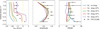 |
Fig. 11 Same as Fig. 6, but with results of Gaussian fit for different models from “no drag effect” to “strong drag effect”. In the central panel, the illuminated fraction of the planetary limb as a function of the orbital phase is represented by a dashed yellow line. |
4.3 Discussion
Figure 11 (left panel) shows the Fe trails of the five GCM simulations, along with the Doppler shifts of Fe measured in Sect. 3.2. All models show a signal that is blueshifting with time. This behavior was previously observed by Ehrenreich et al. (2020); Borsa et al. (2021) and discussed in many papers (Wardenier et al. 2021, 2023; Savel et al. 2022; Beltz et al. 2022, 2023). Because the planet rotates during the transit, the start of the transit probes the dayside of the leading limb and the nightside of the trailing limb. It is thus dominated by the hotter leading limb. The planet rotation redshifts the leading limb by ≈3.5 km/s, which is compensated by the blueshift of the day-to-night winds. In the second part of the transit, the opposite happens and the signal is dominated by the trailing limb, which is blueshifted by rotation. The change from being dominated by the leading and the trailing limbs during transit is responsible for the blueshifting of the signal with time.
In the case of TOI-1518 b’s atmosphere, the high impact parameter reinforces this blueshift. Indeed, as shown in Fig. 10, because the planet is close to grazing, we almost never probe the full atmospheric limb. The signal from the first half of the transit is therefore entirely due to the leading limb, with only a very small contribution to the trailing limb, and the opposite is true for the second part of the transit. As a consequence, we find that a given planet is expected to have a stronger blueshift with time when observed with a high impact parameter than with a low impact parameter.
Furthermore, the global shift of the planetary trace is linked to the day-to-night winds that blueshift both leading and trailing hemisphere signals. These day-to-night winds are strongly affected by drag. As shown in Fig. 11, models without drag produce an Fe signal that is too blueshifted compared to the observations. Overall, the planetary signal stands between the stronger drag models (τdrag = 104 and 103 s). When looking at the amplitude and at the FWHM of the signal, however, we see that the τdrag = 104 s model is favored, because the τdrag = 103 s provides a signal that is too small and not wide enough compared to data.
If we now look at the Fe+ trace (Fig. 12), we see that the τdrag = 104 s overestimates the blueshift, whereas the τdrag = 103 s (purple) is a much better match. For Fe+, the amplitude of the model is unaffected by the drag, and the FHWM errorbars are too large to differentiate between the two strong-drag models. The apparent contradiction between the Fe trace favoring the τdrag = 104 s model and the Fe+ trace favoring the stronger τdrag = 103 s drag model could be an indication of the presence of ohmic drag in the atmosphere. Indeed, as shown by Beltz et al. (2022), ohmic drag strength strongly depends on planetary location because it is stronger in the hotter dayside and at lower pressures. Because the Fe/Fe+ equilibrium is temperature-dependent, the Fe+ signal naturally probes more into the hotter planetary dayside than the Fe signal, where the temperatures are hotter and magnetic drag effects are expected to be larger.
Figure 13 shows the trails for the six species of Fig. 7 with the signals of the stronger drag models. For Ca, Na, Mg, and Ca+, the signal straddles between both these GCMs, as in the case of Fe. We therefore confirm that the strong drag scenario is preferred by the signal of all the other species. A similar agreement with an intense drag model atmosphere was already observed in the case of WASP-121 b by Wardenier et al. (2024), pointing out that strong drag is common in ultra-hot-Jupiter atmospheres.
The trail of the Ca+ is significantly different from the ones of the other species, as it starts strongly redshifted. This is clearly not captured by the model. We calculated the contribution functions of our model and find that the CCF of most species (including Ca, Fe, and Fe+) probes the 10−3 and 10−5 bar layers, whereas the Ca+ probes layers up to 10−8. We directly fit the resolved individual Ca+ lines using a method similar to that of Prinoth et al. (2024) and found a transit depth corresponding to an effective radius of 1.97 ± 0.04 Rp. This value is similar to the planetary Roche radius (RRoches ≃ 1.96 Rp at Lagrange point 1 following Gu et al. 2003). As a consequence, we believe that the Ca+ lines likely probe the outflow of the planet. This region shows a different atmospheric flow than the deeper regions, with an important contribution from planet-star interactions, which is not modeled in our GCM. Our results for Ca+ are similar to the recent observations of H-alpha for WASP-121b (Seidel et al. 2025).
The CCF of the GCM, presented in Fig. 10, exhibits a double-peak structure with one centered near 0 km/s and another around −7 km/s. This feature arises from the contribution of both atmospheric limbs. Fitting this complex signal with a simple Gaussian profile is inherently limiting, as a single-peaked function cannot accurately capture the asymmetric nature of the CCF. Parameters such as the FWHM and amplitude may be misrepresented, potentially leading to an incomplete interpretation of the atmospheric dynamics. Finally, for VO, the predictions from the GCMs do not match the observed signal observed in Fig. 8. The GCMs estimate a change in Kp of about ± 5 km/s and a Vres ranging from −6 to −13 km/s (decreasing with decreasing drag) when the signal observed in the data is at ΔKp around −33 km/s and Vres is at around −13 km/s.
 |
Fig. 13 Same as lower panel of Fig. 7, but with results of Gaussian fit for stronger drag models included. |
5 Retrieval analysis
After detecting the species shown in Sect. 3.2 thanks to cross-correlation analysis, the next step was to explore the abundances of these species in comparison to solar values. This comparison is possible due to the solar metallicity of the host star. One approach developed in Brogi & Line (2019) is to use a Bayesian atmospheric retrieval framework with high-resolution cross-correlation spectroscopy (HRCCS) that relies on the crosscorrelation between data and models for extracting the planetary spectral signal. This approach allows the characterization of many atmospheres of UHJs and puts constraints on abundances (Line et al. 2021; Kasper et al. 2021, 2023; Brogi et al. 2023).
5.1 CHIMERA code
Following the above method, we applied the cross-correlation-to-log-likelihood retrieval framework from Brogi & Line (2019) to derive the molecular volume-mixing ratios and the temperature layer we were probing. For the retrieval process, we used the CHIMERA “free-retrieval” (Line et al. 2013; Kreidberg et al. 2015) paradigm, which assumes constant-with-altitude gas-mixing ratios and uses a simple isothermal T-P profile, which is an adequate approximation to retrieve abundances with MAROON-X as shown by Pelletier et al. (2023). We used a similar setup to Line et al. (2021), but with a wavelength range and a choice of chemical species adapted to the MAROON-X bandpass. Additionally, we used a native resolution for the radiative transfer of 500.000, which was downgraded to the MAROON-X 85.000 resolution after instrumental and rotational broadening and orbital Doppler shift. The retrieval parameters specific to our analysis and their prior ranges are provided in Table 5. A more detailed description of the high-resolution GPU-based radiative-transfer method and log-likelihood implementation within pymultinest (Feroz et al. 2009; Buchner et al. 2014) is given in Line et al. (2021).
Parameters and corresponding priors used in retrieval analysis with CHIMERA for the study of TOI-1518 b.
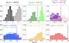 |
Fig. 14 Histograms of measured abundances of different elements in TOI-1518 b’s atmosphere. The proto-solar value of each element is represented by dashed lines (from Lodders 2019). |
5.2 Results of the retrieval analysis
We combined the blue- and red-arm MAROON-X data for our retrieval for both transits. We included most of the species detected in Sect. 3.2 + TiO and abundance proxies for the H- bound-free and free-free continua. However, some species detected in the cross-correlation analysis were not included in the retrieval framework due to a lack of opacity files in the right format, such as Ba+, Si, and Mn.
The mass prior was set using the SOPHIE observation results (see Table A.2) as a free parameter that follows a Gaussian distribution with Mp = 1.83 MJup ± 0.47. For this analysis, we considered the two detectors independently, as we did for the CCF, and we added the likelihood from the red and the blue detector analyses and then from both transits. For the retrieval analysis, we performed PCA on the data and the injected models, using the same number of components as in the CCF analysis. As shown before, the PCA does not strongly affect the planetary lines, apart from the ones of the Ca+. However, because the retrieval considers all species at the same time, we cannot have different PCA numbers per species. The results of the measured abundances are summarized in Fig. 14, and the whole corner plot is given in the appendix (Fig. D.2).
5.3 Discussion of the retrieval analysis
The Kp and Vres distribution of the retrieval analysis (Fig. D.2) are consistent with the Fe signal detected in Sect. 3.2. The measured Vres( km/s) and Kp(
 km/s) also agree with the detection of Cabot et al. (2021) (
 km/s. and
  km/s). With a Δ Kp of approximately −25 km/s compared to the Kp derived from the SOPHIE data, and a Vres around −3 km/s, the retrieval also captures the blueshift of the signal as a function of the planet’s orbital phase, as detailed in Sect. 4. We observed that the velocity parameters obtained are influenced predominantly by the strongest absorber, particularly Fe.
Our model retrieves an Fe abundance of  . This corresponds to 0.07 to 1.62 solar enrichment in Fe. This remains consistent with a solar (and then stellar) metallicity. We checked that the Fe abundance was robust to different assumptions in the retrieval, and that it was not changing when different other species were added.
The retrieval results for the other chemical species are more surprising and highlight the difficulty of atmospheric retrievals for transit spectroscopy at high spectral resolution. First, the ionized species, such as Fe+ and Ca+ have retrieved abundances that are much higher than solar. These high abundances, up to  , are unlikely in a gas giant atmosphere. Instead, we believe that these could stem from a lack of flexibility in the forward model. Indeed, ionized species are more likely to probe different parts of the atmosphere (both vertically and longitudinally) than neutral species, because the spatial repartition of neutral and ionized forms of the same species is anticorrelated. This can lead to signals at different temperatures and Kp and Vres (e.g. Table 3). However, given that the temperature, Kp, and Vres for all species are determined by the neutral Fe lines, which represent the strongest signal, the abundances of the other species are likely biased to compensate for the Kp/Vres offset. For lines with a strong Kp/Vsys shift and small opacities, such as Cr, V, Ti or VO, the retrieval leads only to upper limits, which are all consistent with a solar enrichment.
For the Ca and Mg lines, the retrieval provides a detection with an abundance of  and
and  , corresponding to 0.0002 to 0.034 times the solar abundance for Ca and 0.0004 to 0.339 times solar for Mg. The retrieved value for Ca is significantly lower than that of Fe, and it is, for now, unclear whether this is due to a physical effect (e.g., most Ca being into Ca+) or a bias in the retrieval. Finally, our results for VO deserve a special mention.
Despite using the latest VO line list, the multi-species retrieval did not successfully detect VO. To explore this issue further, we conducted a single-species retrieval focused solely on VO (see Fig. D.1). This approach resulted in a detection with a temperature around 2700 K, compared to 3500 K in the multi-species retrieval, along with a different Kp − Vres distribution (Fig. 15). The measured value of VO in such a framework is  , corresponding to an enrichment of 1.10 to 45708.81 times solar. The discrepancy in the Kp − Vres distribution resembles the patterns observed in the Kp − Vres map (see Table 4). This difference could be attributed to either dynamical factors – if VO probes specific regions of the atmosphere – or inaccuracies in the positioning of the lines within the VO line list. This situation underscores the limitations of the current framework in accurately deriving abundance for species that are settled in a different Kp − Vres distribution.
Further observations with bluer or redder instruments to detect molecules or ionized species are needed to determine why such elements are subsolar. Moreover, using a non-isothermal profile instead would have a dual effect on the spectrum. First, it would produce a similar effect to an abundance gradient by stretching the spectral lines. Second, it would enhance the abundance gradient in the case of chemical equilibrium, further impacting the observed spectral features. Incorporating more realistic temperature and abundance gradients in future retrieval analyses will be essential to better constrain the abundances of ionized species.
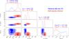 |
Fig. 15 Likelihood distributions for temperature, Kp, Vres, and log 10 VO derived from the multi-species retrieval (in red) and from retrieval with only VO inside (in blue). |
6 Conclusions
This study presents an in-depth analysis of TOI-1518 b, an ultrahot Jupiter. We used transit observations from MAROON-X on Gemini-N to explore its atmospheric dynamics and chemical composition. Our findings offer new insights into the unique characteristics of this extreme exoplanet. Using the SOPHIE spectrograph, we also report the first significant detection of TOI-1518 b in radial velocity. This allows us to better characterize the system, and in particular to measure the planetary mass MP = 1.83 ± 0.47 MJup.
Our cross-correlation analysis focused on detecting atomic and molecular species within the atmosphere. We report the detection of 14 different species. High-resolution spectroscopy allowed us to identify ionized and neutral species with ionized metals such as Fe+, Ca+, and Ti+. The detection of these ionized species, as opposed to their neutral counterparts, underscores the extreme temperatures of TOI-1518 b’s atmosphere, where thermal ionization is significant. Additionally, we report the detection of VO, a critical absorber that has implications for thermal inversions in UHJs. The presence of VO adds a crucial piece to the puzzle of understanding the thermal structure and chemical processes in such extreme environments. This was possible thanks to the newer HyVO line list that should be used in other studies were detection of VO failed with previous line lists.
We investigated the atmospheric wind dynamics by analyzing the blueshift of multiple species in the observed spectra as a function of the planet’s orbital phase. The blueshift of Fe is consistent with previous observations of other UHJs. By combining the signal from different species, particularly Fe+ and Fe, and comparing them with GCMs, we conclude that a strong drag is needed (τdrag = 103−−104 s) to explain the data. Fe+ seems to need more substantial drag compared to Fe, which can be due to the increased ohmic drag on the planetary dayside. Finally, we find that the trail of Ca+ is very different from the other species, which is likely due to Ca+ probing the escaping atmosphere above the Roche lobe while all other species probe deeper atmospheric pressures.
The retrieval analysis provided constraints to the abundance of various chemical species in the atmosphere. We report an abundance of Fe of  , which is consistent with a solar enrichment. The retrieval being driven mainly by Fe, we believe that the Fe abundances are robust. However, most other species are detected at a different Kp/Vres, which our retrieval framework does not consider. As a consequence, we believe that the retrieved abundance for the other species are strongly biased. We studied this bias in more detail for the specific case of VO, for which our main retrieval does not find a signal, but where a retrieval without Fe lead to a detection at a different temperature, Kp, Vres, and an abundance of 1.10 to 45708.81 times solar.
Overall, our study demonstrates the power of combining high-resolution spectroscopy with advanced modeling techniques to probe the atmospheres of UHJs. They shed light on the specific properties of TOI-1518 b and contribute to the broader understanding of atmospheric dynamics and chemistry in these extreme exoplanets. Future studies should continue to refine these models and expand observational efforts to explore the diversity and complexity of UHJ atmospheres.
Acknowledgements
This work was partially funded by the French National Research Agency (ANR) project EXOWINDS (ANR-23-CE31-0001-01). This work was supported by the French government through the France 2030 investment plan managed by the National Research Agency (ANR), as part of the Initiative of Excellence Université Côte d’Azur under reference number ANR-15-IDEX-01. The authors are grateful to the Université Côte d’Azur’s Center for High-Performance Computing (OPAL infrastructure) for providing resources and support. J.P.W. acknowledges support from the Trottier Family Foundation via the Trottier Postdoctoral Fellowship. M.R.L. and J.L.B. acknowledge support from NASA XRP grant 80NSSC19K0293 and NSF grant AST-2307177. J.L.B. acknowledges funding for the MAROON-X project from the David and Lucile Packard Foundation, the Heising-Simons Foundation, the Gordon and Betty Moore Foundation, the Gemini Observatory, the NSF (award number 2108465), and NASA (grant number 80NSSC22K0117). This work uses observations secured with the SOPHIE spectrograph at the 1.93-m telescope of Observatoire Haute-Provence, France, with the support of its staff. This work was supported by the “Programme National de Planétologie” (PNP) of CNRS/INSU, and CNES.
Appendix A Measurement of the planetary mass
Cabot et al. 2021 obtained a hint (less than 2σ significance) for a radial-velocity (RV) detection of TO-1518b using the FIES spectrograph. They reported an RV semi-amplitude of 152 ± 75 m/s, which they converted to a 2−σ upper limit of 281 m/s, corresponding to a planetary upper mass limit of 2.3 MJup.
With the goal to improve the constraint on the planetary mass, we observed TOI-1518 with the SOPHIE spectrograph at the 1.93-m telescope of the Observatoire de Haute-Provence, France. SOPHIE is a stabilized échelle spectrograph dedicated to high-precision RV measurements (Perruchot et al. 2008; Bouchy et al. 2009, 2013). We used its high-resolution mode (resolving power R = 75 000) and fast readout mode. We obtained exposures at 14 different epochs between December 2023 and January 2024. Exposure times ranged between 3.9 and 16.8 minutes depending on weather conditions, allowing signal-to-noise from 35.6 to 47.3 to be reached per pixel at 550 nm. The log of the observations is reported in Table A.1.
The RVs were extracted with the SOPHIE pipeline, as presented by Bouchy et al. (2009) and refined by Heidari et al. (2024). It derives cross correlation functions (CCF) from standard numerical masks corresponding to different spectral types. As expected from the known rapid rotation speed of the star, the derived CCFs were broad, with typical FWHM around 100 km/s. So to measure the RV, instead of fitting a Gaussian profile as it is standardly done for slow rotators, here we fitted the CCF with a profile constructed from the convolution of a Gaussian and a rotational profile following Gray (2022). This provided good fits of the CCFs. The Moonlight pollution, estimated using the second SOPHIE fiber aperture that is targeted on the sky, 2’ away from the first one pointing toward the star, was negligible.
The FWHM of the Gaussian is unknown, but is expected to be small by comparison to the FWHM of the rotational profile. We attempted free and fixed values for that Gaussian FWHM, which did not significantly modify our results. We finally fixed the FWHM of the Gaussian profile to 7 km/s on each exposure, which is a common value for such kind of stars. The FWHM of the rotational profile was free to vary among exposures, and we obtained values corresponding to v sin i* = 78.9 km/s, with a dispersion of ± 1.1 km/s. This is in good agreement with the values v sin i* = 85 ± 6 km/s reported by Cabot et al. 2021. The measured RVs (see Table A.1) are derived from the fitted center of the Gaussian and rotational profiles, constrained to be identical for a given epoch.
We phase-folded those SOPHIE’s RVs using the 1.9-d period derived from the transits observed by TESS. This provided a significant RV semi-amplitude  m/s, in phase with the transit epoch measured with TESS. This agrees with the upper limit reported by Cabot et al. (2021). So we concluded our SOPHIE data allow the planet TOI-1518 b to be significantly detected, for the first time with RVs.
To refine the system parameters, we made a joined fit of the TESS transit light curves and the available RVs. Following Heidari et al. (2025), we fitted that dataset using the EXOFASTv2 package (Eastman et al. 2013; Eastman 2017; Eastman et al. 2019). Cabot et al. (2021) used TESS sectors 17 and 18 covering TOI-1518, observed in FFI mode so with a long-cadence 30−min sampling, in addition to five ground-based photometric follow up. Here, we used both those TESS sectors, as well as the three additional TESS sectors covering TOI-1518 now available, which have a short-cadence 2-min sampling (sectors 57, 58, and 77). So by comparison to Cabot et al. (2021), the number of TOI1518 b individual transits included in our fit increases from 24 to 56. And in addition to our new SOPHIE RVs, we also used the FIES RVs published by Cabot et al. (2021).
SOPHIE measurements of the planet-host star TOI-1518
Cabot et al. (2021) reported a negligible eccentricity ( ). We tested eccentric and circular orbits without detecting significant differences, and finally adopted here a circular orbit. According to Watanabe et al. (2024), the system shows a change in the impact parameter b of the planet as a function of time. Over the 4.5-yr span of the TESS observations we use, the expected effect is of the order of 0.05 on b. This is not taken into account here, and we report averaged values. This has no significant impact on the reported planetary mass.
Our fitted RVs and transit light curve are shown in Fig. A.1 and A.2, respectively. We finally measured an RV semi-amplitude  m/s, corresponding to a planetary mass 1.83 ± 0.47 MJup. The full results of our fit are reported in Table A.2. Our derived parameters agree with those presented by Cabot et al. 2021, with improved uncertainties for most of them.
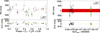 |
Fig. A.1 Radial velocities of TOI-1518 as a function of the planetary orbital phase (left) and time (right). SOPHIE (Table A.1) and FIES (Cabot et al. 2021) measurements are plotted in green and black, respectively, together with their 1−σ error bars. The fitted Keplerian orbit (Table A.2) is overplotted in red. The bottom panels show the residuals. |
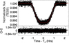 |
Fig. A.2 Phase-folded TESS transit light curve of TOI-1518. The fitted Keplerian orbit (Table A.2) is overplotted in red. The bottom panel shows the residuals. |
Median values and 68% confidence interval for the TOI-1518 system.
Appendix B Cross-correlation-function
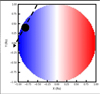 |
Fig. B.1 Qualitative geometry of the transit of TOI-1518 b. This planet is highly misaligned with the star (impact parameter =0.9). |
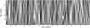 |
Fig. B.2 All Kp − Vres diagram for non-detected species in TOI-1518 b dataset. The white cross indicates the expected location of the planetary signal, which assumes a static atmosphere. The signal observed at Kp around 100 km s−1 and Vres around −60 km s−1 in some diagrams is an artifact due to the Doppler shadow. |
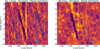 |
Fig. B.3 Trails of Fe+ and Mg with contamination from Mg in Fe+ trail and Fe+ in Mg trail due to the proximity of a strong Fe+ feature in the Mg triplet. |
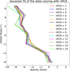 |
Fig. B.4 Measured Doppler shifts for Fe as a function of orbital phase angle. Different colors represent different numbers of components removed from the data. |
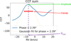 |
Fig. B.5 Example of the Gaussian fit applies to one binned CCF result. The blue line is the CCF binned for one orbital phase. In the yellow dashed line, the Gaussian fit performs where we infer the three parameters presented in Fig. 6 and Fig. 11. |
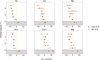 |
Fig. B.6 Same as lower panel of Fig. 7 but with the results of the Gaussian fit for the study with and without PCA. |
 |
Fig. B.7 Comparison of the S/N level obtained as function of number of PCA components with different boxes used for the calculation of the standard deviation of the Fe Kp − Vres map. |
Appendix C Global circulation models
Appendix D Retrieval analysis
 |
Fig. D.1 Corner plot of the single species retrieval with only VO |
 |
Fig. D.2 Corner plot of the full retrieval analysis |
References
- Anderson, D. R., Temple, L. Y., Nielsen, L. D., et al. 2018, arXiv e-prints [arXiv:1809.04897] [Google Scholar]
- Bell, T. J., & Cowan, N. B., 2018, ApJ, 857, L20 [Google Scholar]
- Beltz, H., Rauscher, E., Roman, M. T., & Guilliat, A., 2022, AJ, 163, 35 [NASA ADS] [CrossRef] [Google Scholar]
- Beltz, H., Rauscher, E., Kempton, E. M. R., Malsky, I., & Savel, A. B., 2023, AJ, 165, 257 [NASA ADS] [CrossRef] [Google Scholar]
- Borsa, F., Allart, R., Casasayas-Barris, N., et al. 2021, A&A, 645, A24 [EDP Sciences] [Google Scholar]
- Bouchy, F., Hébrard, G., Udry, S., et al. 2009, A&A, 505, 853 [NASA ADS] [CrossRef] [EDP Sciences] [Google Scholar]
- Bouchy, F., Díaz, R. F., Hébrard, G., et al. 2013, A&A, 549, A49 [NASA ADS] [CrossRef] [EDP Sciences] [Google Scholar]
- Bowesman, C. A., Qu, Q., McKemmish, L. K., Yurchenko, S. N., & Tennyson, J., 2024, MNRAS, 529, 1321 [NASA ADS] [CrossRef] [Google Scholar]
- Brogi, M., & Line, M. R., 2019, AJ, 157, 114 [Google Scholar]
- Brogi, M., Emeka-Okafor, V., Line, M. R., et al. 2023, AJ, 165, 91 [NASA ADS] [CrossRef] [Google Scholar]
- Buchner, J., Georgakakis, A., Nandra, K., et al. 2014, A&A, 564, A125 [NASA ADS] [CrossRef] [EDP Sciences] [Google Scholar]
- Cabot, S. H. C., Bello-Arufe, A., Mendonça, J. M., et al. 2021, AJ, 162, 218 [NASA ADS] [CrossRef] [Google Scholar]
- Chachan, Y., Knutson, H. A., Lothringer, J., & Blake, G. A., 2023, ApJ, 943, 112 [NASA ADS] [CrossRef] [Google Scholar]
- Charbonneau, D., Brown, T. M., Noyes, R. W., & Gilliland, R. L., 2002, ApJ, 568, 377 [Google Scholar]
- Chauvin, G., Lagrange, A. M., Zuckerman, B., et al. 2005, A&A, 438, L29 [NASA ADS] [CrossRef] [EDP Sciences] [Google Scholar]
- Cont, D., Yan, F., Reiners, A., et al. 2021, A&A, 651, A33 [NASA ADS] [CrossRef] [EDP Sciences] [Google Scholar]
- Coulombe, L.-P., Benneke, B., Challener, R., et al. 2023, Nature, 620, 292 [NASA ADS] [CrossRef] [Google Scholar]
- Eastman, J., 2017, EXOFASTv2: Generalized publication-quality exoplanet modeling code, Astrophysics Source Code Library [record ascl:1710.003] [Google Scholar]
- Eastman, J., Gaudi, B. S., & Agol, E., 2013, PASP, 125, 83 [Google Scholar]
- Eastman, J. D., Rodriguez, J. E., Agol, E., et al. 2019, arXiv e-prints [arXiv:1907.09480] [Google Scholar]
- Ehrenreich, D., Lovis, C., Allart, R., et al. 2020, Nature, 580, 597 [Google Scholar]
- Espinoza, N., Steinrueck, M. E., Kirk, J., et al. 2024, Nature, 632, 1017 [CrossRef] [Google Scholar]
- Feng, Y. K., Wright, J. T., Nelson, B., et al. 2015, ApJ, 800, 22 [Google Scholar]
- Feroz, F., Hobson, M. P., & Bridges, M., 2009, MNRAS, 398, 1601 [NASA ADS] [CrossRef] [Google Scholar]
- Fortney, J. J., Lodders, K., Marley, M. S., & Freedman, R. S., 2008, ApJ, 678, 1419 [CrossRef] [Google Scholar]
- Fortney, J. J., Shabram, M., Showman, A. P., et al. 2010, ApJ, 709, 1396 [NASA ADS] [CrossRef] [Google Scholar]
- Fromang, S., Leconte, J., & Heng, K., 2016, A&A, 591, A144 [NASA ADS] [CrossRef] [EDP Sciences] [Google Scholar]
- Gray, D. F., 2022, The observation and analysis of stellar photospheres (Cambridge: Cambridge University Press) [Google Scholar]
- Gu, P.-G., Lin, D. N. C., & Bodenheimer, P. H. 2003, ApJ, 588, 509 [NASA ADS] [CrossRef] [Google Scholar]
- Heidari, N., Boisse, I., Hara, N. C., et al. 2024, A&A, 681, A55 [NASA ADS] [CrossRef] [EDP Sciences] [Google Scholar]
- Heidari, N., Hébrard, G., Martioli, E., et al. 2025, A&A, 694, A36 [NASA ADS] [CrossRef] [EDP Sciences] [Google Scholar]
- Heng, K., 2012, ApJ, 761, L1 [NASA ADS] [CrossRef] [Google Scholar]
- Kasper, D., Bean, J. L., Line, M. R., et al. 2021, ApJ, 921, L18 [CrossRef] [Google Scholar]
- Kasper, D., Bean, J. L., Line, M. R., et al. 2023, AJ, 165, 7 [NASA ADS] [CrossRef] [Google Scholar]
- Kataria, T., Showman, A. P., Lewis, N. K., et al. 2013, ApJ, 767, 76 [NASA ADS] [CrossRef] [Google Scholar]
- Kesseli, A. Y., Snellen, I. A. G., Casasayas-Barris, N., Mollière, P., & SánchezLópez, A., 2022, AJ, 163, 107 [NASA ADS] [CrossRef] [Google Scholar]
- Komacek, T. D., & Showman, A. P., 2016, ApJ, 821, 16 [CrossRef] [Google Scholar]
- Komacek, T. D., & Tan, X., 2018, RNAAS, 2, 36 [NASA ADS] [Google Scholar]
- Kreidberg, L., Line, M. R., Bean, J. L., et al. 2015, ApJ, 814, 66 [NASA ADS] [CrossRef] [Google Scholar]
- Kurucz, R. L., 2017, Can. J. Phys., 95, 825 [Google Scholar]
- Lee, E. K. H., Wardenier, J. P., Prinoth, B., et al. 2022, ApJ, 929, 180 [NASA ADS] [CrossRef] [Google Scholar]
- Li, J., & Goodman, J., 2010, ApJ, 725, 1146 [NASA ADS] [CrossRef] [Google Scholar]
- Line, M. R., & Parmentier, V., 2016, ApJ, 820, 78 [Google Scholar]
- Line, M. R., Wolf, A. S., Zhang, X., et al. 2013, ApJ, 775, 137 [NASA ADS] [CrossRef] [Google Scholar]
- Line, M. R., Brogi, M., Bean, J. L., et al. 2021, Nature, 598, 580 [NASA ADS] [CrossRef] [Google Scholar]
- Lodders, K., 2019, arXiv e-prints [arXiv:1912.00844] [Google Scholar]
- Lothringer, J. D., Barman, T., & Koskinen, T., 2018, ApJ, 866, 27 [NASA ADS] [CrossRef] [Google Scholar]
- Lothringer, J. D., Rustamkulov, Z., Sing, D. K., et al. 2021, ApJ, 914, 12 [CrossRef] [Google Scholar]
- Madhusudhan, N., 2019, ARA&A, 57, 617 [NASA ADS] [CrossRef] [Google Scholar]
- Martins, J. H. C., Figueira, P., Santos, N. C., & Lovis, C., 2013, MNRAS, 436, 1215 [NASA ADS] [CrossRef] [Google Scholar]
- McKemmish, L. K., Yurchenko, S. N., & Tennyson, J., 2016, MNRAS, 463, 771 [NASA ADS] [CrossRef] [Google Scholar]
- McKemmish, L. K., Masseron, T., Hoeijmakers, H. J., et al. 2019, MNRAS, 488, 2836 [Google Scholar]
- Mollière, P., Wardenier, J. P., van Boekel, R., et al. 2019, A&A, 627, A67 [Google Scholar]
- Nortmann, L., Lesjak, F., Yan, F., et al. 2025, A&A, 693, A213 [NASA ADS] [CrossRef] [EDP Sciences] [Google Scholar]
- Parmentier, V., & Crossfield, I. J. M., 2018, in Handbook of Exoplanets, eds. H. J. Deeg & J. A. Belmonte, 116 [Google Scholar]
- Parmentier, V., Line, M. R., Bean, J. L., et al. 2018, A&A, 617, A110 [NASA ADS] [CrossRef] [EDP Sciences] [Google Scholar]
- Pelletier, S., Benneke, B., Ali-Dib, M., et al. 2023, Nature, 619, 491 [NASA ADS] [CrossRef] [Google Scholar]
- Pelletier, S., Benneke, B., Chachan, Y., et al. 2025, AJ, 169, 10 [NASA ADS] [CrossRef] [Google Scholar]
- Perna, R., Menou, K., & Rauscher, E., 2010, ApJ, 719, 1421 [NASA ADS] [CrossRef] [Google Scholar]
- Perruchot, S., Kohler, D., Bouchy, F., et al. 2008, SPIE Conf. Ser., 7014, 70140J [Google Scholar]
- Prinoth, B., Hoeijmakers, H. J., Pelletier, S., et al. 2023, A&A, 678, A182 [NASA ADS] [CrossRef] [EDP Sciences] [Google Scholar]
- Prinoth, B., Hoeijmakers, H. J., Morris, B. M., et al. 2024, A&A, 685, A60 [NASA ADS] [CrossRef] [EDP Sciences] [Google Scholar]
- Roth, A., Drummond, B., Hébrard, E., et al. 2021, MNRAS, 505, 4515 [NASA ADS] [CrossRef] [Google Scholar]
- Savel, A. B., Kempton, E. M. R., Malik, M., et al. 2022, ApJ, 926, 85 [NASA ADS] [CrossRef] [Google Scholar]
- Seidel, J. V., Prinoth, B., Pino, L., et al. 2025, Nature, 639, 902 [Google Scholar]
- Seifahrt, A., Bean, J. L., Stürmer, J., et al. 2020, SPIE Conf. Ser., 11447, 114471F [NASA ADS] [Google Scholar]
- Showman, A. P., Fortney, J. J., Lian, Y., et al. 2009, ApJ, 699, 564 [NASA ADS] [CrossRef] [Google Scholar]
- Showman, A. P., Fortney, J. J., Lewis, N. K., & Shabram, M., 2013, ApJ, 762, 24 [Google Scholar]
- Showman, A. P., Tan, X., & Parmentier, V., 2020, Space Sci. Rev., 216, 139 [Google Scholar]
- Smith, P., Sanchez, J., Line, M., et al. 2025, in American Astronomical Society Meeting Abstracts, 245, 119.04 [Google Scholar]
- Snellen, I. A. G., de Kok, R. J., de Mooij, E. J. W., & Albrecht, S., 2010, Nature, 465, 1049 [Google Scholar]
- Stock, J. W., Kitzmann, D., & Patzer, A. B. C., 2022, MNRAS, 517, 4070 [NASA ADS] [CrossRef] [Google Scholar]
- Swain, M. R., Bouwman, J., Akeson, R. L., Lawler, S., & Beichman, C. A., 2008, ApJ, 674, 482 [NASA ADS] [CrossRef] [Google Scholar]
- Tan, X., & Komacek, T. D., 2019, ApJ, 886, 26 [Google Scholar]
- Tan, X., Komacek, T. D., Batalha, N. E., et al. 2024, MNRAS, 528, 1016 [NASA ADS] [CrossRef] [Google Scholar]
- Tsai, S.-M., Lee, E. K. H., Powell, D., et al. 2023, Nature, 617, 483 [CrossRef] [Google Scholar]
- Wardenier, J. P., Parmentier, V., Lee, E. K. H., Line, M. R., & Gharib-Nezhad, E., 2021, MNRAS, 506, 1258 [NASA ADS] [CrossRef] [Google Scholar]
- Wardenier, J. P., Parmentier, V., Line, M. R., & Lee, E. K. H., 2023, MNRAS, 525, 4942 [NASA ADS] [CrossRef] [Google Scholar]
- Wardenier, J. P., Parmentier, V., Line, M. R., et al. 2024, PASP, 136, 084403 [NASA ADS] [CrossRef] [Google Scholar]
- Watanabe, N., Narita, N., & Hori, Y., 2024, PASJ, 76, 374 [NASA ADS] [CrossRef] [Google Scholar]
- Wordsworth, R., & Kreidberg, L., 2022, ARA&A, 60, 159 [NASA ADS] [CrossRef] [Google Scholar]
All Tables
Overview of TOI-1518 b observations during the two transits from program IDs GN-2022B-Q-128 and GN-2023B-Q-127; PI: Parmentier.
Parameters and corresponding priors used in retrieval analysis with CHIMERA for the study of TOI-1518 b.
All Figures
|
Fig. 1 Airmass and S/N plot over orbital phases. The gray area represents the out-of-transit phases. Due to better observational conditions (humidity and airmass), the S/N is higher for the second transit. |
| In the text | |
|
Fig. 2 Correction of stellar and telluric signals. Top panel: raw data of two orders of MAROON-X red detector between 845 and 867 nm. Three strong stellar lines corresponding to the Ca+ triplet are observed around 849, 854, and 866 nm. Bottom panel: residuals obtained after correction with out-of-transit data. The dark signal here is the planetary Ca+ absorption lines, while the yellow signal is the Doppler shadow discussed in Sect. 3.4 that is caused by the Rossiter-McLaughlin effect. |
| In the text | |
|
Fig. 3 Synthetic transmission spectra computed with PetitRadtrans and FastChem used as templates for the cross-correlation analysis. They are computed for TOI-1518 b parameters, assuming a temperature of 2500 K. The wavelength coverage of MAROON-X used in this study is represented with blue (blue detector, 490–670 nm) and red (red detector, 640–920 nm) lines. Ions and alkalines have few very strong lines, while other metals are composed of line forests. Molecules also have forests of spectral lines grouped in distinct absorption bands. Except for the Ca+ lines, the other metals present strong signals in the range of the blue detector of MAROON-X, where few telluric lines are present. At 2500 K, the Fe+ and Cr+ lines are smaller than the others and are not visible in this plot. |
| In the text | |
|
Fig. 4 Entire Kp − Vres diagram for detected species in TOI-1518 b dataset. The white cross indicates the expected location of the planetary signal, which assumes a static atmosphere. Deviations from the white cross could be the significance of wind, circulations, or chemical asymmetries on TOI-1518 b. A clear signal is observed with a white blob – sometimes shifted – near the white cross in each diagram. The signal observed at Kp around 100 km s−1 and Vres around −60 km s−1 in some diagrams is due to the Doppler shadow and is not of planetary origin. We note that the Ca+ Kp − Vres map was computed without the use of PCA (see discussion). |
| In the text | |
|
Fig. 5 Cross-correlation maps for Fe in planetary rest frame. The dashed yellow lines of the left panel represent the trace of the planetary signal at the expected Kp − Vres. The dashed yellow line of the right panel represents the position of the planetary signal if the atmosphere is static. The dashed white line represents the ingress part if the transit where we cannot distinguish the planetary signal (positive signal near 0 km/s) and the Doppler shadow (negative and positive signal diagonally from −130 to 0 km/s). |
| In the text | |
|
Fig. 6 Position (left panel), amplitude (central panel), and width (right panel) of the in-transit atmospheric CCFs’ Gaussian fit as a function of the orbital phase. The dashed yellow line of the left panel represents the expected position of the atmospheric track in the case of a static and homogeneous atmosphere. |
| In the text | |
|
Fig. 7 Upper panel: CCF map of TOI-1518 b for six different species. Lower panel: position of maximum Gaussian fit of the CCF maps of the upper panel. The dashed yellow line of the left panel represents the expected position of the atmospheric track in the case of a static and homogeneous atmosphere. |
| In the text | |
|
Fig. 8 Kp − Vres map of VO in TOI-1518 b with two different line lists. Left panel: CCF made with HyVO line list (Bowesman et al. 2024). Right panel: same, but with VOmyt line list (McKemmish et al. 2016). |
| In the text | |
|
Fig. 9 Overview of three of five GCM models of TOI-1518 b considered in this work. The model in the first column is the drag-free model, while the second and last columns consider, respectively, weak (τdrag = 106s) and strong (τdrag = 103s) drag effects. Each panel shows the planet’s equatorial plane, with the relative size of the atmosphere inflated for visualization purposes. From top to bottom, the rows show the temperature structure; the line-of-sight velocities due to winds (at mid-transit); and the spatial distribution of Fe+, Fe, Ca+, and Ca, respectively. The white dashed contours in each plot represent isobars with pressures P = 101, 10−1, 10−3, 10−5 bar. |
| In the text | |
|
Fig. 10 Importance of impact parameter b with examples for b=0 on the top row and b =0.9 on the lower row. On the left, the CCF maps of the injected models within blue dashed lines and the Gaussian fit applied similarly to the data (Fig. 6). On the right, the illuminated part of the limb during the first and second half of the transit is represented in a vertical slice and shown to scale. |
| In the text | |
|
Fig. 11 Same as Fig. 6, but with results of Gaussian fit for different models from “no drag effect” to “strong drag effect”. In the central panel, the illuminated fraction of the planetary limb as a function of the orbital phase is represented by a dashed yellow line. |
| In the text | |
 |
Fig. 12 Same as Fig. 11, but with results of Gaussian fit for Fe+ compared to models. |
| In the text | |
|
Fig. 13 Same as lower panel of Fig. 7, but with results of Gaussian fit for stronger drag models included. |
| In the text | |
|
Fig. 14 Histograms of measured abundances of different elements in TOI-1518 b’s atmosphere. The proto-solar value of each element is represented by dashed lines (from Lodders 2019). |
| In the text | |
|
Fig. 15 Likelihood distributions for temperature, Kp, Vres, and log 10 VO derived from the multi-species retrieval (in red) and from retrieval with only VO inside (in blue). |
| In the text | |
|
Fig. A.1 Radial velocities of TOI-1518 as a function of the planetary orbital phase (left) and time (right). SOPHIE (Table A.1) and FIES (Cabot et al. 2021) measurements are plotted in green and black, respectively, together with their 1−σ error bars. The fitted Keplerian orbit (Table A.2) is overplotted in red. The bottom panels show the residuals. |
| In the text | |
|
Fig. A.2 Phase-folded TESS transit light curve of TOI-1518. The fitted Keplerian orbit (Table A.2) is overplotted in red. The bottom panel shows the residuals. |
| In the text | |
|
Fig. B.1 Qualitative geometry of the transit of TOI-1518 b. This planet is highly misaligned with the star (impact parameter =0.9). |
| In the text | |
|
Fig. B.2 All Kp − Vres diagram for non-detected species in TOI-1518 b dataset. The white cross indicates the expected location of the planetary signal, which assumes a static atmosphere. The signal observed at Kp around 100 km s−1 and Vres around −60 km s−1 in some diagrams is an artifact due to the Doppler shadow. |
| In the text | |
|
Fig. B.3 Trails of Fe+ and Mg with contamination from Mg in Fe+ trail and Fe+ in Mg trail due to the proximity of a strong Fe+ feature in the Mg triplet. |
| In the text | |
|
Fig. B.4 Measured Doppler shifts for Fe as a function of orbital phase angle. Different colors represent different numbers of components removed from the data. |
| In the text | |
|
Fig. B.5 Example of the Gaussian fit applies to one binned CCF result. The blue line is the CCF binned for one orbital phase. In the yellow dashed line, the Gaussian fit performs where we infer the three parameters presented in Fig. 6 and Fig. 11. |
| In the text | |
|
Fig. B.6 Same as lower panel of Fig. 7 but with the results of the Gaussian fit for the study with and without PCA. |
| In the text | |
|
Fig. B.7 Comparison of the S/N level obtained as function of number of PCA components with different boxes used for the calculation of the standard deviation of the Fe Kp − Vres map. |
| In the text | |
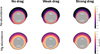 |
Fig. C.1 Same as figure 9 with Na and Mg abundances. |
| In the text | |
|
Fig. D.1 Corner plot of the single species retrieval with only VO |
| In the text | |
|
Fig. D.2 Corner plot of the full retrieval analysis |
| In the text | |
Current usage metrics show cumulative count of Article Views (full-text article views including HTML views, PDF and ePub downloads, according to the available data) and Abstracts Views on Vision4Press platform.
Data correspond to usage on the plateform after 2015. The current usage metrics is available 48-96 hours after online publication and is updated daily on week days.
Initial download of the metrics may take a while.