| Issue |
A&A
Volume 687, July 2024
|
|
|---|---|---|
| Article Number | A119 | |
| Number of page(s) | 21 | |
| Section | Planets and planetary systems | |
| DOI | https://doi.org/10.1051/0004-6361/202348879 | |
| Published online | 03 July 2024 | |
Atmospherix
III. Estimating the C/O ratio and molecular dynamics at the limbs of WASP-76 b with SPIRou★
1
IRAP, UMR5277 CNRS, Université de Toulouse, UPS,
Toulouse,
France
e-mail: This email address is being protected from spambots. You need JavaScript enabled to view it.
2
Department of Physics, University of Oxford,
Oxford
OX1 3RH,
UK
3
Université Paris-Saclay, UVSQ, CNRS, CEA,
Maison de la Simulation,
91191
Gif-sur-Yvette,
France
4
Université Côte d’Azur, Observatoire de la Côte d'Azur, CNRS,
Lagrange, CS
34229,
Nice,
France
5
Université Grenoble Alpes, CNRS, IPAG,
38000
Grenoble,
France
6
Université de Paris Cité and Univ Paris Est Creteil, CNRS, LISA,
75013
Paris,
France
7
LESIA, Observatoire de Paris, Université PSL, Sorbonne Université, Université Paris Cité, CNRS,
5 place Jules Janssen,
92195
Meudon,
France
8
Institut d’Astrophysique de Paris, CNRS, UMR 7095, Sorbonne Université,
98 bis bd Arago,
75014
Paris,
France
9
Laboratório Nacional de Astrofísica,
Rua Estados Unidos 154,
37504-364,
Itajubá,
MG,
Brazil
10
Laboratoire de Météorologie Dynamique/IPSL, CNRS, Sorbonne Université, Ecole Normale Supérieure, Université PSL, Ecole Polytechnique, Institut Polytechnique de Paris,
75005
Paris,
France
11
Laboratoire d’astrophysique de Bordeaux, Univ. Bordeaux, CNRS,
B18N, allée Geoffroy Saint-Hilaire,
33615
Pessac,
France
Received:
7
December
2023
Accepted:
22
March
2024
Abstract
Measuring the abundances of C- and O-bearing species in exoplanet atmospheres enables us to constrain the C/O ratio, which contains indications about the planet formation history. With a wavelength coverage going from 0.95 to 2.5 µm, the high-resolution (R ~ 70 000) spectropolarimeter SPIRou can detect spectral lines of major bearers of C and O in exoplanets. Here, we present our study of SPIRou transmission spectra of WASP-76 b acquired for the ATMOSPHERIX programme. We applied the publicly available data analysis pipeline developed within the ATMOSPHERIX Consortium, analysing the data using 1-D models created with the petitRADTRANS code, with and without a grey cloud deck. We report the detection of H2O and CO at a Doppler shift of around −6 km s−1, which is consistent with previous observations of the planet. Finding that a deep cloud deck is favoured, we measured a mass mixing ratio (MMR) log(H2O)MMR = −4.52 ± 0.77 and log(CO)MMR = −3.09 ± 1.05 consistent with a sub-solar metallicity to more than 1σ. We report 3σ upper limits for the abundances of C2H2, HCN, and OH. We estimated a C/O ratio of 0.94 ± 0.39 (~ 1.7 ± 0.7 × solar, with errors indicated corresponding to the 2σ values) for the limbs of WASP-76 b at the pressures probed by SPIRou. We used 1-D ATMO forward models to verify the validity of our estimation. Comparing them to our abundance estimations of H2O and CO, as well as our upper limits for C2H2, HCN and OH, we found that our results were consistent with a C/O ratio between 1 and 2 × solar, and hence with our C/O estimation. Finally, we found indications of asymmetry for both H2O and CO when investigating the dynamics of their signatures, pointing to a complex scenario possibly involving both a temperature difference between limbs and the presence of clouds being behind the asymmetry that this planet is best known for.
Key words: methods: data analysis / techniques: spectroscopic / planets and satellites: atmospheres / planets and satellites: individual: WASP-76 b
Based on observations obtained at the Canada–France–Hawaii Telescope (CFHT), which is operated from the summit of Maunakea by the National Research Council of Canada, the Institut National des Sciences de l’Univers of the Centre National de la Recherche Scientifique of France, and the University of Hawaii. The observations at the Canada-France–Hawaii Telescope were performed with care and respect from the summit of Maunakea, which is a significant cultural and historic site.
© The Authors 2024
 Open Access article, published by EDP Sciences, under the terms of the Creative Commons Attribution License (https://creativecommons.org/licenses/by/4.0), which permits unrestricted use, distribution, and reproduction in any medium, provided the original work is properly cited.
This article is published in open access under the Subscribe to Open model. This email address is being protected from spambots. You need JavaScript enabled to view it. to support open access publication.
1 Introduction
With thousands of exoplanets now discovered, a major next step in their study is the characterisation of their atmospheres. In doing so, we can obtain information about their chemical and physical properties. This has already been performed for over a hundred planets1 using data acquired using space-based and/or ground-based telescopes (see, notably, a review in Guillot et al. 2023, as well as the first results from James Webb: Taylor et al. 2023; JWST Transiting Exoplanet Community Early Release Science Team 2023). Such information can help to constrain the scenarios in which the exoplanets formed and evolved in time (e.g. Madhusudhan et al. 2017).
Transmission spectroscopy is an important tool in the characterisation of exoplanetary atmospheres. The variations in stellar light due to absorption by the atmosphere of an exoplanet as it passes in front of its host star result in spectra that contain information on both the temperature and chemical properties of the atmosphere at the limbs of the exoplanet (commonly referred to as morning and evening). From the measured properties as well as any differences between the morning and evening limbs, properties concerning the 3-D structure of the atmosphere can be inferred (Pluriel 2023). From the ground, the Doppler shift of a planet observed with high-resolution spectroscopy also enables the inference of dynamical processes in the atmosphere (e.g. Snellen et al. 2010; Flowers et al. 2019).
One of the most recent near-infrared (nIR), ground-based, high-resolution instruments is SPIRou (Spectro-Polarimètre InfraRouge; Donati et al. 2020), a fibre-fed cryogenic échelle spectrograph. Installed at the Canada–France–Hawaii Telescope in 2018, it has been observing the sky since 2019. SPIRou observes in the near-infrared, with a continuous coverage from 0.95 to 2.5 µm provided by 49 overlapping diffraction orders. With a resolving power of R ~ 70 000 and a sampling precision level of ~2.27 km s−1 per pixel, SPIRou is one of the best instruments to study volatile species in exoplanetary atmospheres. It has already been successfully used to do so for τ Boob (Pelletier et al. 2021), HD 189733 b (Boucher et al. 2021; Klein et al. 2024) and WASP-127 b (Boucher et al. 2023).
To best exploit the SPIRou observations of exoplanetary atmospheres, the ATMOSPHERIX programme (PI: Florian Debras) was created. With a consortium made up of a large French community of specialists in exoplanet atmospheric and stellar observations and simulations, its main goal is to use high-resolution observations to obtain knowledge on exoplanet atmospheric properties. To do so, a pipeline has been developed within the consortium to analyse high-resolution spectroscopic data, optimised for SPIRou data (Klein et al. 2024; Debras et al. 2024). Within the programme, data concerning 14 exo-planets have so far been acquired, including data concerning WASP-76 b.
WASP-76 b (West et al. 2016) is an ultra-hot Jupiter (UHJ) with a reported equilibrium temperature of approximately 2200 K. Having been observed with both space- and ground-based instruments, a variety of atomic and molecular detections have been reported for the atmosphere of this planet. Data acquired with HST have led to detections of H2O and Na and, tentatively, TiO and VO (Tsiaras et al. 2018; Fisher & Heng 2018; von Essen et al. 2020; Edwards et al. 2020; Fu et al. 2021). Furthermore, Spitɀer data showed a strong CO emission feature (Fu et al. 2021). Sodium has also been detected using data from HARPS (Seidel et al. 2019; Žák et al. 2019), ESPRESSO (Tabernero et al. 2021; Kesseli et al. 2022; Azevedo Silva et al. 2022), Subaru/HDS (Kawauchi et al. 2022), MAROON-X (Pelletier et al. 2023), and GRACES (Deibert et al. 2023). The ESPRESSO data were also used to detect Li, Mg, Ca+, Mn, K, Fe, V, Cr, Ni, Sr+, Ba+; and, tentatively, H, K, and Co (Ehrenreich et al. 2020; Tabernero et al. 2021; Kesseli et al. 2022; Azevedo Silva et al. 2022; Gandhi et al. 2022). HARPS data also led to the detection of Fe (Kesseli & Snellen 2021). Detections of Ca+ and Fe were also made using GRACES, as well as tentative detections of Li, K, Cr, and V (Deibert et al. 2021, 2023). MAROON-X data also led to detections of Fe, Ca+, Cr, Li, H, V, VO, Mn, Ni, Mg, Ca, K, and Ba+; tentatively detected O and Fe+ ; and revealed possible evidence of cold trapping of materials on the night side of the planet (Pelletier et al. 2023). CARMENES transmission data has led to reported detections of Ca+, OH, HCN, H2O, and, tentatively, NH3 (Casasayas-Barris et al. 2021; Landman et al. 2021; Sánchez-López et al. 2022). Emission data obtained with CRIRES+ led to a detection of CO (Yan et al. 2023). We summarise the different detections for WASP-76 b in Table A.1. There are currently no published papers retrieving abundance values for both water and CO for the atmosphere of WASP-76 b, though a similar study to this one was started using IGRINS data, with the first results presented at Exoplanets IV (see poster presentation of Mansfield et al. 2022). The iron detection by Ehrenreich et al. (2020) showed an asymmetry between the morning and evening terminators of WASP-76 b. The detection signal seemed to indicate iron present on the evening limb of the planet but absent on the morning side. This asymmetric iron signal was confirmed by Kesseli & Snellen (2021) using archival HARPS data. Different explanations were given for this phenomenon; Ehrenreich et al. (2020) put forward a condensation of iron on the night-side of the planet leading to a lack of iron on the morning side, while Wardenier et al. (2021) and Savel et al. (2022) showed that it could also be explained by a substantial temperature asymmetry between limbs and the presence of high-altitude optically thick clouds on the morning terminator, respectively.
In this paper, we present our analysis of SPIRou-acquired data concerning WASP-76 b. We first describe the WASP-76 b data acquired by SPIRou and the reduction process used in preparation for its analysis in Sect. 2. We then describe the models and methods with which these reduced data were analysed in Sect. 3. The results are presented in Sect. 4, including, notably, molecular detections and dynamical effects. Finally, we discuss these results in Sect. 5, giving an estimate of the C/O ratio of the planet. Section 6 features our conclusion.
2 Observations and data reduction
2.1 Observations
The UHJ WASP-76 b was observed as part of the ATMO-SPHERIX programme during the night of 31 October 2020. Lasting approximately 6 h, the observation consisted of 28 exposures and captured a full transit of the planet, with the first four and last seven being out-of-transit exposures and those in between being in-transit exposures. The second spectrum was removed due to this second exposure having been aborted; it had an integration time of only 33.432 s (with 774.497 s being the requested integration time). The remaining 27 spectra were used for our study. The adopted parameters of the observed star-planet system are listed in Table 1. Over the whole observation, the peak signal-to-noise ratio (S/N) per 2.3 km s−1 velocity bin varies between 127 and 167 (with a mean of ~161), and the air mass varies between 1.05 and 1.45. The transit curve and the variations in air mass, the radial correction values, and the registered peak S/N values over the different exposures can be seen in Fig. 1.
2.2 Data reduction
The data obtained of WASP-76 b were reduced using version 0.6.132 of APERO (A PipelinE to Reduce Observations), SPIRou’s data-reduction software (DRS; Cook et al. 2022). APERO applies the optimal extraction method of Horne (1986) to extract each individual exposure from the H4RG detector (Artigau et al. 2018). The wavelength solution is obtained by combining calibration exposures of a UNe hollow-cathode lamp and a thermally stabilised Fabry-Pérot etalon (Bauer et al. 2015; Hobson et al. 2021). APERO performs a correction of the telluric contamination using a method (summarised in Cook et al. 2022, see Sect. 8) that will be presented in a forthcoming paper (Artigau et al., in prep.). This technique applies TAPAS (Bertaux et al. 2014) to pre-clean telluric absorption, and the low-level residuals are removed using a data set of spectra of hot stars observed in different atmospheric conditions to build a residual model as a function of a few parameters (optical depths of H2O and of dry components). We note that the deepest telluric lines (relative absorption larger than 90%) are masked out by the pipeline as the low amount of transmitted flux will most likely result in an inaccurate telluric correction. Our input sequence of spectra contains the blaze-and telluric-corrected spectra. As the quality of this telluric correction improves with the number of epochs used to create the correction template and there have been fairly few observations of WASP-76 b, there is a high probability of telluric contamination remaining in the spectra.
We then applied the ATMOSPHERIX pipeline2 to reduce transmission spectroscopy data (Klein et al. 2024). It is made up of different steps, summarised as follows.
- 1.
The spectra are all aligned in the stellar rest frame, from which a master-out spectrum Iref is created by averaging out-of-transit exposures. This master-out spectrum is then moved back to the geocentric frame and linearly matched in flux to each of the observed spectra, which are each divided by its best-fitting solution. The resulting spectra are then divided by a second master-out spectrum, created by averaging the out-of-transit parts of these spectra, now in the Earth rest frame, to provide an additional correction of the tellurics. The option of correcting for planet-induced distortions of the stellar line profile (Chiavassa & Brogi 2019) was not used, as the star has a low rotational velocity.
- 2.
A normalisation of each of the resulting spectra is then performed using an estimate of the noise-free continuum, calculated using a rolling mean window. This is followed by a 5σ clipping being applied to remove outliers. This two-step process is then repeated until there are no more outliers flagged in the data.
- 3.
As some pixels with high temporal variance might remain, we calculated the variance for each pixel and applied an iterative parabolic fit to the pixel variance distribution. We considered pixels further than 5σ from the fit as outliers and masked them out for the rest of the data-reduction process.
- 4.
This step is optional. It is possible to detrend with the geometric air mass in log space according to Brogi et al. (2018). We chose to use it, performing a quadratic detrending of the resulting spectra, as it provides an additional correction for residual tellurics.
- 5.
Finally, we further correct remaining correlated noise through the use of a principal component analysis (PCA). The number of principal components (PC) to remove per order is automatically chosen by comparing the PC eigenvalues to the variance of a map of white noise with similar dispersion as our data. PCs with eigenvalues larger than the white noise mean eigenvalue are discarded. For our WASP-76 b data, between one and three PCs were removed for each order.
Unfortunately, applying a PCA to the data also affects the planetary signal, degrading it. Previous works have tried to take into account (at best) this effect so as to optimise the analysis of the data (Brogi & Line 2019; Gibson et al. 2020; Boucher et al. 2021; Pelletier et al. 2021). To take into account the degradation of our data of WASP-76 b, we implemented the method of Gibson et al. (2022), it being the fastest PCA method. For this, during the data-reduction process, we keep a matrix U of the removed eigenvectors for each order; this is assumed to be associated with correlated noise. These are subsequently used to prepare the synthetic spectra for analysing the data to degrade them coherently with the real signal (see Sect. 3.1).
Adopted WASP-76 system parameters.
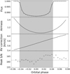 |
Fig. 1 Continuum-normalised light-curve, air mass, radial velocity (RV) correction (containing RV contributions of the barycentric Earth motion and the stellar systemic velocity), and peak S/N per velocity bin over the course of the transit of WASP-76 b as a function of the orbital phase (from top to bottom), computed using the parameters listed in Table 1. The grey band indicates the transit duration of the planet, from first to fourth contact. The horizontal dashed line in the bottom panel represents the average value of the peak S/N. |
3 Methods
Though the aim of the data-reduction process is to minimise the correlated noise, the atmospheric signal remains buried in noise. To extract it, we used synthetic spectra, cross-correlating them with the reduced data. We also used these synthetic spectra to investigate limits to our detection capabilities for the atmospheric properties of WASP-76 b.
3.1 Models
The models we used to analyse our reduced data were created using the petitRADTRANS Python package (Mollière et al. 2019, 2020). petitRADTRANS can be used to generate both emission and transmission spectra, at either low resolution (λ/Δλ ≤ 1000) or high resolution (λ/Δλ = 106). The modelled spectra can be produced for both clear and cloudy atmospheres. To make transmission spectra, it assumes the temperature and abundance profiles to be one-dimensional (1-D) and to describe the vertical structure of the entire planet. It also uses some properties of the star-planet system for which the adopted values are given in Table 1. When creating the spectra, we set up an atmosphere with 130 pressure layers going from 10−8 to 102 bars (each being equidistant in log space), with a reference pressure of P0 = 0.1 bar defining the base of our atmosphere. We included the Rayleigh scattering cross-sections of H2 and He, as well as the collision induced absorption cross-sections for the H2–H2 and H2–He pairs. Clouds are included as a grey cloud deck at a given pressure. Assuming a solar H/He ratio, we also used molecular line lists of H2O (Polyansky et al. 2018), CO (Rothman et al. 2010; Kurucz 1993), C2H2 (Rothman et al. 2013), HCN (Harris et al. 2006; Barber et al. 2014), and OH (Rothman et al. 2010). Abundances in petitRADTRANS are in mass-mixing ratios (MMRs). For all models used for our analysis, we assumed a vertically isothermal profile, as well as a uniform composition for the atmosphere.
Before using these models to analyse our reduced data, we wanted to bridge the gap between our model spectra and the real signal in terms of resemblance. First, UHJ are expected to have circular orbits and be tidally locked (see a review in Baraffe et al. 2010), assumptions that lead to an estimated rotation speed of ~5200 m s−1 at the equator of WASP-76 b. Rotational broadening will thus have a non-negligible effect on the spectral features. To take into account the effect of rotation, we used the double convolution framework presented in Klein et al. (2024), which allowed a statistical exploration of rotation speed; we discuss this in the following sections. Other sources of broadening are the instrumental precision and exposure time, taken into account by convolving the signal with, respectively, a Gaussian function and a window function that averages the planet velocity over its ~ 6200 m s−1 motion during the ~ 774 s integration time of each exposure. After broadening our petitRADTRANS model spectra, we normalised them. This is to replicate the normalisation of the real data during the reduction process described in Sect. 2.2.
We also needed to take into account the effects from the orbital motion of WASP-76 b on the spectral features. For this, we first modulated the spectra by the transit window shown in Fig. 1 to recreate the variations in intensity as the planet passes in front of its star. We then Doppler-shifted the modelled spectra by the planet radial velocity, Vp, calculated for each phase ϕ of the observation (with ϕ itself calculated using the mid-transit time, the time vector of each exposure, and the orbital period). As we kept the observed data in the geocentric frame, we calculated Vp in the same frame considering the orbit of WASP-76 b to be circular and by taking into account the barycentric Earth RV (BERV), and the stellar RV:
 (1)
(1)
with Kp being the planet’s radial velocity semi-amplitude, V0 the planet’s systematic Doppler shift, and Vc the stellar radial velocity.
As mentioned in Sect. 2.2, the models also needed to be degraded coherently with the degradation of the signal due to the PCA to accurately represent the real atmospheric signal present in our reduced data. We followed the method of Gibson et al. (2022), our final modified degraded model M being calculated for each phase as follows:
 (2)
(2)
with M and U corresponding to our non-degraded model and the matrix stored during the data reduction process (U† being its pseudo-inverse), respectively.
3.2 Analysis
3.2.1 Cross-correlation maps
Cross-correlation maps are made by cross-correlating the reduced data with the modelled spectra, over a large range of Kp and V0 values used in Eq. (1). Such maps allow the detection of an atmospheric signal by finding a maximal correlation value around the physically expected Kp and V0 values for the planet. The former can be calculated using the mass values of the star and planet, and the semi-amplitude of the stellar RV. The latter is informed by previous studies of WASP-76 b’s atmospheric signal such as Ehrenreich et al. (2020) and priors for atmospheric dynamics in exoplanet atmospheres. The correlation function used is defined as in Boucher et al. (2021), as follows:
 (3)
(3)
where di represents the observed flux, mi the modelled spectra, and σi the flux uncertainty, with the index i corresponding to the pixel at time t and wavelength λ. We calculated the cross-correlation maps for values of Kp going from 0 to 300 km s−1 with a step of 2 km s−1, and of V0 going from −100 to +100 km s−1 with a step of 0.5 km s−1. The resulting correlation values are converted to significance of detection by dividing the former by the standard deviation of the areas considered to be dominated by white noise. We used theoretical values from Ehrenreich et al. (2020) for both Kp and V0 to mark approximately where the correlation is expected to peak within the map if the atmospheric signal is detected. As the Kp measured seems dependent on species (see Table 2 in Kesseli et al. 2022, for example), we chose to use Kp = 196.52 km s−1 (estimated neglecting atmospheric dynamics), though we expect to see a shift of up to approximately ΔKp = ±20 km s−1 (Wardenier et al. 2023). For the Doppler shift, we used V0 = −5.3 km s−1, a value assumed for the day-to-night wind velocity in Ehrenreich et al. (2020) to compensate the redshift due to planet rotation for the morning limb.
Priors used in our nested sampling algorithm through this paper, and posteriors found in Sects. 4.1 (Post. 1), 4.2 (Post. 2), 4.3 (Post. 3), 4.4 (Post. 4), and 5.1.2 (Post. 5).
3.2.2 Atmospheric retrieval
To search for the best-fit values of our parameters, we used two methods. The first was a Markov chain Monte Carlo (MCMC) algorithm using the emcee python module (Foreman-Mackey et al. 2013). The second was a nested sampling (NS) algorithm using the python module pymultinest (Buchner et al. 2014). As in Klein et al. (2024), we found the latter to be around 50 times faster than the former while giving very similar results. For these reasons, we only present the results from the NS algorithm. Our choice of priors for this whole paper are summed up in Table 2.
For our parameter search, we used the likelihood 𝓛 defined in Gibson et al. (2020) by
 (4)
(4)
where α and β are scaling factors that take into account scale uncertainties of the model and the white noise, respectively. Tests of leaving α as a free parameter for models containing only H2O opacity lines showed a preference for α = 1 and a slight degeneracy with temperature (as α increased, the temperature decreased) coming from the fact that both parameters influence the scale height. For the rest of our study, we chose to set α = 1, as in Brogi & Line (2019), which implies that the scale of the model is the same as the analysed data. When including β within our free parameter set, we found very similar results as we did when setting β = 1. As the main difference between the former and the latter was computational cost, with the latter being around 2 × faster than the former, we chose to set β = 1.
3.2.3 Data simulator
We also used the petitRADTRANS generated spectra to simulate SPIRou observations of the atmospheric signal of WASP-76 b. The models were created and broadened following the same procedure as described in Sect. 3.1. They were then injected into our real data at a negative Kp value so as not to confuse our simulated signal with the real signal. We also chose to inject them at V0 different from that expected for the real signal. The noise level for our simulated data was hence the same as that for the real atmospheric signal.
The data containing our simulated spectra were then put through the data reduction pipeline described in Sect. 2.2 and analysed through the use of cross-correlation maps as described in Sect. 3.2.1. Unlike for the real atmospheric signal, we know the exact input parameters of the atmospheric signal that we are searching for. Thus, a non-detection of the simulated signal would indicate a too high noise level to allow a detection. Hence, we can investigate the required abundances of different species that could be in the atmosphere for a detection to be possible.
3.3 Forward models
We used the 1-D radiative-convective chemical equilibrium code ATMO (Tremblin et al. 2015; Amundsen et al. 2014; Drummond et al. 2019) to create forward models of the atmosphere ofWASP-76 b. As for creating the petitRADTRANS model spectra, we set the number of pressure layers to 130, going from around 10−8 to 102 bar. The pressure-temperature profiles for these models are calculated by ATMO to satisfy both hydrostatic equilibrium and conservation of energy. Physically consistent chemical abundance profiles of 175 gaseous species are also calculated by the code in equilibrium from solar abundances of 23 elements (H, He, C, N, O, Na, K, Si, Ar, Ti, V, S, Cl, Mg, Al, Ca, Fe, Cr, Li, Cs, Rb, F, and P, with abundances adopted from Caffau et al. 2011). As we could change the C/O ratio of the modelled atmosphere by modifying the initial quantities of C and/or O, we created models with the same C/O ratio obtained for different initial abundances of C and O. We first used these forward models to predict which species were the most likely to be present in the atmosphere and detectable with SPIRou. We then later used these same forward models to evaluate if the (non-)detections of these species and the abundance values or upper limits retrieved with the NS algorithm were coherent with the estimated C/O ratio.
4 Results
Using ATMO forward models, we estimated that depending on the C/O ratio, the most probable species to be present in the atmosphere that can be detected with SPIRou are H2O, CO, HCN, C2H2 and OH. This section therefore presents our attempts to detect them and the associated temperature, cloud, and dynamical profiles recovered.
4.1 H2O and CO
To first detect WASP-76 b’s atmosphere, we used models created following the procedure described in Sect. 3.1 including only water opacity lines, with log(H2O)MMR = −5.0. We used an isothermal temperature profile with T = 1500 K, a choice motivated by the retrieval results obtained using our NS algorithm presented later in this section. The resulting cross-correlation map can be seen in Fig. 2. The maximum S/N of 7.29 was obtained for Kp = 180 km s−1 and V0 = −6.0 km s−1. The intersection of the theoretical values from Ehrenreich et al. (2020) are within the 1σ boundary of our maximum S/N peak. Furthermore, Wardenier et al. (2021) showed that 3-D effects in the atmosphere of WASP-76 b such as atmospheric dynamics and rotation can lead to a shift in Kp up to 30 km s−1 lower than the expected value. This has previously been observed for many of the detected species reported in Table A.1, with the measured shift changing depending on the species (e.g. Kesseli etal. 2022; Deibert et al. 2023). We were hence able to confirm both the detection of the atmosphere of WASP-76 b and the presence of H2O in its atmosphere.
We next looked for an atmosphere assumed to only contain CO. The models were createdas described in Sect. 3.1, with only CO opacity lines included (log(CO)MMR = −4.0). The resulting cross-correlation map can be seen in Fig. 3, also confirming a detection of CO in the atmosphere, dynamically consistent at 1σ with the H2O detection but only consistent at 2σ with the values from Ehrenreich et al. (2020).
We were then able to estimate abundances for both H2O and CO using our NS algorithm. The output parameters were the orbital RV semi amplitude, the Doppler shift, the abundance of water and CO, the temperature, and the cloud-top pressure as shown in Table 2. The presence of high-altitude clouds in the atmosphere can impact the absorption-line depth and hence the measurement of chemical abundances. The resulting posterior distributions are presented in Appendix E. The maximum posterior probabilities give a temperature of 1355 ± 313 K, with 1σ error bars, much colder than the mean temperature obtained by Pelletier et al. (2023) for transit observations in the visible (∽3000 K). However, when comparing our isothermal temperature profile to the vertical temperature structure found by Pelletier et al. (2023) (see Fig. 4), we can see that we are closest in temperature for a pressure of around 10−4 bar. This is coherent with the higher sensitivity of SPIRou data to pressure levels going from around 10−4 to 10−2 bar. The MMR of water, −4.53 ± 0.77 (in log), is about ten times lower than that of CO (−3.10 ± 1.05). This translates into a C/O ratio of 0.94 ± 0.15, which is discussed further in Sect. 5. The data favour either a deep cloud deck or, more likely, the absence of clouds, excluding clouds higher than 10−4 bars at 3σ. We can see two expected degeneracies: temperature with abundances as well as cloud-top pressure and abundances. As we show in Sect. 5, these degeneracies mostly affect the metallicity while keeping a C/O ratio roughly constant. Because water and CO could be sensitive to different pressure levels in the atmosphere and that that would affect their recovered abundances when retrieving them jointly, we also ran NS algorithms with only each of these molecules included. The retrieval of water is globally unchanged, while we find a higher quantity of CO (−2.74 ± 0.95) linked to a temperature 300 K higher (not shown). This further confirms a high C/O ratio (Sect. 5).
As water is detected more strongly than CO, it also has a higher influence on the likelihood. In that regard, while we were able to obtain a lower limit for water, the data are consistent with the absence of CO at 3σ. However, we know that CO is present in the atmosphere, as shown by our detection in Fig. 3 and other studies. Hence, this acts as a bias towards lower abundances of CO and, by extension, lower recovered C/O values in the atmosphere.
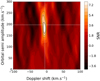 |
Fig. 2 Map resulting from cross-correlation between reduced data of WASP-76 b and spectra from a model containing H2O opacity lines. The S/N varies from -3.86 to 7.29, with the maximum peak in S/N of 7.29 obtained for Kp = 180 km s−1 and V0 = −6.0 km s−1. The black lines (full, dashed and dotted), respectively, represent the 1, 2, and 3 σ contours. The white dashed lines represent the theoretical values from Ehrenreich et al. (2020) of Kp = 196.52 km s−1 and V0 = −5.3 km s−1. |
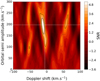 |
Fig. 3 Same as Fig. 2, but using models containing only CO. The S/N varies from -3.30 to 5.03. The maximum S/N was obtained for Kp = 200 km s−1 and V0 = −11.5 km s−1. |
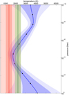 |
Fig. 4 Temperature profile from extended data Fig. 5 in Pelletier et al. (2023) (blue) compared to the isothermal temperature profile from Fig. 7 in Edwards et al. (2020) (green) and the isothermal temperature profile retrieved in Fig. E.1 with T = 1355 K (red), with the shaded regions representing the 1 and 3σ error bars (only 1σ represented for the profile from Edwards et al. 2020). |
4.2 HCN and C2H2
Other species we estimated to potentially be present in the atmosphere of WASP-76 b are HCN and C2H2. However, we were unable to detect either of these species when analysing the data of WASP-76 b. Nevertheless, we were able to infer upper limits of their abundances from the results of the atmospheric retrieval (see Fig. H.1), with these roughly indicating log(C2H2)MMR < −5.0 and log(HCN)MMR < −5.5.
We used the data simulator (see Sect. 3.2.3) to verify the limitations of our detection for these two species in our data. The simulated atmospheric signals used contained both water (with log(H2O)MMR = −5.0) and either HCN or C2H2 with different MMRs. Each was analysed using a model containing only the species included in the simulated signal, either HCN or C2H2, with the same MMR as that used to create the signal. We found that for C2H2, an MMR of 10−6 was required for any indications of a detection, while for HCN, an MMR of 10−4 was needed. This is somewhat in agreement with the upper limits previously inferred from the nested sampling algorithm results. We further discuss these results in Sect. 5.1.3.
4.3 OH
The hydroxyl radical OH has been detected in the atmosphere of WASP-76 b (Landman et al. 2021; Mansfield et al. 2022). However, we were not able to detect it in our data. An upper limit for the abundance was indicated by the NS algorithm results, roughly indicating log(OH)MMR < −6 (see Fig. H.2). With the data simulator, we were able to infer that a detection would be possible for log(OH) ≳−4. We also used the data simulator with the telluric-corrected data from the APERO version 0.7.275 to investigate the detectability of OH, as this later version of the SPIRou DRS is supposed to have an improved correction for OH signal coming from looking through the Earth’s atmosphere. However, we also found that a log(OH)MMR of at least −4 was required for a detection to be possible, finding the same detection limit for OH as found for the data from version 0.6.132 of APERO.
4.4 Dynamics
To investigate the rotational velocity of the planet, we used cloud-free models for which we fixed the temperature to T = 1500 K and included both H2O and CO opacity line lists. The NS algorithm results can be seen in Appendix F. The Kp and V0 values found are in good agreement with those found in Sect. 4.1, being within 1σ of those values. The abundances found for both water and carbon monoxide are lower than those previously found in Sect. 4.1, but consistent at <1σ. The rotation velocity found of υeq = 3544 ± 1501 m s−1 is lower than that expected for WASP-76 b (estimated to be υeq,theoretical ≃ 5210 m s−1) by considering the planet as tidally locked and with a circular orbit. However, the expected velocity is within the 2σ boundaries (and actually very close to 1σ).
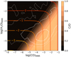 |
Fig. 5 Representation of possible C/O and [(C+O)/H] values for the posteriors of log(H2O) and log(CO). The white lines (full, dashed, and dotted), respectively, represent the 1, 2, and 3σ contours shown in Fig. E.1. For the whole range of possible values of log(H2O)MMR and log(CO)MMR, we calculated the corresponding values of the C/O and [(C + O)/H] ratios. The background represents the resulting values of C/O ratio. The coloured lines indicate the values of [(C+O)/H]. |
5 Discussion
5.1 C/O ratio
5.1.1 Estimation
We were not able to detect any C or O bearers other than H2O and CO. Forward models subsequently created with ATMO for different C/O ratios values showed that water and carbon monoxide are the main bearers of these elements. We hence concluded that the abundances retrieved for H2O and CO found in Sect. 4.1 to be sufficient to get a first approximation for the C/O ratio local to the section of WASP-76 b’s atmosphere observed in our data. To do so, we first converted the MMR abundance values to volume-mixing ratios (VMRs). The C/O ratio was then calculated as in Line et al. (2021), which is as follows
 (5)
(5)
with nCO and  representing, respectively, the VMRs of CO and H2O. Using the most likely values for the abundances of water and CO found by our NS algorithm in Sect. 4.1, we estimated a C/O ratio of approximately 0.94 ± 0.39 (~1.7 ± 0.7 × solar, with solar abundances taken from Asplund et al. 2009 and errors indicated being for 2σ values) for the part of the atmosphere probed by the SPIRou transmission data used for this study. The C/O ratios estimated using the retrieval results associated with Sects. 4.2–4.4 are all within 1σ of this value. Indeed, the inclusion of HCN and C2H2 leads to a C/O ratio of 0.93 ± 0.35, the inclusion of OH to a C/O ratio of 0.92 ± 0.21, and the use of cloud-free models to a C/O ratio of 0.93 ± 0.34 (with errors indicated corresponding to the 2σ values). Furthermore, we compared the sigma contours for the posterior values of [H2O, CO] to the C/O ratios calculated for the prior ranges of H2O and CO (see Fig. 5). For values within the 1σ boundary, we found C/O to be greater than 0.6 (~1.1 × solar). The other sigma contours, however, encompass all possible C/O values. This seems to be a direct consequence of the lack of a lower boundary for the abundance of CO. However, due to only including CO as a C-bearing species, Eq. (5) is naturally limited to vary between 0 and 1. This is furtherexplored in the nextsubsections.
 |
Fig. 6 Variations in VMR of H2O and CO depending on pressure calculated by ATMO for C/O = 0.5, 1,1.6, and 2 × solar. |
5.1.2 Robustness of a super-solar C/O ratio
We used the 1-D radiative–convective code ATMO (Tremblin et al. 2015) to investigate the expected abundance profiles of H2O and CO depending on the overall C/O ratio of the atmosphere. We note that unlike our C/O calculation with Eq. (5) that only uses abundances of H2O and CO, the C/O ratios of ATMO include all C- and O-bearing species included in the model. The results for C/O = 0.5, 1.0, 1.6, and 2.0 (× solar) can be seen in Fig. 6. From these results, we can infer that if C/O < 1 × solar, we would find log(H2O) > log(CO), while if C/O ~ 1 × solar, the measured abundances of H2O and CO would be of similar magnitude. We can also infer that if C/O was greater than 2× solar, then there would be several orders of magnitude between the abundances of water and CO. Hence, considering these results and the difference in order of magnitude found between the retrieved abundances of H2O and CO in Sect. 4.1, we would expect to estimate a C/O ratio greater than 1 × solar but smaller than 2× solar. This is consistent with our the C/O ratio estimated from our results, for which we assumed only H2O and CO present in the atmosphere.
Furthermore, it is shown in Line et al. (2013) that when using uniform or Gaussian priors for the abundances of the C and O bearing species, the corresponding calculated prior C/O ratio consists of two peaks, with a preference for a C/O ~ 1. To test for a possible bias on our estimated C/O ratio, we used uniform priors of C/O and [(C + O)/H] (a proxy for metallicity, with ‘[]’ referring to the log10 of the value relative to the solar value). As we consider once again only H2O and CO in the atmosphere, we impose an upper limit on possible C/O ratios of one. The calcula-tions of the corresponding abundances of H2O and CO are shown in Appendix C. The results obtained from the NS algorithm are shown in Appendix G. The maximum probability for the distribution of C/O is obtained for a value of  (with errors indicated here corresponding to 2σ values), which is roughly the same as the C/O ratio found using uniform distributions of H2O and CO as priors. We can see that similar degeneracies to those for water also exist for our metallicity proxy [(C + O)/H], being degenerate with temperature and cloud pressure. Meanwhile, the C/O ratio seems to remain relatively constant, though with a large lower boundary. This is consistent with what is shown by Fig. 5, with the large lower boundary on our estimation of C/O coming from the large lower boundary on the abundance of CO.
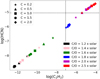 |
Fig. 7 Mean abundances in VMR of C2H2 and HCN (averaged over pressures from 100 to 10−4 bar). The black dashed lines correspond to the upper limit abundances found by the data simulator of log(C2H2)MMR = −6 and log(HCN)MMR = −4. |
5.1.3 Upper limits for HCN and C2H2
With ATMO, we calculated the abundance profiles of different species in thermochemical equilibrium. We did so for a variety of C/O ratios, which were obtained by changing the initial abundances of both C and O so as to also change the metallic-ity (Drummond et al. 2019). We estimated the expected quantity of HCN and C2H2 dependant on the C/O ratio (see Fig. 7). We compared the results to the upper limits found for these species to be detectable with the data simulator. Though the upper limit of HCN only excluded C/O ratio over 2.5 times solar, the upper limit of C2H2 excludes all C/O ratios that are above 1.8 × solar unless the metallicity is significantly sub-solar (see next section). This is in agreement with what was indicated previously by Fig. 6. Furthermore, C/O <1.8× solar is equivalent to C/O <0.99, which is consistent with our C/O value estimation from Sect. 5.1.1.
5.1.4 OH
Using the aforementioned ATMO models, we investigated the impact of our non-detection of OH on the C/O ratio as calculated using Eq. (5). In Fig. 8, we represent the mean abundance of OH for pressures probed by SPIRou as a function of the C/O ratio estimated using Eq. (5) for each of the ATMO models used. By comparing the results to the upper limit found using the data simulator, we can see that our non-detection of OH is also consistent with having a C/O ratio between 1 and 2 × solar for solar metallicity.
5.1.5 Implications on planet formation
Our different retrieval results all led to estimating the C/O ratio to be super-solar, finding C/O ∽ 0.9. This is in agreement with the super-solar C/O ratio found for transmission spectra acquired with HST by Fu et al. (2021) (−0.83 ± 0.76). However, neither our retrieval results nor those from Fu et al. (2021) exclude the sub-solar and solar C/O ratio cases entirely. Furthermore, while the upper limits found for C2H2, HCN, and OH seem to exclude the sub-solar C/O ratio case for solar metallicity, they do not exclude a solar C/O ratio for solar metallicity, or a sub-solar C/O ratio for a significantly sub-solar metallicity. Therefore, we cannot reasonably use our current results to place constraints on the formation scenario of this planet. By combining data from different transits in a future work, we should, however, obtain much better constraints on our abundances, and we will then also be able to constrain the planet formation scenario of WASP-76 b.
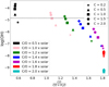 |
Fig. 8 Mean abundances in VMR of OH (averaged over pressures from 100 to 10−4 bar) as a function of the corresponding C/O ratio as estimated using Eq. (5). The black dashed line corresponds to the upper limit abundance found by the data simulator of log(OH)MMR= −4. |
5.2 Metallicity and clouds
Through our NS algorithm, we also looked at values calculated for [(C+O)/H], used as a proxy for metallicity (Fig. 5 and Appendix G). Our data favour sub-solar metallicity at 1σ while not excluding super-solar at 2σ, which prevents any solid conclusion on the metallicity. This is mainly due to the degeneracy with clouds, which prevents a robust estimation of the molecular mixing ratios.
As stated in Sect. 3.1, we included clouds as a grey cloud deck at a given pressure when considering a cloudy atmosphere for our atmospheric retrievals. Previous studies have also included a grey cloud deck in the models used for retrievals. Using HST transmission data, Edwards et al. (2020) retrieved a cloud pressure of log(Pclouds) = 0.91 ± 0.58 Pa (=−4.09 ± 0.58 bar). However, Pelletier et al. (2023) obtained a cloud-top pressure for their optically thick grey cloud deck of log(Pclouds) = −2.21 ± 0.28 bar using high-resolution optical transmission data from MAROON-X. Neither of these values correspond to the one found to be most probable by our NS algorithm, which favour a clear atmosphere, though neither are excluded. Coupling low- and high-resolution spectroscopic data might lift this degeneracy and allow us to conclude on the actual metallicity of the planet (Boucher et al. 2023).
Kp and V0 values for maximum S/N position obtained for water detection in each transit half.
5.3 Dynamics
5.3.1 H2O
In Sect. 4.1, we state that we obtained a Doppler shift of −6.0 km s−1 for the cross-correlation map of H2O. While this value is inconsistent with the value previously reported for H2O by Sánchez-López et al. (2022) (V0 ∽ −14.3 km s−1), it is consistent with both the value assumed for the day-to-night wind velocity from Ehrenreich et al. (2020) and measured Doppler shifts for other species detected in the atmosphere of WASP-76 b (e.g. Tabernero et al. 2021; Pelletier et al. 2023). This blueshift is hence compatible with a day-to-night wind of approximately the velocity measured, which is V0 = −6.0 km s−1. As this corresponds to the wind speed retrieved for the whole transit, this could imply an equal contribution from both limbs to the overall signal of H2O. However, with such a velocity having also been retrieved for species with asymmetrical signals such as iron (e.g. Tabernero et al. 2021; Pelletier et al. 2023), we cannot conclude from the cross-correlation map obtained for the whole transit of WASP-76 b on the asymmetry of the water signal. No further indications are given by looking at the 2-D cross correlation function map (see Appendix B).
To further investigate the asymmetry of H2O between the limbs of WASP-76 b, we looked at each half of the transit separately, similarly to Gandhi et al. (2022) and Kesseli et al. (2022). First, we separated the transit in two halves, splitting it in the middle, and performed the data-reduction and cross-correlation procedures described in Sects. 2.2 and 3.2.1 on each (see Appendix D). We were hence able to obtain Kp and V0 values for each half of the transit (see Table 3), considering these to be first-order approximations of what would be obtained applying the same procedure as Gandhi et al. (2022) to the water signal. Our results for the first and second halves are consistent with those from Gandhi et al. (2022) for, respectively, the first and last quarters for the Fe signal. The Doppler shift obtained for the first half of the transit is consistent with what we previously obtained for the whole transit, with a blueshift that could correspond to a significant contribution to the signal coming from both limbs. As for the second half, our measurement is consistent with a Doppler shift approximately twice as blueshifted as for the first half, which could point to the signal being dominated by the trailing limb, where the combination of planetary rotation and day-to-night winds result in a greater blueshift. To further our analysis, we also computed the mean cross correlation functions for each half from the 2-D cross correlation function map, to perform a similar analysis to Kesseli et al. (2022). We used the results of our Gaussian fits to each of these mean functions to compare our results for H2O to those found by Kesseli et al. (2022), in particular reproducing the comparison between relative amplitude differences as a function of radial velocity difference (see Fig. 9). As before, our results are compatible with water having a similar asymmetry as Fe, with the signal from the trailing limb seeming stronger than that from the leading limb.
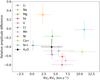 |
Fig. 9 Scatter plot showing relative amplitude difference as function of radial velocity difference between the first and second half of the transit from Kesseli et al. (2022), to which we added our results for H2O. |
5.3.2 CO
For CO, we found a peak centred at a higher velocity than for H2O, obtaining the maximum S/N for V0 = −11 5 km s−1. This velocity is compatible with the results found for the trailing limb by Ehrenreich et al. (2020) and Gandhi et al. (2022), which are within 1σ of the velocity measured by Ehrenreich et al. (2020). This could imply that the overall signal for CO is dominated by that from the trailing limb of the planet, with the measured Doppler shift resulting from the combination of the planetary rotation and day-to-night winds on that side of WASP-76 b.
Though we already found indications as to the asymmetry of the CO signal, we attempted nevertheless to further our analysis by looking at each half of the transit separately, as we previously did for H2O. However, we were unable to detect CO in eitherhalf separately. Additional data are required to have a sufficient S/N for each half to perform such a study for CO. We plan to revisit this analysis in a future work involving more transits observed by SPIRou of WASP-76 b.
5.3.3 Comparing to GCMs
In Wardenier et al. (2023), cross-correlation maps were given for different species (including H2O, CO and Fe) for different atmospheric models. We compared the resulting profiles to our results for H2O and CO, as well as the results obtained by Ehrenreich et al. (2020) and Kesseli et al. (2022) for Fe (as they use the same ESPRESSO dataset). For CO and Fe, the results were most compatible with the models where TiO and VO are cold-trapped and where there is a cold morning limb. As both of these species are expected to predominantly probe the day side (Wardenier et al. 2023) and both models have an asymmetry in temperature between limbs, these results point to a significant difference in temperature between the two limbs of WASP-76 b being behind the asymmetric signals of CO and Fe. As for H2O, a species expected to predominantly probe the night side (Wardenier et al. 2023), we found that our results were most consistent with the model involving optically thick clouds (see Fig. 10). However, the strength of our H2O signal and the results for clouds previously discussed in Sect. 5.2 could point to these optically thick clouds being lower in the atmosphere than for the model used by Wardenier et al. (2023) and/or these clouds being predominantly on the morning side of the planet. We note that due to the uncertainties on our results concerning H2O and CO, we cannot yet confirm the indications given here from our results as of the scenario corresponding to the atmosphere of WASP-76 b. Nevertheless, our results do point to this scenario being more complex than the ones from Wardenier et al. (2023), with it possibly being a combination of those different scenarios.
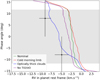 |
Fig. 10 Comparison between cross-correlation profiles for different scenarios for H2O obtained in Wardenier et al. (2023) and radial velocities we obtained for H2O from the mean cross-correlation functions for each half of transit. The ‘nominal’ profile (green) was obtained for a weak-drag model, the ‘cold morning limb’ profile (red) for a model for which the temperature was reduced on the leading limb, the ‘optically thick clouds’ profile (blue) for adding clouds as in Savel et al. (2022), and the ‘no TiO/VO’ profile (purple) for removing TiO and VO from the GCM calculations, considering them cold-trapped. The black dots correspond to the radial velocities obtained from Gaussian fits to the mean cross-correlation functions for each half of transit, the horizontal black bars corresponding to the associated errors, and the vertical black bars indicate the associated phase range. The grey band indicates the transit duration from post-ingress to pre-egress. |
6 Conclusion
We used the publicly available ATMOSPHERIX pipeline to analyse SPIRou-acquired transmission spectra of one transit of the UHJ WASP-76 b. Using models created with petitRADTRANS, we detected two major C- and O-bearing species -water and carbon monoxide- and measured their abundances local to the pressures probed by SPIRou for both cloudy and cloud-free models. Having included a grey cloud deck in our models, we found it to be favoured deep in the atmosphere, and measured log(H2O)MMR = −4.52 ± 0.77 and log(CO)MMR = −3.09 ± 1.05, leading to a C/O estimation of 0.94 ± 0.39 (~1.7 ± 0.7 x solar, with errors indicated corresponding to the 2σ values). For a cloud-free model, though we measured slightly lower abundances for H2O and CO than for with the inclusion of a grey cloud deck, we estimated a similar C/O ratio as for models with a grey cloud deck, finding C/O = 0.93 ± 0.34 (~ 1.7 ± 0.6 x solar). We also tried to detect HCN, C2H2, and OH, but we were only able to determine upper limits for their abundances.
These were consistent with upper limits of our detection capabilities for these species determined using the data simulator of the ATMOSPHERIX analysis pipeline. These cloud-free models were also in agreement with a local C/O of ~0.9. To account for possible biases coming from the use of uniform distribution for the abundances of H2O and CO as priors of our NS algorithm, we also used uniform distributions of C/O and [(C + O)/H] (a proxy for metallicity) as priors. However, we still found a preference for a C/O close to one, obtaining a maximum likelihood for  . Furthermore, with the abundance measurements of H2O and CO and the upper limits found for HCN, C2H2, and OH, we investigated the validity of our C/O ratio for the pressures probed by SPIRou using ATMO models. Overall, we found that the abundance measurements of H2O and CO and the upper limits determined for HCN, C2H2, and OH were consistent with a local C/O ratio between 1 and 1.8 × solar. This is thus consistent with our C/O ratio estimation for the pressures probed by SPIRou. However, the large uncertainties of our C/O estimation due to the large uncertainties of our CO abundance measurements preclude from reasonably placing constraints on the formation scenario of this planet.
Considering the famous Fe asymmetric signal of this planet found by Ehrenreich et al. (2020), we also investigated its dynamics. While the initial detection signal for CO pointed to carbon monoxide having a similar asymmetry to the one for iron, further investigation into each half of the transit was required for H2O. Nevertheless, we ultimately found an asymmetric signature for water that was also similar to the one for iron, though by comparing the results to GCM results, it became clear that these asymmetries could have different causes. Indeed, while the Fe and CO asymmetries indicated a temperature asymmetry, the explanation for the H2O asymmetry pointed to the presence of clouds. However, due to the large uncertainties of our results, additional data are required to confirm exactly which scenario is behind the asymmetries that have been found for species detected in the atmosphere of WASP-76 b. Nevertheless, our results do indicate that it could be a combination of temperature asymmetry and presence of clouds. Future work with JWST observations to measure the full 3-D temperature structure and cloud cover of the planet could hence be key to understanding the asymmetric signatures of WASP-76 b.
We were able to study the pressures probed by SPIRou at the full terminator of WASP-76 b, investigating the local C/O ratio and the dynamics of the corresponding pressure levels. By expanding this study to include data from other instruments, both ground- and space-based (such as JWST), acquired in transmission and emission, we could extend our local C/O estimation to one that is global to the planet. This could also lead to global estimations of other ratios such as Fe/O, which is used to constrain formation scenarios further than what is indicated by C/O.
Acknowledgements
F.D. thanks the CNRS/INSU Programme National de Plané-tologie (PNP) and Programme National de Physique Stellaire (PNPS) for funding support. F.D. acknowledges funding from the Centre National d’Etudes Spa-tiales in the context of the French participation to the ARIEL mission. B.K. acknowledges funding from the European Research Council under the European Union’s Horizon 2020 research and innovation programme (grant agreement no. 865624, GPRV). E.M. acknowledges funding from FAPEMIG under project number APQ-02493-22 and research productivity grant number 309829/2022-4 awarded by the CNPq, Brazil. This work was supported by the Action Spécifique Numérique of CNRS/INSU. This work was granted access to the HPC resources of CALMIP supercomputing center under the allocation 2021-P21021.
Data availability. The data are available upon request to the author and the code to analyse them is publicly available.
Appendix A Table of chemical species in WASP-76 b
In Table A.1, we show a list of chemical species that have been included in previous studies of the atmosphere of WASP-76 b. For each species, we indicate the instrument used to study its presence in the atmosphere of WASP-76 b, give the reference to the paper presenting the study, and state if it was reported as detected (highlighted green), tentatively detected (highlighted orange) or non-detected (highlighted red).
List of chemical species reported as detected (green), tentatively detected (orange), or not detected (red) in previous publications and this work. For each species has been indicated the instrument used and the corresponding reference for the study of its presence in the atmosphere. Empty cells indicate that the species has not been explicitly included in a published study with the corresponding instrument.
Appendix B Rest-frame absorption signals
Here we show the planetary rest-frame absorption trails for H2O and CO.
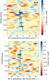 |
Fig. B.1 Cross-correlation trails for H2O (top) and CO (bottom). The dashed lines correspond to the absorption trails indicated for each species by the Kp and V0 values reported in Section 4.1. The black dotted lines correspond to the ’kinked’ absorption trail reported for Fe. The grey dotted horizontal lines correspond to the beginning and end of the transit. |
Appendix C Changing priors
As petitRADTRANS requires the abundance profile of a species when creatingmodel spectra,we had to derive the expressions to calculate the MMRs of H2O and CO from the expressions of the C/O and [(C+O)/H] (used as a proxy for metallicity). Considering only H2, H2O, and CO present in the atmosphere (equivalent to considering all other species negligible in the calculation of these ratios), we derived the following from these two ratios:
 (C.1)
(C.1)
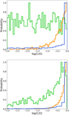 |
Fig. C.1 Distribution of log(C/O), with the top panel representing the priors and the bottom panel the posteriors. The blue lines correspond to when using uniform priors for the distributions of the MMRs of H2O and CO. The orange lines correspond to when using a uniform linear distribution of the C/O ratio. The green lines correspond to using a uniform distribution in log space of the C/O ratio. |
with Xi being the MMR of each species i included in the list of line absorbers, corresponding here to H2O and CO, which have the following expressions for Γi:
 (C.2)
(C.2)
![Mathematical equation: $\eqalign{ & {\Gamma _{CO}} = {{{\mu _{{H_2}}}} \over {{\mu _{CO}}\left( {1 - {H \over {He}}} \right)}} + {{C + O} \over H} + {{1 - {C \over O}} \over {{C \over O} \times {{{\mu _{CO}}} \over {{\mu _{{H_2}O}}}}}} \cr & \,\,\,\,\,\,\, \times \left[ {{{{\mu _{{H_2}}}} \over {2{\mu _{{H_2}O}}\left( {1 - {H \over {He}}} \right)}} + {{C + O} \over H} \times \left( {1 - {{{\mu _{{H_2}}}} \over {{\mu _{{H_2}}}o\left( {1 - {H \over {He}}} \right)}}} \right)} \right], \cr}$](/articles/aa/full_html/2024/07/aa48879-23/aa48879-23-eq45.png) (C.3)
(C.3)
with µi being the molecular mass of the species i (H2O, CO or H2), and using the solar H/He ratio (∽eq0.275).
The NS results can be seen in Figure G.1. We calculated the abundance probability distributions for H2O and CO from those of C/O and [(C+O)/H], finding a maximum probability for log(H2O)MMR = −4.27 ± 0.54 and log(CO)MMR = −3.48 ± 0.87. These values are both within 1 σ of those retrieved in Section 4.1.
We were also able to use a uniform prior of log(C/O) by replacing C/O with log(C/O) in Equations C.2 and C.3. In Figure C.1, wecomparethelog(C/O) distributions of both the priors and posteriors of each of our three cases (using uniform distributions of H2O and CO, of C/O and [(C+O)/H], and of log(C/O) and [(C+O)/H] as priors). We can see that only when using log(C/O) as prior do we not favour log(C/O) ∽ 0 as a posterior. However, by using a uniform distribution of log(C/O) as a prior, we also introduce a strong bias towards sub-solar values of C/O, and even extremely sub-solar values of C/O. Despite this strong bias, we still find that a solar value for C/O is most likely in this case. Taking into account the strong bias introduced by the chosen prior distribution, this seems to indicate a high likelihood of the C/O being super-solar, in agreement with what was found in our other two cases of study.
Appendix D Water detections in transit halves
Here, we show the maps resulting from the cross-correlation between each half of the transit of WASP-76 b and cloud-free models with T = 1500 K in which we included only H2O. Figure D.1 represents the resulting map for the first half of the transit. Figure D.2 represents the resulting map for the second half of the transit.
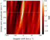 |
Fig. D.1 Map resulting from cross-correlation between reduced data of WASP-76 b from the first half of the transit and spectra from a model containing H2O opacity lines (log(H2O)MMR = −5.0), with T = 1500 K. The S/N varies from −3.16 to 4.65, with the maximum S/N of 4.65 obtained for Kp = 184 km s−1 and V0 = −4.5 km s−1. |
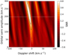 |
Fig. D.2 Map resulting from cross-correlation between reduced data of WASP-76 b from the second half of the transit and spectra from a model containing H2O opacity lines (log(H2O)MMR = −5.0), with T = 1500 K. The S/N varies from −3.39 to 4.75, with the maximum S/N of 4.75 obtained for Kp =216 km s−1 and V0 =−11.5 km s−1. |
Appendix E Retrieval results for H2O and CO abundance estimation
Here, we show the retrieval results associated with Section 4.1.
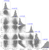 |
Fig. E.1 Corner plot showing NS results of our retrieval using WASP-76 b data. The black lines (full, dashed, and dotted) represent the 1, 2, and 3 sigma contours, respectively. The maximum probability and 1σ values found are represented for each histogram on the diagonal by the blue dot and bar. |
Appendix F Retrieval results for veq estimation
Here, we show the retrieval results associated with Section 4.4.
 |
Fig. F.1 Posterior distributions obtained from NS algorithm using cloud-free models with T = 1500K. Represented by the red dashed line is the expected rotation velocity for WASP-76 b (see Section 4.4). |
Appendix G Retrieval results for C/O ratio and metallicity
Here, we show the retrieval results associated with Section 5.1.2.
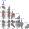 |
Fig. G.1 NS posterior distribution for using C/O and [(C+O)/H] as priors. The red dashed lines represent the values found in Figure E.1. |
Appendix H Retrievals with HCN and C2H2, and OH
Here, we show the retrieval results for cloud-free models with T=1500K and in which we included H2O and CO. For Figure H.1, we also included HCN and C2H2, and for Figure H.2, we also included OH.
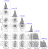 |
Fig. H.1 NS obtained posterior distributions for an atmosphere with T = 1500K and vrot=5210 m s−1, and for which we looked for HCN and C2H2. |
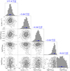 |
Fig. H.2 NS obtained posterior distributions for an atmosphere with T = 1500K and vrot = 5210 m s−1, and for which we looked for OH. |
References
- Amundsen, D. S., Baraffe, I., Tremblin, P., et al. 2014, A&A, 564, A59 [NASA ADS] [CrossRef] [EDP Sciences] [Google Scholar]
- Artigau, E. Doyon, R., Hernandez, O., et al. 2018, SPIE Conf. Ser., 10709, 107091P [NASA ADS] [Google Scholar]
- Asplund, M., Grevesse, N., Sauval, A. J., & Scott, P. 2009, ARA&A, 47, 481 [NASA ADS] [CrossRef] [Google Scholar]
- Azevedo Silva, T., Demangeon, O. D. S., Santos, N. C., et al. 2022, A&A, 666, L10 [NASA ADS] [CrossRef] [EDP Sciences] [Google Scholar]
- Baraffe, I., Chabrier, G., & Barman, T. 2010, Rep. Progr. Phys., 73, 016901 [CrossRef] [Google Scholar]
- Barber, R. J., Strange, J. K., Hill, C., et al. 2014, MNRAS, 437, 1828 [CrossRef] [Google Scholar]
- Bauer, F. F., Zechmeister, M., & Reiners, A. 2015, A&A, 581, A117 [NASA ADS] [CrossRef] [EDP Sciences] [Google Scholar]
- Bertaux, J. L., Lallement, R., Ferron, S., Boonne, C., & Bodichon, R. 2014, A&A, 564, A46 [NASA ADS] [CrossRef] [EDP Sciences] [Google Scholar]
- Boucher, A., Darveau-Bernier, A., Pelletier, S., et al. 2021, AJ, 162, 233 [NASA ADS] [CrossRef] [Google Scholar]
- Boucher, A., Lafreniére, D., Pelletier, S., et al. 2023, MNRAS, 522, 5062 [NASA ADS] [CrossRef] [Google Scholar]
- Brogi, M., & Line, M. R. 2019, AJ, 157, 114 [Google Scholar]
- Brogi, M., Giacobbe, P., Guilluy, G., et al. 2018, A&A, 615, A16 [NASA ADS] [CrossRef] [EDP Sciences] [Google Scholar]
- Buchner, J., Georgakakis, A., Nandra, K., et al. 2014, A&A, 564, A125 [NASA ADS] [CrossRef] [EDP Sciences] [Google Scholar]
- Caffau, E., Ludwig, H. G., Steffen, M., Freytag, B., & Bonifacio, P. 2011, Sol. Phys., 268, 255 [Google Scholar]
- Casasayas-Barris, N., Orell-Miquel, J., Stangret, M., et al. 2021, A&A, 654, A163 [NASA ADS] [CrossRef] [EDP Sciences] [Google Scholar]
- Cheverall, C. J., Madhusudhan, N., & Holmberg, M. 2023, MNRAS, 522, 661 [NASA ADS] [CrossRef] [Google Scholar]
- Chiavassa, A., & Brogi, M. 2019, A&A, 631, A100 [NASA ADS] [CrossRef] [EDP Sciences] [Google Scholar]
- Cook, N. J., Artigau, É., Doyon, R., et al. 2022, PASP, 134, 114509 [NASA ADS] [CrossRef] [Google Scholar]
- Debras, F., Klein, B., Donati, J.-F., et al. 2024, MNRAS, 527, 566 [Google Scholar]
- Deibert, E. K., de Mooij, E. J. W., Jayawardhana, R., et al. 2021, AJ, 161, 209 [NASA ADS] [CrossRef] [Google Scholar]
- Deibert, E. K., de Mooij, E. J. W., Jayawardhana, R., et al. 2023, AJ, 166, 141 [NASA ADS] [CrossRef] [Google Scholar]
- Donati, J. F., Kouach, D., Moutou, C., et al. 2020, MNRAS, 498, 5684 [Google Scholar]
- Drummond, B., Carter, A. L., Hébrard, E., et al. 2019, MNRAS, 486, 1123 [NASA ADS] [CrossRef] [Google Scholar]
- Edwards, B., Changeat, Q., Baeyens, R., et al. 2020, AJ, 160, 8 [Google Scholar]
- Edwards, B., Changeat, Q., Tsiaras, A., et al. 2023, ApJS, 269, 31 [NASA ADS] [CrossRef] [Google Scholar]
- Ehrenreich, D., Lovis, C., Allart, R., et al. 2020, Nature, 580, 597 [Google Scholar]
- Fisher, C., & Heng, K. 2018, MNRAS, 481, 4698 [Google Scholar]
- Flowers, E., Brogi, M., Rauscher, E., Kempton, E. M. R., & Chiavassa, A. 2019, AJ, 157, 209 [Google Scholar]
- Foreman-Mackey, D., Hogg, D. W., Lang, D., & Goodman, J. 2013, PASP, 125, 306 [Google Scholar]
- Fu, G., Deming, D., Lothringer, J., et al. 2021, AJ, 162, 108 [NASA ADS] [CrossRef] [Google Scholar]
- Gandhi, S., Kesseli, A., Snellen, I., et al. 2022, MNRAS, 515, 749 [NASA ADS] [CrossRef] [Google Scholar]
- Gandhi, S., Kesseli, A., Zhang, Y., et al. 2023, AJ, 165, 242 [NASA ADS] [CrossRef] [Google Scholar]
- Gibson, N. P., Merritt, S., Nugroho, S. K., et al. 2020, MNRAS, 493, 2215 [Google Scholar]
- Gibson, N. P., Nugroho, S. K., Lothringer, J., Maguire, C., & Sing, D. K. 2022, MNRAS, 512, 4618 [NASA ADS] [CrossRef] [Google Scholar]
- Guillot, T., Fletcher, L. N., Helled, R., et al. 2023, ASP Conf. Ser., 534, eds. S. Inutsuka, Y. Aikawa, T. Muto, K. Tomida, & M. Tamura, 947 [Google Scholar]
- Harris, G. J., Tennyson, J., Kaminsky, B. M., Pavlenko, Y. V., & Jones, H. R. A. 2006, MNRAS, 367, 400 [Google Scholar]
- Hobson, M. J., Bouchy, F., Cook, N. J., et al. 2021, A&A, 648, A48 [NASA ADS] [CrossRef] [EDP Sciences] [Google Scholar]
- Horne, K. 1986, PASP, 98, 609 [Google Scholar]
- JWST Transiting Exoplanet Community Early Release Science Team (Ahrer, E.-M., et al.) 2023, Nature, 614, 649 [NASA ADS] [CrossRef] [Google Scholar]
- Kawauchi, K., Narita, N., Sato, B., & Kawashima, Y. 2022, PASJ, 74, 225 [CrossRef] [Google Scholar]
- Kesseli, A. Y., & Snellen, I. A. G. 2021, ApJ, 908, L17 [Google Scholar]
- Kesseli, A. Y., Snellen, I. A. G., Casasayas-Barris, N., Mollière, P., & Sánchez-López, A. 2022, AJ, 163, 107 [NASA ADS] [CrossRef] [Google Scholar]
- Klein, B., Debras, F., Donati, J.-F., et al. 2024, MNRAS, 527, 544 [Google Scholar]
- Kokori, A., Tsiaras, A., Edwards, B., et al. 2022, ApJS, 258, 40 [NASA ADS] [CrossRef] [Google Scholar]
- Kurucz, R. L. 1993, SYNTHE spectrum synthesis programs and line data (Cambridge, Mass.: Smithsonian Astrophysical Observatory) [Google Scholar]
- Landman, R., Sánchez-López, A., Mollière, P., et al. 2021, A&A, 656, A119 [NASA ADS] [CrossRef] [EDP Sciences] [Google Scholar]
- Line, M. R., Wolf, A. S., Zhang, X., et al. 2013, ApJ, 775, 137 [NASA ADS] [CrossRef] [Google Scholar]
- Line, M. R., Brogi, M., Bean, J. L., et al. 2021, Nature, 598, 580 [NASA ADS] [CrossRef] [Google Scholar]
- Madhusudhan, N., Bitsch, B., Johansen, A., & Eriksson, L. 2017, MNRAS, 469, 4102 [NASA ADS] [CrossRef] [Google Scholar]
- Mansfield, M., Line, M., Bean, J., et al. 2022, BAAS, 54, 102.112 [NASA ADS] [Google Scholar]
- Mollière, P., Wardenier, J. P., van Boekel, R., et al. 2019, A&A, 627, A67 [Google Scholar]
- Mollière, P., Stolker, T., Lacour, S., et al. 2020, A&A, 640, A131 [Google Scholar]
- Pelletier, S., Benneke, B., Darveau-Bernier, A., et al. 2021, AJ, 162, 73 [NASA ADS] [CrossRef] [Google Scholar]
- Pelletier, S., Benneke, B., Ali-Dib, M., et al. 2023, Nature, 619, 491 [NASA ADS] [CrossRef] [Google Scholar]
- Pluriel, W. 2023, Remote Sens., 15, 635 [NASA ADS] [CrossRef] [Google Scholar]
- Polyansky, O. L., Kyuberis, A. A., Zobov, N. F., et al. 2018, MNRAS, 480, 2597 [NASA ADS] [CrossRef] [Google Scholar]
- Rothman, L. S., Gordon, I. E., Barber, R. J., et al. 2010, J. Quant. Spec. Radiat. Transf., 111, 2139 [NASA ADS] [CrossRef] [Google Scholar]
- Rothman, L. S., Gordon, I. E., Babikov, Y., et al. 2013, J. Quant. Spec. Radiat. Transf., 130, 4 [NASA ADS] [CrossRef] [Google Scholar]
- Sánchez-López, A., Landman, R., Mollière, P., et al. 2022, A&A, 661, A78 [NASA ADS] [CrossRef] [EDP Sciences] [Google Scholar]
- Savel, A. B., Kempton, E. M. R., Malik, M., et al. 2022, ApJ, 926, 85 [NASA ADS] [CrossRef] [Google Scholar]
- Seidel, J. V., Ehrenreich, D., Wyttenbach, A., et al. 2019, A&A, 623, A166 [NASA ADS] [CrossRef] [EDP Sciences] [Google Scholar]
- Snellen, I. A. G., de Kok, R. J., de Mooij, E. J. W., & Albrecht, S. 2010, Nature, 465, 1049 [Google Scholar]
- Soubiran, C., Jasniewicz, G., Chemin, L., et al. 2018, A&A, 616, A7 [NASA ADS] [CrossRef] [EDP Sciences] [Google Scholar]
- Tabernero, H. M., Zapatero Osorio, M. R., Allart, R., et al. 2021, A&A, 646, A158 [NASA ADS] [CrossRef] [EDP Sciences] [Google Scholar]
- Taylor, J., Radica, M., Welbanks, L., et al. 2023, MNRAS, 524, 817 [NASA ADS] [CrossRef] [Google Scholar]
- Tremblin, P., Amundsen, D. S., Mourier, P., et al. 2015, ApJ, 804, L17 [CrossRef] [Google Scholar]
- Tsiaras, A., Waldmann, I. P., Zingales, T., et al. 2018, AJ, 155, 156 [NASA ADS] [CrossRef] [Google Scholar]
- von Essen, C., Mallonn, M., Hermansen, S., et al. 2020, A&A, 637, A76 [NASA ADS] [CrossRef] [EDP Sciences] [Google Scholar]
- Wardenier, J. P., Parmentier, V., Lee, E. K. H., Line, M. R., & Gharib-Nezhad, E. 2021, MNRAS, 506, 1258 [NASA ADS] [CrossRef] [Google Scholar]
- Wardenier, J. P., Parmentier, V., Line, M. R., & Lee, E. K. H. 2023, MNRAS, 525, 4942 [NASA ADS] [CrossRef] [Google Scholar]
- West, R. G., Hellier, C., Almenara, J. M., et al. 2016, A&A, 585, A126 [NASA ADS] [CrossRef] [EDP Sciences] [Google Scholar]
- Yan, F., Nortmann, L., Reiners, A., et al. 2023, A&A, 672, A107 [NASA ADS] [CrossRef] [EDP Sciences] [Google Scholar]
- Žák, J., Kabáth, P., Boffin, H. M. J., Ivanov, V. D., & Skarka, M. 2019, AJ, 158, 120 [Google Scholar]
According to http://research.iac.es/proyecto/exoatmospheres/index.php, a database referencing exoplanet atmosphere studies.
All Tables
Priors used in our nested sampling algorithm through this paper, and posteriors found in Sects. 4.1 (Post. 1), 4.2 (Post. 2), 4.3 (Post. 3), 4.4 (Post. 4), and 5.1.2 (Post. 5).
Kp and V0 values for maximum S/N position obtained for water detection in each transit half.
List of chemical species reported as detected (green), tentatively detected (orange), or not detected (red) in previous publications and this work. For each species has been indicated the instrument used and the corresponding reference for the study of its presence in the atmosphere. Empty cells indicate that the species has not been explicitly included in a published study with the corresponding instrument.
All Figures
|
Fig. 1 Continuum-normalised light-curve, air mass, radial velocity (RV) correction (containing RV contributions of the barycentric Earth motion and the stellar systemic velocity), and peak S/N per velocity bin over the course of the transit of WASP-76 b as a function of the orbital phase (from top to bottom), computed using the parameters listed in Table 1. The grey band indicates the transit duration of the planet, from first to fourth contact. The horizontal dashed line in the bottom panel represents the average value of the peak S/N. |
| In the text | |
|
Fig. 2 Map resulting from cross-correlation between reduced data of WASP-76 b and spectra from a model containing H2O opacity lines. The S/N varies from -3.86 to 7.29, with the maximum peak in S/N of 7.29 obtained for Kp = 180 km s−1 and V0 = −6.0 km s−1. The black lines (full, dashed and dotted), respectively, represent the 1, 2, and 3 σ contours. The white dashed lines represent the theoretical values from Ehrenreich et al. (2020) of Kp = 196.52 km s−1 and V0 = −5.3 km s−1. |
| In the text | |
|
Fig. 3 Same as Fig. 2, but using models containing only CO. The S/N varies from -3.30 to 5.03. The maximum S/N was obtained for Kp = 200 km s−1 and V0 = −11.5 km s−1. |
| In the text | |
|
Fig. 4 Temperature profile from extended data Fig. 5 in Pelletier et al. (2023) (blue) compared to the isothermal temperature profile from Fig. 7 in Edwards et al. (2020) (green) and the isothermal temperature profile retrieved in Fig. E.1 with T = 1355 K (red), with the shaded regions representing the 1 and 3σ error bars (only 1σ represented for the profile from Edwards et al. 2020). |
| In the text | |
|
Fig. 5 Representation of possible C/O and [(C+O)/H] values for the posteriors of log(H2O) and log(CO). The white lines (full, dashed, and dotted), respectively, represent the 1, 2, and 3σ contours shown in Fig. E.1. For the whole range of possible values of log(H2O)MMR and log(CO)MMR, we calculated the corresponding values of the C/O and [(C + O)/H] ratios. The background represents the resulting values of C/O ratio. The coloured lines indicate the values of [(C+O)/H]. |
| In the text | |
|
Fig. 6 Variations in VMR of H2O and CO depending on pressure calculated by ATMO for C/O = 0.5, 1,1.6, and 2 × solar. |
| In the text | |
|
Fig. 7 Mean abundances in VMR of C2H2 and HCN (averaged over pressures from 100 to 10−4 bar). The black dashed lines correspond to the upper limit abundances found by the data simulator of log(C2H2)MMR = −6 and log(HCN)MMR = −4. |
| In the text | |
|
Fig. 8 Mean abundances in VMR of OH (averaged over pressures from 100 to 10−4 bar) as a function of the corresponding C/O ratio as estimated using Eq. (5). The black dashed line corresponds to the upper limit abundance found by the data simulator of log(OH)MMR= −4. |
| In the text | |
|
Fig. 9 Scatter plot showing relative amplitude difference as function of radial velocity difference between the first and second half of the transit from Kesseli et al. (2022), to which we added our results for H2O. |
| In the text | |
|
Fig. 10 Comparison between cross-correlation profiles for different scenarios for H2O obtained in Wardenier et al. (2023) and radial velocities we obtained for H2O from the mean cross-correlation functions for each half of transit. The ‘nominal’ profile (green) was obtained for a weak-drag model, the ‘cold morning limb’ profile (red) for a model for which the temperature was reduced on the leading limb, the ‘optically thick clouds’ profile (blue) for adding clouds as in Savel et al. (2022), and the ‘no TiO/VO’ profile (purple) for removing TiO and VO from the GCM calculations, considering them cold-trapped. The black dots correspond to the radial velocities obtained from Gaussian fits to the mean cross-correlation functions for each half of transit, the horizontal black bars corresponding to the associated errors, and the vertical black bars indicate the associated phase range. The grey band indicates the transit duration from post-ingress to pre-egress. |
| In the text | |
|
Fig. B.1 Cross-correlation trails for H2O (top) and CO (bottom). The dashed lines correspond to the absorption trails indicated for each species by the Kp and V0 values reported in Section 4.1. The black dotted lines correspond to the ’kinked’ absorption trail reported for Fe. The grey dotted horizontal lines correspond to the beginning and end of the transit. |
| In the text | |
|
Fig. C.1 Distribution of log(C/O), with the top panel representing the priors and the bottom panel the posteriors. The blue lines correspond to when using uniform priors for the distributions of the MMRs of H2O and CO. The orange lines correspond to when using a uniform linear distribution of the C/O ratio. The green lines correspond to using a uniform distribution in log space of the C/O ratio. |
| In the text | |
|
Fig. D.1 Map resulting from cross-correlation between reduced data of WASP-76 b from the first half of the transit and spectra from a model containing H2O opacity lines (log(H2O)MMR = −5.0), with T = 1500 K. The S/N varies from −3.16 to 4.65, with the maximum S/N of 4.65 obtained for Kp = 184 km s−1 and V0 = −4.5 km s−1. |
| In the text | |
|
Fig. D.2 Map resulting from cross-correlation between reduced data of WASP-76 b from the second half of the transit and spectra from a model containing H2O opacity lines (log(H2O)MMR = −5.0), with T = 1500 K. The S/N varies from −3.39 to 4.75, with the maximum S/N of 4.75 obtained for Kp =216 km s−1 and V0 =−11.5 km s−1. |
| In the text | |
|
Fig. E.1 Corner plot showing NS results of our retrieval using WASP-76 b data. The black lines (full, dashed, and dotted) represent the 1, 2, and 3 sigma contours, respectively. The maximum probability and 1σ values found are represented for each histogram on the diagonal by the blue dot and bar. |
| In the text | |
|
Fig. F.1 Posterior distributions obtained from NS algorithm using cloud-free models with T = 1500K. Represented by the red dashed line is the expected rotation velocity for WASP-76 b (see Section 4.4). |
| In the text | |
|
Fig. G.1 NS posterior distribution for using C/O and [(C+O)/H] as priors. The red dashed lines represent the values found in Figure E.1. |
| In the text | |
|
Fig. H.1 NS obtained posterior distributions for an atmosphere with T = 1500K and vrot=5210 m s−1, and for which we looked for HCN and C2H2. |
| In the text | |
|
Fig. H.2 NS obtained posterior distributions for an atmosphere with T = 1500K and vrot = 5210 m s−1, and for which we looked for OH. |
| In the text | |
Current usage metrics show cumulative count of Article Views (full-text article views including HTML views, PDF and ePub downloads, according to the available data) and Abstracts Views on Vision4Press platform.
Data correspond to usage on the plateform after 2015. The current usage metrics is available 48-96 hours after online publication and is updated daily on week days.
Initial download of the metrics may take a while.