| Issue |
A&A
Volume 698, June 2025
|
|
|---|---|---|
| Article Number | A268 | |
| Number of page(s) | 22 | |
| Section | Extragalactic astronomy | |
| DOI | https://doi.org/10.1051/0004-6361/202452926 | |
| Published online | 19 June 2025 | |
Multi-wavelength properties of z ≳ 6 Laser Interferometer Space Antenna detectable events
1
Scuola Normale Superiore, Piazza dei Cavalieri 7, 56126
Pisa, PI, Italy
2
Dipartimento di Fisica, Sapienza, Università di Roma, Piazzale Aldo Moro 5, 00185
Roma, Italy
3
Dipartimento di Fisica dell’Università di Trieste, Sez. di Astronomia, Via Tiepolo 11, I-34131
Trieste, Italy
4
INAF, Osservatorio Astronomico di Trieste, Via Tiepolo 11, I-34131
Trieste, Italy
5
INFN, Instituto Nazionale di Fisica Nucleare, Via Valerio 2, I-34127
Trieste, Italy
6
ICSC – Italian Research Center on High Performance Computing, Big Data and Quantum Computing, Via Magnanelli 2, 40033
Casalecchio di Reno, Italy
7
INAF – Osservatorio Astronomico di Bologna, Via Piero Gobetti 93/3, I-40129
Bologna, Italy
⋆ Corresponding author: srija.chakraborty@sns.it
Received:
8
November
2024
Accepted:
22
March
2025
We investigated the intrinsic and observational properties of z ≳ 6 galaxies that host the coalescence of massive black holes (MBHs; MBH ∼ 105−6 M⊙) giving rise to gravitational waves (GWs) detectable with the Laser Interferometer Space Antenna (LISA). We adopted a zoom-in cosmological hydrodynamical simulation of galaxy formation and black hole (BH) co-evolution, based on the GADGET-3 code, zoomed-in on an Mh ∼ 1012 M⊙ dark matter halo at z = 6, which hosts a fast accreting (Ṁ ∼ 35 M⊙ yr−1) super-massive black hole (SMBH; MBH ∼ 109 M⊙) and a star-forming galaxy (SFR ∼ 100 M⊙ yr−1). Tracing the SMBH’s formation backwards in time, we identified the merger events associated with its formation and selected those that are detectable with LISA. Among these LISA-detectable events (LDEs), we selected those–based on their intrinsic properties (Ṁ, SFR, gas metallicity, and dust mass)–that were expected to be bright in one or more electromagnetic (EM) bands, such as rest-frame X-ray, UV and far-infrared (FIR). After considering the effect of delay due to dynamical friction in the MBH coalescence, we further restricted our selection to those LDEs that are still occurring at z ≳ 6. We find that ∼20–30% of the LDEs and their host galaxies are also detectable with EM telescopes. We post-processed these events with dust radiative transfer calculations to make accurate predictions about their spectral energy distributions (SEDs) and continuum maps in the JWST to ALMA wavelength range. We compared the spectra arising from galaxies hosting the merging MBHs with those arising from the active galactic nuclei (AGN) powered by single accreting BHs. We find that identifying an LDE from the continuum SEDs is impossible because of the absence of specific imprints from the merging MBHs. Finally, we computed the profile of the Hα line arising from LDEs, taking into account both the contribution from their star-forming regions and the accreting MBHs. We find that the presence of two accreting MBHs would be difficult to infer even if both MBHs accrete at super-Eddington rates (λEDD ∼ 5 − 10). We conclude that the combined detection of GW and EM signals from z ≳ 6 MBHs is challenging (if not impossible) not only because of the poor sky-localization (∼10 deg2) provided by LISA, but also because the loudest GW emitters (MBH ∼ 105−6 M⊙) are not massive enough to leave significant signatures (e.g. extended wings) in the emission lines arising from the broad line region.
Key words: gravitational waves / galaxies: high-redshift / quasars: supermassive black holes
© The Authors 2025
 Open Access article, published by EDP Sciences, under the terms of the Creative Commons Attribution License (https://creativecommons.org/licenses/by/4.0), which permits unrestricted use, distribution, and reproduction in any medium, provided the original work is properly cited.
This article is published in open access under the Subscribe to Open model. Subscribe to A&A to support open access publication.
1. Introduction
Follow-up observations of z ∼ 6 − 7.5 quasars–the brightest (with bolometric luminosities Lbol ≳ 1046 erg s−1) and the most distant active galactic nuclei (AGN) discovered so far–show us that these sources are powered by super-massive black holes (SMBHs) (SMBHs, 108−1010 M⊙, see a recent review by Fan et al. 2023, and references therein). The existence of these SMBHs challenges theoretical models of black hole (BH) formation and evolution that strive to understand both the origin and mass of SMBH seeds, and their ability to grow fast enough to assemble SMBHs in less than 1 Gyr (the age of the Universe at z ≳ 6; e.g. Volonteri et al. 2003; Latif & Ferrara 2016; Valiante et al. 2017; Volonteri et al. 2021).
The most recent James Webb Space Telescope (JWST) data has revealed the presence of accreting massive black holes (MBHs; 106−108 M⊙) in galaxies up to z ∼ 10 − 11 (e.g. Bosman et al. 2023; Greene et al. 2024; Goulding et al. 2023; Furtak et al. 2024; Kokorev et al. 2023; Larson et al. 2023; Maiolino 2024a; Kovács et al. 2024), providing an unprecedented testing ground for theoretical models (e.g. Jeon et al. 2025; Trinca et al. 2023; Pacucci et al. 2023; Schneider et al. 2023; Bhatt et al. 2024). In particular, JWST data has revealed the presence of dual AGN at z ∼ 6 − 7 (Übler et al. 2024; Matsuoka et al. 2024), powered by pairs of accreting MBHs. Since dual AGN are considered the precursors of merging MBHs (Saeedzadeh et al. 2024), these findings have been interpreted as evidence that MBH mergers are common in the distant Universe. On the one hand, the existence of MBH merging is expected from theoretical models; on the other hand, the actual number of MBH mergers depends on several properties of the MBHs and their host galaxies.
According to the hierarchical structure formation paradigm, large galaxies are assembled through the merging of smaller galaxies (Press & Schechter 1974). Since MBHs are nested in the nuclei of their host galaxies (Lynden-Bell 1969; Wise et al. 2019), galaxy mergers can lead to the formation of MBH pairs (Yu & Tremaine 2002; Volonteri et al. 2021).
Depending on the mass ratio of the MBH pair, on the initial separation between the MBHs, and on the physical properties of their host galaxies, the dynamical friction exerted by the surrounding gas and stars on the MBHs (e.g. Begelman et al. 1980; Armitage & Natarajan 2002; Sesana & Khan 2015) may reduce their initial separation and modify their dynamics (see the recent paper by Damiano et al. 2024, and references therein), eventually leading to their coalescence and the subsequent emission of gravitational waves (GWs).
The European Space Agency’s Science Programme Committee has recently acknowledged the challenge of detecting and studying GWs from space with the approval of the Laser Interferometer Space Antenna (LISA) mission. Given its sensitivity and frequency coverage (10−4 − 10−1 Hz), LISA is expected to detect GWs from various low frequency sources, including GWs arising from MBH (104−107 M⊙) mergers at high redshift (z ∼ 6 − 10) (Amaro-Seoane et al. 2023), similarly to what is anticipated for proposed missions such as TianQin (Luo et al. 2016) and Taiji (Ruan et al. 2020). The thrilling results obtained by the NANOGrav Pulsar Timing Array (PTA), the Parkes PTA (Manchester et al. 2013), the International PTA (Verbiest et al. 2016; Antoniadis et al. 2022), the Indian PTA (Tarafdar et al. 2022), the Chinese PTA (Xu et al. 2023), and the European PTA (EPTA Collaboration, InPTA Collaboratio 2023; Agazie et al. 2023)–all of which have found a 3σ evidence for a stochastic GW background likely originating from the mergers of MBHs–encourage further studies of merging MBHs.
Furthermore, the joint detection of GWs and electromagnetic (EM) signals from the host galaxies of the merging MBHs provide several exciting opportunities: i) to obtain independent constraints on cosmological parameters by comparing the luminosity distance directly observable by GWs with the redshift inferred from the EM emission (e.g. Schutz 1986; Abbott et al. 2018); ii) to study BH binaries properties (e.g. masses, orbital parameters, and Eddington ratios) and characterise their environment (e.g. Bogdanović et al. 2022); and iii) to clarify open issues related to the formation of SMBHs at high redshift (z ≳ 6; e.g. Sesana et al. 2004; Lops et al. 2023). Nevertheless, the detection of EM signatures from LISA detectable events (LDEs) is extremely challenging because of the poor sky-localization (∼10 deg2) provided by LISA (e.g. Mangiagli et al. 2020; Lops et al. 2023; Chakraborty et al. 2023). For these reasons, any hint about the properties of the host galaxies hosting LDEs is strikingly useful.
The detectability of EM signatures from LDEs has been investigated both through semi-analytical models and numerical simulations. For z ≲ 3, Izquierdo-Villalba et al. (2023) used a semi-analytical model to explore host galaxy properties of LISA MBHs at this redshift range and showed that the hosts display properties of optically dim, gas-rich, star-forming, disc-dominated, low mass galaxies. However, it is challenging to distinguish a LISA host galaxy from galaxies hosting singular BHs with similar mass. Valiante et al. (2021) adopted the GAMETE semi-analytical model and found that mergers involving heavy seeds (∼ 105−107 M⊙) are detectable by Athena (JWST) up to z ∼ 16 (z ∼ 13). Using a semi-analytical galaxy formation and evolution model, Mangiagli et al. (2022) showed that LDEs are expected to be associated with faint EM emission, which challenges the observational capabilities of future telescopes and may provide only a few (∼7 − 20) multi-messenger detection of merging MBHs. The analysis of the OBELISK simulations (Dong-Páez et al. 2023) suggests that at z > 3.5 the signal arising from merging BHs is fainter than their star-forming host galaxies and this is hardly detectable in the rest frame UV. Conversely, 5–15% of the merging BHs analysed exhibit X-ray emission that is sufficiently bright to be detected with sensitive X-ray instruments. Numerical simulations have been also used to investigate whether morphological (e.g. DeGraf et al. 2021; Bardati et al. 2024) and/or spectral signatures (Bardati et al. 2024) are associated with MBH mergers. These studies found that it is possible to statistically identify their host galaxies, with an accuracy increasing with chirp mass and the mass ratio.
In this study, we explored the results presented in Chakraborty et al. (2023, hereafter C23), which were based on the zoom-in cosmological hydro-dynamical simulations developed by Valentini et al. (2021, hereafter V21). Here, we focused on MBH pairs that, according to simulation prescriptions, were expected to merge at z ≳ 6. We then carried out the following steps: (i) We characterised their intrinsic properties (e.g. the star formation rate (SFR) of the host galaxy and the accretion rates of the MBHs); (ii) We computed their observable properties (e.g. the UV, the far-infrared or FIR, and the X-ray emissions); and (iii) We checked whether they were detectable with current and upcoming EM telescopes (e.g. ALMA, JWST, Chandra, and Lynx). In particular, with regards to (ii), we post-processed the hydrodynamical simulations with radiative transfer calculations by exploiting the SKIRT code. The paper is organised as follows: in Sect. 2, we present the simulations adopted and post-processed with radiative transfer calculations; in Sect. 3, we select the LDEs that are the most promising for a possible EM detection; in Sect. 4, we present our results, including the outcomes of RT simulations; in Sect. 5, we compute the shape of the Hα line from MBH pairs; and finally in Sect. 6, we summarise and discuss the main results of our work.
2. Numerical models
In this section, we describe the main properties of the cosmological hydrodynamical simulations analysed in this work as well as the radiative transfer code implemented in post-processing. We select the AGN_fid run of the suite presented by V21 and previously analysed by C23 to compute the GW properties of the merging MBHs predicted by simulations.
2.1. Hydrodynamical simulations
The simulations were performed with the TreePM (particle mesh) + SPH (Smoothed Particles Hydrodynamics) code GADGET-3, an evolution of the public GADGET-2 code (Springel 2005). They follow the evolution of a halo whose mass is ∼1012 M⊙ at z = 6. In particular, we considered the AGN_fid run from V21, featuring star formation, stellar feedback, and thermal AGN feedback, among other physical processes. We summarise in the following sections the main features of the simulations that are relevant to the present study, while referring to the papers above for details.
2.1.1. Initial conditions and resolution
The code MUSIC1 (Hahn & Abel 2011) was used to generate the initial conditions of this simulation2. First, a dark matter (DM)-only simulation was run from z = 100 to z = 6, with the DM particles having a mass of 9.4 × 10⁸ M⊙ in a co-moving volume of (148 Mpc)3. A halo as massive as Mhalo = 1.12 × 10¹² M⊙ at z = 6 was selected for the zoom-in, full-physics simulation, where the highest resolution particles have a mass MDM = 1.55 × 10⁶ M⊙ and Mgas = 2.89 × 10⁵ M⊙. The gravitational softening lengths employed were ϵDM = 0.72 ckpc3 and ϵbar = 0.41 ckpc for DM and baryon particles, respectively.
2.1.2. Sub-resolution physics
-
Cooling, star formation, and stellar feedback: A multiphase, sub-resolution model of the interstellar medium (ISM) described by the MUlti Phase Particle Integrator (MUPPI) (Murante et al. 2010, 2015; Valentini et al. 2017, 2018, 2019) was used. It features metal-line cooling, an H2-based star formation criterion, thermal and kinetic stellar feedback, a UV background, and a model for stellar chemical evolution (Tornatore et al. 2007).
-
Black holes seeding and merging: The BHs were treated as collisionless sink particles with a seed mass of MBH, seed = 1.48 × 10⁵ M⊙ seeded in DM halos when they first exceed a mass of MDM, seed = 1.48 × 10⁹ M⊙. This seeding prescription captures both the results of the so-called direct collapse BH scenario–which predicts SMBH seeds of mass MBH, seed ∼ 104 − 106 M⊙ (Ferrara et al. 2014; Haehnelt & Rees 1993; Mayer & Bonoli 2019)–and the recent prescription proposed by Ziparo et al. (2025) based on primordial BHs (see, e.g., a recent review by Carr & Green 2025). Two BHs merge when the following conditions are met: (i) their relative distance is less than twice the BH gravitational softening length and (ii) their relative velocity is lower than the sound speed of the local ISM. The merger is instantaneous; that is, no time delays between binary formation and coalescence are considered. The final BH resulting from the collision occupies the position of the more massive BH, which underwent the merger. BH repositioning or ’pinning’ is also implemented to prevent BHs from wandering from the centre of the halo in which they reside: at each time-step, BHs are shifted towards the position of minimum gravitational potential within their softening length instantaneously (as also done in e.g. Booth & Schaye 2009; Schaye et al. 2015; Weinberger et al. 2017; Pillepich et al. 2018).
-
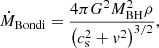
BH accretion: Along with BH-BH mergers, BHs can also grow via gas accretion from their surroundings. Gas accretion is described by the classical Bondi-Hoyle-Lyttleton accretion solution (Hoyle & Lyttleton 1939; Bondi & Hoyle 1944; Bondi 1952; Edgar 2004) given by
where G is the gravitational constant, ρ is the gas density, cs is its sound speed, and v is the velocity of the BH relative to the gas. These quantities are evaluated by averaging the SPH gas particles within the BH smoothing length with kernel-weighted contributions. Equation (1) is used to estimate the contribution to the accretion rate from the cold and hot phase of the ISM separately (Steinborn et al. 2015; Valentini et al. 2020). Accretion from the cold gas is reduced by taking into account its angular momentum (see Valentini et al. 2020, for details). The BH accretion rate is capped to the Eddington accretion rate.
-
AGN feedback: A fraction of the accreted rest-mass energy is radiated away with a radiative efficiency ϵr, thereby providing a bolometric luminosity for a BH given by
where c is the speed of light and ϵr = 0.034. A fraction ϵf = 10−4 (V21) of the radiated luminosity Lbol is coupled thermally and isotropically to the gas surrounding the BH. This AGN feedback energy is distributed to both the hot and cold phases of the multiphase gas particles within the BH smoothing volume (Valentini et al. 2020).
2.2. Galaxy-merging MBHs association
From the cosmological hydrodynamical simulations, we identified merger events as described in C23. To associate a host galaxy with a merger event, we followed the procedure described in Zana et al. (2022) (see also Sect. 4.1 in C23). We assigned each merger event to the galaxy whose centre of mass is closest to the position of the most massive BH. Hereafter, we refer to the most massive BH as the “primary BH” (BHp) and to the least massive as the “secondary BH” (BHs).
As mentioned in Sect. 2.1.2, in the V21 simulations, the merger between two MBHs occurs instantaneously. However, the actual coalescence of two MBHs depends on their interaction with gas and stars in their surroundings which in turn allows them to lose energy and spiral inwards gradually (Chandrasekhar 1943; Ostriker 1999). This process delays the MBH merger with respect to what is assumed in the adopted simulations. As in C23, we applied a post-processing correction to the coalescing time of MBH mergers by including a time delay due to dynamical friction from the surrounding stars. In this case, the dynamical friction timescale was computed as (Krolik et al. 2019; Volonteri et al. 2020)
Here, a is the distance of the BHp5 from the galaxy centre; σ is the stellar velocity dispersion; and Λ is given by

where M* and MBHs denote the stellar mass of the host galaxy and the mass of the BHs, respectively.
2.3. Radiative transfer calculations
We performed radiative transfer (RT) calculations including dust with the code SKIRT6, a Monte Carlo radiative transfer solver designed to model radiation fields in dusty media by accounting for dust grain scattering, absorption, and their ensuing re-emission in the IR (e.g. Baes et al. 2003; Camps & Baes 2015). We used a similar numerical setup to the one in Di Mascia et al. 2021 summarised below.
For the RT calculations, we selected a cubic region with a side length of 40 kpc, centred on the centre of mass of the most-massive halo, where the galaxies associated with the merger events reside. This region was then post-processed in SKIRT by using a computational box of the same size. The RT simulation requires two main ingredients: a source component (e.g. stars and AGN), which determines the radiation field before accounting for dust attenuation; and a dust component, which absorbs and scatters the radiation, and then thermally re-emits photons, altering the radiation field. We describe how these two components are imported from the hydrodynamic simulation in SKIRT in the following subsections.
2.3.1. Dust properties
Dust is distributed in the SKIRT computational domain by assuming a linear scaling with gas metallicity7 (e.g. Draine et al. 2007) according to a ‘dust-to-metal ratio’ fd that quantifies the mass fraction of metals locked into dust given by
where Mdust is the dust mass and MZ is the total mass of all the metals in each gas particle in the hydrodynamical simulation. Gas particles hotter than 106 K are assumed to be dust-free because of thermal sputtering (e.g. Draine & Salpeter 1979). We adopted the value of fd = 0.1, which is consistent with RT simulations reproducing the emission of high-redshift galaxies (e.g. Behrens et al. 2018).
The dust distribution derived from the gas particles is then distributed into a dust grid in SKIRT. We adopted an octree grid with nine levels of refinement, corresponding to a maximum spatial resolution of ≈80 pc, comparable to that of the hydrodynamical simulations at the redshifts of the events. Using the results of Weingartner & Draine 2001, we assumed a dust composition that reproduces the extinction curve of the Small Magellanic Cloud (SMC). We considered dust self-absorption in our calculations but neglected non-local thermal equilibrium (NLTE) corrections to dust emission. We did not include heating from cosmic microwave background (CMB) radiation.
2.3.2. Stellar and AGN radiation
Stellar and BH particles were treated as point sources of radiation. We described stellar emission by using the family of stellar synthesis models in Bruzual & Charlot 2003. For the BHs, we adopted the AGN fiducial spectral energy distribution (SED) introduced in Di Mascia et al. 2021, which can be written as a composite power law given by
where i refers to the bands in which we decomposed the spectra. The coefficients ci are determined by imposing the continuity of the function based on the slopes αi (see Table 2 in Di Mascia et al. 2021, for specific values of the coefficients). The SED was then normalised according to the bolometric luminosity of the BH, as expressed by Eq. (2).
The radiation field was sampled using a grid composed of 200 logarithmically spaced bins, covering the rest-frame wavelength range [0.1 − 103] μm. A total of 106 photon packets per wavelength bin was launched from each source8.
 |
Fig. 1. The PDFs of different intrinsic properties of LDEs associated with a host galaxy before (purple dashed line) and after (black solid line) adding time delay due to DF at z > 6. In each panel, the lavender bars represent the LDEs, which are also EMDEs for all events (see Sect. 3.2), while the red region represents the same for the events that occur after accounting for time delays due to DF. In the top panel from left to right, respectively: Chirp mass of LISA events, stellar mass, SFRs, and sSFRs of the host galaxies. In the bottom panel from left to right, respectively: total accretion rates of LISA events, gas mass, metallicity, and dust mass of the host galaxies. Mass and metallicities are represented in solar units. |
3. Selection of LDEs for RT calculations
Among the GW events previously identified in C23, we select in this section those LDEs that are both detectable with LISA and with EM follow-up observations (i.e. EM detectable Events or EMDEs). For LDEs, we computed the signal-to-noise ratio (S/N) of the GW emission from merging MBHs and selected those events that are characterised by S/N > 5 (see Sect. 5.1 in C23). To briefly summarise, in C23, we calculated the S/N of merging MBHBs over a given observational time τ using the equation
![$$ \begin{aligned} \left(\frac{S}{N}\right)_{\Delta f}^2= \int _{f}^{f+\Delta f} d\ln f\prime \, \left[ \frac{h_c(f\prime _r)}{h_{\rm rms}(f\prime )} \right]^2 \end{aligned} $$](/articles/aa/full_html/2025/06/aa52926-24/aa52926-24-eq7.gif)
from Flanagan & Hughes (1998), where fr is the GW rest-frame frequency, f = fr/(1 + z) is the observed frequency, and Δf is the frequency shift in the duration of τ. Here, hc is the characteristic strain, defined as the sky- and polarisation-averaged strain amplitude accumulated over the number of cycles spent by MBHBs in the LISA bandwidth. The quantity hrms denotes the effective rms noise of the instrument. Recalling that LISA is sensitive at frequencies [10−4–1.0] Hz, we note that a merger event can only be detected when the emitted GWs enter the LISA frequency range (even though the MBHB might still emit GWs outside this frequency window). The S/N corresponding to this minimum frequency limit is denoted as S/Nthresh, which we set to 5 in order for a GW event to be detected by LISA.
3.1. Intrinsic properties of systems hosting merging MBHs
Following the procedure described in Sect. 2.2, we first associated each GW event previously identified in C23 with the intrinsic properties of the galaxies hosting merging MBHs: that is, the total (primary plus secondary) BH accretion rate (BHAR), the star formation rate, the specific star formation rate (sSFR), the metallicity (Z), the dust mass (Mdust), the stellar mass (Mstellar), and the gas mass (Mgas). We also show the chirp mass distribution of the merging MBHs in the same figure. In Table B.1, we report the intrinsic properties of the merger events with which a galaxy is associated without including dynamical friction (DF) effects. In what follows, we report the results with and without including DF effects.
In Fig. 1, we show the probability distribution function (PDF) of the intrinsic properties of all the LDEs assuming instantaneous merger (purple dashed line, Tot LDE). This PDF is normalised to one. For these events, we computed the time delay due to stellar DF (see Sect. 4.2 in C23). Taking into account time delay effects, we then selected only those MBHs whose merger occurred at z ≳ 6. The black solid line denotes the LDEs among these events, denoted as DF LDEs in the figure. For visual purposes, we normalise the PDFs to the fraction of LDEs that, after accounting for DF, still occur at z ≳ 6.
In the top left panel of Fig. 1, we show the chirp mass of LDEs before and after considering the DF effect. We find that the average chirp mass of the total LDEs is 1.3 × 10⁶ M⊙. When adding the DF time delay, the average chirp mass decreases to 1.1 × 10⁶ M⊙. The top second panel depicts the stellar mass distribution of the host galaxies. We find an average of Mstellar ∼ 4.8 × 10⁹ M⊙ (∼8.5 × 10⁸ M⊙) without (with) including the delays due to DF. The third (fourth) panel of the top row show the distribution of the SFR (specific SFR, denoted as sSFR) in the host galaxies of LDEs. We find that the average SFR (sSFR) of the LDEs in the AGN_fid is ∼ 29 M⊙ yr−1 (sSFR ∼ 7.2 Gyr−1), or ∼ 9 M⊙ yr−1 (∼ 9.3 Gyr−1) if DF effects are taken into account. From the bottom row of Fig. 1, the left panel shows that the total BHAR of LDEs in the AGN_fid runs peaks at Ṁ ∼ 0.01 M⊙ yr−1 and spans the range [∼ 10−6−30 M⊙ yr−1]. When considering the DF time delay effect, the highest BHAR of LDEs shifts to a lower value of approximately Ṁ ∼ 0.1 M⊙ yr−1. The second panel of the bottom row shows the gas mass distribution of the host galaxies, where the average Mgas ∼ 6.7 × 10⁹ M⊙ (∼2.2 × 10⁹ M⊙) without (with) including the delays due to DF. Finally, regarding the metallicities (Z) and the dust masses (Mdust), shown in the bottom third and bottom right panels, respectively, we find average values of Zmean ∼ 0.5 Z⊙ (∼0.4 Z⊙) and Mdust ∼ 4.5 × 10⁶ M⊙ (∼2 × 10⁶ M⊙) without (with) including DF effects.
Overall, we find that the PDF of the intrinsic properties computed using the (i) instantaneous merging approximation is shifted towards higher values compared to when (ii) DF effects are included. This occurs because, in case (i), we select events in the redshift range 6 < z < 9 (see the left panel of Fig. 3), whereas in case (ii), we lose all the events selected at z ∼ 6 (the most evolved ones) and thereby are left only with the highest-z events (see the right panel of Fig. 3). The highest-z events, being caught at earlier epochs in less evolved environments, are characterised by lower values of BHAR, SFR, Z, Mdust, Mstellar and Mgas.
 |
Fig. 3. Probability distribution functions of all merger events and all LDEs (left panel), and DF events and DF LDEs (right panel). In the left panel, the blue solid line represents the total number of merger events in our AGN_fid run. The purple dashed line represents the LDEs in the AGN_fid, while the lavender area further denotes the LDEs which are also detectable in the UV, X-ray, CII, and/or FIR bands by JWST, LynX, and ALMA. In the right panel, the grey area represents the mergers that take place at z > 6 after taking into account the time delay due to DF. The black solid line shows the LDEs of these aforementioned mergers, while the red area represents the LDEs and EMDEs from these mergers. |
 |
Fig. 2. PDF comparison of different observable properties of LDEs (dashed purple line), after adding the time delay due to DF at z > 6 (black solid line) for follow-up observations in different wavelength bands: X-ray (left most), UV (second), [CII] (third), and FIR (right most panel). The colours correspond to those in Fig. 1. |
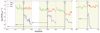 |
Fig. 4. Redshift evolution of the MBH accretion rates (Ṁ) for LDEs. We select four events for which the merger occurs at z ≳ 6 after taking into account the time delays due to DF. For each event, the red (blue) line refers to the primary (secondary) MBH, labelled BHp (BHs) in the figure, while the green line shows Ṁ of the new MBH resulting from the merger (BHnew). The black solid vertical lines show the times at which the merger occurs in the simulation, according to the instantaneous merging approximation. The vertical pink-dashed lines show the new redshifts at which the BHs merge after factoring in delays due to DF. The black arrows show the change in the merger redshifts upon considering time delays due to DF in post-processing. The yellow patches show the time span for which the selected BHs evolve without undergoing any other mergers between the two snapshots (the redshifts of the snapshots are depicted by vertical black-dotted lines). |
3.2. Observable properties of systems hosting merging MBHs
Starting from the intrinsic properties described above and following the formalism described in the Appendix B, we compute the following observable properties: the X-ray luminosity (LX), the total UV luminosity (LUV) and the corresponding UV magnitude (MAB) from stars and accreting BHs, the [CII] luminosity (LCII), and the far-infrared luminosity (LFIR). We report in Table B.2 the observable properties of the galaxies with which a merger is associated (in line with the events reported in Table B.1).
In Fig. 2, we show the PDFs of the aforementioned observational properties. The vertical lines represent the luminosity thresholds that we adopted to identify those sources that are more likely detectable with EM telescopes. In particular, for the UV, [CII], and FIR emissions, we consider the typical values found in the ALPINE survey (Le Fèvre et al. 2020) for z ∼ 5 − 6 galaxies (Béthermin et al. 2020; Faisst et al. 2020; Sommovigo et al. 2022). For the X-ray, we consider a threshold of LX ∼ 1042 erg s−1, which is close to the confusion limit of Athena (Aird et al. 2013) and is also expected to be reached by a Lynx-like9 instrument in ∼40 ks (see, e.g., Table 2 in Lops et al. 2023).
Hereafter, we denote EMDEs those events whose observable properties exceed at least one of the sensitivities of the EM telescopes considered. The red cyan-hatched region denotes those events that are both detectable with LISA and through EM telescopes, assuming instantaneous merger (Tot LDE ∧ EMDE). The red cross-hatched region indicates the EM and the LDEs at z ≳ 6 after accounting for DF effects. These are labelled as DF LDE ∧ EMDE in the figure.
Accounting for the DF effects, the fraction of LDE events that are EM detectable decreases from 31% to 21% in the X-ray, from 26% to 18% in the rest frame UV, from 32% to 21% in [CII], and from 45% to 32% in the FIR. In conclusion, only 20–30% of the total LDEs in the AGN_fid run is detectable with EM telescopes.10
3.3. Final selection of LDEs
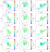 |
Fig. 5. 3D representation of the intrinsic properties of E31 at z = 6.8. Each box has a side of 20 pkpc and 1.2 pkpc along the z-, y-, and x-directions (in the left, middle, and right panel, respectively) for three different LOSs. First row: Gas density of the star-forming particles. The black circle identifies the region adopted to compute the intrinsic properties in Sect. 3.1, corresponding to 30% of the virial radius. The filled black circles represent the location of the MBHs in the simulation. In particular, the location of the merger event is denoted by a yellow-filled star. The location of the MBHs and of the merger event remain the same for all rows. To avoid clutter and to provide a better view of the host galaxy’s intrinsic properties, the black-filled circles and the yellow-filled star are presented only in the first row. Second row: Star formation rate of the SF particles. Third row: Gas metallicity of the SF particles. Fourth row: Gas velocity of the SF particles along the different LOS considered. |
The redshift distribution of the events as selected based on their observability with LISA and EM telescopes is shown in Fig. 3. In the left panel, all events (Tot) are shown in the blue-shaded region, the LDEs (Tot LDEs) in the cyan-shaded region, and the LDEs detectable with EM telescopes (Tot LDE ∧ EMDE) in the red cyan-hatched region. In the right panel, the PDFs of those MBHs whose merger occurs at z ≳ 6 after accounting for time delay effects (DF) are indicated by the dark-violet shaded region, the lilac shaded region shows the LDEs among the DF events (DF LDEs), while the red cross-hatched region (DF LDE ∧ EMDE) highlights the EMDEs among the DF LDEs.
We identify four events of particular interest due to their observational properties, each being the brightest in different EM bands: (LX, LUV, LCII, and LFIR) E19 at z = 6.5, E31 at z = 6.8, E36 at z = 7.0 and E52 at z = 8. In particular, E19 is the brightest in the LCII and LFIR bands, while E52 is the brightest in the LUV and LX band.
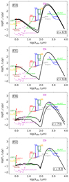 |
Fig. 6. Spectral energy distributions of the selected events: E19 at z = 6.5 (first row), E31 at z = 6.8 (second), E36 at z = 7.0 (third), and E52 (last) at z = 8.0, extracted from different LOSs shown as black solid lines in Fig. 5, from an aperture containing the SF region (rSF = 8.2, 7.4, 5.0, 4.8 kpc, respectively). The synthetic SEDs are compared with the sensitivities of various EM telescopes. The following are shown: LSST filters Z (dark green vertical line) and Y (red vertical line); Roman (brown horizontal line); JWST NIRCAM (orchid-coloured dots); JWST-MIRI (green curved line, for an exposure time of ∼3 h); Origins-like (grey horizontal lines, at 5σ in 1 hour), SPICA-like (red, blue, green boxes; yellow and magenta horizontal lines at 5σ in 1 h, represented by the top portions of the rectangles, and at 3σ by the lower sides of the rectangle; when the confusion limit is reached within an hour, sensitivities are indicated by the lines); ALMA (blue curved line, 10 h); and AtLAST (light green horizontal line). |
Figure 4 shows the accretion rate evolution of the MBHs involved in these events. We recall that these events are characterised by the following properties: (i) they are detectable with LISA with an S/N > 5; (ii) they are detectable with EM telescopes in at least one band (see Fig. 2); and (iii) the merging of the MBHs is expected to occur at z ≳ 6 after accounting for the time delay due to DF.
In Fig. 4, we show the accretion rate of the primary and secondary MBH before the merger, and the accretion rate of the MBH following the merger–namely, after the primary MBH swallows the secondary. As indicated, the resulting MBH inherits the location of the primary, and its total mass is defined by the sum of the mass of the primary and secondary MBH. We note that the post-merger accretion rate mostly aligns with that of the primary MBH before the merger; since it is more massive than the secondary MBH, the primary MBH dominates the accretion rate of the system.
3.4. 3D representation of intrinsic properties
We lastly showcase the spatial distribution of the intrinsic properties of the selected events at the snapshot closest to the numerical merger time11. Figure 5 shows the gas density (top panels), the SFR (second row), the gas metallicity (third row), and the gas velocity (bottom panels) of the star-forming particles relative to event 31 (E31) along three different lines of sight (LOS).
In Figs. A.1, A.2, and A.3, we report the same properties for the other three selected events. The black-filled circles represent the location of the BHs in the simulation. In particular, the location of the merger is denoted by a yellow-filled star. The solid circle indicates the region adopted to compute the intrinsic properties mentioned in Sect. 3.1 (i.e. 30% of the virial radius, hereafter denoted as the “SF region”: rSF = 8.2, 7.4, 5.0, 4.8 kpc, for E19, E31, E36, E52, respectively).
These figures clearly show that the star-forming particles are concentrated in regions of relatively high density (log ), which thus become the most metal-enriched (log
 ) reaching solar metallicity in the densest regions. In particular, for E31, the primary BH is located at a distance less than or close to the smoothing length (∼24 − 59 pc) from the densest (log
 ), more actively star-forming (log10 SFR = −1.5 M⊙ yr−1), and metal-enriched (log
![$ _{10} Z\,\rm[Z_{\odot}] = 0.58 $](/articles/aa/full_html/2025/06/aa52926-24/aa52926-24-eq11.gif) ) particle.
) particle.
From the bottom row, we observe the gas velocities of the star-forming particles along the z and y directions exhibit the dynamics of a rotating disc seen edge-on. The dynamics of the star-forming particles are further analysed in Sect. 5. Here, we likewise point to the presence of a disc-like velocity distribution in E52 along the x-direction, which aligns with recent ALMA results (Rowland et al. 2024).
4. EM signals from selected events
We performed the RT calculations following the set-up described in Sect. 2.3 and took into account the simulated volume centred on the galaxies hosting the events selected in Sect. 3.
4.1. Synthetic spectra
In Fig. 6, we show the SEDs resulting from our RT calculations for the selected events and compare them with the sensitivities of different EM telescopes. From this comparison, we find that E19 and E31 are detectable at short ( ) and long (
 ) wavelengths with any of the current or planned EM telescopes sensitive to these wavelengths (e.g. LSST, Euclid, Roman, JWST, and Origins for short wavelengths; ALMA and AtLAST for long wavelengths). In contrast, they are far below the detection limit of a SPICA-like telescope (see also PRIMA12). However, we note that our model does not include any dusty torus emissions. The detectability of LDEs at these wavelengths therefore depends on the possible presence and properties of a torus (i.e. dust mass and temperature; see e.g. Fig. 11 in Di Mascia et al. 2021). Similar considerations apply to E36 and E52; however these events are detectable only by JWST (and barely by Roman).
4.2. Synthetic maps of E31
Once we checked that the selected events were detectable in one or more EM bands, we investigated whether their emission properties differed from those of a typical AGN, powered by a single MBH. For this analysis, we focused on a specific event, E31. We predicted this event to occur at z = 6.8 (assuming instantaneous merger) or at z = 6.6 (when accounting for the time delay due to stellar DF), as shown in Fig. 4 (see the solid black vertical line associated with E31, and the dashed magenta vertical line indicated by the arrow).
In the panels of Fig. 7, the second and third rows show maps of the continuum emission predicted by our RT calculations for E31 in the wavelength ranges covered by LSST, JWST, and ALMA (left-most, middle, and right-most panels, respectively). In the same panels, coloured (black) circles represent the position of MBHs accreting at rates higher (lower) than Ṁ than 10−4 M⊙ yr−1. MBHs involved in the merger event are highlighted with white circles.
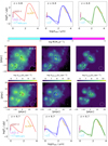 |
Fig. 7. Simulated maps (second and third row) in different observable bands and SEDs (first and bottom row) relative to event 31. From left to right we show the maps in the wavelength range of LSST (0.9–1.1 μm), NIRcam (3.8–5.1 μm), and ALMA (0.8–1.1 mm). Each map is convolved to match the angular resolution of the corresponding instruments considered: LSST (0.7″), NIRCAM (0.07″), and ALMA (0.5″). These values correspond to beam sizes of approximately 4 kpc, 0.4 kpc, and 3 kpc, respectively, at z ∼ 6.8, and are shown as white circles at the bottom of each panel in the second and third rows. The circles with white-coloured edges represent the coalescing MBHs, while the others represent the non-coalescing MBHs in the same halo. MBHs are coloured based on their mass accretion rates: MBHs with Ṁ < 10−4 M⊙ are represented in black, 10−4 M⊙ Ṁ < 10−3 M⊙ in cyan, and 10−3 M⊙ Ṁ < 10−2 M⊙ in blue. The MBHs with Ṁ > 10−1 M⊙ are represented in magenta. Small, medium, and large circles represent MBHs with masses MBH ≤ 105 M⊙, 105.5 M⊙ ≤ MBH ≤ 106 M⊙ and MBH > 106 M⊙, respectively. The top and bottom rows show the SEDs at z = 6.8 and z = 6.7, respectively. The left panel indicates the emission across the entire field of view. In the middle and right panels, square regions of 2 kpc and 800 pc, respectively, are selected around the merging BH (solid contour in the emission maps) to extract the SED (solid line in the SED plots). The same procedure is applied to other AGN in the field of view (dashed contour in the emission maps and dashed line in the SED plots). |
We also show, in the top and bottom panels, the SEDs at z = 6.8 and z = 6.7, corresponding to the redshifts before and after the merger. Specifically, we show the emission from the entire simulated field of view (left panel) as well as the emission associated with the merging BH and with other representative individual AGN–two at z = 6.8 and three at z = 6.7–in the field of view (middle and right panels). Comparing the SEDs of the post-merger BH against those of the isolated AGN, we find only marginal differences in the synthetic spectra, mostly in the mid-infrared band. However, in this region, the flux lies below the detection limit of the current or planned telescopes sensitive to this wavelength range.
We conclude that identifying an LDE from the continuum SEDs is not possible due to the absence of specific signatures from the merging MBHs.
5. Hα emission line from merging MBHs
High-z dual AGN, as recently suggested by JWST observations, have been discovered through double-peaked, broad emission Balmer lines (e.g. Maiolino 2024b; Übler et al. 2024). To investigate whether it would be possible to infer the presence of the accreting and merging MBHs in our selected events, we computed their Hα emission lines. The Hα line arises from recombinations occurring in the ISM of the host galaxy and in the broad line region (BLR) of the accreting BHs, producing a narrow component and two broad components, respectively.
The luminosity of the narrow component (in units of erg s−1) scales with the galaxy SFR (in units of M⊙ yr−1) according to the following equation from Kennicutt & Evans (2012):
Regarding its profile, the narrow component is shaped by the velocity distribution of the SF particles. To compute the profile of the line resulting from star formation, we first calculated the PDF of the velocities of the SF particles, weighted by their SFR. We then re-normalised the PDF so that its integrated flux matched LHα, as given by Eq. (8).
The luminosity of the broad components (LHαMBH) is instead proportional to the luminosity of the accreting BHs at 5100 Å (L5100), as given by the equation
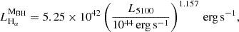
taken from Reines et al. (2013), where  , fbol = 0.1 (Lusso et al. 2012), and λEDD is the Eddington ratio, defined as the ratio between Ṁ and the Eddington accretion rate ṀEDD for each BH. The full width at half maximum of the broad components (FWHMBH) is lastly related to the above quantities through

taken from Reines et al. (2013). The line centroids associated with the BLR of the MBHs are offset from each other according to their relative velocity. Specifically, their relative position in the velocity space depends on the following relative velocities: vgal − vp as the relative velocity between the galaxy and the primary BH, and vp − vs as the relative velocity between the merging BHs.
To summarise, the profile of the Hα line was determined by the following quantities: SFR, velocity distribution of the SF particles, λEDD, p, Mp, λEDD, s, Ms, vgal − vp, and vp − vs. Predicted by our simulation13, these properties allowed us to properly compute the Hα emission line arising from our selected events.
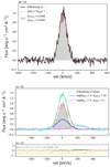 |
Fig. 8. Upper panel: Predicted Hα line profile from simulations for E36 along the x-direction. The grey-shaded region represents the result of our calculations. The solid black line denotes the total flux from the star-forming regions and the accreting primary and secondary MBHs. The red-dotted line shows the contribution only from the SF. To simulate noise, we add to our simulated spectra (in velocity bins of Δ v = 5 km s−1) a random number extracted by a Gaussian distribution with zero mean and a standard deviation of |

5.1. Synthetic Hα emission line from the selected events
Figure D.1 presents the Hα lines predicted by our simulations for the four selected events (from top to bottom: E19, E31, E36, and E52) along different LOSs: the z-, y-, and x-directions are displayed in the left, middle, and right panels, respectively. The top panel of Fig. 8 shows the specific case of E36 along the x-direction.
From a visual inspection of Fig. D.1 we find that the Hα emission line can exhibit very different profiles, depending on the event and the LOS considered: (i) a single-peaked shape (e.g. E36 along the three LOSs, E31 and E52 along the x and y directions, respectively); (ii) a double-peaked shape (e.g. E31 along the z and y directions, and E52 along the x-direction), consistent with the findings at the end of Sect. 3.4, where the gas velocity distribution along these directions resembles the dynamics of a rotating disc seen edge-on14; and (iii) a complex, multi-peaked structure (e.g. E19 along the three directions), similar to the “Disturbed Disk” stage analysed in Kohandel et al. (2020), where multiple star-forming clumps of gas perturbs the main galaxy disc (see Fig. A.1).
Regardless of the shape of the Hα line, the total flux (e.g. the black solid line in Fig. 8) always matches the flux arising from the star-forming regions (red dotted line) along all the LOSs and events considered. This means that the merging MBHs in our simulation are not accreting efficiently enough to leave any signature in the synthetic Hα line.
5.2. Boosting the accretion rates and masses of the MBHs
In the previous subsection, we concluded that the properties of our simulated systems were such that no signature of merging MBHs could be seen from the Hα profile. To generalise this result, we asked ourselves how efficiently two merging MBHs ought to accrete in order to be detectable.
To answer this question, we re-simulated the Hα line, keeping constant the contribution from the SFR and artificially boosting the accretion rates and masses of the merging MBHs (both in the primary and in the secondary). For simplicity’s sake, we restricted the analysis to a single event and to a single LOS. We chose E36 and the LOS along the x-direction since, in this case, the Hα line resembles neither the dynamics of a rotating disc in the edge-on view nor a “Disturbed Disk” stage.
The results of this experiment are shown in the bottom panel of Fig. 8 for E36 along the x-direction, considering equal-massed MBHs and boosted accretion rates. Figure D.2 presents results for different combinations of the MBH masses and accretion rates: in the left column, we keep the same MBH masses as in the E36 merger and vary their accretion rates from Eddington (λEDD, p = λEDD, s = 1) up to 10× Eddington; in the right column, we repeat the same exercise for the accretion rate but consider a primary MBH that is 10× more massive than the original one. From Fig. D.2, it is clear (and obvious) that the more the MBHs accrete and the more they are massive, the larger the deviation from the original Hα line. The issue here is whether or not we would be able to infer the presence of the two accreting MBHs even in these extreme cases.
To understand this issue, we adopted a procedure similar to the one described in Gallerani et al. (2018, see also Carniani et al. 2024), developed to infer the presence of outflowing gas from the shape of the [CII] (Hα) emission line. This method is based on analysing the residuals obtained by subtracting the best-fitting model from the emission line data. We thus fitted our simulated Hα lines both with a single Gaussian (SG) and a double Gaussian (DG) profile. The green and orange lines in the bottom panel of Fig. 8 and in Fig. D.2 report the best fitting results, assuming an SG and a DG profile, respectively. In the bottom inset of each panel, we further report the residual of the best-fitting procedure, along with the random noise added to the synthetic spectrum.
To measure the goodness of the fit, we applied the two-sample Kolmogorov-Smirnov (K-S) test (Kolmogorov 1933; Smirnov 1948) to our simulated data, and we computed the K-S probability (pKS). Specifically, we applied the two-sample KS test to compare the cumulative distribution function (CDF) of the SG residual with that of the noise, and similarly, the CDF of the DG residual with the CDF of the noise, in order to test whether the residuals come from the same random distribution used to simulate the noise. We note that, according to the K-S test, two samples are not drawn from the same underlying distribution if pKS < 0.05. We report the results of the K-S test in the bottom insets of each figure, along with the best-fit parameters, where the amplitudes of the Gaussians are in units of 10−19 erg s−1 cm−2 A−1. We find that, even in the case where λEDD, p = λEDD, s = 1 (top panels of Fig. D.2), the Hα line can be well fitted with an SG profile. In all other cases, including the one reported in the bottom panel of Fig. 8, the extreme accretion rates considered cause the profile to deviate in a statistically significant way from an SG profile (pKS, SG < 0.05). However, we also find that, in all cases, a DG profile is sufficient to provide a good fit to the synthetic spectra (pKS, DG > 0.05).
To summarise, the presence of two accreting MBHs would be difficult to infer even in very extreme (i.e. rare) circumstances (λEDD ∼ 5 − 10).
We thus conclude that the combined detection of GW and EM signals from z ≳ 6 MBHs is challenging (if not impossible) not only because of the poor sky-localization (∼10 deg2) provided by LISA but also because the loudest GW emitters (MBH ∼ 105−6 M⊙) are not massive enough to leave significant signatures (e.g. extended wings) in the emission lines arising from their BLRs.
6. Summary and discussion
In this work, we adopted a zoom-in cosmological hydrodynamical simulation of galaxy formation and BH co-evolution, based on the GADGET-3 code, zoomed-in on a Mh ∼ 1012 M⊙ DM halo at z = 6, which hosts a fast accreting (Ṁ ∼ 35 M⊙ yr−1) SMBH (MBH ∼ 109 M⊙) and a star-forming galaxy (SFR ∼ 100 M⊙ yr−1). Following the SMBH formation backwards in time, we identified the merger events that contributed to its formation and focused our analysis on those detectable with LISA which, after accounting for the delay due to the DF in the MBH coalescence, still occur at z ≳ 6. These events arise from the coalescence of MBHs with masses MBH ∼ 105−6 M⊙.
We then investigated the intrinsic properties of the host galaxies of these LDEs, finding the following typical properties: BHAR Ṁ ∼ 0.01 M⊙ yr−1, SFR ∼ 10−40 M⊙ yr−1, metallicity Z ∼ 0.4 − 0.6 Z⊙, dust mass Mdust ∼ 105 − 106 M⊙, stellar mass Mstellar ∼ 109−1010 M⊙, and gas mass Mgas ∼ 109−1010 M⊙. Among these LDEs, we selected those which, based on their intrinsic properties, were expected to be bright in one or more EM bands (e.g. rest-frame X-ray, UV, and FIR). We find that ∼20–30% of the LDEs are also detectable with EM telescopes.
We post-processed these events with dust radiative transfer calculations to make accurate predictions about their SEDs and continuum maps in the JWST to ALMA wavelength range. By comparing the spectra arising from the galaxies hosting the merging MBHs with those arising from the AGN powered by single accreting BHs, we find it impossible to identify an LDE from the continuum SEDs because of the absence of specific imprints from the merging MBHs.
Lastly, we computed the profile of the Hα line arising from LDEs, accounting for the contribution from both their star-forming regions and the accreting MBHs. We find that even in the extreme case where both MBHs accrete at super-Eddington rates, the shape of the Hα line does not deviate significantly from that produced from star formation only.
We conclude that the combined detection of GW and EM signals from z ≳ 6 MBHs is challenging, if not impossible, not only due to the poor sky-localization (∼10 deg2) provided by LISA, but also because the loudest GW emitters (MBH ∼ 105−6 M⊙) are not massive enough to leave significant signatures (e.g. extended wings) in the emission lines arising from the BLR.
MUSIC-Multiscale Initial Conditions for Cosmological Simulations: https://bitbucket.org/ohahn/music
A Λ cold dark matter (ΛCDM) cosmology was assumed with the following parameters (Planck Collaboration XIII 2016): ΩM, 0 = 0.3089, ΩΛ, 0 = 0.6911, ΩB, 0 = 0.0486, H0 = 67.74 km s−1 Mpc−1.
The chosen value of the radiative efficiency corresponds to the minimum accretion efficiency of a non-spinning BH surrounded by an accretion disc (Shakura & Sunyaev 1973) and is also compatible with the results of Sądowski & Gaspari (2017) and Trakhtenbrot et al. (2017).
Version 8, http://www.skirt.ugent.be
Throughout this paper, gas metallicity is expressed in solar units using Z⊙ = 0.013 as a reference value (Asplund et al. 2009).
In Appendix C, we compare the observable properties of host galaxies of LDEs with those of hosts of non-merging MBHs.
Ideally, to describe the properties of the host galaxy and MBH during a merger event, we should account for the merger time after including DF effects. However, under the assumption of instantaneous merger, the last point at which the galaxy and the MBH properties are self-consistently computed is at the numerical merger time. Thus, from a physical standpoint, it is appropriate to consider the snapshot closest to the numerical merger time.
The relative velocities between the primary and secondary MBHs were computed at those timesteps when the first–but not the second–merger condition was met. See condition (i) and (ii) in Sect. 2.1.2, respectively.
The spectral profile of a disc seen edge-on (face-on) is characterised by a double- (single-) peaked shape (e.g. Elitzur et al. 2012).
Acknowledgments
SG acknowledges support from the ASI-INAF n. 2018-31-HH.0 grant and PRIN-MIUR 2017. MV is supported by the Italian Research Center on High Performance Computing, Big Data and Quantum Computing (ICSC), project funded by European Union – NextGenerationEU – and National Recovery and Resilience Plan (NRRP) – Mission 4 Component 2, within the activities of Spoke 3, Astrophysics and Cosmos Observations, and by the INFN Indark Grant.
References
- Abbott, B. P., Abbott, R., Abbott, T. D., et al. 2018, Living Rev. Relativ., 21, 3 [Google Scholar]
- Agazie, G., Anumarlapudi, A., Archibald, A. M., et al. 2023, ApJ, 952, L37 [NASA ADS] [CrossRef] [Google Scholar]
- Aird, J., Comastri, A., Brusa, M., et al. 2013, arXiv e-prints [arXiv:1306.2325] [Google Scholar]
- Amaro-Seoane, P., Andrews, J., Arca Sedda, M., et al. 2023, Living Rev. Relativ., 26, 2 [NASA ADS] [CrossRef] [Google Scholar]
- Antoniadis, J., Arzoumanian, Z., Babak, S., et al. 2022, MNRAS, 510, 4873 [NASA ADS] [CrossRef] [Google Scholar]
- Armitage, P. J., & Natarajan, P. 2002, ApJ, 567, L9 [NASA ADS] [CrossRef] [Google Scholar]
- Asplund, M., Grevesse, N., Sauval, A. J., & Scott, P. 2009, ARA&A, 47, 481 [NASA ADS] [CrossRef] [Google Scholar]
- Baes, M., Davies, J. I., Dejonghe, H., et al. 2003, MNRAS, 343, 1081 [NASA ADS] [CrossRef] [Google Scholar]
- Bardati, J., Ruan, J. J., Haggard, D., & Tremmel, M. 2024, ApJ, 961, 34 [Google Scholar]
- Begelman, M. C., Blandford, R. D., & Rees, M. J. 1980, Nature, 287, 307 [Google Scholar]
- Behrens, C., Pallottini, A., Ferrara, A., Gallerani, S., & Vallini, L. 2018, MNRAS, 477, 552 [NASA ADS] [CrossRef] [Google Scholar]
- Béthermin, M., Fudamoto, Y., Ginolfi, M., et al. 2020, A&A, 643, A2 [Google Scholar]
- Bhatt, M., Gallerani, S., Ferrara, A., et al. 2024, A&A, 686, A141 [NASA ADS] [CrossRef] [EDP Sciences] [Google Scholar]
- Bogdanović, T., Miller, M. C., & Blecha, L. 2022, Living Rev. Relativ., 25, 3 [Google Scholar]
- Bondi, H. 1952, MNRAS, 112, 195 [Google Scholar]
- Bondi, H., & Hoyle, F. 1944, MNRAS, 104, 273 [Google Scholar]
- Booth, C. M., & Schaye, J. 2009, MNRAS, 398, 53 [Google Scholar]
- Bosman, S. E. I., Álvarez Márquez, J., Colina, L., et al. 2023, arXiv e-prints [arXiv:2307.14414] [Google Scholar]
- Bruzual, G., & Charlot, S. 2003, MNRAS, 344, 1000 [NASA ADS] [CrossRef] [Google Scholar]
- Camps, P., & Baes, M. 2015, Astron. Comput., 9, 20 [Google Scholar]
- Carniani, S., Gallerani, S., Vallini, L., et al. 2019, MNRAS, 489, 3939 [NASA ADS] [Google Scholar]
- Carniani, S., Venturi, G., Parlanti, E., et al. 2024, A&A, 685, A99 [NASA ADS] [CrossRef] [EDP Sciences] [Google Scholar]
- Carr, B. J., & Green, A. M. 2025, The History of Primordial Black Holes (Singapore: Springer Nature), 3 [CrossRef] [Google Scholar]
- Chakraborty, S., Gallerani, S., Zana, T., et al. 2023, MNRAS, 523, 758 [NASA ADS] [CrossRef] [Google Scholar]
- Chandrasekhar, S. 1943, ApJ, 97, 255 [Google Scholar]
- Damiano, A., Valentini, M., Borgani, S., et al. 2024, A&A, 692, A81 [NASA ADS] [CrossRef] [EDP Sciences] [Google Scholar]
- DeGraf, C., Sijacki, D., Di Matteo, T., et al. 2021, MNRAS, 503, 3629 [NASA ADS] [CrossRef] [Google Scholar]
- Di Mascia, F., Gallerani, S., Behrens, C., et al. 2021, MNRAS, 503, 2349 [NASA ADS] [CrossRef] [Google Scholar]
- Dong-Páez, C. A., Volonteri, M., Beckmann, R. S., et al. 2023, A&A, 676, A2 [NASA ADS] [CrossRef] [EDP Sciences] [Google Scholar]
- Draine, B. 2003, ARA&A, 41, 241 [NASA ADS] [CrossRef] [Google Scholar]
- Draine, B. T. 2004, Astrophysics of Dust in Cold Clouds (Berlin, Heidelberg: Springer), 213 [Google Scholar]
- Draine, B. T., & Salpeter, E. E. 1979, ApJ, 231, 77 [NASA ADS] [CrossRef] [Google Scholar]
- Draine, B. T., Dale, D. A., Bendo, G., et al. 2007, ApJ, 663, 866 [NASA ADS] [CrossRef] [Google Scholar]
- Edgar, R. 2004, New Astron. Rev., 48, 843 [CrossRef] [Google Scholar]
- Elitzur, M., Asensio Ramos, A., & Ceccarelli, C. 2012, MNRAS, 422, 1394 [NASA ADS] [CrossRef] [Google Scholar]
- EPTA Collaboration, InPTA Collaboration (Antoniadis, J., et al.) 2023, A&A, 678, A50 [CrossRef] [EDP Sciences] [Google Scholar]
- Faisst, A. L., Schaerer, D., Lemaux, B. C., et al. 2020, ApJS, 247, 61 [NASA ADS] [CrossRef] [Google Scholar]
- Fan, X., Bañados, E., & Simcoe, R. A. 2023, ARA&A, 61, 373 [NASA ADS] [CrossRef] [Google Scholar]
- Ferrara, A., Salvadori, S., Yue, B., & Schleicher, D. 2014, MNRAS, 443, 2410 [NASA ADS] [CrossRef] [Google Scholar]
- Flanagan, É. É., & Hughes, S. A. 1998, Phys. Rev. D, 57, 4535 [Google Scholar]
- Furtak, L. J., Labbé, I., Zitrin, A., et al. 2024, Nature, 628, 57 [NASA ADS] [CrossRef] [Google Scholar]
- Gallerani, S., Pallottini, A., Feruglio, C., et al. 2018, MNRAS, 473, 1909 [Google Scholar]
- Goulding, A. D., Greene, J. E., Setton, D. J., et al. 2023, ApJ, 955, L24 [NASA ADS] [CrossRef] [Google Scholar]
- Greene, J. E., Labbe, I., Goulding, A. D., et al. 2024, ApJ, 964, 39 [CrossRef] [Google Scholar]
- Haehnelt, M. G., & Rees, M. J. 1993, MNRAS, 263, 168 [Google Scholar]
- Hahn, O., & Abel, T. 2011, MNRAS, 415, 2101 [Google Scholar]
- Hopkins, P. F., Richards, G. T., & Hernquist, L. 2007, ApJ, 654, 731 [Google Scholar]
- Hoyle, F., & Lyttleton, R. A. 1939, Proc. Cambridge Philos. Soc., 35, 405 [Google Scholar]
- Izquierdo-Villalba, D., Colpi, M., Volonteri, M., et al. 2023, A&A, 677, A123 [NASA ADS] [CrossRef] [EDP Sciences] [Google Scholar]
- Jeon, J., Bromm, V., Liu, B., & Finkelstein, S. L. 2025, ApJ, 979, 127 [Google Scholar]
- Kennicutt, R. C., & Evans, N. J. 2012, ARA&A, 50, 531 [NASA ADS] [CrossRef] [Google Scholar]
- Kohandel, M., Pallottini, A., Ferrara, A., et al. 2020, MNRAS, 499, 1250 [Google Scholar]
- Kokorev, V., Fujimoto, S., Labbe, I., et al. 2023, ApJ, 957, L7 [NASA ADS] [CrossRef] [Google Scholar]
- Kolmogorov, A. 1933, Inst. Ital. Attuari Giorn, 4, 83 [Google Scholar]
- Kovács, O. E., Bogdán, Á., Natarajan, P., et al. 2024, ApJ, 965, L21 [CrossRef] [Google Scholar]
- Krolik, J. H., Volonteri, M., Dubois, Y., & Devriendt, J. 2019, ApJ, 879, 110 [NASA ADS] [CrossRef] [Google Scholar]
- Larson, R. L., Finkelstein, S. L., Kocevski, D. D., et al. 2023, ApJ, 953, L29 [NASA ADS] [CrossRef] [Google Scholar]
- Latif, M. A., & Ferrara, A. 2016, PASA, 33, e051 [NASA ADS] [CrossRef] [Google Scholar]
- Le Fèvre, O., Béthermin, M., Faisst, A., et al. 2020, A&A, 643, A1 [Google Scholar]
- Lops, G., Izquierdo-Villalba, D., Colpi, M., et al. 2023, MNRAS, 519, 5962 [NASA ADS] [CrossRef] [Google Scholar]
- Luo, J., Chen, L.-S., Duan, H.-Z., et al. 2016, Classical Quantum Gravity, 33, 035010 [NASA ADS] [CrossRef] [Google Scholar]
- Lusso, E., Comastri, A., Simmons, B. D., et al. 2012, MNRAS, 425, 623 [Google Scholar]
- Lynden-Bell, D. 1969, Nature, 223, 690 [NASA ADS] [CrossRef] [Google Scholar]
- Maiolino, R., et al. 2024a, Nature, 627, 59 [Erratum: Nature 630, E2 (2024)] [NASA ADS] [CrossRef] [Google Scholar]
- Maiolino, R., et al. 2024b, A&A, 691, A145 [NASA ADS] [CrossRef] [EDP Sciences] [Google Scholar]
- Manchester, R. N., Hobbs, G., Bailes, M., et al. 2013, Publ. Astron. Soc. Aust., 30, e017 [Google Scholar]
- Mangiagli, A., Klein, A., Bonetti, M., et al. 2020, Phys. Rev. D, 102, 084056 [NASA ADS] [CrossRef] [Google Scholar]
- Mangiagli, A., Caprini, C., Volonteri, M., et al. 2022, Phys. Rev. D, 106, 103017 [NASA ADS] [CrossRef] [Google Scholar]
- Matsuoka, Y., Izumi, T., Onoue, M., et al. 2024, ApJ, 965, L4 [Google Scholar]
- Mayer, L., & Bonoli, S. 2019, Rep. Prog. Phys., 82, 016901 [Google Scholar]
- Murante, G., Monaco, P., Giovalli, M., Borgani, S., & Diaferio, A. 2010, MNRAS, 405, 1491 [NASA ADS] [Google Scholar]
- Murante, G., Monaco, P., Borgani, S., et al. 2015, MNRAS, 447, 178 [NASA ADS] [CrossRef] [Google Scholar]
- Murphy, E. J., Condon, J. J., Schinnerer, E., et al. 2011, ApJ, 737, 67 [Google Scholar]
- Oke, J. B., & Gunn, J. E. 1983, ApJ, 266, 713 [NASA ADS] [CrossRef] [Google Scholar]
- Ostriker, E. C. 1999, ApJ, 513, 252 [Google Scholar]
- Pacucci, F., Nguyen, B., Carniani, S., Maiolino, R., & Fan, X. 2023, ApJ, 957, L3 [CrossRef] [Google Scholar]
- Pillepich, A., Springel, V., Nelson, D., et al. 2018, MNRAS, 473, 4077 [Google Scholar]
- Planck Collaboration XIII. 2016, A&A, 594, A13 [NASA ADS] [CrossRef] [EDP Sciences] [Google Scholar]
- Press, W. H., & Schechter, P. 1974, ApJ, 187, 425 [Google Scholar]
- Reines, A. E., Greene, J. E., & Geha, M. 2013, ApJ, 775, 116 [Google Scholar]
- Rowland, L. E., Hodge, J., Bouwens, R., et al. 2024, MNRAS, 535, 2068 [Google Scholar]
- Ruan, W.-H., Guo, Z.-K., Cai, R.-G., & Zhang, Y.-Z. 2020, Int. J. Mod. Phys. A, 35, 2050075 [NASA ADS] [CrossRef] [Google Scholar]
- Sądowski, A., & Gaspari, M. 2017, MNRAS, 468, 1398 [CrossRef] [Google Scholar]
- Saeedzadeh, V., Babul, A., Mukherjee, S., et al. 2024, ArXiv e-prints [arXiv:2403.17076] [Google Scholar]
- Schaye, J., Crain, R. A., Bower, R. G., et al. 2015, MNRAS, 446, 521 [Google Scholar]
- Schneider, R., Valiante, R., Trinca, A., et al. 2023, MNRAS, 526, 3250 [NASA ADS] [CrossRef] [Google Scholar]
- Schutz, B. F. 1986, Nature, 323, 310 [Google Scholar]
- Sesana, A., & Khan, F. M. 2015, MNRAS, 454, L66 [Google Scholar]
- Sesana, A., Haardt, F., Madau, P., & Volonteri, M. 2004, ApJ, 611, 623 [NASA ADS] [CrossRef] [Google Scholar]
- Shakura, N. I., & Sunyaev, R. A. 1973, A&A, 500, 33 [NASA ADS] [Google Scholar]
- Shen, X., Hopkins, P. F., Faucher-Giguère, C.-A., et al. 2020, MNRAS, 495, 3252 [Google Scholar]
- Smirnov, N. 1948, Ann. Math. Stat., 19, 279 [CrossRef] [Google Scholar]
- Sommovigo, L., Ferrara, A., Carniani, S., et al. 2022, MNRAS, 517, 5930 [NASA ADS] [CrossRef] [Google Scholar]
- Springel, V. 2005, MNRAS, 364, 1105 [Google Scholar]
- Steinborn, L. K., Dolag, K., Hirschmann, M., Prieto, M. A., & Remus, R.-S. 2015, MNRAS, 448, 1504 [Google Scholar]
- Tarafdar, P., Nobleson, K., Rana, P., et al. 2022, Publ. Astron. Soc. Aust., 39, e053 [Google Scholar]
- Tornatore, L., Borgani, S., Dolag, K., & Matteucci, F. 2007, MNRAS, 382, 1050 [Google Scholar]
- Trakhtenbrot, B., Lira, P., Netzer, H., et al. 2017, ApJ, 836, 8 [NASA ADS] [CrossRef] [Google Scholar]
- Trinca, A., Schneider, R., Maiolino, R., et al. 2023, MNRAS, 519, 4753 [NASA ADS] [CrossRef] [Google Scholar]
- Übler, H., Maiolino, R., Pérez-González, P. G., et al. 2024, MNRAS, 531, 355 [CrossRef] [Google Scholar]
- Valentini, M., Murante, G., Borgani, S., et al. 2017, MNRAS, 470, 3167 [CrossRef] [Google Scholar]
- Valentini, M., Bressan, A., Borgani, S., et al. 2018, MNRAS, 480, 722 [Google Scholar]
- Valentini, M., Borgani, S., Bressan, A., et al. 2019, MNRAS, 485, 1384 [NASA ADS] [CrossRef] [Google Scholar]
- Valentini, M., Murante, G., Borgani, S., et al. 2020, MNRAS, 491, 2779 [Google Scholar]
- Valentini, M., Gallerani, S., & Ferrara, A. 2021, MNRAS, 507, 1 [NASA ADS] [CrossRef] [Google Scholar]
- Valiante, R., Agarwal, B., Habouzit, M., & Pezzulli, E. 2017, PASA, 34, e031 [Google Scholar]
- Valiante, R., Colpi, M., Schneider, R., et al. 2021, MNRAS, 500, 4095 [Google Scholar]
- Vallini, L., Gallerani, S., Ferrara, A., & Baek, S. 2013, MNRAS, 433, 1567 [NASA ADS] [CrossRef] [Google Scholar]
- Vallini, L., Gallerani, S., Ferrara, A., Pallottini, A., & Yue, B. 2015, ApJ, 813, 36 [NASA ADS] [CrossRef] [Google Scholar]
- Verbiest, J. P. W., Lentati, L., Hobbs, G., et al. 2016, MNRAS, 458, 1267 [Google Scholar]
- Volonteri, M., Haardt, F., & Madau, P. 2003, ApJ, 582, 559 [Google Scholar]
- Volonteri, M., Pfister, H., Beckmann, R. S., et al. 2020, MNRAS, 498, 2219 [Google Scholar]
- Volonteri, M., Habouzit, M., & Colpi, M. 2021, Nat. Rev. Phys., 3, 732 [NASA ADS] [CrossRef] [Google Scholar]
- Weinberger, R., Springel, V., Hernquist, L., et al. 2017, MNRAS, 465, 3291 [Google Scholar]
- Weingartner, J. C., & Draine, B. T. 2001, ApJ, 548, 296 [Google Scholar]
- Wise, J. H., Regan, J. A., O’Shea, B. W., et al. 2019, Nature, 566, 85 [NASA ADS] [CrossRef] [Google Scholar]
- Xu, H., Chen, S., Guo, Y., et al. 2023, Res. Astron. Astrophys., 23, 075024 [CrossRef] [Google Scholar]
- Yu, Q., & Tremaine, S. 2002, MNRAS, 335, 965 [NASA ADS] [CrossRef] [Google Scholar]
- Yue, B., Ferrara, A., Salvaterra, R., Xu, Y., & Chen, X. 2013, MNRAS, 433, 1556 [Google Scholar]
- Zana, T., Gallerani, S., Carniani, S., et al. 2022, MNRAS, 513, 2118 [NASA ADS] [CrossRef] [Google Scholar]
- Ziparo, F., Gallerani, S., & Ferrara, A. 2025, JCAP, 04, 040 [Google Scholar]
Appendix A: 3D representation of intrinsic properties for the other events
In Fig. 5 we showed the intrinsic properties (gas density, SFR, gas metallicity and gas velocity) relative to E31. In this section we show the same properties for events E19, E36, E52.
Intrinsic properties of GW host galaxies.
Appendix B: Observable properties
B.1. UV and X-ray Luminosity
We compute the UV luminosity considering the contributions from both stars and accreting MBHs:

For what concerns stars, we adopt the SFR-LUV, * relation derived by Murphy et al. (2011):
The AGN UV luminosity is instead computed as follows:
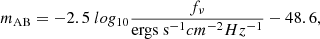
where the bolometric luminosity Lbol is related to the accretion rate of the MBH,  , ϵr is the radiative efficiency, and fUV represents the UV bolometric correction parametrized as in Hopkins et al. (2007):
where, c1 = 1.862, k1 = −0.361, c2 = 4.870, k2 = −0.0063 (Shen et al. 2020).
At λ = 1450 Å, we can relate the AGN UV luminosity to the emitted UV luminosity density as:
The observed UV flux density can be then expressed as:

where dL is the luminosity distance of the source. The observed (apparent) UV magnitude can be derived from the flux density (Oke & Gunn 1983):
and the apparent (mAB) and absolute magnitude (MAB) are related as:
where μ is the distance modulus.
Similarly, we compute the X-ray luminosity
as LX = fXLbol, with the following parameters for the bolometric correction: c1 = 4.073, k1 = −0.026, c2 = 12.6, k2 = 0.278 (Hopkins et al. 2007). These bolometric corrections well reproduce the X-ray SED template proposed by Shen et al. (2020).
B.2. Far-infrared luminosity
The FIR luminosity associated with dust emission in the optically thin regime can be computed as follows (Carniani et al. 2019):
where Bν(Tdust) is the Planck function associated to the dust component at temperature Tdust:
and
where we assume the dust emissivity index β = 2.2, and the mass absorption coefficient k0 = 34.7 at a frequency ν0 that corresponds to λ = 100 μm (Draine 2003, 2004). These parameters fit the dust emissivity in the FIR band kν of the Small Magenallic Cloud. The dust mass is given by Mdust = fd × Mmetals, with fd = 0.1 and Mmetals = Z × Mgas, as described in Sect. 2.3.1.
B.3. [CII] Luminosity
To compute the [CII] luminosity LCII we adopt the following fitting formula proposed by Yue et al. (2013) and based on the ISM sub-grid models by Vallini et al. (2013, 2015):
where LCII, SFR, and Z are given in units of L⊙, M⊙yr−1 and Z⊙, respectively.
Observable properties of GW host galaxies.
Appendix C: Comparison with non-merging MBH
In this section we compare the observable properties of LDEs with MBHs in the same mass range, seeded in a host galaxy, which are not associated with any mergers (non-merging MBHs, NMBHs). In Fig. C.1, we show in the left column, the observable properties of all MBHs associated with a host galaxy which are not involved in any coalescence. Whereas, in the right column we show the observable properties of host galaxies of LDEs. We also show the EM bright events in both cases as described in Sect. 3.2. We note that in our simulations, only ∼0.3% of all MBHs eventually result in mergers. From fig. C.1, we can see there is no significant difference in the distribution of observable properties of merging MBHs detectable by LISA and non-merging MBHs. Hence, within our simulation limits, we cannot distinguish LDE population from NMBH population based on their observable EM properties.
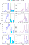 |
Fig. C.1. PDFs of different observable properties of MBHs associated with a host galaxy which eventually merge within the LISA band (purple dashed) and do not merge referred to as NMBH, (blue solid) at z > 6. In the left column, the cyan bars represent the non-merging MBHs which are detectable by EM telescopes and in the right column, the lavender bars represent the LDEs which are also EMDEs (see also Fig. 2). We report results for different wavelength bands: X-ray (first row), UV (second row), [CII] (third row), FIR (bottom row). In each panel, we also report the average and 1σ values of EM bright events. |
Appendix D: Hα emission line from merging MBHs of selected events
In this section we first report the predicted Hα profiles for all four selected events (E19, E31, E36 and E52) along LOS in the x, y and z direction in Fig. D.1. Furthermore, we show the resimulated Hα line profiles for E36 in x-direction in Fig. D.2, when we consider various MBH mass and accretion rates. We have provided a detailed analysis of this in Sects. 5.1 and 5.2.
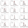 |
Fig. D.1. Predicted Hα line profiles from simulations for E19, E31, E36 and E52 (first, second, third, and last rows, respectively) shown along LOS in the z, y, and x (first, second and last columns, respectively) directions. The grey-shaded regions represent the calculated results. The solid black lines indicate the total flux (from SF, the accreting primary and secondary MBHs) along with the noise component and the red-dotted lines show the contribution only from SF. |
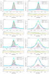 |
Fig. D.2. Re-simulated Hα profile for E36 in the LOS along the x-direction. The left column shows results for constant masses of MBHs but varying accretion rates. For the same values of the accretion rates as shown in the left column, we show the results when the primary MBH is ten times more massive than the secondary MBH. The blue (pink) dashed line represents the contribution from primary (secondary) MBH. The bottom inset in each panel refers to the added random noise in the synthetic spectrum along with the residual of the best-fitting model as explained in Sect. 5.2. |
All Tables
All Figures
|
Fig. 1. The PDFs of different intrinsic properties of LDEs associated with a host galaxy before (purple dashed line) and after (black solid line) adding time delay due to DF at z > 6. In each panel, the lavender bars represent the LDEs, which are also EMDEs for all events (see Sect. 3.2), while the red region represents the same for the events that occur after accounting for time delays due to DF. In the top panel from left to right, respectively: Chirp mass of LISA events, stellar mass, SFRs, and sSFRs of the host galaxies. In the bottom panel from left to right, respectively: total accretion rates of LISA events, gas mass, metallicity, and dust mass of the host galaxies. Mass and metallicities are represented in solar units. |
| In the text | |
|
Fig. 3. Probability distribution functions of all merger events and all LDEs (left panel), and DF events and DF LDEs (right panel). In the left panel, the blue solid line represents the total number of merger events in our AGN_fid run. The purple dashed line represents the LDEs in the AGN_fid, while the lavender area further denotes the LDEs which are also detectable in the UV, X-ray, CII, and/or FIR bands by JWST, LynX, and ALMA. In the right panel, the grey area represents the mergers that take place at z > 6 after taking into account the time delay due to DF. The black solid line shows the LDEs of these aforementioned mergers, while the red area represents the LDEs and EMDEs from these mergers. |
| In the text | |
|
Fig. 2. PDF comparison of different observable properties of LDEs (dashed purple line), after adding the time delay due to DF at z > 6 (black solid line) for follow-up observations in different wavelength bands: X-ray (left most), UV (second), [CII] (third), and FIR (right most panel). The colours correspond to those in Fig. 1. |
| In the text | |
|
Fig. 4. Redshift evolution of the MBH accretion rates (Ṁ) for LDEs. We select four events for which the merger occurs at z ≳ 6 after taking into account the time delays due to DF. For each event, the red (blue) line refers to the primary (secondary) MBH, labelled BHp (BHs) in the figure, while the green line shows Ṁ of the new MBH resulting from the merger (BHnew). The black solid vertical lines show the times at which the merger occurs in the simulation, according to the instantaneous merging approximation. The vertical pink-dashed lines show the new redshifts at which the BHs merge after factoring in delays due to DF. The black arrows show the change in the merger redshifts upon considering time delays due to DF in post-processing. The yellow patches show the time span for which the selected BHs evolve without undergoing any other mergers between the two snapshots (the redshifts of the snapshots are depicted by vertical black-dotted lines). |
| In the text | |
|
Fig. 5. 3D representation of the intrinsic properties of E31 at z = 6.8. Each box has a side of 20 pkpc and 1.2 pkpc along the z-, y-, and x-directions (in the left, middle, and right panel, respectively) for three different LOSs. First row: Gas density of the star-forming particles. The black circle identifies the region adopted to compute the intrinsic properties in Sect. 3.1, corresponding to 30% of the virial radius. The filled black circles represent the location of the MBHs in the simulation. In particular, the location of the merger event is denoted by a yellow-filled star. The location of the MBHs and of the merger event remain the same for all rows. To avoid clutter and to provide a better view of the host galaxy’s intrinsic properties, the black-filled circles and the yellow-filled star are presented only in the first row. Second row: Star formation rate of the SF particles. Third row: Gas metallicity of the SF particles. Fourth row: Gas velocity of the SF particles along the different LOS considered. |
| In the text | |
|
Fig. 6. Spectral energy distributions of the selected events: E19 at z = 6.5 (first row), E31 at z = 6.8 (second), E36 at z = 7.0 (third), and E52 (last) at z = 8.0, extracted from different LOSs shown as black solid lines in Fig. 5, from an aperture containing the SF region (rSF = 8.2, 7.4, 5.0, 4.8 kpc, respectively). The synthetic SEDs are compared with the sensitivities of various EM telescopes. The following are shown: LSST filters Z (dark green vertical line) and Y (red vertical line); Roman (brown horizontal line); JWST NIRCAM (orchid-coloured dots); JWST-MIRI (green curved line, for an exposure time of ∼3 h); Origins-like (grey horizontal lines, at 5σ in 1 hour), SPICA-like (red, blue, green boxes; yellow and magenta horizontal lines at 5σ in 1 h, represented by the top portions of the rectangles, and at 3σ by the lower sides of the rectangle; when the confusion limit is reached within an hour, sensitivities are indicated by the lines); ALMA (blue curved line, 10 h); and AtLAST (light green horizontal line). |
| In the text | |
|
Fig. 7. Simulated maps (second and third row) in different observable bands and SEDs (first and bottom row) relative to event 31. From left to right we show the maps in the wavelength range of LSST (0.9–1.1 μm), NIRcam (3.8–5.1 μm), and ALMA (0.8–1.1 mm). Each map is convolved to match the angular resolution of the corresponding instruments considered: LSST (0.7″), NIRCAM (0.07″), and ALMA (0.5″). These values correspond to beam sizes of approximately 4 kpc, 0.4 kpc, and 3 kpc, respectively, at z ∼ 6.8, and are shown as white circles at the bottom of each panel in the second and third rows. The circles with white-coloured edges represent the coalescing MBHs, while the others represent the non-coalescing MBHs in the same halo. MBHs are coloured based on their mass accretion rates: MBHs with Ṁ < 10−4 M⊙ are represented in black, 10−4 M⊙ Ṁ < 10−3 M⊙ in cyan, and 10−3 M⊙ Ṁ < 10−2 M⊙ in blue. The MBHs with Ṁ > 10−1 M⊙ are represented in magenta. Small, medium, and large circles represent MBHs with masses MBH ≤ 105 M⊙, 105.5 M⊙ ≤ MBH ≤ 106 M⊙ and MBH > 106 M⊙, respectively. The top and bottom rows show the SEDs at z = 6.8 and z = 6.7, respectively. The left panel indicates the emission across the entire field of view. In the middle and right panels, square regions of 2 kpc and 800 pc, respectively, are selected around the merging BH (solid contour in the emission maps) to extract the SED (solid line in the SED plots). The same procedure is applied to other AGN in the field of view (dashed contour in the emission maps and dashed line in the SED plots). |
| In the text | |
|
Fig. 8. Upper panel: Predicted Hα line profile from simulations for E36 along the x-direction. The grey-shaded region represents the result of our calculations. The solid black line denotes the total flux from the star-forming regions and the accreting primary and secondary MBHs. The red-dotted line shows the contribution only from the SF. To simulate noise, we add to our simulated spectra (in velocity bins of Δ v = 5 km s−1) a random number extracted by a Gaussian distribution with zero mean and a standard deviation of |
| In the text | |
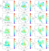 |
Fig. A.1. Same as Fig. 5 but for E19. |
| In the text | |
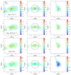 |
Fig. A.2. Same as Fig. 5 but for E36. |
| In the text | |
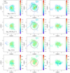 |
Fig. A.3. Same as Fig. 5 but for E52. |
| In the text | |
|
Fig. C.1. PDFs of different observable properties of MBHs associated with a host galaxy which eventually merge within the LISA band (purple dashed) and do not merge referred to as NMBH, (blue solid) at z > 6. In the left column, the cyan bars represent the non-merging MBHs which are detectable by EM telescopes and in the right column, the lavender bars represent the LDEs which are also EMDEs (see also Fig. 2). We report results for different wavelength bands: X-ray (first row), UV (second row), [CII] (third row), FIR (bottom row). In each panel, we also report the average and 1σ values of EM bright events. |
| In the text | |
|
Fig. D.1. Predicted Hα line profiles from simulations for E19, E31, E36 and E52 (first, second, third, and last rows, respectively) shown along LOS in the z, y, and x (first, second and last columns, respectively) directions. The grey-shaded regions represent the calculated results. The solid black lines indicate the total flux (from SF, the accreting primary and secondary MBHs) along with the noise component and the red-dotted lines show the contribution only from SF. |
| In the text | |
|
Fig. D.2. Re-simulated Hα profile for E36 in the LOS along the x-direction. The left column shows results for constant masses of MBHs but varying accretion rates. For the same values of the accretion rates as shown in the left column, we show the results when the primary MBH is ten times more massive than the secondary MBH. The blue (pink) dashed line represents the contribution from primary (secondary) MBH. The bottom inset in each panel refers to the added random noise in the synthetic spectrum along with the residual of the best-fitting model as explained in Sect. 5.2. |
| In the text | |
Current usage metrics show cumulative count of Article Views (full-text article views including HTML views, PDF and ePub downloads, according to the available data) and Abstracts Views on Vision4Press platform.
Data correspond to usage on the plateform after 2015. The current usage metrics is available 48-96 hours after online publication and is updated daily on week days.
Initial download of the metrics may take a while.