| Issue |
A&A
Volume 698, June 2025
|
|
|---|---|---|
| Article Number | A271 | |
| Number of page(s) | 14 | |
| Section | Extragalactic astronomy | |
| DOI | https://doi.org/10.1051/0004-6361/202452621 | |
| Published online | 19 June 2025 | |
Double radio relics and the radio halo in the high-redshift galaxy cluster El Gordo with the Upgraded GMRT
1
National Centre for Radio Astrophysics, Tata Institute of Fundamental Research, S. P. Pune University Campus, Ganeshkhind, Pune, 411007
India
2
INAF – IRA, Via Gobetti 101, I-40129
Bologna, Italy
3
Department of Astronomy, University of Geneva, Ch. d’Ecogia 16, CH-1290
Versoix, Switzerland
4
Dipartimento di Fisica e Astronomia, Università di Bologna, Via P. Gobetti 93/2, 40129
Bologna, Italy
⋆ Corresponding author: ruta@ncra.tifr.res.in
Received:
15
October
2024
Accepted:
19
March
2025
Context. Diffuse synchrotron radio sources that are associated with the intracluster medium of galaxy clusters are of special interest at high redshift for understanding the magnetization and particle acceleration mechanisms.
Aims. El Gordo is the most massive galaxy cluster at high redshift (z = 0.87). It hosts a radio halo and a double radio relic system. We aim to understand the role of turbulence in the origin of its diffuse radio emission by combining radio and X-ray observations.
Methods. We observed El Gordo with the Upgraded GMRT at 0.3–1.45 GHz and obtained the integrated spectra, the spatially resolved spectral map, and the scaling relations of the radio and X-ray surface brightness. We constructed a density fluctuation power spectrum for the central 1 Mpc region using Chandra data.
Results. The radio halo and the double relics are detected at all the bands, and in addition, we detect an extension to the eastern relic. The radio halo has a spectral index of −1.0 ± 0.3 with a possible steepening beyond 1.45 GHz. All the relics have spectral indices of −1.4, except for the extension of the east relic, which has −2.1 ± 0.4. The radio and X-ray surface brightness point-to-point analysis at bands 3 and 4 show slopes of 0.60 ± 0.12 and 0.76 ± 0.12, respectively. The spectral index and X-ray surface brightness are anticorrelated. The density fluctuations peak at ∼700 kpc at an amplitude of (δρ/ρ) = 0.15 ± 0.02. We derived a 3D turbulent Mach number of ∼0.6 from the gas density fluctuation power spectrum under the assumption that all the fluctuations are attributable to turbulence.
Conclusions. The derived properties of El Gordo agree with those of low-redshift clusters. This indicates that the fast magnetic amplification that was proposed for high-redshift clusters is at work in El Gordo as well. We discuss the consistency of our results with turbulent reacceleration, which might be representative of high-redshift merging clusters.
Key words: acceleration of particles / magnetic fields / radiation mechanisms: non-thermal / shock waves / turbulence / galaxies: clusters: intracluster medium
© The Authors 2025
 Open Access article, published by EDP Sciences, under the terms of the Creative Commons Attribution License (https://creativecommons.org/licenses/by/4.0), which permits unrestricted use, distribution, and reproduction in any medium, provided the original work is properly cited.
This article is published in open access under the Subscribe to Open model. Subscribe to A&A to support open access publication.
1. Introduction
A fraction of massive ( ) X-ray luminous (
 ) clusters that are merging is known to host diffuse radio emission (e.g., Venturi et al. 2008; Cassano et al. 2010; Kale et al. 2015; Cuciti et al. 2015, 2021). These diffuse sources provide direct evidence for the presence of relativistic electrons and magnetic fields in the intracluster medium (ICM) (see Brunetti & Jones 2014; van Weeren et al. 2019, for reviews). The extended megaparsec-scale radio sources located at cluster centers are called radio halos, and the sources with an arc-like morphology that are located at the cluster peripheries are called radio relics. Shocks were proposed to generate the radio relic (RR) emission through the mechanism of diffusive shock acceleration (DSA) (e.g., Enßlin et al. 1998; Hoeft & Brüggen 2007). Observational evidence such as spectral index gradients, polarization, and the detection of shocks in X-rays has established the role of shocks in the generation of relics (e.g., Giacintucci et al. 2008; van Weeren et al. 2010; Kale et al. 2012; Rajpurohit et al. 2018; de Gasperin et al. 2022). However, the main problem with DSA is the observed high luminosity of relics, which requires high acceleration efficiencies to accelerate electrons from the thermal pool (Kang & Jones 2005; Kang & Ryu 2011; Botteon et al. 2020a).
Radio halos need an in situ generation mechanism because the diffusion times of electrons in the ICM are very long (some billion years) compared to their short radiative lifetimes (∼0.01 − 0.1 Gyr). Hadronic collisions in the ICM produce secondary relativistic electrons that might contribute to the radio halos (e.g., Dennison 1980; Dolag & Enßlin 2000), but they cannot explain the radio halos in the absence of detected gamma rays and if they are the only sources of relativistic electrons considered (Brunetti et al. 2017; Adam et al. 2021; Osinga et al. 2024). Reacceleration of electrons by magneto-hydro-dynamic turbulence generated by mergers in the ICM was proposed to generate radio halos (Brunetti et al. 2001, 2007, 2017; Petrosian 2001; Miniati 2015; Fujita et al. 2015). Although these mechanisms naturally explain the connection between radio halos and the dynamical states of the clusters (e.g., Cassano et al. 2010; Kale et al. 2015), several questions about the efficiency of the acceleration mechanism and details of the plasma processes involved remain open (e.g., Brunetti & Jones 2014). Differences in the acceleration mechanisms and in the role played by secondary electrons can lead to observational differences in the spectral properties of radio halos (e.g., Brunetti 2011; Brunetti & Lazarian 2011; Pinzke et al. 2017; Brunetti et al. 2017). These observed spectral features arise from the competition between the reacceleration and the energy losses, which become stronger in the high redshifts (e.g., Rajpurohit et al. 2021a).
While most radio halos were detected at low redshift (z < 0.4) (e.g., Venturi et al. 2008; Bonafede et al. 2014; Kale et al. 2015; Cuciti et al. 2021; Duchesne et al. 2021, 2024), the sensitive observations conducted with the LOw Frequency ARray (LOFAR) and MeerKAT recently uncovered a large number of radio halos at redshifts beyond 0.6 (e.g., Cassano et al. 2019; Di Gennaro et al. 2021a; Osinga et al. 2021; Botteon et al. 2022; Di Mascolo et al. 2021; Sikhosana et al. 2024). The radio powers of the newly uncovered population of high-redshift radio halos are similar to those of nearby radio halos, and this indicates that magnetic fields on the same order must be present at higher redshifts. The spectral indices of these clusters show that the spectral indices1 of half of them are steeper than −1.4, which is expected because of the higher IC losses. As a consequence, the electron lifetime is much shorter (Di Gennaro et al. 2021b; Sikhosana et al. 2024).
The first high-redshift cluster discovered to host a radio relic and a radio halo system was the cluster ACT-CL J0102-4915, which was called El Gordo (Menanteau et al. 2012). El Gordo (SPT-CL J0102-4915) is a galaxy cluster at a redshift of 0.870 with an average temperature (kT) of 14.5 ± 0.1 keV and a mass of M200 = (2.16 ± 0.32)×1015 h M⊙ (e.g., Jee et al. 2014). It is the most massive cluster known beyond the redshift of 0.6 and was discovered using the Sunyaev-Zeldovich effect (SZE Sunyaev & Zeldovich 1972) with the Atacama Cosmology Telescope (Marriage et al. 2011). It was confirmed to be at a redshift of 0.870 using optical observations (Menanteau et al. 2010). The velocity dispersion of the cluster is 1321 ± 106 km s−1 (Sifón et al. 2013).
Signatures of a merger in El Gordo were first seen in the distinctive wake in the Chandra X-ray surface brightness (Menanteau et al. 2012). They appear like two tails (Molnar & Broadhurst 2015). Simulations studies that attempted to reproduce the properties of El Gordo inferred high initial relative velocities for on- and off-axis mergers (Molnar & Broadhurst 2015; Zhang et al. 2015) or a highly disturbed initial cluster (Donnert 2014).
El Gordo hosts a bright radio relic (northwest relic; NW relic hereafter) that was discovered using observations obtained with the 610 MHz Giant Metrewave Radio Telescope (GMRT) and 2.1 GHz Australia Telescope Compact Array (ATCA) (Lindner et al. 2014, hereafter L14). L14 also found evidence for the presence of a faint radio halo and a counter-relic. The integrated polarized flux fraction of the NW relic is ∼33% (at 2.1 GHz), which supports the scenario of Fermi acceleration at a shock during the cluster merger. A subsequent study with the GMRT at 610 MHz confirmed the radio halo and indicated that it followed the northern tail of the X-ray emission (Botteon et al. 2016). Furthermore, deep X-ray observations with Chandra revealed a M ≳ 3 shock at the location of the bright relic, and a shock acceleration of electrons from the thermal pool was proposed to be a viable origin. Recently, the magnetic field has been mapped by Hu et al. (2024) based on the synchrotron intensity gradient (SIG) using observations from MeerKAT at 1.28 GHz.
We report observations of El Gordo with the Upgraded GMRT (uGMRT) in the frequency range of 300–1450 MHz. The paper is organized as follows. The radio and X-ray observations and data analysis are described in Sect. 2 and Sect. 3, respectively. The radio images, the integrated spectra, the spectral index map, and the comparative analysis of the radio and X-ray data are presented in Sect. 4. The results are discussed in Sect. 5, and we compare the theoretical models. We used an ΛCDM cosmology with H0 = 70 km s−1 Mpc−1 with ΩM = 0.27 and ΩΛ = 0.73. This implies a scale of 7.84 kpc arcsec−1 at the redshift of El Gordo and a luminosity distance of 5568.7 Mpc (Wright 2006).
2. uGMRT observations and data analysis
El Gordo was observed with the uGMRT under the proposal code 33_030 in bands 3 (300–500 MHz), 4 (550–950 MHz), and 5 (1050–1450 MHz). A summary of the observations we used for the analysis is provided in Table 1. At band 5, we used observations from two observing sessions. At band 4, the GMRT antennas C00, C14, S04, and E04 were not equipped with the wide-band uGMRT feeds at the time of observations, and thus, they only provided data in a narrow band of 100 MHz. These antennas were removed from the data at band 4.
Summary of the uGMRT observations.
We used the data analysis pipeline for the uGMRT that is called CASA Pipeline-cum-Toolkit for uGMRT Data Reduction (CAPTURE2 , Kale & Ishwara-Chandra 2021). The standard steps of flagging the data, flux, and bandpass calibration using the primary calibrator and the complex gain calibration using the secondary calibrator, followed by application of the calibrator solution to the target, were performed using the pipeline. We used the Perley-Butler 2017 flux density scale (Perley & Butler 2017) for the absolute flux density calibration. The data after calibration were further examined for bad data and were consequently flagged. After this flagging, the data were recalibrated and solutions were applied on the target source. The target source data were then split into a separate file, and further flagging was carried out. These data were then averaged in frequency channels to reduce the volume of the data while they were still not affected by bandwidth smearing. For the imaging and self-calibration step, the released CAPTURE pipeline was modified as follows. The frequency-averaged target source visibilities were split into four to six sub-bands, and a combined image was produced. The gain calibration was carried out separately for the sub-bands, but the imaging was made for the combined file using the CASA task tclean, with the choice of robust = 0 and the multi-term (nterms = 2) multi-frequency wide-field method. Four to six rounds of phase self-calibration followed by three rounds of amplitude and phase self-calibration were typically carried out. For band 5, the self-calibrated visibilities were combined from the two observing sessions, and a joint image from the data was made using tclean.
We used CASA to obtain the flux densities of the radio sources in the fields. The error on the absolute flux calibration, σabs of 10%, was used for all the bands (Chandra & Kanekar 2017). The error on the flux density of discrete sources was obtained by adding the fitting error in quadrature with σabs. The error on the flux density of extended sources was calculated according to  , where Nb is the number of beams in the extent of the emission, and σ is the rms noise. All the images were corrected for the primary-beam attenuation.
3. X-ray data analysis
We made use of the same Chandra data that were reduced and originally presented in Botteon et al. (2016) to produce thermodynamical maps of the ICM of El Gordo. The data consisted of three ACIS-I VFAINT observations (ObsID: 12258, 14022, and 14023) and account for a total net exposure time of 340 ks. We created spectral extracting regions deploying the CONTBIN binning algorithm (Sanders 2006) to create the thermodynamical maps. The code aims to generate regions following the surface brightness of the X-ray emission. For each region, spectra were thus extracted from all ObsIDs and were fit simultaneously in XSPEC (Arnaud 1996). To do this, we adopted the background model used in Botteon et al. (2016) and a thermal APEC model with a fixed metallicity of 0.3 solar for the ICM emission. The temperature is a direct result of the fitting, and the values for the pseudo-pressure and pseudo-entropy were calculated as kT × A1/2 and kT × A−1/3, respectively, where A is the APEC normalization (see e.g. Rossetti et al. 2007; Russell et al. 2012; Botteon et al. 2018).
4. Results
4.1. Radio images
We present the image of El Gordo using uGMRT band 3 overlaid on the Chandra X-ray image in Figure 1. The radio emission is cospatial with the X-ray emission and is elongated in the same direction from northwest to southeast. Figure 2 shows the band 3 image with labels for the diffuse emission from L14. The additional radio emission that is detected for the first time near the E relic is labeled “E relic Ext”. The uGMRT band 4 and band 5 images are presented in Figure 3, where the MeerKAT image at 1.28 GHz (Knowles et al. 2022) is overlaid on the uGMRT band 5 emission for comparison. The uGMRT band 5 sources and the MeerKAT image match well. The discrete sources in the field with labels from L14 are shown in Figure 4 overlaid on the uGMRT band 4 image, which is shown in color. The sources with the prefix C belong to El Gordo, and those with the prefix U are unrelated. The sources labeled C12 and C13 are discrete sources associated with the spectroscopically identified galaxies (Sifón et al. 2013) in El Gordo that we found in addition to those listed by L14. The measured flux densities of the discrete sources at the three bands are given in Table 2.
 |
Fig. 1. uGMRT band 3 image. The contours are overlaid on the point-source-subtracted Chandra X-ray image in color. The contour levels are −0.1, 0.1, 0.2, 0.4, etc. mJy beam−1. The positive radio contours are shown by the solid line (cyan), and the negative contours are shown by the dashed line (yellow). The synthesized beam size of the band 3 image is 14.5″ × 5.9″ and the position angle is 3.5°. The dashed blue segments indicate the northern and southern X-ray tails, respectively. |
 |
Fig. 2. uGMRT band 3 image in color and in contours. The contour levels are −0.1, 0.1, 0.2, 0.4, etc. mJy beam−1. The solid blue lines show the positive contours, and the negative contour is shown as the dashed gray line. The beam size is 14.5″ × 5.9″ and the position angle is 3.5°. The diffuse sources are labeled. The arrow indicates the new feature of the E relic that extends farther outward. The dashed segments mark the two X-ray tails. |
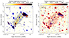 |
Fig. 3. Left: uGMRT band 4 image in color and in contours. The beam is 9.6″ × 3.8″ and the position angle is 7.5°. Right: uGMRT band 5 image in color and in contours (blue shows positive and gray shows negative contours). The beam is 6.1″ × 2.4″ and the position angle is −0.81°. The contour levels in both panels are −0.04, 0.04, 0.08, 0.16, etc. mJy beam−1. The MeerKAT 1.28 GHz image (Knowles et al. 2022) with a resolution of 7.2″ × 6.6″ and a position angle of 44.6° is overlaid in red contours at levels of 15, 30, 60, etc. μJy beam−1. The rms in the MeerKAT image is 5 μJy beam−1. |
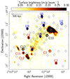 |
Fig. 4. uGMRT band-4 image in color. The discrete sources are marked as circles and are labeled. The diamonds show the positions of the spectroscopically identified cluster members by Sifón et al. (2013). The source labels from L14 are shown, and two new labels C12 and C13 are added. The prefix U refers to sources that are unrelated to the cluster, and sources with the prefix C are cluster members. |
Properties of the discrete radio sources in the cluster field.
4.2. Integrated spectra of the diffuse components
The radio relics and the halo likely have structures on angular scales that are smaller than the resolution. The comparison of the images at bands 3, 4, and 5 reveals structures within the relic and radio halo even at the highest-resolution images at band 5. At the redshift of El Gordo, the beam of 10″ corresponds to 78 kpc, which is in the range in which the relics and the halo can emit. A subtraction of point sources using uv-range cutoff would therefore subtract the features in the halo and the relics. The flux densities of the diffuse emission were measured from the robust 0 images convolved to a common resolution of 16″ resolution in the matched regions (Figure A.1). The flux densities of the discrete sources measured in robust 0 images made with an uv-range cutoff (> 3.4 kλ) were then subtracted from them. The E relic flux density for the part that was reported in L14 and the extension detected in the band 3 and 4 images are given separately. The flux densities and spectral indices obtained from power-law fits are reported in Table 3. The emission from the SE relic is well fit with a single power law, but with a marginal steepening. The integrated spectra and the power-law fits are shown in Figure 5. The k-corrected radio power of the radio halo at 1.4 GHz is (3.20 ± 0.20)×1025 W Hz−1. The largest linear sizes of the diffuse sources measured at band 3 are reported in Table 3. We compared the band 5 flux densities (discrete sources and diffuse emission) with those in the MeerKAT 1.28 GHz image and found them to be consistent within 1σ uncertainties. A study with a matched uv-coverage and without the discrete sources at uGMRT bands 3 and 4 and MeerKAT 1.28 GHz will be undertaken in the future.
Flux densities of the diffuse sources in El Gordo.
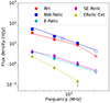 |
Fig. 5. Integrated spectra of the diffuse sources in El Gordo. The open symbols show the points from L14. The solid lines show the power-law fits. The spectral indices are reported in Table 3. The dashed lines join the points for the respective diffuse components that were not included in the fits. |
4.3. Spectral index map
We created a spectral index map using band 3 and 4 observations, in which the maximum extent of the radio halo was detected at both frequencies. We used a uv-range cut of > 3.4 kλ to image the contribution from the discrete sources. The mask was manually created to avoid the part of the NW relic that contains structure even at the scales of discrete sources. The discrete-source model was subtracted from the uv-data, and the residual visibilities were imaged using uniform weights in the uv-range of 0.065 − 12 kλ at both the bands. The images were convolved to the highest possible common circular resolution of 15″ × 15″. They were then combined to create the spectral index map and the corresponding error map shown in Figure 6. We masked the pixels below 3σrms from each image. This helped us to avoid regions with large errors on the spectral index.
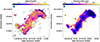 |
Fig. 6. Left: Spectral index map between 366 MHz and 672 MHz for the radio halo in El-Gordo at 15″ × 15″ resolution in color scale. The contours from the 672 MHz image at 0.1, 0.2, 0.4, 0.8, and 1.6 mJy beam−1 are overlaid. Right: Spectral index error map. High errors at the edges are expected due to the low S/N at the outskirts. The numbered regions used for analysis are shown in the map. The beam is shown in the top left corner in both panels. |
The spectral index trend from north to south within the radio halo was analyzed in the numbered regions marked in the right panel of Figure 6. Figure 7 shows the trend of the spectral index over the regions. While the spectral indices in the northern part reach values < − 1.5, the southern region is flatter than −1.2. The NW relic shows an overall steep-to-flat spectral index trend from the outer to the inner edge. There is marginal evidence of a steepening in the spectral indices in the SE relic. Near the E relic, the spectra show a flatter outer edge, and there is marginal evidence for a steepening. The resolution of the map is not sufficient to resolve the spectral index across the E-relic and for the extension.
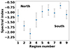 |
Fig. 7. Spectral indices with error bars obtained from the spectral index map plotted as a function of the numbered regions shown in the right panel of Fig. 6. |
4.4. Radio and X-ray point-to-point analysis
The morphology of radio halos generally follows that of the X-ray emission. This suggests an interplay between thermal and nonthermal components in the ICM (e.g., Govoni et al. 2001a; Giacintucci et al. 2005; Cova et al. 2019; Xie et al. 2020; Rajpurohit et al. 2021b; Balboni et al. 2024). This can also be observed in El Gordo, where the radio and X-ray emission are both elongated in the NW-SE direction (together with the relics). This indicates the main merger axis (Figure 1). To investigate the connection between thermal and nonthermal components more quantitatively, we used the Chandra and uGMRT data to compare the X-ray and radio surface brightnesses on a point-to-point basis (e.g., Govoni et al. 2001a).
As the first step of the analysis, we constructed a grid that covered the cluster. Each element of the grid was constituted by a square cell with a width of 9 pixels (1 pixel = 2″). This is broader than the synthesized beam (15″) of the radio image. We then measured the X-ray surface brightness in each cell from the Chandra point-source-subtracted image and the radio surface brightness from the band 3 and band 4 images that were used to produce the spectral index map. As we are interested in the radio halo emission, we excluded the cells located in the directions of the two relics from the analysis. The grid we obtained in this way is shown in Figure B.1 (in Appendix B).
In the second step, we plotted the radio and X-ray surface brightnesses in the IR − IX plots (Figure 8) to search for possible correlations between the two quantities. Generally, a power-law relation of the form
was used to fit the data, where the slope of the scaling (b) determined whether the radio brightness decreased more slowly than the X-ray brightness (if b < 1) or vice versa (if b > 1). We restricted the analysis and fitting to the data points for which the radio surface brightness was > 3σ, and we considered as upper limits (cyan arrows in Figure 8) the values below this threshold, following Botteon et al. (2020b) (see also Bonafede et al. 2021; Rajpurohit et al. 2021b). This cut on the y-axis required the use of a Bayesian linear regression method to take the selection effect into account. Therefore, we adopted the linmix package (Kelly 2007), which can handle censored data, to perform linear regression. The best-fit slopes for the band 3 and band 4 data are b = 0.60 ± 0.12 and b = 0.76 ± 0.12, respectively, suggesting that the magnetic field strength and relativistic particle density (traced by IR) declines more slowly than the thermal gas density (traced by IX). The obtained slopes agree with what is seen for the giant radio halos (e.g., Rajpurohit et al. 2023; Balboni et al. 2024; Santra et al. 2024a). The indication of an increase in b with frequency might be due to spectral steepening in fainter portions (outskirts) in X-rays. The strength and monotonic behavior of the relation was measured using the Pearson and Spearman correlation coefficients for the band 3 and band 4 data, which are rp = 0.54 and rs = 0.47, and rp = 0.64 and rs = 0.56, respectively.
 |
Fig. 8. Left: Radio surface brightness (IR) vs. X-ray surface brightness (IX) for band 3. The points in these plots are from the grid shown in Figure B.1. The cyan points are from the northern X-ray tail, the red points are from the southern X-ray tail, and the remaining points are from the rest of the halo. The fit to the points is shown as a solid black line, and the 95% confidence region is shown in the shaded part. The dashed red line shows the 1σ level of the radio images. The light blue arrows indicate the upper limits above 2σrms points. Right:IR vs. IX scaling plot for band 4 in the same color-code as in the left panel. |
A comparison of the spectral index distribution over the radio halo and the distribution of the X-ray surface brightness was made to confirm any correlation. For this purpose, a point-to-point comparison of the spectral index and X-ray surface brightness was carried out. The same grid as shown in Figure 9 was used, but only the cells in which the surface brightness in bands 3 and 4 exceeded 2σ were used (34 cells). The scatter found in the spectral index (α) and X-ray surface brightness (IX) was investigated for a correlation. Pearson and Spearman correlation coefficients of −0.58 and −0.57, respectively, were found. With the linmix package, the slope of the fitted line was found to be −0.57 ± 0.18. The spectral index and X-ray surface brightness are anticorrelated, which implies that the fainter parts in X-rays have steeper spectral indices and that the spectrum steepens radially outward.
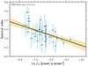 |
Fig. 9. Spectral index (α)-X-ray surface brightness point-to-point comparison (filled blue circles). The error bars are statistical measurement errors. The best fit is shown with the solid black line, and the confidence interval is shown as the shaded region. |
4.5. Comparison with the X-ray temperature, pressure, and entropy
We also compared the distribution of the diffuse radio emission with the X-ray temperature (Figure 10). The temperature of the two X-ray tails is very high. It peaks at 17.8 keV for the N tail and at 14.7 keV for the S tail, as measured from the spectral bins along the two tails depicted in the top left panel of Figure 10. We note, however, that due to the very low effective area of Chandra at high energy, the measurement of temperatures > 10 keV is critical, and it is impossible to confidently separate the temperature differences between adjacent hot bins or between the two tails, while the error from the spectral fitting does not entirely reflect the real uncertainty range for the same reason. Nevertheless, the X-ray thermodynamic properties show a possible trend along the elongation of the X-ray surface brightness from southeast to northwest. The pressure is higher and the entropy is lower in the southeast, and vice versa in the northwest. The radio halo emission is cospatial with the region that shows this trend (Figure 10).
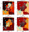 |
Fig. 10. Top left: X-ray temperature map in color. The dashed blue lines indicate the two X-ray tails that were shown in Fig. 1. Top right: Color map of the percentage error on the temperature (kT). The errors are dominated by the uncertainty on the temperature determination, which is ∼5% in the core region and ∼10% in the rest of the cluster. For the larger bins in the map, the temperature is not constrained. Bottom left: Pseudo-pressure map in logarithmic units in color. Bottom right: Entropy (K) map in color. The 672 MHz contours (cyan) from Figure 3 are overlaid in all the panels. |
4.6. Radio halo and the density fluctuation power spectrum
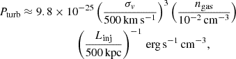
The power spectrum of the density fluctuations derived using X-ray images can be used as a tracer of turbulent motions in the ICM (e.g, Churazov et al. 2012; Gaspari & Churazov 2013; Zhuravleva et al. 2015; Zhang et al. 2023; Dupourqué et al. 2024). Based on the amplitude of density fluctuations at fixed spatial scales as a proxy for the level of turbulence, a scaling relation between the radio halo power and the velocity dispersion was found (Eckert et al. 2017). We applied a similar analysis as was performed by Eckert et al. (2017) to the Chandra data of El Gordo. After masking the bright bullet structure around the X-ray peak (see Figure 1), we used a principal component analysis to determine the position of the centroid of the cluster and its ellipticity. We then extracted a surface brightness profile in elliptical annuli around the X-ray centroid, which we fit in pyproffit (Eckert et al. 2020) with a single beta model (Cavaliere & Fusco-Femiano 1976). From the best-fit brightness profile, we created a 2D elliptical model image that accounted for CCD gaps and vignetting variations. The fluctuations at the top of the model image were computed by dividing the true image by the model and filtering the residual image with 2D Mexican hat functions, following the modified delta-variance method introduced by Arévalo et al. (2012). The 2D power at a given scale is then proportional to the variance of the Mexican hat filtered map. The 2D power spectrum of El Gordo within a circular region of 1 Mpc surrounding the X-ray centroid is shown in the left panel of Figure 11, where we compare the resulting power spectrum with the contribution of Poisson noise.
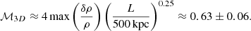
Numerical simulations of galaxy clusters showed that the turbulent Mach number ℳ = σv/cs is linearly related to the maximum amplitude of gas density fluctuations,  (Gaspari et al. 2014; Zhuravleva et al. 2014), where σv, cs are the velocity dispersion of the turbulent motion and the sound speed of the medium. To deproject the measured 2D power spectra and estimate the turbulent Mach number, we used the best-fit beta model to simulate a 3D galaxy cluster with properties similar to El Gordo, and we modified the 3D gas density field by a random 3D fluctuation field following a Kolmogorov power spectrum (it assumed a single injection scale). The perturbed 3D density field was then transformed into X-ray surface brightness and projected onto the line of sight to create a corresponding 2D surface brightness image. The ratio of the 2D to 3D power spectra in the simulated data was then used to convert the 2D power spectrum into a 3D power spectrum. This is shown as the green curve in the left panel of Figure 11. The 3D fractional amplitude of gas density fluctuations can then be retrieved as
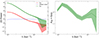 |
Fig. 11. Left: Fluctuation power spectrum in the central 1 Mpc of El Gordo, where the bullet is masked, as a function of wave number k. The red curve shows the 2D fluctuations in the power spectrum subtracted from the Poisson noise (blue curve). The green curve shows the corresponding deprojected 3D power spectrum. Right: Amplitude of 3D fluctuations |

with k the wave number, and P3D(k) the deprojected power spectrum. In the right panel of Figure 11, we show the retrieved amplitude of the gas density fluctuations in El Gordo as a function of wave number. The fluctuations peak at L = k−1 ≈ 700 kpc at an amplitude max(δρ/ρ) = 0.15 ± 0.02. The approximate relation between the density fluctuation amplitude and the turbulent Mach number reads (Gaspari et al. 2014)
For the ICM in El Gordo with kT ∼ 14 keV, the sound speed in the medium is cs = (γkT/μmp)1/2 ∼ 1915 km s−1, such that the velocity dispersion of turbulent motions can be estimated as σv = 1201 ± 88 km s−1.
We caution that the analysis presented here assumes that all the fluctuations in El Gordo should be attributed to turbulence. Although we masked the regions surrounding the bullet structure, inside which the fluctuations can be ascribed to a moving subhalo, additional sources of fluctuations in addition to intracluster turbulence might remian. As for most complex merging clusters, the value retrieved here should therefore be viewed as the maximum allowed value for the turbulent velocity dispersion.
4.7. Radio halo power and cluster mass
The scaling relation between cluster masses and the radio power of radio halos and relics can be used to infer the connection between the nonthermal and thermal components of the ICM (Basu 2012; Cassano et al. 2013; Cuciti et al. 2023). We plot the 1.4 GHz radio power of El Gordo in the P1.4 GHz − M500 plane along with other samples from the literature (Figure 12). The L14 1.4 GHz value for El Gordo that was extrapolated from their 2.1 GHz measurement is also plotted for comparison. The current measurement and that of L14 are consistent within the uncertainties. El Gordo is the most radio-luminous of the high-redshift samples (Di Gennaro et al. 2021a; Sikhosana et al. 2024). It is also the most massive of the high-redshift sample, and the radio power agrees with the expectation from the scaling relation. The radio powers for low-redshift clusters, reported at 150 MHz by Botteon et al. (2022) and at 947 MHz by Duchesne et al. (2024), were extrapolated to 1.4 GHz using a spectral index of −1.3. This is also shown in the same plot.
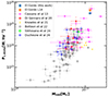 |
Fig. 12. 1.4 GHz radio power vs. mass (M500) plotted for El Gordo (this work and L14) with other samples of radio halos from the literature. The Di Gennaro et al. (2021a) sample consists of halos at redshifts > 0.6, the Knowles et al. (2021) contains radio halos in the redshift range of 0.22 < z < 0.65 and the local redshift (z ∼ 0.2) sample from Cassano et al. (2013). The recent discovery of the radio halo in ACT-CL J0329.2-2330 (z = 1.23) is also shown (Sikhosana et al. 2024). The large samples from the LOFAR survey by Botteon et al. (2022) (0.016 < z < 0.9), and from ASKAP by Duchesne et al. (2024) (0.01 < z < 0.5) have been added to provide a more comprehensive picture. |
5. Discussion
El Gordo is a high-redshift powerful radio halo with a double relic system. The recent high-redshift sample presented by Di Gennaro et al. (2021a) contains only one relic in PSZ2 G091.83+26.11 at z = 0.822. A further candidate relic at high redshift was reported in PSZ2 G069.39+68.05 (z = 0.762) by Botteon et al. 2022. This makes El Gordo the only cluster so far with a double radio relic system and a radio halo known at redshift > 0.6. It is a peculiar system also in the X-ray band, where it shows a comet-like morphology with two tails. We presented the images and spatially resolved spectra of the radio halo and the relics using the uGMRT between 300–1450 MHz. We detected the radio relics and the halo, which were known earlier. We also found fainter extensions of them. The eastern relic extends farther north to a total extent of 1030 kpc (134″). This feature is tentatively also detected at band 4, but not at band 5 (Figure 3). The NW relic is found to have the same spatial and spectral features as found by L14, and the integrated spectrum is a power-law with a spectral index of −1.3 ± 0.4. The physical picture of the origin of the radio relic in a shock of Mach number ≳3 presented in Botteon et al. (2016) therefore still holds.
The radio halo is cospatial with the X-ray emission, as reported earlier, but the emission also extends over the southern tail (Figure 1). In the 610 MHz image using the legacy GMRT, it was clear that the radio halo preferred the northern X-ray tail. In deeper low-frequency observations at 366 MHz, the fainter parts of the radio halo that also extend over the southern X-ray tail are detected (Figure 1). The integrated spectrum of the radio halo in El Gordo is a power law with a spectral index −1.0 ± 0.3 in the frequency range of 366–1274 MHz. However, between 1274 and 2100 MHz, a steepening to −2.50 ± 0.46 is observed (Figure 5). Curved radio spectra in radio halos were only found in handful of clusters, such as Coma (Thierbach et al. 2003; Murgia et al. 2024), AS1063 (Xie et al. 2020), MACSJ0717.5+3745 (Rajpurohit et al. 2021a), and A3562 (Venturi et al. 2022). We emphasize that the 2100 MHz flux measurements may be biased due to the different uv-coverage, and the different regions were also used to estimate the flux density. More sensitive observations at 2000 MHz and measurements with a matched uv range can shed light on the robustness of the steepening, however.
The origin of radio halos was proposed to be a turbulent reacceleration process (e.g., Brunetti et al. 2001, 2007; Petrosian 2001; Cassano & Brunetti 2005; Brunetti & Lazarian 2011, 2016; Miniati 2015; Nishiwaki & Asano 2022). This stochastic process reaccelerates a mildly relativistic population of electrons. Hadronic collisions are present in the ICM and produce relativistic electrons, but it was shown in many cases that they are not sufficient to explain radio halos and the constraints from gamma rays (e.g., Brunetti et al. 2008, 2017; Wilber et al. 2018; Adam et al. 2021; Bruno et al. 2021; Di Gennaro et al. 2021a; Osinga et al. 2024; Pasini et al. 2024; Nishiwaki & Asano 2025). Turbulence and shocks are known to be injected during cluster mergers, as shown by simulations and also observed in a number of clusters (e.g., Miniati et al. 2000; Miniati 2015; Vazza et al. 2017).
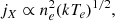
We used a point-to-point comparison of the radio and X-ray images as a tool to test the theoretical models (Govoni et al. 2001a). The rationale behind the tool is that the gravitational potential energy from cluster mergers will dissipate as shocks and turbulence in the ICM: A fraction goes into the amplification of the magnetic field and into particle acceleration. Under the assumption that the fraction of energy that is channeled into nonthermal components is independent of the position in the cluster, predictions for the radio-Xray surface brightness scaling can be obtained. The bolometric X-ray emissivity (jX) is given by
where ne is electron density, and kTe is the temperature. The thermal energy density (ϵth ∝ 3neKTe) squared equals the emissivity at a given position if the cluster is isothermal, resulting in
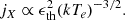
For the relativistic electrons, the number density between energies ϵ and ϵ + dϵ can be assumed to be N(ϵ)dϵN0ϵ−δdϵ. The radio emissivity is then given by

where B is the magnetic field. For a linear relation between thermal and nonthermal plasma, it is expected that
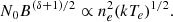
Under the assumption that the cosmic-ray proton energy density (ϵCRp) and magnetic field (ϵB = B2/8π) energy density is proportional to the thermal energy density (ϵCRp ∝ ϵth and ϵB = ϵth), the scaling relation for hadronic models is expected to be linear in the case of strong magnetic fields (as compared to the equivalent magnetic field for the CMB) and superlinear in weak magnetic fields, assuming a radially decreasing magnetic field strength in the cluster. Supe-linear scaling has been found in mini-halos (e.g. Ignesti et al. 2020, 2022; Riseley et al. 2023; Lusetti et al. 2024; Biava et al. 2024). The turbulent reacceleration can generate different slopes from super- to sublinear or linear, depending on the parameters for the faint radio halos. If the electrons (energy density) and the magnetic fields (energy density) follow the thermal energy density, the models in the case of isothermal distribution and constant turbulent Mach number produce a slope that is sublinear to linear (from strong to weak field) (see Eq. (12) Balboni et al. 2024), as seen in the clusters A 2744 and A2255 (Govoni et al. 2001b; Botteon et al. 2020b) and for the 3 GHz scaling relation for the radio halo in MACS0717.5+3745 (Rajpurohit et al. 2021a).
For El Gordo, we found the relations to be sublinear (0.60 ± 0.12 at band 3 and 0.76 ± 0.12 at band 4). Di Gennaro et al. (2023) reported a linear to superlinear correlation slope from 0.14–3.0 GHz for PSZ2 G091.83+26.11 at a redshift of 0.822. Other radio halos such as Coma (Govoni et al. 2001b; Bonafede et al. 2022), A520 (Hoang et al. 2019), MACS J1149.5+2223 (Bruno et al. 2021), and AS1063 (Xie et al. 2020) have sublinear correlations. For MACS J0717.5+3745 at 144 and 1500 MHz (Rajpurohit et al. 2021a), the correlations are sublinear but approach linear at higher frequencies. In El Gordo, the band 4 (672 MHz) correlation slope is also marginally higher than that at 366 MHz, but no firm trend can be established given the uncertainties. This steeping can be attributed to the spectral steepening (the radial decay of the nonthermal plasma is different in frequency) of the radio halo. Moreover, the SZ decrement at this high redshift can play a role in the steepening. Further study using MeerKAT data at 1.28 GHz and other higher-frequency observations (above 1.5 GHz) are needed to confirm this.
The arguments regarding the expected correlation slopes employ several assumptions, such as isothermality of the cluster and that the fraction of energy that goes into the nonthermal components is independent of the position in the cluster. The thermodynamic maps of El Gordo show that the properties varies considerably in the cluster (Figure 10). The southern part of the radio halo, cospatial with the X-ray core, has lower temperatures (6 − 8 keV) and a higher pseudo-pressure, and the northern part has higher temperatures and a lower pseudo-pressure. We also tried to investigate whether the parts of the radio halo along the two X-ray tails behave differently in the IR − IX correlation but the current data limited us to only a few points (Figure 8). It was therefore not possible to find any trend. Future work combining MeerKAT data with deeper uGMRT observations might make this possible.
The spectral index is anticorrelated with the X-ray surface brightness with a slope of −0.57 ± 0.18 and a correlation coefficient of −0.58. To date, studies of the correlation between the spectral index and the X-ray surface brightness were made for a handful of halos, such as A2255 (Botteon et al. 2020b) and MACSJ0717.5+3745 (Rajpurohit et al. 2021b), A2256 (Rajpurohit et al. 2023), A521 (Santra et al. 2024b), and A2142 (Riseley et al. 2024). An observed anticorrelation suggests a spectral steepening in the outermost regions of the halo, indicating that the faint X-ray emission probes the steep spectrum regions in the cluster outskirts. Since the radio halo is not circularly symmetric, a radial profile analysis will be hard. However, this trend, along with the increasing correlation slope, implies a spectral steepening in the outskirts, similar to what was seen in L.14.
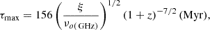
Using the X-ray fluctuation power spectrum approach described in Sect. 4.6, Eckert et al. (2017) derived an empirical scaling relation between the radio power of radio halos (P1.4 GHz) and the three-dimensional turbulent velocity dispersion (σv),

with  ,
,  , with an intrinsic scatter
  . Given the total radio power of the radio halo in El Gordo, the scaling relation predicts σv of 1112
 km s−1 (estimated using the error propagation). This value is close to and consistent with the value σv = 1, 201 ± 88 km s−1 estimated from the amplitude of fluctuations in the ICM of El Gordo (see Sect. 4.6). Direct measurements of these motions will be available in future observations with X-Ray Imaging and Spectroscopy Mission (XRISM). The Equation (8) is an empirical relation and is based on low-z radio halos. The obtained velocity dispersion can therefore be considered as the lower limit. The X-ray and radio properties of the radio halo in El Gordo are consistent with the properties extracted from the GMRT radio halo sample (Eckert et al. 2017). The very high-velocity dispersion and radio power place the system at the high-power end of the relation. Only MACS J0717.5+3745 and the Bullet cluster (radio powers of (52.48 ± 20.56) × 1024, (23.44 ± 1.51) × 1024 W Hz−1, and velocity dispersions of 1206 ± 96, 977 ± 99 km s−1, respectively) exhibit similarly high values for the turbulent velocity and radio power.
The energy rate per unit volume related to turbulence can be estimated as (Eq. (2) Eckert et al. 2017),
where Linj is the injection scale, and ngas is the thermal gas density. For Linj of 500 kpc, we estimate Pturb to be 1.07 × 10⁻²⁵ erg s−1 cm−3. Simulations proposed impact parameters of 300 kpc (Molnar & Broadhurst 2015) and 800 kpc (Zhang et al. 2015) for mergers that match the features of El Gordo. Using 800 and 300 kpc (assuming the scale of injection to be similar to the impact parameter) as the injection scales, we obtain Pturb = 6.74 × 10⁻²⁶ and 1.79 × 10⁻²⁵ erg s−1 cm−3, respectively.
The reacceleration mechanism that generated the relativistic electrons in the radio halo has to work at a rate that balances the radiative losses over long timescales, and τmax is the maximum lifetime of the electrons that must be balanced by reacceleration, given by (Eq. (14), Brunetti & Lazarian 2016)
where νo( GHz) is the observing frequency, and ξ is a factor in the range 6–8 (we used a value of 7), such that the steepening frequency νs ∼ ξνb, where νb is the critical synchrotron frequency emitted by electrons with the same acceleration time as their radiative lifetime (Cassano & Brunetti 2005). The magnetic field considered is given by  (the condition for the maximum radiative lifetime). The observed frequency is νo = νs/(1 + z). The steepening frequency for the radio halo in El Gordo is likely to be between 1.274 and 2.1 GHz (Figure 5). Assuming steepening frequencies of 1.274 GHz and 2.1 GHz, we find τmax to be 41 Myr, and 31 Myr, respectively. This timescale for the Coma cluster is ∼400 Myr (e.g., Brunetti & Lazarian 2016). Thus, at the high redshift of El Gordo, the maximum available acceleration time is shorter by a factor of 10. The available acceleration timescale τacc has to be shorter than τmax.
When we assume transit-time-damping (TTD) in the collisional regime, a reference model for radio halos (e.g., Brunetti et al. 2007), the acceleration time is ∼70–80 Myr (using the Mach number, sound speed, and injection scale). This is very close to what was obtained using Equation (10). However, it should be noted that the τmax and the turbulent Mach numbers are upper limits, and the efficiency needed for the acceleration might therefore be higher. This might suggest a situation in which the effective mfp of the ICM particles is lower than that due to Coulomb collisions. In this situation, the acceleration time is shorter and the acceleration efficiency is higher (e.g., Brunetti & Lazarian 2011). There is possible evidence for a reduced mean free path in the ICM (e.g., Zhuravleva et al. 2019; Di Gennaro et al. 2021a). When we assume the nonresonant acceleration proposed in Brunetti & Lazarian (2016), the reacceleration timescale is τacc ∼ 450(ψ/0.5)0.3 (Myr), (where ψ = lmfp/lA, and lmfp, lA are the mean free path and Alfvén scale, respectively), implies a constraint on the mean free path of the relativistic electrons to ≤0.3, hence lmfp ≤ lA. This is slightly lower than the reference value (∼0.5) that was motivated and used in previous studies (e.g., Brunetti & Lazarian 2016; Brunetti & Vazza 2020). Therefore, these extreme conditions may be used to check models and start suggesting that the efficiency constrained by observations is slightly higher than that expected by models in the standard or original configuration of the model parameters.
6. Summary and conclusions
We have presented a study of the high-redshift galaxy cluster El Gordo at 300–1450 MHz using the uGMRT. The sensitive uGMRT observations allowed us to study the detailed spectral characteristics of the radio halo below 1 GHz for the first time. Our observations, combined with available X-ray observations (Chandra), provided acute physical insights into the thermal and nonthermal connections in the ICM and into the origin of the radio halo. We summarize our results and conclusions below.
-
We obtained GMRT images of El Gordo at the effective frequencies of 366, 672, and 1274 MHz with an rms noise of 50, 13 and 15 μJy beam−1. We detected the radio halo, the NW relic, SE relic, and E relic, which were known from earlier studies. In addition, we detected an extension of the E relic to the north, which we labeled E-relic ext.
-
The radio halo emission is well fit with a single power law between 300–1274 MHz, with a spectral index of −1.0 ± 0.3. The 2.1 GHz measurement from L14 indicates a steepening beyond 1274 MHz with a spectral index of −2.50 ± 0.46. The differences in the uv-coverage might affect this estimate, however. The integrated spectral indices of the NW relic, SE relic, and E relic were also fit with a single power law with a slope of −1.4. The E relic ext has a steep spectrum of −2.1. The radio power of the halo at 1.4 GHz follows the P1.4 GHz versus M500 relation for high-redshift halos and is the second brightest radio halo of all the radio halos at all redshifts.
-
We obtained a spectral index map between 366 and 672 MHz that showed that the radio halo has a median spectral index of −1.3, and it shows a standard deviation of 0.4. However, the southern part shows flatter spectral indices (> − 1.0) than the northern part, where the spectral indices reach steeper values (< − 2). This suggests a more complex situation than a simple power law. The NW relic also shows a gradient of the spectral index from the outer to the inner edge.
-
The brighter portion of the radio halo follows the northern X-ray tail. The Chandra temperature measurements at the edges of the radio emission are not robust enough to conclude about the cospatiality with higher-temperature regions and the brighter radio emission.
-
The point-to-point comparison of 366 and 672 MHz images with the X-ray surface brightness showed sublinear fits, but with scatter at low surface brightness values. The relation was examined separately for the northern and southern X-ray tails. Both regions lie within the range in which in the scaling relation is strongly scattered, and the southern tail has only three points. The point-to-point comparison of the spectral index with the X-ray surface brightness showed that they are anticorrelated, indicating that the brighter portions in X-ray have flatter spectra and vice versa.
-
Using the radio power of the halo, we calculated the turbulent velocity dispersion based on the scaling by Eckert et al. (2017) to be 1112 km s−1, implying a 3D turbulent Mach number of ∼0.6. The power spectrum of X-ray surface brightness fluctuations in the cluster provides a consistent estimate of the turbulent Mach number. Further assuming the turbulence injection scale to be the same as the cluster merger impact parameters proposed in simulations, we found the energy rate per unit volume of turbulence, Pturb to be 1.79 × 10⁻²⁵ and 6.74 × 10⁻²⁶ erg s−1 cm−3, if the typical scale of injection of turbulence is in the range 300–800 kpc.
Acknowledgments
The authors thank the referees for their comments that improved the paper. R.K. and R.S. acknowledge the support of the Department of Atomic Energy, Government of India, under project no. 12-R&D-TFR-5.02-0700. R.K. also acknowledges the support from the SERB Women Excellence Award WEA/2021/000008. We thank the staff of the GMRT that made these observations possible. GMRT is run by the National Centre for Radio Astrophysics of the Tata Institute of Fundamental Research. This research has made use of the data from the GMRT Archive. This research has made use of data obtained through the High Energy Astrophysics Science Archive Research Center Online Service, provided by the NASA/Goddard Space Flight Center. This research has made use of NASA’s Astrophysics Data System, and of the NASA/IPAC Extragalactic Database (NED) which is operated by the Jet Propulsion Laboratory, California Institute of Technology, under contract with the National Aeronautics and Space Administration. The MeerKAT telescope is operated by the South African Radio Astronomy Observatory, which is a facility of the National Research Foundation, an agency of the Department of Science and Innovation. This research has made use of data obtained from the Chandra Data Archive provided by the Chandra X-ray Center (CXC).
References
- Adam, R., Goksu, H., Brown, S., Rudnick, L., & Ferrari, C. 2021, A&A, 648, A60 [NASA ADS] [CrossRef] [EDP Sciences] [Google Scholar]
- Arévalo, P., Churazov, E., Zhuravleva, I., Hernández-Monteagudo, C., & Revnivtsev, M. 2012, MNRAS, 426, 1793 [CrossRef] [Google Scholar]
- Arnaud, K. A. 1996, in Astronomical Data Analysis Software and Systems V, eds. G. H. Jacoby, & J. Barnes, ASP Conf. Ser., 101, 17 [NASA ADS] [Google Scholar]
- Balboni, M., Gastaldello, F., Bonafede, A., et al. 2024, A&A, 686, A5 [NASA ADS] [CrossRef] [EDP Sciences] [Google Scholar]
- Basu, K. 2012, MNRAS, 421, L112 [Google Scholar]
- Biava, N., Bonafede, A., Gastaldello, F., et al. 2024, A&A, 686, A82 [NASA ADS] [CrossRef] [EDP Sciences] [Google Scholar]
- Bonafede, A., Intema, H. T., Brüggen, M., et al. 2014, MNRAS, 444, L44 [Google Scholar]
- Bonafede, A., Brunetti, G., Vazza, F., et al. 2021, ApJ, 907, 32 [Google Scholar]
- Bonafede, A., Brunetti, G., Rudnick, L., et al. 2022, ApJ, 933, 218 [NASA ADS] [CrossRef] [Google Scholar]
- Botteon, A., Gastaldello, F., Brunetti, G., & Kale, R. 2016, MNRAS, 463, 1534 [Google Scholar]
- Botteon, A., Gastaldello, F., & Brunetti, G. 2018, MNRAS, 476, 5591 [Google Scholar]
- Botteon, A., Brunetti, G., Ryu, D., & Roh, S. 2020a, A&A, 634, A64 [NASA ADS] [CrossRef] [EDP Sciences] [Google Scholar]
- Botteon, A., Brunetti, G., van Weeren, R. J., et al. 2020b, ApJ, 897, 93 [Google Scholar]
- Botteon, A., Shimwell, T. W., Cassano, R., et al. 2022, A&A, 660, A78 [NASA ADS] [CrossRef] [EDP Sciences] [Google Scholar]
- Brunetti, G. 2011, MMSAI, 82, 515 [Google Scholar]
- Brunetti, G., & Jones, T. W. 2014, IJMPD, 23, 30007 [Google Scholar]
- Brunetti, G., & Lazarian, A. 2011, MNRAS, 410, 127 [Google Scholar]
- Brunetti, G., & Lazarian, A. 2016, MNRAS, 458, 2584 [Google Scholar]
- Brunetti, G., & Vazza, F. 2020, Phys. Rev. Lett., 124, 30007 [Google Scholar]
- Brunetti, G., Setti, G., Feretti, L., & Giovannini, G. 2001, MNRAS, 320, 365 [Google Scholar]
- Brunetti, G., Venturi, T., Dallacasa, D., et al. 2007, ApJ, 670, L5 [Google Scholar]
- Brunetti, G., Giacintucci, S., Cassano, R., et al. 2008, Nature, 455, 944 [Google Scholar]
- Brunetti, G., Zimmer, S., & Zandanel, F. 2017, MNRAS, 472, 1506 [Google Scholar]
- Bruno, L., Rajpurohit, K., Brunetti, G., et al. 2021, A&A, 650, A44 [NASA ADS] [CrossRef] [EDP Sciences] [Google Scholar]
- Cassano, R., & Brunetti, G. 2005, MNRAS, 357, 1313 [Google Scholar]
- Cassano, R., Ettori, S., Giacintucci, S., et al. 2010, ApJ, 721, L82 [Google Scholar]
- Cassano, R., Ettori, S., Brunetti, G., et al. 2013, ApJ, 777, 141 [Google Scholar]
- Cassano, R., Botteon, A., Di Gennaro, G., et al. 2019, ApJ, 881, L18 [Google Scholar]
- Cavaliere, A., & Fusco-Femiano, R. 1976, A&A, 500, 95 [NASA ADS] [Google Scholar]
- Chandra, P., & Kanekar, N. 2017, ApJ, 846, 111 [Google Scholar]
- Churazov, E., Vikhlinin, A., Zhuravleva, I., et al. 2012, MNRAS, 421, 1123 [NASA ADS] [CrossRef] [Google Scholar]
- Cova, F., Gastaldello, F., Wik, D. R., et al. 2019, A&A, 628, A83 [NASA ADS] [CrossRef] [EDP Sciences] [Google Scholar]
- Cuciti, V., Cassano, R., Brunetti, G., et al. 2015, A&A, 580, A97 [CrossRef] [EDP Sciences] [Google Scholar]
- Cuciti, V., Cassano, R., Brunetti, G., et al. 2021, A&A, 647, A51 [EDP Sciences] [Google Scholar]
- Cuciti, V., Cassano, R., Sereno, M., et al. 2023, A&A, 680, A30 [NASA ADS] [CrossRef] [EDP Sciences] [Google Scholar]
- de Gasperin, F., Rudnick, L., Finoguenov, A., et al. 2022, A&A, 659, A146 [NASA ADS] [CrossRef] [EDP Sciences] [Google Scholar]
- Dennison, B. 1980, ApJ, 239, L93 [Google Scholar]
- Di Gennaro, G., van Weeren, R. J., Brunetti, G., et al. 2021a, Nat. Astron., 5, 268 [Google Scholar]
- Di Gennaro, G., van Weeren, R. J., Cassano, R., et al. 2021b, A&A, 654, A166 [NASA ADS] [CrossRef] [EDP Sciences] [Google Scholar]
- Di Gennaro, G., Brüggen, M., van Weeren, R. J., et al. 2023, A&A, 675, A51 [NASA ADS] [CrossRef] [EDP Sciences] [Google Scholar]
- Di Mascolo, L., Mroczkowski, T., Perrott, Y., et al. 2021, A&A, 650, A153 [NASA ADS] [CrossRef] [EDP Sciences] [Google Scholar]
- Dolag, K., & Enßlin, T. A. 2000, A&A, 362, 151 [NASA ADS] [Google Scholar]
- Donnert, J. M. F. 2014, MNRAS, 438, 1971 [NASA ADS] [CrossRef] [Google Scholar]
- Duchesne, S. W., Johnston-Hollitt, M., Offringa, A. R., et al. 2021, PASA, 38, e010 [NASA ADS] [CrossRef] [Google Scholar]
- Duchesne, S. W., Botteon, A., Koribalski, B. S., et al. 2024, PASA, 41, e026 [NASA ADS] [CrossRef] [Google Scholar]
- Dupourqué, S., Clerc, N., Pointecouteau, E., et al. 2024, A&A, 687, A58 [NASA ADS] [CrossRef] [EDP Sciences] [Google Scholar]
- Eckert, D., Gaspari, M., Vazza, F., et al. 2017, ApJ, 843, L29 [Google Scholar]
- Eckert, D., Finoguenov, A., Ghirardini, V., et al. 2020, Open J. Astrophys., 3, 12 [NASA ADS] [CrossRef] [Google Scholar]
- Enßlin, T. A., Biermann, P. L., Klein, U., & Kohle, S. 1998, A&A, 332, 395 [Google Scholar]
- Fujita, Y., Takizawa, M., Yamazaki, R., Akamatsu, H., & Ohno, H. 2015, ApJ, 815, 116 [NASA ADS] [CrossRef] [Google Scholar]
- Gaspari, M., & Churazov, E. 2013, A&A, 559, A78 [NASA ADS] [CrossRef] [EDP Sciences] [Google Scholar]
- Gaspari, M., Churazov, E., Nagai, D., Lau, E. T., & Zhuravleva, I. 2014, A&A, 569, A67 [NASA ADS] [CrossRef] [EDP Sciences] [Google Scholar]
- Giacintucci, S., Venturi, T., Brunetti, G., et al. 2005, A&A, 440, 867 [NASA ADS] [CrossRef] [EDP Sciences] [Google Scholar]
- Giacintucci, S., Venturi, T., Macario, G., et al. 2008, A&A, 486, 347 [NASA ADS] [CrossRef] [EDP Sciences] [Google Scholar]
- Govoni, F., Enßlin, T. A., Feretti, L., & Giovannini, G. 2001a, A&A, 369, 441 [NASA ADS] [CrossRef] [EDP Sciences] [Google Scholar]
- Govoni, F., Feretti, L., Giovannini, G., et al. 2001b, A&A, 376, 803 [CrossRef] [EDP Sciences] [Google Scholar]
- Hoang, D. N., Shimwell, T. W., van Weeren, R. J., et al. 2019, A&A, 622, A20 [NASA ADS] [CrossRef] [EDP Sciences] [Google Scholar]
- Hoeft, M., & Brüggen, M. 2007, MNRAS, 375, 77 [Google Scholar]
- Hu, Y., Stuardi, C., Lazarian, A., et al. 2024, Nat. Commun., 15, 1006 [NASA ADS] [CrossRef] [Google Scholar]
- Ignesti, A., Brunetti, G., Gitti, M., & Giacintucci, S. 2020, A&A, 640, A37 [NASA ADS] [CrossRef] [EDP Sciences] [Google Scholar]
- Ignesti, A., Brunetti, G., Shimwell, T., et al. 2022, A&A, 659, A20 [NASA ADS] [CrossRef] [EDP Sciences] [Google Scholar]
- Jee, M. J., Hughes, J. P., Menanteau, F., et al. 2014, ApJ, 785, 20 [NASA ADS] [CrossRef] [Google Scholar]
- Kale, R., & Ishwara-Chandra, C. H. 2021, Exp. Astron., 51, 95 [NASA ADS] [CrossRef] [Google Scholar]
- Kale, R., Dwarakanath, K. S., Bagchi, J., & Paul, S. 2012, MNRAS, 426, 1204 [NASA ADS] [CrossRef] [Google Scholar]
- Kale, R., Venturi, T., Giacintucci, S., et al. 2015, A&A, 579, A92 [NASA ADS] [CrossRef] [EDP Sciences] [Google Scholar]
- Kang, H., & Jones, T. W. 2005, ApJ, 620, 44 [NASA ADS] [CrossRef] [Google Scholar]
- Kang, H., & Ryu, D. 2011, ApJ, 734, 18 [Google Scholar]
- Kelly, B. C. 2007, ApJ, 665, 1489 [Google Scholar]
- Knowles, K., Pillay, D. S., Amodeo, S., et al. 2021, MNRAS, 504, 1749 [NASA ADS] [CrossRef] [Google Scholar]
- Knowles, K., Cotton, W. D., Rudnick, L., et al. 2022, A&A, 657, A56 [NASA ADS] [CrossRef] [EDP Sciences] [Google Scholar]
- Lindner, R. R., Baker, A. J., Hughes, J. P., et al. 2014, ApJ, 786, 49 [NASA ADS] [CrossRef] [Google Scholar]
- Lusetti, G., Bonafede, A., Lovisari, L., et al. 2024, A&A, 683, A132 [NASA ADS] [CrossRef] [EDP Sciences] [Google Scholar]
- Marriage, T. A., Acquaviva, V., Ade, P. A. R., et al. 2011, ApJ, 737, 61 [Google Scholar]
- Menanteau, F., González, J., Juin, J.-B., et al. 2010, ApJ, 723, 1523 [Google Scholar]
- Menanteau, F., Hughes, J. P., Sifón, C., et al. 2012, ApJ, 748, 7 [NASA ADS] [CrossRef] [Google Scholar]
- Miniati, F. 2015, ApJ, 800, 60 [Google Scholar]
- Miniati, F., Ryu, D., Kang, H., et al. 2000, ApJ, 542, 608 [NASA ADS] [CrossRef] [Google Scholar]
- Molnar, S. M., & Broadhurst, T. 2015, ApJ, 800, 37 [NASA ADS] [CrossRef] [Google Scholar]
- Murgia, M., Govoni, F., Vacca, V., et al. 2024, MNRAS, 528, 6470 [Google Scholar]
- Nishiwaki, K., & Asano, K. 2022, ApJ, 934, 182 [NASA ADS] [CrossRef] [Google Scholar]
- Nishiwaki, K., & Asano, K. 2025, ApJ, 978, 62 [Google Scholar]
- Osinga, E., van Weeren, R. J., Boxelaar, J. M., et al. 2021, A&A, 648, A11 [NASA ADS] [CrossRef] [EDP Sciences] [Google Scholar]
- Osinga, E., van Weeren, R. J., Brunetti, G., et al. 2024, A&A, 688, A175 [NASA ADS] [CrossRef] [EDP Sciences] [Google Scholar]
- Pasini, T., De Gasperin, F., Brüggen, M., et al. 2024, A&A, 689, A218 [NASA ADS] [CrossRef] [EDP Sciences] [Google Scholar]
- Perley, R. A., & Butler, B. J. 2017, ApJS, 230, 7 [NASA ADS] [CrossRef] [Google Scholar]
- Petrosian, V. 2001, ApJ, 557, 560 [Google Scholar]
- Pinzke, A., Oh, S. P., & Pfrommer, C. 2017, MNRAS, 465, 4800 [Google Scholar]
- Rajpurohit, K., Hoeft, M., van Weeren, R. J., et al. 2018, ApJ, 852, 65 [Google Scholar]
- Rajpurohit, K., Brunetti, G., Bonafede, A., et al. 2021a, A&A, 646, A135 [NASA ADS] [CrossRef] [EDP Sciences] [Google Scholar]
- Rajpurohit, K., Vazza, F., van Weeren, R. J., et al. 2021b, A&A, 654, A41 [NASA ADS] [CrossRef] [EDP Sciences] [Google Scholar]
- Rajpurohit, K., Osinga, E., Brienza, M., et al. 2023, A&A, 669, A1 [NASA ADS] [CrossRef] [EDP Sciences] [Google Scholar]
- Riseley, C. J., Biava, N., Lusetti, G., et al. 2023, MNRAS, 524, 6052 [NASA ADS] [CrossRef] [Google Scholar]
- Riseley, C. J., Bonafede, A., Bruno, L., et al. 2024, A&A, 686, A44 [NASA ADS] [CrossRef] [EDP Sciences] [Google Scholar]
- Rossetti, M., Ghizzardi, S., Molendi, S., & Finoguenov, A. 2007, A&A, 463, 839 [NASA ADS] [CrossRef] [EDP Sciences] [Google Scholar]
- Russell, H. R., McNamara, B. R., Sanders, J. S., et al. 2012, MNRAS, 423, 236 [NASA ADS] [CrossRef] [Google Scholar]
- Sanders, J. S. 2006, MNRAS, 371, 829 [Google Scholar]
- Santra, R., Kale, R., Giacintucci, S., et al. 2024a, ApJ, 976, 66 [Google Scholar]
- Santra, R., Kale, R., Giacintucci, S., et al. 2024b, ApJ, 962, 40 [NASA ADS] [CrossRef] [Google Scholar]
- Sifón, C., Menanteau, F., Hasselfield, M., et al. 2013, ApJ, 772, 25 [CrossRef] [Google Scholar]
- Sikhosana, S. P., Hilton, M., Bernardi, G., et al. 2024, A&A, submitted [arXiv:2404.03944] [Google Scholar]
- Sunyaev, R. A., & Zeldovich, Y. B. 1972, Comm. Astrophys. Space Phys., 4, 173 [Google Scholar]
- Thierbach, M., Klein, U., & Wielebinski, R. 2003, A&A, 397, 53 [NASA ADS] [CrossRef] [EDP Sciences] [Google Scholar]
- van Weeren, R. J., Röttgering, H. J. A., Brüggen, M., & Hoeft, M. 2010, Science, 330, 347 [Google Scholar]
- van Weeren, R. J., de Gasperin, F., Akamatsu, H., et al. 2019, Space Sci. Rev., 215, 16 [Google Scholar]
- Vazza, F., Jones, T. W., Brüggen, M., et al. 2017, MNRAS, 464, 210 [Google Scholar]
- Venturi, T., Giacintucci, S., Dallacasa, D., et al. 2008, A&A, 484, 327 [NASA ADS] [CrossRef] [EDP Sciences] [Google Scholar]
- Venturi, T., Giacintucci, S., Merluzzi, P., et al. 2022, A&A, 660, A81 [NASA ADS] [CrossRef] [EDP Sciences] [Google Scholar]
- Wilber, A., Brüggen, M., Bonafede, A., et al. 2018, MNRAS, 473, 3536 [Google Scholar]
- Wright, E. L. 2006, PASP, 118, 1711 [NASA ADS] [CrossRef] [Google Scholar]
- Xie, C., van Weeren, R. J., Lovisari, L., et al. 2020, A&A, 636, A3 [NASA ADS] [CrossRef] [EDP Sciences] [Google Scholar]
- Zhang, C., Yu, Q., & Lu, Y. 2015, ApJ, 813, 129 [NASA ADS] [CrossRef] [Google Scholar]
- Zhang, X., Simionescu, A., Gastaldello, F., et al. 2023, A&A, 672, A42 [NASA ADS] [CrossRef] [EDP Sciences] [Google Scholar]
- Zhuravleva, I., Churazov, E. M., Schekochihin, A. A., et al. 2014, ApJ, 788, L13 [Google Scholar]
- Zhuravleva, I., Churazov, E., Arévalo, P., et al. 2015, MNRAS, 450, 4184 [NASA ADS] [CrossRef] [Google Scholar]
- Zhuravleva, I., Churazov, E., Schekochihin, A. A., et al. 2019, Nat. Astron., 3, 832 [Google Scholar]
Appendix A: Regions used for flux density measurements
The regions used for the flux density measurements of the diffuse sources described in Sec. 4.2 are shown.
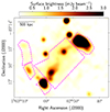 |
Fig. A.1. The uGMRT band 3 image with a resolution of 16″×16″ is shown in color with the regions used to measure the flux densities of the diffuse sources overlaid in dashed lines. |
Appendix B: Grids used for the point to point analysis
We show here the regions used to extract the radio and X-ray surface brightness, corresponding to Figure. 8.
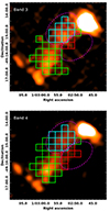 |
Fig. B.1. The two panels show the band 3 (top) and band 4 (bottom) images used in the spectral and point-to-point analysis. The two ellipses in magenta (dashed line) mark the two tails in X-rays. The regions of the grid within the two tails are color coded (cyan in the northern tail and red in the southern tail) in the point-to-point analysis. The rest of the regions are shown in green. |
All Tables
All Figures
|
Fig. 1. uGMRT band 3 image. The contours are overlaid on the point-source-subtracted Chandra X-ray image in color. The contour levels are −0.1, 0.1, 0.2, 0.4, etc. mJy beam−1. The positive radio contours are shown by the solid line (cyan), and the negative contours are shown by the dashed line (yellow). The synthesized beam size of the band 3 image is 14.5″ × 5.9″ and the position angle is 3.5°. The dashed blue segments indicate the northern and southern X-ray tails, respectively. |
| In the text | |
|
Fig. 2. uGMRT band 3 image in color and in contours. The contour levels are −0.1, 0.1, 0.2, 0.4, etc. mJy beam−1. The solid blue lines show the positive contours, and the negative contour is shown as the dashed gray line. The beam size is 14.5″ × 5.9″ and the position angle is 3.5°. The diffuse sources are labeled. The arrow indicates the new feature of the E relic that extends farther outward. The dashed segments mark the two X-ray tails. |
| In the text | |
|
Fig. 3. Left: uGMRT band 4 image in color and in contours. The beam is 9.6″ × 3.8″ and the position angle is 7.5°. Right: uGMRT band 5 image in color and in contours (blue shows positive and gray shows negative contours). The beam is 6.1″ × 2.4″ and the position angle is −0.81°. The contour levels in both panels are −0.04, 0.04, 0.08, 0.16, etc. mJy beam−1. The MeerKAT 1.28 GHz image (Knowles et al. 2022) with a resolution of 7.2″ × 6.6″ and a position angle of 44.6° is overlaid in red contours at levels of 15, 30, 60, etc. μJy beam−1. The rms in the MeerKAT image is 5 μJy beam−1. |
| In the text | |
|
Fig. 4. uGMRT band-4 image in color. The discrete sources are marked as circles and are labeled. The diamonds show the positions of the spectroscopically identified cluster members by Sifón et al. (2013). The source labels from L14 are shown, and two new labels C12 and C13 are added. The prefix U refers to sources that are unrelated to the cluster, and sources with the prefix C are cluster members. |
| In the text | |
|
Fig. 5. Integrated spectra of the diffuse sources in El Gordo. The open symbols show the points from L14. The solid lines show the power-law fits. The spectral indices are reported in Table 3. The dashed lines join the points for the respective diffuse components that were not included in the fits. |
| In the text | |
|
Fig. 6. Left: Spectral index map between 366 MHz and 672 MHz for the radio halo in El-Gordo at 15″ × 15″ resolution in color scale. The contours from the 672 MHz image at 0.1, 0.2, 0.4, 0.8, and 1.6 mJy beam−1 are overlaid. Right: Spectral index error map. High errors at the edges are expected due to the low S/N at the outskirts. The numbered regions used for analysis are shown in the map. The beam is shown in the top left corner in both panels. |
| In the text | |
|
Fig. 7. Spectral indices with error bars obtained from the spectral index map plotted as a function of the numbered regions shown in the right panel of Fig. 6. |
| In the text | |
|
Fig. 8. Left: Radio surface brightness (IR) vs. X-ray surface brightness (IX) for band 3. The points in these plots are from the grid shown in Figure B.1. The cyan points are from the northern X-ray tail, the red points are from the southern X-ray tail, and the remaining points are from the rest of the halo. The fit to the points is shown as a solid black line, and the 95% confidence region is shown in the shaded part. The dashed red line shows the 1σ level of the radio images. The light blue arrows indicate the upper limits above 2σrms points. Right:IR vs. IX scaling plot for band 4 in the same color-code as in the left panel. |
| In the text | |
|
Fig. 9. Spectral index (α)-X-ray surface brightness point-to-point comparison (filled blue circles). The error bars are statistical measurement errors. The best fit is shown with the solid black line, and the confidence interval is shown as the shaded region. |
| In the text | |
|
Fig. 10. Top left: X-ray temperature map in color. The dashed blue lines indicate the two X-ray tails that were shown in Fig. 1. Top right: Color map of the percentage error on the temperature (kT). The errors are dominated by the uncertainty on the temperature determination, which is ∼5% in the core region and ∼10% in the rest of the cluster. For the larger bins in the map, the temperature is not constrained. Bottom left: Pseudo-pressure map in logarithmic units in color. Bottom right: Entropy (K) map in color. The 672 MHz contours (cyan) from Figure 3 are overlaid in all the panels. |
| In the text | |
|
Fig. 11. Left: Fluctuation power spectrum in the central 1 Mpc of El Gordo, where the bullet is masked, as a function of wave number k. The red curve shows the 2D fluctuations in the power spectrum subtracted from the Poisson noise (blue curve). The green curve shows the corresponding deprojected 3D power spectrum. Right: Amplitude of 3D fluctuations |
| In the text | |
|
Fig. 12. 1.4 GHz radio power vs. mass (M500) plotted for El Gordo (this work and L14) with other samples of radio halos from the literature. The Di Gennaro et al. (2021a) sample consists of halos at redshifts > 0.6, the Knowles et al. (2021) contains radio halos in the redshift range of 0.22 < z < 0.65 and the local redshift (z ∼ 0.2) sample from Cassano et al. (2013). The recent discovery of the radio halo in ACT-CL J0329.2-2330 (z = 1.23) is also shown (Sikhosana et al. 2024). The large samples from the LOFAR survey by Botteon et al. (2022) (0.016 < z < 0.9), and from ASKAP by Duchesne et al. (2024) (0.01 < z < 0.5) have been added to provide a more comprehensive picture. |
| In the text | |
|
Fig. A.1. The uGMRT band 3 image with a resolution of 16″×16″ is shown in color with the regions used to measure the flux densities of the diffuse sources overlaid in dashed lines. |
| In the text | |
|
Fig. B.1. The two panels show the band 3 (top) and band 4 (bottom) images used in the spectral and point-to-point analysis. The two ellipses in magenta (dashed line) mark the two tails in X-rays. The regions of the grid within the two tails are color coded (cyan in the northern tail and red in the southern tail) in the point-to-point analysis. The rest of the regions are shown in green. |
| In the text | |
Current usage metrics show cumulative count of Article Views (full-text article views including HTML views, PDF and ePub downloads, according to the available data) and Abstracts Views on Vision4Press platform.
Data correspond to usage on the plateform after 2015. The current usage metrics is available 48-96 hours after online publication and is updated daily on week days.
Initial download of the metrics may take a while.