| Issue |
A&A
Volume 698, June 2025
|
|
|---|---|---|
| Article Number | A113 | |
| Number of page(s) | 15 | |
| Section | Planets, planetary systems, and small bodies | |
| DOI | https://doi.org/10.1051/0004-6361/202452302 | |
| Published online | 05 June 2025 | |
MIRI-JWST mid-infrared direct imaging of the debris disk of HD 106906
Structure and mass of the disk
1
LIRA, Observatoire de Paris, Université PSL, Sorbonne Université, Sorbonne Paris Cité, CY Cergy Paris Université, CNRS,
5 place Jules Janssen,
92195
Meudon,
France
2
Space Telescope Science Institute,
3700 San Martin Drive,
Baltimore,
MD
21218,
USA
3
Department of Physics & Astronomy, Johns Hopkins University,
3400 N. Charles Street,
Baltimore,
MD
21218,
USA
4
Université Paris-Saclay, Université Paris Cité, CEA, CNRS, AIM,
91191
Gif-sur-Yvette,
France
5
Department of Astrophysics/IMAPP, Radboud University,
PO Box 9010,
6500
GL
Nijmegen,
The Netherlands
6
HFML – FELIX. Radboud University
PO box 9010,
6500
GL
Nijmegen,
The Netherlands
7
SRON Netherlands Institute for Space Research,
Niels Bohrweg 4,
2333
CA
Leiden,
The Netherlands
8
Department of Astrophysics, University of Vienna,
Türkenschanzstrasse 17,
1180
Vienna,
Austria
9
Max-Planck-Institut für Astronomie (MPIA),
Königstuhl 17,
69117
Heidelberg,
Germany
10
ETH Zürich, Institute for Particle Physics and Astrophysics,
Wolfgang-Pauli-Strasse 27,
8093
Zürich,
Switzerland
11
Institute of Astronomy, KU Leuven,
Celestijnenlaan 200D,
3001
Leuven,
Belgium
12
STAR Institute, Université de Liège,
Allée du Six Août 19c,
4000
Liège,
Belgium
13
Centro de Astrobiología (CAB), CSIC-INTA, ESAC Campus, Camino Bajo del Castillo s/n,
28692
Villanueva de la Cañada, Madrid,
Spain
14
School of Physics & Astronomy, Space Park Leicester, University of Leicester,
92 Corporation Road,
Leicester,
LE4 5SP,
UK
15
UK Astronomy Technology Centre, Royal Observatory,
Blackford Hill,
Edinburgh
EH9 3HJ,
UK
16
Université Paris-Saclay, CEA, IRFU,
91191,
Gif-sur-Yvette,
France
17
Department of Astrophysics, American Museum of Natural History,
New York,
NY
10024,
USA
18
Jet Propulsion Laboratory, California Institute of Technology,
4800 Oak Grove Dr.,
Pasadena,
CA
91109,
USA
19
Aix Marseille Univ, CNRS, CNES, LAM,
Marseille,
France
20
Department of Astronomy, Oskar Klein Centre, Stockholm University,
106 91
Stockholm,
Sweden
21
School of Cosmic Physics, Dublin Institute for Advanced Studies,
31 Fitzwilliam Place,
Dublin,
D02 XF86,
Ireland
★ Corresponding author: This email address is being protected from spambots. You need JavaScript enabled to view it.
Received:
19
September
2024
Accepted:
30
March
2025
Abstract
Context. We report MIRI-JWST coronagraphic observations at 11.3 and 15.5 μm of the debris disk around the young star HD 106906. The wavelength range is sensitive to the thermal emission of the dust heated by the central star.
Aims. The observations were made to characterize the structure of the disk through the thermal emission, to search for clues to the presence of a central void of dust particles, and to derive the mass of the dust and the temperature distribution. Another goal was also to constrain the size distribution of the grains.
Methods. The data were reduced and calibrated using the JWST pipeline. The analysis was based on a forward-modeling of the images using a multiparameter radiative transfer model coupled to an optical code for coronagraphy processing.
Results. The disk is clearly detected at both wavelengths. The slight asymmetry is geometrically consistent with the asymmetry observed in the near-IR, but it is inconsistent the brightness distribution. The observed structure is well reproduced with a model of a disk (or belt) with a critical radius 70 au, a mildly inward-increasing density (index 2) and a steeper decrease outward (index −6). This indication of a filled disk inside the critical radius is inconsistent with sculpting from an inner massive planet. The size distribution of the grains that cause the mid-IR emission is well constrained by the flux ratio at the two wavelengths : 0.45–10 and 0.65–10 μm for silicate and graphite grains, respectively. The minimum size is consistent with predictions of blowout through radiative pressure.
Conclusions. We derive a mass of the dust that causes the mid-IR emission of 3.3–5.0 10−3 M⊕. When the larger grains (up to 1 cm) that cause the millimeter emission are included, we extrapolate this mass to 0.10–0.16 M⊕. We point out to that this is fully consistent with ALMA observations of the disk in terms of dust mass and of its millimeter flux. We estimate the average dust temperature in the planetesimal belt to be 74 K, but the temperature range within the whole disk is rather wide: from 40 to 130 K.
Key words: circumstellar matter / planetary systems / infrared: planetary systems
Based on observations collected with JWST through observing proposals 1277, and 1241.
© The Authors 2025
 Open Access article, published by EDP Sciences, under the terms of the Creative Commons Attribution License (https://creativecommons.org/licenses/by/4.0), which permits unrestricted use, distribution, and reproduction in any medium, provided the original work is properly cited.
This article is published in open access under the Subscribe to Open model. This email address is being protected from spambots. You need JavaScript enabled to view it. to support open access publication.
1 Introduction
Debris disks are dusty disks that are most often found around young main-sequence and pre-main-sequence stars. They can help us to characterize one important phase in the initial evolution of exoplanetary systems. They are produced through collisional cascades, in which planetesimals break into millimeter to submicron-sized dust grains (Wyatt 2008; Matthews et al. 2014; Hughes et al. 2018).
Most of debris disks are detected through their far-IR excess, such as the archetypical excess around β Pic that was discovered by the IRAS satellite1 and then observed in the visible (Aumann 1984; Smith & Terrile 1984). Since the advent of near-IR instruments with a high angular resolution that use adaptive optics and are installed on large telescopes, the direct detection of the light that is scattered by grains of the disk became another powerful way to study debris disks (Hughes et al. 2018). The additional benefit of these instruments is that they provide structural information. Efficient scattering implies grains of a relatively small size. However, under the action of radiation pressure and/or stellar winds, dust grains that are smaller than a critical size must be blown out from the system on a timescale that is short enough to require that the collisional cascade continually produces small dust grains to replenish the disk (Augereau & Beust 2006; Strubbe & Chiang 2006). This requires that the relative velocity of the planetesimals is sufficient to cause fragmentation upon impact. The question of the grain size distribution is then important and is directly related to the mechanisms of grain replenishment, blowout, and fragmentation that occur in the early phase of planet formation. Mid-IR resolved imaging is also an efficient means for studying the grain population in debris disks. By probing the thermal emission of the dust, it can constrain the size distribution of medium-size grains, their distribution in the disk, and their temperature, and it provides a more reliable estimate of the total grain mass.
In the following, we present observations of the debris disk around the binary system HD 106906 that were obtained using the Mid-Infrared Imager (MIRI) aboard the James Webb Space Telescope (JWST) in its coronagraphic mode. The disk is indeed detected in the two filters F1140C (11.3 μm) and F1550C (15.5 μm), and we derived several pieces of information on its structure and its luminosity. Because of its small angular size, the disk is partly attenuated by the effect of the coronagraph. To proceed, we present an attempt to reproduce the observed fluxes and the spatial distribution of light using a radiative transfer model. The code takes scattering and thermal emission as well as a parameterized structure of the disk into account. From the comparison of the best-fit model to the observations, we derived several important quantities: the grain size distribution, the mass of the disk, the temperature map, and the structure. Section 2 summarizes what is known about the HD 106906 system. Section 3 describes details of the observations. Section 4 provides elements of the data reduction and calibration. In Sect. 5 we show the resulting images at the two observation wavelengths. Section 6 describes the components of the radiative transfer code we used. In Sect. 7 we analyze the output of the code for a grid of 96 different sets of parameters and compare them to observations to determine the best-fit model of the disk and the grain population. In Sect. 8 we discuss the results for the structure of the disk, the mass, and the temperature of the disk. We also discuss this in terms of consistency with other observations and theoretical works.
Log of observations.
2 HD 106906
HD 106906 (HIP 59960) is a pre-main-sequence F5V-type binary stellar system (Absil et al. 2021; De Rosa & Kalas 2019; separation: 0.14 au, PA: 95.2°) featuring a debris disk and an 11 MJup planet companion (Bailey et al. 2014) at an unusually large projected separation of ≈800 au. Lagrange et al. (2016) estimated a physical distance between 2000 and 3000 au based on the assumption that the planet orbit is coplanar with the disk. The system is a member of the lower Centaurus Crux (LCC) association, which has a mean age of 17 ± 5 Myr, which agrees with an isochronal age and mass of 13 ± 2 Myr and 1.35 M⊙ for each component of the binary star (Pecaut et al. 2012; Rodet et al. 2017). The debris disk was first detected by the Spitzer satellite based on its infrared excess (Chen et al. 2005) and was later observed at near-IR wavelength by Kalas et al. (2015) with the Gemini Planet Imager (GPI), by Lagrange et al. (2016) (quoted as L16 in the following) using the instrument Spectro Polarimetric High contrast Exoplanet REsearch (SPHERE) on the Very Large Telescope (VLT), and by Crotts et al. (2021) in polarimetry in the J, H, and Ks bands. The disk is elongated in the SE-NW direction and is seen nearly edge-on. It extends beyond 100 au, and its brightness distribution peaks at about 65–75 au. Using a geometrical model to account for scattering, L16 derived an inclination of 85.3 ± 0.1° and a disk position angle (PA) of 104.4 ± 0.3°. More recently, Kral et al. (2020) and Fehr et al. (2022) detected and resolved the thermal emission of the disk at the millimeter wavelength using the Atacama Large Millimeter/submillimeter Array (ALMA), but did not detect CO.
3 Observations
HD 106906 is included in MIRIco, which is an EU and US coordinated observing effort that makes use of MIRI (Wright et al. 2023) in its coronagraphic mode throughout programs 1277 and 1241. The target was observed in one run on May 16, 2023, under Guaranteed Time Observations (GTO) program 1277, using the MIRI Four Quadrant Phase Mask (Rouan et al. 2000) coronagraphs (4QPM) with filters F1140C and F1550C.
The goal of the program is to characterize the planet and the disk. This paper is essentially devoted to the study of the disk, and a forthcoming paper will focus on the planet photometry. The observation log is provided in Table 1. For each coronagraphic filter, we observed the target and its associated background back to back (in two dithers). The background images were used to remove the glowstick effect, as explained by Boccaletti et al. (2022), and they were obtained near the target (typically, a few dozen arcseconds away). Unlike for the observations of HR 8799 and HD 95086 (Boccaletti et al. 2024; Mâlin et al. 2024), we did not observe a dedicated reference star. The reference star we used here to subtract the residues is HD 218261. This star was also used by Boccaletti et al. (2024) for HR 8799 and was observed in November 2022, so there is a gap of almost 6 months. The stability of JWST is good enough for the subtraction to be fully efficient, however. The reference has a comparable magnitude to HD 106906 in the MIRI coronagraphic filters. Taking into account the stellar residuals and the background noise from the diffraction model of Boccaletti et al. (2015), we determined the exposure times to achieve signal-to-noise ratios (S/N) higher than ≈10 on the planet. The total exposure times on target were 360 s and 1800 s for the F1140C and F1550C filter, respectively.
4 Data reduction and calibration
We retrieved the processed data from the Mikulski Archive for Space Telescopes (MAST2), and we also reprocessed the raw data on our side with v12 of the JWST pipeline3 (Bushouse et al. 2025) for comparison. The main steps of the process were the same as in Boccaletti et al. (2024); Mâlin et al. (2024). In brief, stage 1 of the JWST pipeline applies ramps-to-slopes processing and delivers count-rate images corrected for various detector artifacts (linearity, saturation, outliers, etc.). Stage 2 is reduced to only applying the background subtraction without any flat correction to avoid increasing noise and the glowstick effect. We verified that the impact on the photometry is lower than 2%, which is much smaller than the other sources of noise (Boccaletti et al. 2024). In the end, we collapsed all integrations (Nint) into a single frame to obtain a number of frames that was the number of dither positions (Ndither). A mean combination of the background dithers was subtracted from each target observation, and the remaining bad pixels were rejected with a σ clipping.
Each coronagraphic image was registered at the 4QPM centers. This was determined during commissioning (using a cross-correlation with a large database of simulated data).
Raw coronagraphic images are essentially dominated by the diffraction pattern proper to the hexagonal pupil of the JWST. The optimized Lyot stop cannot completely suppress this (Boccaletti et al. 2022). We performed reference differential imaging (RDI) with a single reference star and considered several approaches, including PCA and linear combination as in Boccaletti et al. (2024) and Mâlin et al. (2024). As a result, we selected the simplest RDI method, which uses a single image of the reference star obtained at one out of the nine positions of the small grid dither. This position and the intensity scaling were chosen to minimize the diffraction residuals while maximizing the disk intensity.
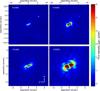 |
Fig. 1 Top: MIRI F1140C (left) and F1550C (right) full-field coronagraphic images after data reduction (see text) and reference subtraction. The planet HD 106906 b can be seen at 7.3 arcsec NW. Bottom: same after zooming and binning by a factor 2. The orientation is standard (north is up, and east is to the left). The field of view is 22 × 22 arcsec2 at the top and 11 × 11 arcsec2 at the bottom. |
5 Resulting images
Figure 1 displays the reduced images resulting from the process described above at the two wavelengths 11.4 and 15.5 μm and the same after zooming on the central part and binning by a factor of two. The disk clearly appears as two elongated patches in the processed images that bracket a void that is caused by the coronagraph extinction of the central part of the disk. The direction joining the two centers of gravity of the patches has a PA of 112°, which is significantly larger than the PA measured in nearIR (104.4° for L16, 103.7° for Kalas et al. 2015, 103° for Fehr et al. 2022). We note that a first reason for a difference between near-IR and mid-IR orientation of the disk is that it appears rather as an arc in the near-IR because only the scattering edge is seen. Second, we point out that this difference is not expected to be related to the difference between mechanisms of emission that are at play in each wavelength domain (scattering versus thermal emission). This appears to be obvious when the final images produced by the model are analyzed. (see Section 6). They feature the same pattern as in the observed image, where the line joining the two lobes has the same orientation, while the model produces an initial image (before processing by the coronagraph) that is fully symmetric with respect to the imposed direction of PA = 104.4°. We argue that this is the result of some diffraction effects induced by the four-quadrant coronagraph mask, and we note that the direction with respect to the north of the frontier between the quadrants is 4.83° and that this must have some effect on the polar angle of the observed structures in the resulting image.
In addition to the patches, two fainter hook-like structures are observed. They start from one side of each patch and describe a centro-symmetric pattern analogous to spiral arms. We discuss this peculiar feature further below and show that it provides a good indicator for constraining the radial structure of the disk. We note that the two patches are not rigorously symmetric, and we discuss this point in Sect. 8.
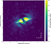 |
Fig. 2 MIRI 11.4 μm coronagraphic image. The contours of the SPHERE H1-H2 image of Lagrange et al. (2016) are superimposed. |
6 The disk model
The appearance of the disk in the mid-IR is substantially different from what is observed in the near-IR wavelength in scattered light, as shown in Fig. 2, where the contour of the SPHERE image at H (Lagrange et al. 2016) is superimposed on the MIRI 11.4 μm coronagraphic image. The differences arise from three factors: the lower angular resolution, the attenuation of the 4QPM in its transition directions, and the thermal emission compactness, which concentrated the observed light in the parts closest to the star. It is then much more difficult than at near-IR to interpret MIRI images straightforwardly in terms of structure, extension, and inclination of the disk.
In order to constrain the structure of the disk and to account for the measured fluxes in the two filters, we proceeded by forward-modeling a physical model of the disk through the diffraction model of the MIRI coronagraph. We started with the code DDiT described by Olofsson et al. (2020) and modified it to include several features that were not present in the open-source Python version that is available on GitHub4. Essentially, all the parts of the code concerning the propagation of light from the star to the disk and from the disk to the observer are preserved, and this also holds for the dust density calculation using the parameterized distribution proposed by Augereau et al. (1999). For our purpose, we added
the use of wavelength-dependent optical properties of grains, that is, essentially, the tables from Laor & Draine (1993) for Qabs, Qsca, and gsca;
the distribution of the grain sizes. We only used the classical a−3.5 power law. This law is expected from an equilibrium collisional cascade (Dohnanyi 1968) and was also proposed for the interstellar medium by Mathis et al. (1977) (the so-called MRN law; the code can manage any power law);
a true computation of the radiative equilibrium temperature of grains and of the corresponding thermal emission. For that purpose, we solved for each grain with a radius a the radiative equilibrium equation
![Mathematical equation: $\[\int Q_{a b s}^{a}(\lambda) ~J~(\lambda) ~\mathrm{d} \lambda= \int Q_{a b s}^{a}~(\lambda) ~4 \pi ~B~(\lambda) ~\mathrm{d} \lambda\]$](/articles/aa/full_html/2025/06/aa52302-24/aa52302-24-eq1.png) , where J(λ) is the mean radiation intensity at wavelength λ, and B(λ) is the Planck function;
, where J(λ) is the mean radiation intensity at wavelength λ, and B(λ) is the Planck function;the radius and temperature of the star in order to produce a realistic stellar spectrum;
an actual value of the returned fluxes (in μJy) for scattered light and thermal radiation instead of proportional quantities.
The code (which we refer to as DDiT+ in the following) produces maps of the flux as well as maps of the averaged temperature on the line of sight.
The parameters that were used or adjusted in the simulations were the size of the critical radius of the disk, Rc; the distance in parsec; the wavelength; the minimum and maximum grain radii, amin and amax. As regards the nature of grains (silicate or graphite), we favored silicate grains for two reasons: (i) as noted by Hughes et al. (2018), Spitzer spectroscopy of a large sample of debris disks revealed that their dust composition is dominated by standard silicates, and (ii) the Spitzer spectrum of HD 106906 (https://cassis.sirtf.com/atlas/) reveals two features in emission at 23.7 and 34.0 μm that likely are characteristic of forsterite crystalline silicate (Vandenbussche et al. 2004) (see Fig. D.1, where the features are tentatively identified on the spectrum). Note that we also considered graphite grains in order to assess the sensitivity of the model results to the grain nature. We also adjusted the αin and αout exponents of the surface density as described by Augereau et al. (1999); the inclination; the position angle; the mass of the disk; the radius and effective temperature of the star (which we considered to be a unique star).
The eccentricity was set to zero. We mainly varied the parameter αin in the disk structure, which sets the contribution of the innermost part of the disk. Roughly speaking, when αin = 10, the slope of the density variation is extremely steep, and the disk is essentially considered to be a ring at the critical radius, while with αin = 1, the density increases continuously from the center to the critical radius. This results in a filled disk. When scattered light at near-IR was modeled, the slope of the outer radius was generally considered to be rather steep (Kalas et al. 2015; Lagrange et al. 2016). We therefore varied αout between −4 and −10 in the simulations. Only Crotts et al. (2021) proposed a fainter slope of −2.26, which was based on radiative transfer modeling. The value −4 was generally considered when the external part was dominated by blowout.
We divided the range of grain sizes into bins (typically, 10–20), and we computed for each bin the fraction of the total mass to which this bin corresponded. We ran the model using the proper grain optical properties. We then computed the sum of all intensities weighted by the corresponding fraction of mass to obtain the final intensity map. This was done for the scattered light and for the thermal emission by the disk.
The question of the dust size distribution law in HD 106906 was discussed before. For instance, Crotts et al. (2021) considered a power law with an index q = −3.19. As noted by Farhat et al. (2023), this distribution differs only slightly from that of a collisional cascade, which is characterized by q ≈ −3.5 (Dohnanyi 1968). We considered medium-size grains, which are less involved in near-IR scattering, and we therefore chose to retain the collisional cascade index.
The mass of the disk plays no role in the calculation, except for the value of the flux, which is directly proportional to the mass. For this reason, all our computations were made with a mass of 1 M⊕. By comparing the resulting total flux to the measured flux, we derived the mass of the disk for the considered grain population. This is a minimum mass because larger grains are probably present, but do not contribute to the flux at mid-IR wavelengths, as we discuss below.
After we produced the final intensity map, we used it as input to a code that simulated the effect of the optical system of the JWST + MIRI coronagraphic channel as realistically as possible. It took the actual shape and aberrations of the primary mirror, the shadow by the secondary struts, the effect of the 4QPM, and the optimized Lyot stop into account. Because the disk is somewhat fainter than the star, this simulation of synthetic disk images did not include any potential broadening through electronic effects, which is referred to as the brighter-fatter effect (Argyriou et al. 2023). This effect appears to be negligible. The output image was then compared to the observed image, and we evaluated the quality of the fit by computing the reduced ![Mathematical equation: $\[\chi_{\nu}^{2}\]$](/articles/aa/full_html/2025/06/aa52302-24/aa52302-24-eq2.png) between the data and the model. The complete modeling (radiative transfer plus optical system) allowed us to estimate the attenuation by the coronagraph channel. The attenuation depends on the object and is radically different for a point source (as estimated in Boccaletti et al. 2024) and a central extended object. For instance, we measured a total attenuation for the range of models that varied from ~1.8 to 3.4 at F1140C.
between the data and the model. The complete modeling (radiative transfer plus optical system) allowed us to estimate the attenuation by the coronagraph channel. The attenuation depends on the object and is radically different for a point source (as estimated in Boccaletti et al. 2024) and a central extended object. For instance, we measured a total attenuation for the range of models that varied from ~1.8 to 3.4 at F1140C.
Several parameters were fixed once for all, such as the distance (103 pc), because it is strongly constrained by Gaia-DR3 (Gaia Collaboration 2023); the position angle and the inclination because they are well determined by near-IR studies (Kalas et al. 2015; Lagrange et al. 2016; Crotts et al. 2021); the radius; and the effective temperature of the star, whose spectral type is well determined. We fixed the effective temperature at 6900 K and the radius at 1.7 R⊙, so that the total bolometric luminosity of 5.9 L⊙ was similar to the theoretical luminosity of two identical F5V stars (De Rosa & Kalas 2019). The analyses of the structure of the disk was based on models using silicate grains only.
To discuss the disk mass, we also considered graphite grains (see Sect. 8.2).
List of parameter values we used to build the grid of models.
7 Comparing model and observations
7.1 Building a grid of models
Using rather conservative parameters taken from near-IR studies and a broad grain size range (0.1–10 μm), we first compared the scattered and thermal intensities to conclude that the former was always several orders of magnitude lower than the latter at the wavelength of interest for MIRI coronagraphy. Therefore, we only consider the thermal component in the following. Several parameters can be adjusted, and we therefore adopted the following procedure: to determine the best morphological fit between the simulated coronagraphic images and the observed images, we first considered a grid of 96 (2 × 3 × 4 × 4) models that each corresponded to a combination of four parameters: λ, Rc, αin, and αout. We then computed the disk image as an input to the coronagraphic numerical process for each (see Fig. C.1) and compared the output to the actual observed image with a χ2 metrics. When a good agreement was found, we varied different grain size ranges in a second step, until amin and amax matched the observed ratio F15.5/F11.4 well, that is, until they reached a value in the middle of the uncertainty range, as shown in Fig. 7. Table 2 gives the complete set of values we used for each of these parameters to build the grid of models.
A peculiar feature in the observed images played an important role in refining the fit: the hook-like structures previously mentioned that depart from each lobe. They correspond to some diffraction effects, and only certain sets of parameters produced their shape and location correctly. We were able to reproduce them only for a rather narrow range of Rc and of αin. As an illustration, we display in Fig. 3 the observed images, different results (among the best) of the simulation for different sets of λ, Rc, αin, and αout, and the residue maps. The simulation clearly provide fairly similar results to the observed images.
In Table 3 we list the selected combinations of parameters that produced the lowest value of ![Mathematical equation: $\[\chi_{\nu}^{2}\]$](/articles/aa/full_html/2025/06/aa52302-24/aa52302-24-eq3.png) (v standing for the degree of freedom) for λ = 15.5 μm and 11.4 μm, sorted from lowest to highest
(v standing for the degree of freedom) for λ = 15.5 μm and 11.4 μm, sorted from lowest to highest ![Mathematical equation: $\[\chi_{\nu}^{2}\]$](/articles/aa/full_html/2025/06/aa52302-24/aa52302-24-eq4.png) . The
. The ![Mathematical equation: $\[\chi_{\nu}^{2}\]$](/articles/aa/full_html/2025/06/aa52302-24/aa52302-24-eq5.png) is calculated in an elliptical aperture encompassing the disk, of 1.8″ the major axis, and containing 593 pixels, which cannot be considered independent since the angular resolution is 3.2 and 4.4 pixels for F1140C and F1550C, respectively. Therefore, we took into account the surface of the PSF in the calculation of the degree of freedom, as well as the number of parameters in the geometric model (Rc, αin, and αout). The sets that give the lowest
is calculated in an elliptical aperture encompassing the disk, of 1.8″ the major axis, and containing 593 pixels, which cannot be considered independent since the angular resolution is 3.2 and 4.4 pixels for F1140C and F1550C, respectively. Therefore, we took into account the surface of the PSF in the calculation of the degree of freedom, as well as the number of parameters in the geometric model (Rc, αin, and αout). The sets that give the lowest ![Mathematical equation: $\[\chi_{\nu}^{2}\]$](/articles/aa/full_html/2025/06/aa52302-24/aa52302-24-eq6.png) are not the same for the two wavelengths, but the variation in
are not the same for the two wavelengths, but the variation in ![Mathematical equation: $\[\chi_{\nu}^{2}\]$](/articles/aa/full_html/2025/06/aa52302-24/aa52302-24-eq7.png) is also not very large: ±11% for the 12 listed sets at 15.5 μm, and ±3% for the 8 sets at 11.4 μm. We decided to only retain the set of parameters that was common to both wavelengths. For this set,
is also not very large: ±11% for the 12 listed sets at 15.5 μm, and ±3% for the 8 sets at 11.4 μm. We decided to only retain the set of parameters that was common to both wavelengths. For this set, ![Mathematical equation: $\[\chi_{\nu}^{2}\]$](/articles/aa/full_html/2025/06/aa52302-24/aa52302-24-eq8.png) is only 22 and 3.5% higher than the lowest value at 15.5 μm and 11.4 μm, respectively. This set of parameters, indicated in bold in Table 2, features Rc = 70 au, αin = 2, and αout = −6. Figure 4 shows the processed images corresponding to this set of parameters. We confirmed this result with a criterion that multiplied the
is only 22 and 3.5% higher than the lowest value at 15.5 μm and 11.4 μm, respectively. This set of parameters, indicated in bold in Table 2, features Rc = 70 au, αin = 2, and αout = −6. Figure 4 shows the processed images corresponding to this set of parameters. We confirmed this result with a criterion that multiplied the ![Mathematical equation: $\[\chi_{\nu}^{2}\]$](/articles/aa/full_html/2025/06/aa52302-24/aa52302-24-eq9.png) for each filter. The minimum value was obtained for this very same model: Rc = 70 au, αin = 2, and αout = −6. We consider this set as the best fit below.
for each filter. The minimum value was obtained for this very same model: Rc = 70 au, αin = 2, and αout = −6. We consider this set as the best fit below.
7.2 The structural parameters
We determined how these quantities compared to previous estimates. Lagrange et al. (2016) and Kalas et al. (2015) used Rc = 65 au and a distance of 92 pc at a time when this distance was not firmly established. This translates into 74 au at 103 pc, the Gaia distance, which is the most reliable estimate we can use today. We note that our best value of Rc is similar to the value deduced from a radiative transfer modeling of the GPI data by Crotts et al. (2021). Because our best fit is for αout = −6, indicating an external radius that is not so steeply defined, we considered that the near-IR and mid-IR determinations of the critical radius agree well, and we conclude that the grains that cause the thermal emission are located at the same distance as those that cause the near-IR scattering. With αin = 2, we cannot consider the dust grain population to which we are sensitive at mid-IR as concentrated in a narrow ring coincident with the birth ring of planetesimals, but it instead extends well toward the center. This agrees with Bailey et al. (2014), who reported a disk extending from 20 to 120 au based on the Ks and L’ fluxes, while Fehr et al. (2022) deduced a radially broad axisymmetric disk with radii between 50 and 100 au based on millimeter emission. This result does not contradict the fact that in scattered near-IR light, the appearance of the disk suggests a void. The small grains (a ~ 1 μm) scatter light at near-IR proportionally to their mass fraction, but emit far more strongly in the mid-IR than their mass fraction because they are hottest and the flux in the mid-IR depends exponentially on the temperature (Wien part of the Planck’s function), as illustrated in Fig. 5. A relatively low density of small grains may therefore result in a very significant mid-IR flux. This behavior, which is specific to the mid IR range, was well described theoretically in Thebault & Kral (2019).
The total flux for the disk provided by DDiT+ at each wavelength was evaluated in two ways, using either the real data and taking the attenuation of the coronagraph derived from the total flux ratio of the noncoronagraphic to coronagraphic synthetic images into account (method 1), or in the noncoronagraphic synthetic image given the intensity scaling to match the coronagraphic data and its corresponding model in the χ2 process (method 2). For the best model (a70pi2po6), we measured a coronagraphic attenuation of 3.0 and 2.5 for F1140C and F1550C, respectively. We calculated the mean and the standard deviation of the flux obtained by the model in Table 3 and for the two flux extraction methods. The values we retained in the following are those corresponding to an average of the best models: 1223 ± 20 μJy and 7230 ±470 μ Jy at F1140C and F1550C, respectively.
7.3 Flux ratio and grain size
After we established the structure of the disk, we reproduced the observed flux ratios Rf = F15.5/F11.4 = 5.91 ± 0.50 by adjusting the range of grain sizes and the nature of grains. The bins of the size follow a geometrical progression of reason 1.38, starting from amin.
Because the mass fraction associated with each bin of size increases from amin to amax while the corresponding fluxes decrease at both wavelengths (Fig. 5), it is not intuitive to predict the range that fits the observed ratio best. For instance, we plot in Fig. 6 the ratio Rf versus the grain size for a population of grains with a unique size. From the analysis of this figure, we could be tempted to conclude that the maximum size should not be much larger than 1 μm for silicate and 2.5 μm for graphite, because larger grains, when considered alone, produce much higher values of the ratio Rf. This is not the case, however, and we show in Fig. 7 various attempts to reproduce the ratio with different choices of amin and amax. This figure indicates that the range should include grains of size ~1–2 μm, but a good fit of the observed ratio is reached for silicate grains in the range 0.45–10 μm and for graphite grains in the range 0.65–10 μm, as shown in Fig. 7 where these ranges are indicated by thicker segments. A rather wide range of sizes is needed to reproduce the flux ratio, as expected, because in the standard picture of a debris disk, a continuous collisional cascade starts at large (unseen) parent bodies and extends to micron-sized dust that is blown out by radiation pressure (e.g., Thébault & Augereau 2007). The minimum silicate grain size of 0.45 μm appears to be consistent with the value that is generally assumed based on the spectral analysis of the mid-infrared silicate feature (Mittal et al. 2015). Moreover, this value is close to the theoretical threshold in radius corresponding to blowout (see the discussion in Sect. 8.1). The polarizability curve may also indicate a submicron minimum grain size, such as in the case of AU Mic (Graham et al. 2007). In the following, we consider two sets of parameters that give a reasonable fit to the observations. Both have in common αin = 2, αout = −6, Rc = 70 au, for silicate grains, amin = 0.45 μm and amax = 10 μm, and for graphite grains, amin = 0.65 μm and amax = 10 μm. We base the remaining discussion on these two sets.
 |
Fig. 3 Comparison of simulated coronagraphic images and the observed image for a few cases for which the set of parameters αin, αout, and Rc led to a rather good solution, as indicated by the low residue level (second row of each set). The two upper rows correspond to the F1140C filter, and the two bottom rows show the F1550C filter. The label at the top of each image lists the values of the parameters in short. For example, a65pi1po4 stands for Rc = 65 au, αin = 1, and αout = −4. |
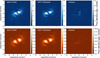 |
Fig. 4 Comparison of the observed coronagraphic images (left) and the best simulated images (center). The residuals of the difference are plotted at the right. |
 |
Fig. 5 Disk fluxes (in arbitrary units) at 15.5 μm (red) and 11.4 μm (green) emitted by each bin of grain size, as predicted by DDiT+. Only the case of silicate grains is shown here. |
Parameters for the set of best models at 15.50 and 11.40 μm.
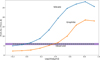 |
Fig. 6 Ratio Rf = F15.5/F11.4 vs. grain size for a single grain size, as given by the DDiT+ model. In blue, we show the case of silicate grains, and in orange, we show the case of graphite grains. The range of ratios deduced from observations is indicated by the shaded purple rectangle. |
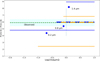 |
Fig. 7 Dependence of the ratio Rf = F15.5/F11.4 on the grain size distribution. The ratio Rf is deduced from the model after integration of the flux in the considered size range. Rf is plotted for a selection of different size ranges, all following a distribution in a−3.5. Each segment depicts a range that is plotted in blue for silicate grains and in orange for graphite grains. The dots correspond to single sizes of silicate grains. The two retained ranges are indicated by thicker dash-dot segments. The range of ratios deduced from observations is indicated by shaded cyan rectangle. |
8 Discussion
8.1 Structure of the disk
In order to reproduce the observed images, the parameter αin of the model can never be larger than 2, indicating an internal disk populated with dust, while near-IR observations by Kalas et al. (2015) and Lagrange et al. (2016) would rather argue for a marked void, possibly generated by an inner planetary systems within a distance of 50 au. Interestingly, a power-law index of αin = 2 like this is predicted in the case of a purely collisional evolution of a debris disk, as stated by Pearce et al. (2024), who proposed an analytic model to investigate the effect of a sculpting planet on the radial surface-density profile at the inner disk edge. This is often considered as a lack of an internal planet that would otherwise produce a gap or a steep inner edge, as predicted by several models (Ertel et al. 2012; Dong & Dawson 2016; Imaz Blanco et al. 2023), or observed in numerous cases (Esposito et al. 2020), for instance, in the emblematic system of PDS 70 (Müller et al. 2018; Keppler et al. 2018; Christiaens et al. 2024; Jang et al. 2024; Perotti et al. 2023), where the planets carving the cavity are indeed detected. To illustrate how MIRI images would be sensitive to differences in profiles resulting from a gap, we considered the case of a simulated gap with αin = 6, αout = −6. We plot in Fig. 8 the intensity profiles at 11 and 15 μm for this case and for our nominal case (αin = 2, αout = −6). This gap remains somewhat shallow, however, when we consider that the quantity σi defined by Pearce et al. (2024) to quantify the flatness of the inner edge is 0.32 (applying their equation (C1) to convert αin = 6 into σi), that is, it is still in the range that is incompatible with the planet-sculpting only case according to their Fig. 16. Again, we would tend to conclude that there is no massive planet inside the disk. Nevertheless, Pearce et al. (2024) listed no fewer than 11 reasons that could cause inner edges that are flatter than expected from sculpting planets. Finally, we recall that, as discussed above, MIRI does not sense the same range of grain sizes in the thermal IR as in near-IR, which is entirely dominated by scattering. The two grain populations likely follow a different spatial distribution. Therefore, the MIRI observations do not exclude the more or less significant presence of dust inside the disk, depending on the grain size.
Another point regarding the structure of the disk is, as already noted, the slight asymmetry between the two lobes. The ESE lobe extends slightly farther to the ESE, while the WNW lobe is slightly brighter and extends slightly more northward. This can be observed in particular in the 11.4 μm image of Fig. 1 and even more in the right column of Fig. 4, where the difference between the observed image and the image obtained with the model giving the best fit is displayed at each wavelength. The regions in which the symmetry is broken are enhanced. They appear to be similar at the two wavelengths. The relative increase in the brightness is about 20% ±3.5%. This asymmetry is to be compared to the one noted in the near-IR images (Kalas et al. 2015; Lagrange et al. 2016), which clearly appears in Fig. 2, where the near-IR contours describe a greater vertical width for the WNW lobe. Nguyen et al. (2021) described the eastern side of the disk as vertically thin and more extended than the western side of the disk, which is vertically thick. This description is consistent with what we observe in the mid-IR. In terms of brightness, however, we rather note an anticorrelation between the mid-IR and near-IR, the latter exhibiting a brighter SE extension. This might suggest that as in the Fomalhaut disk (Pan et al. 2016), the disk is eccentric and shows an anticorrelated apocenter brightnesses between the near-IR and mid-IR, but some care must be exercised because on one hand, the HD 106906 disk is seen quasi edge-on, an unfavorable situation to conclude on its eccentricity, and on the other hand, there is no universal rule on this apocenter anticorrelation, as stated by Lynch & Lovell (2022), who reported that at shorter wavelengths the classical pericenter glow effect remains true, whereas at longer wavelengths disks can either demonstrate apocenter glow or pericenter glow, depending on the observational resolution. Finally, models showed that at 15 μm, the effect might be undetectable (see Fig. 3 of Pan et al. 2016). The difference of the asymmetry between the near-IR and mid-IR can be attributed to the coexistence of several types of grains in the disk and/or a variable dust density, as proposed by Mazoyer et al. (2014) (see the discussion of the grain size below).
This asymmetry was proposed to be the result of gravitational perturbations by the planet, even though it is very distant (Nguyen et al. 2021; Nesvold et al. 2017). This would require either a high eccentricity for the planet (Nesvold et al. 2017 propose e = 0.7) or a high relative inclination between the disk and the planet orbit: for instance Nguyen et al. (2021) proposed 36 or 44°, but the error bars are quite large. On the other hand, the N-S asymmetry can tentatively be interpreted as the trace of a vertical warping that might result from a recent close encounter either with a star De Rosa & Kalas (2019) or with a free-floating planet, as proposed by Moore et al. (2023). The binary star at the center may also be at the origin of this asymmetry by introducing some gravitational perturbation in the disk.
The minimum grain size (0.45 μm for silicates) derived from the flux ratio in the two filters agrees with the theoretical estimates of Kirchschlager & Wolf (2013), who found a blowout size of 0.455 μm for nonporous grains (see their table 3). This is about twice smaller than the blowout size (0.85 μm) estimated by Crotts et al. (2021), however. This situation was also reported in other debris disks and was often associated with a blue color (Bhowmik et al. 2019; Debes et al. 2008; Augereau & Beust 2006), but it seems to contradict the findings of Crotts et al. (2021), who found a bimodal distribution that peaked at 0.91 μm (i.e., consistent with the blowout size) and 3.17 μm (consistent with a neutral color). However, the blowout size concept does not prevent smaller dust grains from being present in the system because they are continuously produced by collisional cascades in steady state (Thebault & Kral 2019), which can occur for debris disks with a high fractional luminosity (fd > 10−3). We also recall that near-IR polarimetric observations in scattered light presented by Crotts et al. (2021), and these mid-IR observations in the thermal regime, are sensitive to different grains sizes and properties and also to different regions of the disk. For instance, as demonstrated by the value we obtained for the inner slope of the surface density, MIRI sees a population of dust grains inside the birth ring of planetesimals because of their high temperature, and hence, a significant mid-IR emission. The values of αin and amin are likely linked and consistent, as discussed by Thebault & Kral (2019).
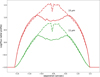 |
Fig. 8 Intensity profiles at 11 (green) and 15 μm (red) derived from DDiT+ plotted as a dashed line in the nominal case (αin = 2, αout = −6) and as a solid line for αin = 6, αout = −6. This illustrates that the forward-modeling would be sensitive to the actual dust density profile. |
8.2 Disk mass
The range of sizes we selected by fitting the ratio F15.5/F11.4 does not exclude the existence of larger grains in the disk: they would indeed not contribute significantly to the mid-IR emission, and thus, their contribution is not constrained by the MIRI measurements. However, using the millimeter fluxes measured with ALMA, we propose estimating the fraction and range of these larger grains below and then the total mass of the disk. This is an important quantity in all formation scenarii of debris disks and their evolution.
When the best grain size distribution explaining MIRI data was determined, we evaluated the corresponding mass of the disk by simply comparing the fluxes predicted by the model assuming 1 M⊕ to the observed fluxes. We found ![Mathematical equation: $\[M_{{disk }}^{s}=0.0033\]$](/articles/aa/full_html/2025/06/aa52302-24/aa52302-24-eq12.png) and 0.0051 M⊕ for silicate and graphite grains, respectively. The subscript s means that this mass only corresponds to this range of smaller grains. This value was compared to other evaluations. Kral et al. (2020) used an MCMC method to fit millimeter observations and deduced a dust mass of 0.054 ± 0.07 M⊕, which is higher by a factor 10 to 16 than our estimates, but they considereds grains with size up to 1 cm, while we used a maximum size of 10 μm. Based on millimeter data as well, Fehr et al. (2022) estimated 10 M⊕, but without detailing how they reached this value. They only mentioned the theoretical work of Krivov & Wyatt (2021), who clearly considered sizes as large as planetesimals. This explains the huge discrepancy between the two millimeter-based estimates.
and 0.0051 M⊕ for silicate and graphite grains, respectively. The subscript s means that this mass only corresponds to this range of smaller grains. This value was compared to other evaluations. Kral et al. (2020) used an MCMC method to fit millimeter observations and deduced a dust mass of 0.054 ± 0.07 M⊕, which is higher by a factor 10 to 16 than our estimates, but they considereds grains with size up to 1 cm, while we used a maximum size of 10 μm. Based on millimeter data as well, Fehr et al. (2022) estimated 10 M⊕, but without detailing how they reached this value. They only mentioned the theoretical work of Krivov & Wyatt (2021), who clearly considered sizes as large as planetesimals. This explains the huge discrepancy between the two millimeter-based estimates.
To proceed, we estimated the range of sizes that might account for the 1.27 mm fluxes observed by Kral et al. (2020) by extrapolating our results.
A first approach was to assume that the size distribution law is valid up to large grains with a size of centimeters. In this case, the mass of dust grains with a size up to 1 cm is approximately given by ![Mathematical equation: $\[M_{{disk}}^{l}=M_{{disk}}^{s}(10~000 / 10)^{0.5}\]$](/articles/aa/full_html/2025/06/aa52302-24/aa52302-24-eq13.png) , where the ratio (10 000/10) corresponds to the ratio of the largest grain sizes (1 cm and 10 μm) considered for
, where the ratio (10 000/10) corresponds to the ratio of the largest grain sizes (1 cm and 10 μm) considered for ![Mathematical equation: $\[M_{{disk}}^{l}\]$](/articles/aa/full_html/2025/06/aa52302-24/aa52302-24-eq14.png) and
and ![Mathematical equation: $\[M_{{disk}}^{s}\]$](/articles/aa/full_html/2025/06/aa52302-24/aa52302-24-eq15.png) 5, respectively. This leads to
5, respectively. This leads to ![Mathematical equation: $\[M_{disk}^{l} \sim 0.11 ~M_{\oplus}\]$](/articles/aa/full_html/2025/06/aa52302-24/aa52302-24-eq16.png) for silicate and 0.16 M⊕ for graphite grains. Because of the level of approximation used here, we considered this value as consistent with the mass of 0.054 M⊕ proposed by Kral et al. (2020), which was derived using an entirely different approach based on an MCMC estimation. The grain density we adopted is ρ = 3.50 kg m−3 for silicate. This value corresponds to bulk silicate (Kimura et al. 2003), the most likely form in a debris disk. We used 2.16 kg m−3 for graphite grains. The agreement with Kral et al. (2020) would be better with fluffy grains with a density of about half the one of bulk material. For instance, Olofsson et al. (2016) reached a better fit with the measured scattering angle in HD 61005 by changing the porosity of silicate grains. Although we obtained a reasonable consistency between our model and the various observational data sets (MIRI, ALMA, and near-IR) for silicate grains, a mixed composition of dust that would include amorphous carbon, carboneous compounds or water ice, for instance, in addition to silicate, might also lead to an acceptable agreement.
for silicate and 0.16 M⊕ for graphite grains. Because of the level of approximation used here, we considered this value as consistent with the mass of 0.054 M⊕ proposed by Kral et al. (2020), which was derived using an entirely different approach based on an MCMC estimation. The grain density we adopted is ρ = 3.50 kg m−3 for silicate. This value corresponds to bulk silicate (Kimura et al. 2003), the most likely form in a debris disk. We used 2.16 kg m−3 for graphite grains. The agreement with Kral et al. (2020) would be better with fluffy grains with a density of about half the one of bulk material. For instance, Olofsson et al. (2016) reached a better fit with the measured scattering angle in HD 61005 by changing the porosity of silicate grains. Although we obtained a reasonable consistency between our model and the various observational data sets (MIRI, ALMA, and near-IR) for silicate grains, a mixed composition of dust that would include amorphous carbon, carboneous compounds or water ice, for instance, in addition to silicate, might also lead to an acceptable agreement.
A second approach to confirm the consistency with ALMA data was to start from the flux at 1.27 mm emitted by grains up to 10 μm, as provided by our best model, and to estimate the contribution of the whole grain population up to 1 cm, that is, the population considered by Kral et al. (2020). To do this, we considered bins of an increasing grain size, up to 10 000 μm, and we assumed that the flux F1270(a) emitted by each bin characterized by size a was proportional to KoQabsa2a−3.5Δa, where Δa is the range of bin sizes, and Ko = ΣgrainsB1270(Tgrain) is the sum on all grains of size a in the disk.
Because the optical grain properties we used (Laor & Draine 1993) are limited in size to amax = 10 μm and in wavelengths to λmax = 1 mm, we had to extrapolate the values of Qabs to size up to 1 cm and to the wavelength λ0 = 1.27 mm. In both cases, simple laws give excellent approximations of Qabs. On one hand, there is a precise behavior in λ−2 for the wavelength dependence, and on the other hand, for grains larger than 10 μm, Qabs only depends upon the quantity a/λ, so that it is always possible to compute Qabs(a, λ0) = Qabs(10, a × λ0/10) for any size a > 10 μm (see Appendix A for more details).
We then obtained the dependence on a of F1270(a), the flux emitted by each bin, and computed the theoretical integrated flux at 1.27 mm emitted by the population of all grains up to a given size a, as plotted in Fig. 9. We note that for the largest grains (>1 mm), F1270(a) reaches a plateau that justifies the hypothesis that most of the flux measured by ALMA arises from grains in the 1–10 mm range. Using this plot, we then estimated the ratio of the flux predicted at 1.27 mm to the flux that is solely due to grains of size below 10 μm: We find F1270(a < 10 μm/F1270(a < 1 cm) = 0.0031 for silicate grains and 0.0127 for graphite grains. On the other hand, our best-fit model gives F1270(a < 10 μm) = 3.73 μJy (17.8 μJy) for silicate (graphite) grains, which leads to a predicted flux from the whole population of grains F1270(a < 1 cm) = 1.20 mJy (1.40 mJy). Based on the high degree of approximation made here, this quantity can also to be considered consistent with the measured ALMA flux of 0.350 mJy mentioned by Kral et al. (2020). We conclude that our model of the disk, the MIRI measurements, and the ALMA observations agree well in general. We note that the early estimates of the dust mass in HD 106906, before the detection of the extended disk in scattered light, were all lower that the estimate we propose here. For instance, Chen et al. (2005) found a lower bound of 1.2 10−4 M⊕, but this was based on simple hypotheses, such as a perfect blackbody emission (while Qabs ≈ 0.1 at 40 μm the typical wavelength of emission of 70 K grains), a grain size of ≈1 μm, and a disk with Rc = 10 au. The similar estimate by Jang-Condell et al. (2015), 1.4 × 10⁻⁴ M⊕, also relied on some currently unlikely hypotheses : Rc = 12 au, and Tgr = 108 K. Finally, Mittal et al. (2015) proposed a somewhat higher mass of 2.3 × 10⁻³ M⊕, but again assuming a very compact disk with a radius of 8 au and a rather high value of the exponent in the power-law size distribution (q = 4.16).
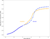 |
Fig. 9 Theoretical estimation of the flux F1270 at 1.27 mm emitted by the population of grains (silicate shown in blue, and graphite shown in orange) up to a given size a (see text). The plotted quantity is proportional to the actual physical quantity. The first thicker part of the curve covers the range of sizes (<10 μm) for which our model provides absolute values of the flux. |
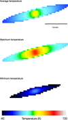 |
Fig. 10 From top to bottom: maps of the average, the maximum, and the minimum dust grain temperature along each line of sight for the nominal set of parameters with silicate grains. The color-scale covers the range 40–130 K, as indicated at the bottom. |
8.3 Dust temperature
The code DDiT+ computed the equilibrium temperature of each grain in the disk and produced a map of the average temperature along the line of sight. Fig. 10 displays this map for the nominal set of parameters and silicate grains, and the maps of the maximum and minimum temperature along the line of sight. We do not show the case of graphite grains, but the results are very similar.
The average grain temperature given by the model, considering the whole disk, is 74 K. Chen et al. (2005) derived a color temperature of 90 K from Spitzer 24 and 70 μm broadband photometry, while Bailey et al. (2014), who also used data from MIPS-SED spectra up to 100 μm found a fit by a blackbody temperature of 95 K. This is consistent with our result, considering that the actual range of grain temperatures derived from our best model is from 40 K at the edge to 130 K at the center. Along a given line of sight, the amplitude of the temperature variation is 48 K at the center and 33 K at the edge. The grain temperature is also dependent on the grain size: the smallest grains (a = 0.3 μm) have an average temperature of 93 K, and the largest grains (a = 10 μm) a temperature of 54 K. Since there is essentially no gas in the disk, and thus, no thermalization, except through very rare grain-grain collisions, this dispersion in temperature is expected to have consequences on the possible formation and segregation of ice mantles, whose condensation temperature lies in the range 40–130 K, such as methane hydrate (78 K). Water ice (180 K) or ammonia hydrate (131 K) can be present everywhere, if indeed their condensation may occur.
8.4 Other planets
While HD 106906b is well detected and will be studied in a future paper, the MIRI observations also allowed us us to estimate the limit of a detection of closer-in planets. For the sake of simplicity, we assumed only two cases, a planet located inside the disk at 0.5″, and another planet farther out at 2.5″, both aligned with the disk orientation. The image of each planet was modeled with the same numerical simulation as we used to model the disk in order to account for the coronagraph attenuation. The limits of detection were derived with the injections of simulated planets, from which we measured a star-to-planet contrast of 500 and 7000 at 0.5″ and 2.5″, respectively. This corresponds to ΔMF1140C = 6.7 and 9.6 magnitude. For the evolutionary and atmosphere model ATMO2020 (Phillips et al. 2020)6 these values translate into a mass of 15 MJup at 0.5″ and about 2–3 MJup at 2.5". The detection limits from VLT/SPHERE in Lagrange et al. (2016) did not use the same evolutionary models. Starting from their contrast measurements coupled with ATMO2020, we obtained 6 MJup and about 2–3 MJup at the same angular separations. Therefore, inside the disk, MIRI is strongly affected by the intensity of the disk and a poorer angular resolution, while both instruments achieve similar sensitivity in terms of the planet mass at larger separations.
9 Conclusions
We reported successful MIRI-JWST coronagraphic observations of the debris disk around HD 106906 at 11.4 and 15.5 μm. The disk, seen quasi edge-on, is well detected at the two wavelengths and extends in the direction observed in the near-IR, with the difference, however, that it is clearly more compact. There is some indication of a slight asymmetry between the two lobes that approximately matches the asymmetry already noted in the near-IR.
We analyzed the images using a radiative transfer code based on the open-source code DDiT (Olofsson et al. 2020), but we added several modules to produce a realistic model of the scattered and thermal emission: the wavelength-dependent optical properties of grains (silicate or graphite) (Laor & Draine 1993), the distribution of grain sizes as a−3.5, the true computation of the radiative equilibrium temperature, the realistic stellar spectrum, and the physical value of the returned fluxes. The structure of the disk in the model was controlled by a set of parameters describing the distribution of dust inside and outside a critical radius. In a second step, the images produced by the model were processed by a code that realistically simulated the whole optical path of the JWST-MIRI-coronagraph ensemble. The resulting fluxes provided by the model first demonstrated that the scattered light is totally negligible at these wavelengths and that only the thermal emission of the dust that is heated by the central binary star must be considered. Using a grid of 96 models with different sets of parameters for the structure of the disk, we showed that the observed structure is well reproduced by a disk model with a critical radius of 70 au, a shallow increasing density inside (index 2), and a steeper decrease outside (index −6). The ratio of fluxes at the two wavelengths strongly constrains the range of grain sizes that cause the mid-IR emission to be between 0.45–10 μm for silicate grains and 0.65–10 μm for graphite grains. We note that the minimum size agrees well with the values predicted by some models of the blowout phenomenon due to radiative pressure, but the difference with other estimates based on near-IR may be due to the probable separate spatial distribution of grains according to their size because mid-IR and near-IR are not sensitive to the same grains. We then derived a dust mass that causes the mid-IR emission of ≈0.0033–0.0050 M⊕ and of 0.10–0.16 M⊕ when we extrapolated this to the larger grains (up to 1 cm) that cause the millimeter emission, assuming that the law a−3.5 of the size distribution is still valid at large sizes. We showed that this estimate is well consistent with ALMA observations of the disk in terms of mass and millimeter flux.
Finally, we provided a map of the dust temperature in the disk that featured an average value of 74 K, but with a wiede range of temperature within the whole disk, from 40 to 130 K.
We note that the two types of grains we considered, silicate or graphite, can provide a view of the structure and emission of the disk that is consistent with the observations. We cannot argue on the sole basis of MIRI data in favor of one or the other composition, but we clearly favor the model based on a silicate composition. We cannot exclude, however, that a mixture of silicate and inclusions of carbonaceous material are also possible, as proposed, for instance, in Lebreton et al. (2012). Future spectroscopic observations will likely shed light on this question.
As a final remark, we wish to stress that the MIRI-JWST brings important constraints by giving us access to the 10–20 μm range. This is because the thermal emission by dust in this domain corresponds to the Wien part of Planck’s law, with an exponential behavior with respect to wavelength, and thus, a great sensitivity to the actual temperature distribution within the disk. The drawback clearly is the likewise high sensitivity to uncertainties, and this may explain our failure to reach a strictly firm conclusion on the nature of the grains or their size distribution.
Acknowledgements
We wish to thank warmly Johan Olofsson for having put on Github its DDiT code (Olofsson et al. 2020) and for his open mind when he was informed of the evolutions that we brought to the code, as explained in the text. D.R. and A.B. thank Philippe Thebault for a fruitful discussion on the mass of the disk. For the purpose of open access, the authors have applied a Creative Commons Attribution (CC BY) licence to the Author Accepted Manuscript version arising from this submission. J.P.P acknowledges financial support from the UK Science and Technology Facilities Council, and the UK Space Agency.
Appendix A Computation of Qabs at λ = 1.27 mm for grains larger than 10 μm
The optical properties of silicate that we used (Laor & Draine 1993) are limited in size to amax = 10 μm and in wavelengths to λmax = 1 mm. To extrapolate Qabs at the wavelength λ0 = 1.27 mm, we observe that for large Silicate grains the behavior of Qabs vs λ follows remarkably well a power law with exponent –2, as shown on Fig. A.1 for a few values of a and in the the range of wavelengths 250 - 1000 μm.
As regards the extrapolation of Qabs(1270) when grain size is larger than 10 μm, we show in Fig. A.2 that the hypothesis that Qabs(a, λ) depends only on the quantity 2πa/λ is already almost verified for Silicate grains of 4, 6.3 and 10 μm, so that using this result for any size larger than 10 μm is legitimate. Using then Qabs(10 μm, λ) as a template, the equation to compute Qabs for any grain larger than 10 μm becomes:
Qabs(a, λ) = Qabs(10, a × λ0/10).
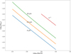 |
Fig. A.1 Behavior of Qabs vs λ in the range λ = 0.25 to 1 mm for three sizes of silicate grains : 4, 6.3 and 10 μm. |
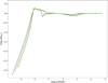 |
Fig. A.2 Behavior of Qabs vs 2πa/ λ in the range λ = 0.25 to 1 mm, for three sizes of silicate grains : 4, 6.3 and 10 μm, using the same color code as for Fig. A.1. |
Appendix B Comparison with models in worst cases
Fig. B.1 displays two cases of parameters for which the DDiT+ models provide clearly a bad fit to the observations, as compared to the best model.
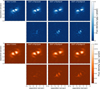 |
Fig. B.1 Comparison between observed images and DDiT+ models in cases where residues are large. The residues are below the simulated images. The first column is the observation, the second the best case, and the two last ones show, two examples of bad cases. |
Appendix C Appearance of the whole disk in the best case
Fig. C.1 displays the appearance of the best DDiT+ models at the various stages of the numerical simulations.
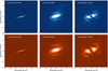 |
Fig. C.1 Illustration of the different steps of the simulation of synthetic disk images for the two filters (F1140C at the top, F1550C at the bottom). From left to right: DDiT+ disk model, non-coronagraphic image, coronagraphic image). |
Appendix D Spitzer spectrum: indication of forsterite grains?
In the IRS-Spitzer spectrum of HD106906 extracted from the CASSIS Atlas (https://cassis.sirtf.com/atlas/), we identified (circle) two emission features at 23.7 and 34.0 μm that likely are characteristic of forsterite crystalline silicate (Vandenbussche et al. 2004).
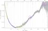 |
Fig. D.1 IRS-Spitzer spectrum of HD106906 extracted from the CASSIS Atlas (https://cassis.sirtf.com/atlas/). We marked (ovals) two emission features at 23.7 and 34.0 μm that are likely characteristic of forsterite (crystalline silicate). |
References
- Absil, O., Marion, L., Ertel, S., et al. 2021, A&A, 651, A45 [NASA ADS] [CrossRef] [EDP Sciences] [Google Scholar]
- Argyriou, I., Lage, C., Rieke, G. H., et al. 2023, A&A, 680, A96 [NASA ADS] [CrossRef] [EDP Sciences] [Google Scholar]
- Augereau, J. C., & Beust, H. 2006, A&A, 455, 987 [NASA ADS] [CrossRef] [EDP Sciences] [Google Scholar]
- Augereau, J. C., Lagrange, A. M., Mouillet, D., Papaloizou, J. C. B., & Grorod, P. A. 1999, A&A, 348, 557 [NASA ADS] [Google Scholar]
- Aumann, H. H. 1984, BAAS, 16, 483 [Google Scholar]
- Bailey, V., Meshkat, T., Reiter, M., et al. 2014, ApJ, 780, L4 [Google Scholar]
- Bhowmik, T., Boccaletti, A., Thébault, P., et al. 2019, A&A, 630, A85 [NASA ADS] [CrossRef] [EDP Sciences] [Google Scholar]
- Boccaletti, A., Lagage, P. O., Baudoz, P., et al. 2015, PASP, 127, 633 [CrossRef] [Google Scholar]
- Boccaletti, A., Cossou, C., Baudoz, P., et al. 2022, A&A, 667, A165 [NASA ADS] [CrossRef] [EDP Sciences] [Google Scholar]
- Boccaletti, A., Mâlin, M., Baudoz, P., et al. 2024, A&A, 686, A33 [NASA ADS] [CrossRef] [EDP Sciences] [Google Scholar]
- Bushouse, H., Eisenhamer, J., Dencheva, N., et al. 2025, https://doi.org/10.5281/zenodo.6984365 [Google Scholar]
- Chen, C. H., Patten, B. M., Werner, M. W., et al. 2005, ApJ, 634, 1372 [Google Scholar]
- Christiaens, V., Samland, M., Henning, T., et al. 2024, A&A, 685, L1 [NASA ADS] [CrossRef] [EDP Sciences] [Google Scholar]
- Crotts, K. A., Matthews, B. C., Esposito, T. M., et al. 2021, ApJ, 915, 58 [NASA ADS] [CrossRef] [Google Scholar]
- Debes, J. H., Weinberger, A. J., & Song, I. 2008, ApJ, 684, L41 [Google Scholar]
- De Rosa, R. J., & Kalas, P. 2019, AJ, 157, 125 [CrossRef] [Google Scholar]
- Dohnanyi, J. S. 1968, IAU Symp., 33, 486 [Google Scholar]
- Dong, R., & Dawson, R. 2016, ApJ, 825, 77 [NASA ADS] [CrossRef] [Google Scholar]
- Ertel, S., Wolf, S., & Rodmann, J. 2012, A&A, 544, A61 [NASA ADS] [CrossRef] [EDP Sciences] [Google Scholar]
- Esposito, T. M., Kalas, P., Fitzgerald, M. P., et al. 2020, AJ, 160, 24 [Google Scholar]
- Farhat, M. A., Sefilian, A. A., & Touma, J. R. 2023, MNRAS, 521, 2067 [Google Scholar]
- Fehr, A. J., Hughes, A. M., Dawson, R. I., et al. 2022, ApJ, 939, 56 [Google Scholar]
- Gaia Collaboration (Vallenari, A., et al.) 2023, A&A, 674, A1 [NASA ADS] [CrossRef] [EDP Sciences] [Google Scholar]
- Graham, J. R., Kalas, P. G., & Matthews, B. C. 2007, ApJ, 654, 595 [Google Scholar]
- Hughes, A. M., Duchêne, G., & Matthews, B. C. 2018, ARA&A, 56, 541 [Google Scholar]
- Imaz Blanco, A., Marino, S., Matrà, L., et al. 2023, MNRAS, 522, 6150 [NASA ADS] [CrossRef] [Google Scholar]
- Jang, H., Waters, R., Kaeufer, T., et al. 2024, A&A, 691, A148 [NASA ADS] [CrossRef] [EDP Sciences] [Google Scholar]
- Jang-Condell, H., Chen, C. H., Mittal, T., et al. 2015, ApJ, 808, 167 [NASA ADS] [CrossRef] [Google Scholar]
- Kalas, P. G., Rajan, A., Wang, J. J., et al. 2015, ApJ, 814, 32 [Google Scholar]
- Keppler, M., benisty, M., Müller, A., et al. 2018, A&A, 617, A44 [NASA ADS] [CrossRef] [EDP Sciences] [Google Scholar]
- Kimura, H., Mann, I., Jessberger, E. K., & Weber, I. 2003, Meteor. Planet. Sci. Suppl., 38, 5211 [Google Scholar]
- Kirchschlager, F., & Wolf, S. 2013, in Protostars and Planets VI Posters (Tucson: University of Arizona Press) [Google Scholar]
- Kral, Q., Matrà, L., Kennedy, G. M., Marino, S., & Wyatt, M. C. 2020, MNRAS, 497, 2811 [NASA ADS] [CrossRef] [Google Scholar]
- Krivov, A. V., & Wyatt, M. C. 2021, MNRAS, 500, 718 [Google Scholar]
- Lagrange, A. M., Langlois, M., Gratton, R., et al. 2016, A&A, 586, L8 [NASA ADS] [CrossRef] [EDP Sciences] [Google Scholar]
- Laor, A., & Draine, B. T. 1993, ApJ, 402, 441 [NASA ADS] [CrossRef] [Google Scholar]
- Lebreton, J., Augereau, J. C., Thi, W. F., et al. 2012, A&A, 539, A17 [NASA ADS] [CrossRef] [EDP Sciences] [Google Scholar]
- Lynch, E. M., & Lovell, J. B. 2022, MNRAS, 510, 2538 [NASA ADS] [CrossRef] [Google Scholar]
- Mâlin, M., Boccaletti, A., Baudoz, P., et al. 2024, A&A, 690, A316 [NASA ADS] [CrossRef] [EDP Sciences] [Google Scholar]
- Mathis, J. S., Rumpl, W., & Nordsieck, K. H. 1977, ApJ, 217, 425 [Google Scholar]
- Matthews, B. C., Krivov, A. V., Wyatt, M. C., Bryden, G., & Eiroa, C. 2014, Protostars and Planets VI (Tucson: University of Arizona Press), 521 [Google Scholar]
- Mazoyer, J., Boccaletti, A., Augereau, J. C., et al. 2014, A&A, 569, A29 [NASA ADS] [CrossRef] [EDP Sciences] [Google Scholar]
- Mittal, T., Chen, C. H., Jang-Condell, H., et al. 2015, ApJ, 798, 87 [Google Scholar]
- Moore, N. W. H., Li, G., Hassenzahl, L., et al. 2023, ApJ, 943, 6 [NASA ADS] [CrossRef] [Google Scholar]
- Müller, A., Keppler, M., Henning, T., et al. 2018, A&A, 617, L2 [Google Scholar]
- Nesvold, E. R., Naoz, S., & Fitzgerald, M. P. 2017, ApJ, 837, L6 [Google Scholar]
- Nguyen, M. M., De Rosa, R. J., & Kalas, P. 2021, AJ, 161, 22 [Google Scholar]
- Olofsson, J., Samland, M., Avenhaus, H., et al. 2016, A&A, 591, A108 [NASA ADS] [CrossRef] [EDP Sciences] [Google Scholar]
- Olofsson, J., Milli, J., Bayo, A., Henning, T., & Engler, N. 2020, A&A, 640, A12 [NASA ADS] [CrossRef] [EDP Sciences] [Google Scholar]
- Pan, M., Nesvold, E. R., & Kuchner, M. J. 2016, ApJ, 832, 81 [NASA ADS] [CrossRef] [Google Scholar]
- Pearce, T. D., Krivov, A. V., Sefilian, A. A., et al. 2024, MNRAS, 527, 3876 [Google Scholar]
- Pecaut, M. J., Mamajek, E. E., & Bubar, E. J. 2012, ApJ, 746, 154 [Google Scholar]
- Perotti, G., Christiaens, V., Henning, T., et al. 2023, Nature, 620, 516 [NASA ADS] [CrossRef] [Google Scholar]
- Phillips, M. W., Tremblin, P., Baraffe, I., et al. 2020, A&A, 637, A38 [NASA ADS] [CrossRef] [EDP Sciences] [Google Scholar]
- Rodet, L., Beust, H., Bonnefoy, M., et al. 2017, A&A, 602, A12 [NASA ADS] [CrossRef] [EDP Sciences] [Google Scholar]
- Rouan, D., Riaud, P., Boccaletti, A., Clénet, Y., & Labeyrie, A. 2000, PASP, 112, 1479 [Google Scholar]
- Smith, B. A., & Terrile, R. J. 1984, Science, 226, 1421 [Google Scholar]
- Strubbe, L. E., & Chiang, E. I. 2006, ApJ, 648, 652 [NASA ADS] [CrossRef] [Google Scholar]
- Thébault, P., & Augereau, J. C. 2007, A&A, 472, 169 [NASA ADS] [CrossRef] [EDP Sciences] [Google Scholar]
- Thebault, P., & Kral, Q. 2019, A&A, 626, A24 [NASA ADS] [CrossRef] [EDP Sciences] [Google Scholar]
- Vandenbussche, B., Dominik, C., Min, M., et al. 2004, A&A, 427, 519 [NASA ADS] [CrossRef] [EDP Sciences] [Google Scholar]
- Wright, G. S., Rieke, G. H., Glasse, A., et al. 2023, PASP, 135, 048003 [NASA ADS] [CrossRef] [Google Scholar]
- Wyatt, M. C. 2008, ARA&A, 46, 339 [Google Scholar]
Infrared Astronomical Satellite.
MAST: mast.stsci.edu
Available at https://github.com/joolof/DDiT
Because the mass is proportional to the integral ![Mathematical equation: $\[\int_{a_{min}}^{a_{max}} a^{3} a^{-}3.5 \mathrm{d} a= \left[a_{max }^{.5}-a_{min }^{.5}\right].\]$](/articles/aa/full_html/2025/06/aa52302-24/aa52302-24-eq17.png) .
.
Available at http://perso.ens-lyon.fr/isabelle.baraffe/ATMO2020/
All Tables
All Figures
|
Fig. 1 Top: MIRI F1140C (left) and F1550C (right) full-field coronagraphic images after data reduction (see text) and reference subtraction. The planet HD 106906 b can be seen at 7.3 arcsec NW. Bottom: same after zooming and binning by a factor 2. The orientation is standard (north is up, and east is to the left). The field of view is 22 × 22 arcsec2 at the top and 11 × 11 arcsec2 at the bottom. |
| In the text | |
|
Fig. 2 MIRI 11.4 μm coronagraphic image. The contours of the SPHERE H1-H2 image of Lagrange et al. (2016) are superimposed. |
| In the text | |
|
Fig. 3 Comparison of simulated coronagraphic images and the observed image for a few cases for which the set of parameters αin, αout, and Rc led to a rather good solution, as indicated by the low residue level (second row of each set). The two upper rows correspond to the F1140C filter, and the two bottom rows show the F1550C filter. The label at the top of each image lists the values of the parameters in short. For example, a65pi1po4 stands for Rc = 65 au, αin = 1, and αout = −4. |
| In the text | |
|
Fig. 4 Comparison of the observed coronagraphic images (left) and the best simulated images (center). The residuals of the difference are plotted at the right. |
| In the text | |
|
Fig. 5 Disk fluxes (in arbitrary units) at 15.5 μm (red) and 11.4 μm (green) emitted by each bin of grain size, as predicted by DDiT+. Only the case of silicate grains is shown here. |
| In the text | |
|
Fig. 6 Ratio Rf = F15.5/F11.4 vs. grain size for a single grain size, as given by the DDiT+ model. In blue, we show the case of silicate grains, and in orange, we show the case of graphite grains. The range of ratios deduced from observations is indicated by the shaded purple rectangle. |
| In the text | |
|
Fig. 7 Dependence of the ratio Rf = F15.5/F11.4 on the grain size distribution. The ratio Rf is deduced from the model after integration of the flux in the considered size range. Rf is plotted for a selection of different size ranges, all following a distribution in a−3.5. Each segment depicts a range that is plotted in blue for silicate grains and in orange for graphite grains. The dots correspond to single sizes of silicate grains. The two retained ranges are indicated by thicker dash-dot segments. The range of ratios deduced from observations is indicated by shaded cyan rectangle. |
| In the text | |
|
Fig. 8 Intensity profiles at 11 (green) and 15 μm (red) derived from DDiT+ plotted as a dashed line in the nominal case (αin = 2, αout = −6) and as a solid line for αin = 6, αout = −6. This illustrates that the forward-modeling would be sensitive to the actual dust density profile. |
| In the text | |
|
Fig. 9 Theoretical estimation of the flux F1270 at 1.27 mm emitted by the population of grains (silicate shown in blue, and graphite shown in orange) up to a given size a (see text). The plotted quantity is proportional to the actual physical quantity. The first thicker part of the curve covers the range of sizes (<10 μm) for which our model provides absolute values of the flux. |
| In the text | |
|
Fig. 10 From top to bottom: maps of the average, the maximum, and the minimum dust grain temperature along each line of sight for the nominal set of parameters with silicate grains. The color-scale covers the range 40–130 K, as indicated at the bottom. |
| In the text | |
|
Fig. A.1 Behavior of Qabs vs λ in the range λ = 0.25 to 1 mm for three sizes of silicate grains : 4, 6.3 and 10 μm. |
| In the text | |
|
Fig. A.2 Behavior of Qabs vs 2πa/ λ in the range λ = 0.25 to 1 mm, for three sizes of silicate grains : 4, 6.3 and 10 μm, using the same color code as for Fig. A.1. |
| In the text | |
|
Fig. B.1 Comparison between observed images and DDiT+ models in cases where residues are large. The residues are below the simulated images. The first column is the observation, the second the best case, and the two last ones show, two examples of bad cases. |
| In the text | |
|
Fig. C.1 Illustration of the different steps of the simulation of synthetic disk images for the two filters (F1140C at the top, F1550C at the bottom). From left to right: DDiT+ disk model, non-coronagraphic image, coronagraphic image). |
| In the text | |
|
Fig. D.1 IRS-Spitzer spectrum of HD106906 extracted from the CASSIS Atlas (https://cassis.sirtf.com/atlas/). We marked (ovals) two emission features at 23.7 and 34.0 μm that are likely characteristic of forsterite (crystalline silicate). |
| In the text | |
Current usage metrics show cumulative count of Article Views (full-text article views including HTML views, PDF and ePub downloads, according to the available data) and Abstracts Views on Vision4Press platform.
Data correspond to usage on the plateform after 2015. The current usage metrics is available 48-96 hours after online publication and is updated daily on week days.
Initial download of the metrics may take a while.