| Issue |
A&A
Volume 698, June 2025
|
|
|---|---|---|
| Article Number | A26 | |
| Number of page(s) | 11 | |
| Section | Stellar structure and evolution | |
| DOI | https://doi.org/10.1051/0004-6361/202451883 | |
| Published online | 29 May 2025 | |
Optical flares due to X-ray irradiation during major Be X-ray binary outbursts
1
Department of Physics, National and Kapodistrian University of Athens, University Campus Zografos, GR 15784, Athens, Greece
2
Institute of Accelerating Systems & Applications, University Campus Zografos, Athens, Greece
⋆ Corresponding author: This email address is being protected from spambots. You need JavaScript enabled to view it.
Received:
13
August
2024
Accepted:
21
March
2025
Abstract
Context. Be X-ray binaries (BeXRBs) may show strong X-ray and optical variability, and can exhibit some of the brightest outbursts that break through the Eddington limit. Major X-ray outbursts are often accompanied by strong optical flares that evolve parallel to the X-ray outburst.
Aims. Our goal is to provide a simple quantitative explanation for the optical flares with an application to a sample of the brightest outbursts of BeXRBs in the Magellanic clouds and the Galactic ULX pulsar Swift J0243.6+6124.
Methods. We constructed a numerical model to study X-ray irradiation in a BeXRB system. We then conducted a parametric investigation of the model parameters and made predictions for the intensity of the optical flares based on geometric and energetic constraints.
Results. From our modeling we found that the optical emission during major outbursts is consistent with being the result of X-ray irradiation of the Be disk. For individual systems, if this method is combined with independent constraints of the geometry of the Be disk, the binary orbital plane, and the plane of the observer, it can provide estimates of the Be disk size during major outbursts. Moreover, we computed a semi-analytical relation between optical flare luminosity and X-ray luminosity that is consistent with both model predictions and observed properties of flares.
Key words: accretion, accretion disks / stars: neutron / pulsars: general / X-rays: binaries
© The Authors 2025
 Open Access article, published by EDP Sciences, under the terms of the Creative Commons Attribution License (https://creativecommons.org/licenses/by/4.0), which permits unrestricted use, distribution, and reproduction in any medium, provided the original work is properly cited.
This article is published in open access under the Subscribe to Open model. This email address is being protected from spambots. You need JavaScript enabled to view it. to support open access publication.
1. Introduction
High-mass X-ray binaries (HMXBs) are young binary systems composed of a compact object and a massive star, and they are commonly bright in X-rays due to the large mass transfer rates. Many HMXBs have a Be star donor and are referred to as Be X-ray binaries (BeXRBs; for a review see Reig 2011). Be X-ray binaries that host neutron stars (NSs) are some of the most variable systems in the X-ray sky. Be stars are characterized by infrared excess and strong emission lines, which are highly variable in intensity and shape (Harmanec et al. 1982). It is generally accepted that these lines originate from a “decretion” disk of ejected ionized gas. Long-term variability in the optical implies a constantly evolving disk. At the same time, strong X-ray emission from BeXRBs occurs during type I and major type II outbursts. Type I X-ray outbursts (LX∼1036−1037 erg s−1) are typically periodic and occur near the periastron passage, while type II outbursts (LX≳1037 erg s−1) may last longer (sometimes multiple orbital periods) and occur once every ten years or so.
The BeXRBs are also variable in optical wavelengths. Periodic modulation on timescales of days may be related to non-radial pulsations of the Be star. Periodicity on timescales of weeks to months is often proven to be related to orbital effects, while there are a couple of highly eccentric systems that have periods of many years (e.g. Haberl et al. 2017; Petropoulou et al. 2018). However, a general feature of Be stars is long-term variability on the order of thousands of days (e.g., Kourniotis et al. 2014; Treiber et al. 2021, 2025), which can be due to disk depletion and formation events (e.g., de Wit et al. 2006) and also be associated with disk precession and truncation effects driven by the NS (Martin et al. 2011; Martin 2023).
In the era of multiwavelength astronomy, most major outbursts of BeXRBs have been monitored in the X-ray and optical. In particular, in the Magellanic Clouds (MCs), a select number of BeXRBs had type II X-ray outbursts with LX larger than 1038 erg s−1 within the last 10 years. Another great example is the major 2017 outburst of Swift J0243.6+6124, which is labeled as one of the closest ultraluminous X-ray sources (ULXs; Wilson-Hodge et al. 2018). All of these bright X-ray events are associated with strong optical flares that may not directly be related to the long-term super-orbital variability commonly seen in Be stars.
Optical variability and flares have been the focus of numerous studies in X-ray binaries revealing all sorts of intriguing phenomena. Reflection and irradiation has been studied in black hole and NS binaries (Wu et al. 2001), from milliseconds (Gandhi et al. 2010; Vincentelli et al. 2023) to longer timescales (e.g. orbital, Wu et al. 2001; Copperwheat et al. 2005). Such studies have recently been extended to multi-wavelength properties of Ultra-luminous X-ray sources (e.g. Ambrosi et al. 2022). The inclusion of a geometrical structure around Be stars adds more complexity to such modeling that is worth further investigating.
In this work, we have identified a sample of such optical flaring events in the recent literature associated with major type II outbursts (e.g. Treiber et al. 2025). To explain these optical flares quantitatively, we have constructed a numerical model that computes the irradiation effects on the Be star and the disk based on a given geometrical configuration. We present the model predictions for individual systems and how these can be combined with other independent measurements of the orbital parameters to constrain the Be disk properties. Finally, we discuss how this model predicts a linear scaling between the logarithms of the luminosities of the optical flares and X-ray luminosity and how this compares with observational data.
2. Data and sample selection
2.1. Optical data from BeXRB outbursts
Historically, multiple outbursts of BeXRBs have been observed in the optical by the Optical Gravitational Lensing Experiment (OGLE, Udalski et al. 1992, 2008, 2015, which has monitored the MCs since 1992. Since the start of OGLE-II in 1997, images have been taken at Las Campanas Observatory in the V and I bands with the 1.3 m Warsaw telescope. The subsequent phases, OGLE-III and OGLE-IV, involved instrument improved and an increased field of view. The OGLE database1 provides the light curves of most known X-ray binaries in the MCs and Udalski et al. (2008) describes the data reduction.
2.2. X-ray data from outbursts
Major outbursts in the MCs are often detected by all-sky surveys from observatories like BAT on the Neil Gehrels Swift Observatory (i.e. Swift; Gehrels et al. 2004). Follow-up observations are typically performed by Swift/XRT, NICER, or XMM-Newton in soft X-rays (0.3–10 keV). The bolometric LX is best estimated from broadband X-ray data obtained by telescopes such as NuSTAR (Harrison et al. 2013); otherwise, it may be inferred using empirical scaling relations. For type II outbursts, LX in the 0.5–10 keV band is about 40% of the bolometric LX (Anastasopoulou et al. 2022). X-ray analysis of the data is beyond the scope of this work, and we rely on data from the literature for LX estimates.
2.3. Major BeXRB outbursts
For our study, we focus on six BeXRB outbursts, from four systems located in the Small Magellanic Cloud (SMC), one in the Large Magellanic Cloud (LMC), and one Galactic system, as is presented in Table 1. Regarding our selection criteria, we searched for bright outbursts in the MCs that had a peak luminosity higher than 1038 erg s−1 and that also had available optical monitoring data via OGLE (see Sec. 2.1). For example, one of the brightest outbursts in the LMC was that of RX J0209.6−7427 (Vasilopoulos et al. 2020), but due to its location there was no OGLE coverage. The selected systems are:
-
RX J0520.5−6932 (also known as LXP 8.04): an X-ray pulsar in the LMC (Vasilopoulos et al. 2014). Its 2014 type II outburst was monitored with Swift/XRT, while two NuSTAR visits were performed (Tendulkar et al. 2014).
-
SMC X-2: Its 2015 outburst was monitored by Swift/XRT, while three NuSTAR pointings were performed (e.g. Jaisawal et al. 2023).
-
SMC X-3: Its major 2016-7 outburst was perhaps the brightest one from a pulsar in the SMC (Tsygankov et al. 2017). It was monitored by Swift/XRT, while two NuSTAR pointings were performed during the outburst.
-
SXP 4.78: The 2018 outburst of the system was monitored by Swift/XRT and NICER, showing a peak luminosity of about 7×1037 erg s−1 at 0.5–8 keV (Guillot et al. 2018), which would translate to a bolometric value of 1.8×1038 erg s−1 assuming typical correction values. No orbital period is known for the system; however, empirical relations put the period between 20 and 100 d. A single peak Hα emission line would indicate a face-on Be disk orientation (Monageng et al. 2019).
-
SXP 5.05: Coe et al. (2015) have extensively studied this intriguing system. It shows X-ray eclipses from the Be disk, indicating an almost edge-on orbital modulation. A double peak Hα emission line also indicates an edge-on disk. The X-ray luminosity of the system in the 0.5–10 keV was 0.5×1037 erg s−1, indicating a peak bolometric LX of 1.3×1038 erg s−1.
-
Swift J0243.6+6124: This source (hereafter J0243) is referred to as the Galactic ULX as it reached 1039 erg s−1 during its major 2017 outburst (Wilson-Hodge et al. 2018). Regarding its distance, many early works in the literature adopted a value of 7 kpc, while GAIA DR3 provided the updated value of 5.2 kpc (Bailer-Jones et al. 2021). A detailed orbital solution has been obtained for the system (e.g. Karaferias et al. 2023). The optical companion is a O9.5Ve star indicating a 30° inclination of the orbital plane compared to the observer (Reig et al. 2020). For the optical evolution of the outburst, we used published (Liu et al. 2022) and public data2 in the V band. For the overall evolution of J0243, we looked at the V band light curve that includes data from Liu et al. (2022) and ASAS-SN. Due to the presence of a contaminating source in the field, we introduced a 0.2 mag shift in ASAS-SN magnitudes (see Liu et al. 2022 for details about the optical data). However, for consistency in modeling the flare, we used only I-band light curves.
BeXRBs’ observed parameters.
For our sample, all optical light curves are presented in Fig. 1, while for comparison we also plot X-ray data from Swift/XRT to pinpoint the epoch of the X-ray flares. With regard to optical magnitudes, it is important to correct for extinction. For the MC systems, corrections are minimal and can be performed by using literature values for reddening, where AI≈1.5E(V−I) (Skowron et al. 2021). For J0243, we adopted an AV = 3.48 value (Reig et al. 2020) and the extinction curve of Fitzpatrick & Massa (2007) to compute AI. The values are presented in Table 1.
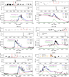 |
Fig. 1. Optical flares during major outbursts from BeXRBs. The top panels show the historic OGLE I band light curves, while the epochs of flares are marked with red boxes. The middle panels present Swift/XRT 0.3–10.0 keV light curves. Each flare (see lower panel) is fit by a model composed of a polynomial and a two-sided Gaussian. The flare amplitude from the fit is given in the label with green fonts. We also mark the I mag of the maximum flux with a vertical magenta arrow and provide the Δmag difference of that point from the polynomial background. The difference between the two maxima could be related to orbital modulation during the flares (see the cases of SXP 5.05 and LXP 8.04). |
2.4. Modeling of optical light curves
Our main goal is to model the optical light curves and measure the intensity of the optical flares. After identifying the optical flares, we performed a fit that combines a quadratic polynomial background and a two-sided Gaussian function. The flare function is expressed as:
 (1)
(1)
where tpeak is the peak time of the flare, A its amplitude in magnitude units, and σ1, 2 the rise and decay term of the flare. The above method can be used effectively for smooth flares; however, in many cases there are sharper features in the light curve that last only a few days. To study the effect of these mini-flares, we also identified the maximum of the flare and compared it with the background level estimated from the fit. Then the maximum of these mini flares is Δm=mbg−mflare. Since these flares are compared to the background, the Δm value is actually larger than A value. We note that these mini-flares are not crucial to the analysis performed from this point on, but are useful to identify the effect of noise on the data from this secondary variability on top of the major optical flares. The results of this modeling are presented in Fig. 1 and Table 2. For systems such as SXP 5.05 and LXP 8.04, there is still strong orbital modulation during the flaring period, which affects the flare shape; thus, in these cases the σ1, 2 values derived from the fit are unreliable. In any case, although we list all of the parameters from the fit, our emphasis is only on the amplitude of the flare and all other parameters should be used with caution.
BeXRBs’ optical flare parameters.
3. The irradiation model
3.1. Setup of the X-ray irradiation model
We constructed a numerical model to compute the temperature change, the change in emitted flux, and the optical magnitude of the Be Star and its surrounding decretion disk due to the X-ray irradiation from an X-ray source (i.e., the accreting NS). For the geometrical problem, we used a Be star, a Be disk, and the X-ray source placed at a distance, Rsep. We created a grid of points to map the surface of a spherical star with radius RBe as well that of a flat disk that we treated as a two-dimensional surface with inner and outer radii, Rin and Rout. The X-ray luminosity, LX, and the inclination, θNS, of the NS compared to the plane of the Be disk is also a free parameter. A θNS value of zero denotes an edge-on disk compared to the NS position, and 90 deg a face-on disk. For the non-X-ray-irradiated system, we can adopt a star temperature, T★, and a disk temperature profile that drops as a function of distance, following a typical relation:
 (2)
(2)
where Tdisk, 0 is the disk temperature at R★ and n takes typical values of −3/4 (e.g. Carciofi & Bjorkman 2006). Observational applications to BeXRB disk variability follow the above temperature profile with Tdisk, 0 = 0.9T★ (e.g. de Wit et al. 2006). However, close to the star detailed integration of non-LTE codes may yield a more complex behavior (Carciofi & Bjorkman 2006):
![Mathematical equation: $$ T_{\mathrm {disk}}(r) = \frac {T_\star }{\pi ^{1/4}} \left [ \sin ^{-1}\left (\frac {R_\star }{r} \right ) - \frac {R_\star }{r} \sqrt {1-\frac {R_\star ^2}{r^2}} \right ] ^{1/4}. $$](/articles/aa/full_html/2025/06/aa51883-24/aa51883-24-eq3.gif) (3)
(3)
The above equation provides a good agreement with simulations but can deviate for large r values or very small disk densities (see Carciofi & Bjorkman 2006 for discussion). For our problem and a typical disk configuration (i.e., r∈[1.5, 7]R★), Eqs. (2) and (3) agree for n≈0.8 and Tdisk, 0≈0.72T★. For the rest of the paper, we adopt Eq. (3).
For a particular orientation, we computed the distance of each surface element of the grid (for the Be star and the disk) from the X-ray source (dele), and the cosine of the angle between the normal of the surface element and the direction of the NS, cosϕele. Then the temperature change, ΔT, was computed from the following expression:
 (4)
(4)
where a is the albedo of the star or disk, which we assume to be 0.5, and σ is the Stefan-Boltzmann constant.
In Fig. 2, we plot three different problem setups to illustrate the geometry of the problem and the effect of irradiation. In this setup, we place the NS at a distance of Rsep∼64 R⊙ and RBe = 8 R⊙, to roughly represent systems such as LXP 8.04 and J0243. In all cases, T0 was set at 30 000 K, Rout was set at 9RBe, and the inclination angle, θNS, at 45°. From these plots, we can extract a few quantitative takeaways. The surface of the Be star is not significantly heated by irradiation, and even for 1039 erg s−1 the surface temperature only changes by ∼1–2%. Moreover, the effect of heating in the disk should be more evident, in terms of a change in magnitude, for systems in which the inner radius of the Be disk is truncated away from the Be star surface. When the inner Be disk radius touches the Be star, then even with irradiation the maximum temperature of the disk is at RBe, while when the inner Be disk radius is 2RBe, the maximum temperature after irradiation is at the point closest to the NS. We note that Be disks as large as the ones in our examples would not be dynamically stable as they would be truncated by dynamical forces.
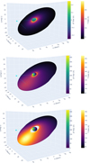 |
Fig. 2. Examples of model setup. All objects are to scale apart from the NS size (cyan color). From top to bottom, we used three different sets, for LX and Rin; [0, RBe], [1039 erg/s, RBe], and [1039 erg/s, 2RBe]. In all cases, T0 was set at 30 000 K, Rout was set at 9RBe, and the inclination at 45°. The colors indicate ΔT compared to the minimum temperature of each object element and were computed separately for disk and star for illustration purposes. If the Be disk touches the Be star surface, then its maximum temperature is at that point, regardless of irradiation or not. |
To compute the spectral energy distribution (SED) from the irradiated disk, we summed the contributions from each differential area element, ΔA, on the disk. For a face-on view, the total luminosity, Lλ, at a given wavelength, λ, was obtained by summing the specific intensities over all the elements:
 (5)
(5)
where Bλ(λ, Ti) is the Planck function at temperature Ti corresponding to the i-th element, and ΔAi is the area of the (i)-th element. The factor of π accounts for the integration over all solid angles for isotropic emission. This formulation provides the SED as observed from a viewpoint directly above the disk, assuming a face-on orientation for the observer. For the SED measured by an observer at a distance, D, we computed the flux by dividing by 4πD2 and 2πD2 for the star and disk, respectively, assuming that the disk emits only from the irradiated side.
3.2. Optical magnitudes
After computing a simulated SED (i.e., F(λ)), we need to estimate the fluxes and magnitudes in the optical filter. We focused on OGLE optical filters that include V and I pass-bands. First, we took into account the filter transmission curves (e.g., TV(λ) and TI(λ)) and camera quantum efficiency (QE(λ))3:
 (6)
(6)
and then we computed the magnitudes in the standard Johnson-Cousins systems4 (Bessell et al. 1998). An example of a theoretical SED from the Be star and disk system, and its decomposition in various spectral components is presented in Fig. 3. We note that irradiation of the Be star would only increase the temperature of ∼1% and a total increase in luminosity of less than 2%, given that only part of its surface is heated; thus, it has no effect on the SED even at high X-ray luminosity level. A final note should be on the numerical accuracy of our method. We used a grid of N×N points for the disk and star surface and experimented with grid sizes. We found that this mainly affected the peak temperature of each surface and affected the SED mostly on higher energies. For example, using N = 100 vs. N = 300 for our grid only introduced a 1–3% difference in computed luminosity in the I energy band. We thus adopted a value of N = 100 throughout this work.
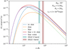 |
Fig. 3. Computed SED for a particular system configuration, similar to the ones presented in Fig. 2. Note the lower value of Rout for the Be disk to encapsulate a truncated outer disk. We plot the total SED and individual components of the star, the non-irradiated disk, and the irradiated disk. Vertical stripes mark the range of the OGLE filters. |
4. Results
4.1. Application to individual BeXRBs
We next performed simulations for individual BeXRB outbursts taking into account the orbital separation and observed LX. Regarding the optical companions of our sample, all have spectral types consistent with B1-O9, and luminosity class V, apart from SXP 4.78. Thus, their temperatures are between 26 000 and 34 000 K (Pecaut & Mamajek 2013). For simplicity, for our calculations, we adopted 30 000 K for all systems. The Be star should have a radius of 8 R⊙, similar to J0243 (Reig et al. 2020). Here, we present an application to SXP 5.05, while our results for the other systems are presented in Appendix A. Coe et al. (2015) measured the binary orbital parameters and put constraints on the Be star radius (∼5.2×1011 cm), binary separation (∼4.08×1012 cm), and Be disk size (2.6±1.8×1012 cm). Based on the eclipses, they argued for a θLOS∼83° observer line of sight compared to the normal of the orbital plane.
We constructed a two-dimensional grid of configurations for θNS and Rout, and for each grid point, we computed the change in ΔI compared to the baseline magnitude of the system (i.e., Be star and disk) in the I band. In Figs. 4, A.1 and A.2, we present heat map plots of the computed ΔI values and compare them with the observed optical flares. When compared to observed ΔI flare values (see Table 2), heat maps may be used to put a limit on the minimum disk size that would be able to reproduce these flares (see white contour lines in heat maps). As ΔI heat maps were created for a face-on observer, they represent the maximum change in color for a particular orientation, and thus assuming a moderate inclination and correcting for it, the observed flares could be a factor of 2 stronger (see black contour lines). For SXP 5.05, where θLOS∼83°, if the Be disk plane has a θNS = 23° inclination to the orbital plane, then an observer would see the Be disk with θLOS∼60°, and thus the corrected ΔI would be double the observed one. Therefore, we can infer that Rout∼0.75Rsep (see horizontal dashed line in Fig. 4) and the Be disk fills the Roche-lobe surface. We note that for the heat map in Fig. 4 we adopted a larger inner Be disk radius as otherwise the baseline luminosity of the disk would be too high to explain the flare intensity (see Fig. 4).
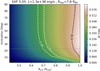 |
Fig. 4. Heat map of simulated maximum (disk is seen face on by observer) flare intensity (ΔI) for SXP 5.05 for inner disk radius RBe = 3R★. White contours indicate the observed ΔI (Table 2), while the black contour was computed assuming the disk is seen at some moderate inclination (i.e., 60°). Minimum Rout is the Be disk size and maximum should be ∼0.8Rsep, which is roughly the Roche-lobe radius. |
4.2. LX and flare intensity: Observational plane
We start with a parametric example to compare the luminosity of the irradiated disk as a function of LX. We performed simulations for a grid of parameters, computed the SED (similar to Fig. 3), and the luminosity of the optical flares in the I band, LI, as a function of the X-ray luminosity, LX. The results are plotted in Fig. 5, where we have also scaled all LI by a factor of 0.7, to account for a typical Be disk inclination compared to the observer. For low LX, the evolution is flat, indicating that the Be disk is barely heated and maintains its normal temperature. At higher LX, between 1 and 10×1038 erg s−1 we see a linear trend with a slope of ∼0.3−0.4 (depending on model parameters). At very high LX, the slope is becoming shallower toward a value of 0.25. This is consistent with the I band reaching the Rayleigh-Jeans limit as due to increasing Teff the peak of the irradiated Be disk SED shifts toward lower wavelengths. We also note the presence of a significant scatter based on just altering two main configuration parameters, θNS and Rout.
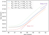 |
Fig. 5. Evolutionary tracks of optical flares luminosity as a function of LX for different model parameters. |
To compute the observational plane of LX and flare intensity, we can start with a comparison of LX and the I-band flare amplitude, A, from Table 2. This, however, has several biases, since sources have different baseline luminosity levels, and thus a Δmag of 0.2 would translate to a much different flare luminosity. Moreover, sources are at various distances, and suffer from different extinctions, effects that have already been accounted for when computing LX. The flare luminosity of each system is then computed as
 (7)
(7)
where F0, I = 112.6×10⁻¹¹ erg s−1 cm−2 Å−1 is the reference luminosity for zero mag for the I filter (∼7950 Å), and AI the correction for the I-band extinction. We plotted LI and LX in logarithmic space and proceeded to model them with a linear model including some intrinsic scatter. We used the MLFriends nested sampling MC algorithm implemented via the ULTRANEST5 package (Buchner 2021). We also introduced an excess noise term, log f, to account for the systematic scatter and noise of our data not included in the statistical uncertainties of the measurements and model. This term was added to the variance of the measurement errors as exp(2 log f). The results of the modeling are presented in Fig. 6. Interestingly, there appears to be a somehow linear relation with a slope, A, of ∼0.46 between two observed quantities and an offset, B, of 18, which is comparable to the fit onto simulated data obtained in the previous section (see Fig. 5). To further investigate this similarity, we performed model simulations for θNS∈[(5°, 90°], log(LX)∈[38, 39.5], ![Mathematical equation: $ R_{\mathrm {out}}/R_{B_{\mathrm {e}}}\in [4,9] $](/articles/aa/full_html/2025/06/aa51883-24/aa51883-24-eq8.gif) , and
, and ![Mathematical equation: $ R_{\mathrm {in}}/R_{B_{\mathrm {e}}}\in [1,2] $](/articles/aa/full_html/2025/06/aa51883-24/aa51883-24-eq9.gif) , with the results overlaid in Fig. 6.
, with the results overlaid in Fig. 6.
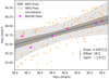 |
Fig. 6. Flare intensity as a function of log(LX), where observed data from BeXRBs are plotted with magenta colors. The best-fit line (black) and the 68–99% prediction bands are plotted with gray shade, while model parameters are given in the legend. For the modeled excess variance, we also plot an indicative spread with a maroon color, for easier comparison with the data. Orange points represent simulations for a random set of parameters (see text for details). |
Transforming the linear solution obtained from our fit to observable BeXRB data to an expression into linear space, we get:
 (8)
(8)
which provides a relation between the normalized LI, 35 and LX, 38 luminosities. The numerical factor 3 should be characteristic of I band flares, while a different scaling relation could be extracted for other optical bands.
5. Discussion
In this work, we have constructed a numerical model to study the effects of X-ray irradiation in major outbursts of BeXRB systems (see Table 1). The main free parameters of the model are the geometric configuration of the system and LX originating from the accreting NS. To investigate the validity of our model assumptions, we compared it with optical flares of six BeXRBs (see Fig. 1, and Table 2). A parametric investigation of the model indicates that in the LX range of 1–30×1039 erg s−1 that includes the brighter type II outbursts of BeXRBs, the model predicts a linear relation between LX and optical flare intensity. When compared to the observed properties of flares, the slope of the model is consistent (within errors) to the observed one, providing hints of a fundamental plane of type II outbursts and optical flares. Nevertheless, there is a significant scatter in this relation arising from model parameters like the NS-disk inclination and disk truncation. Our approach was also based on a symmetric Be decretion disk, while simulations have shown that in major outbursts the Be disks tend to become elliptic (Martin et al. 2011; Martin & Franchini 2021; Martin & Charles 2024). Moreover, there is observational evidence of warped disks during outbursts (Reig & Blinov 2018). However, qualitatively this is not an issue as in most configurations the NS would mainly illuminate one side of the disk (Fig. 2), since in our approach we compare the maximum optical intensity for a configuration that would occur at some part of the orbit when the NS illuminates the maximum possible area of the disk.
For individual systems, we can produce multiparameter contour plots and compare the max difference in I mag during a flare (ΔI) with geometrical configurations (see Figs. 4 and A.1). Interpreting ΔI heat maps can also be challenging, since we do not always know the inclination of the Be disk compared to the observer. While constraints may be put from the shape of the Hα line, at the same time, there is a degeneracy of predicted ΔI with other model parameters like Rin, as for larger Rin values the model would produce larger ΔI, as the comparison baseline would be fainter. In cases such as SXP 5.05 in which the Be disk size has been constrained from measurements of Hα lines (e.g. Coe et al. 2015, 2024), such contours are helpful as they can help to constrain the maximum disk size (Fig. 4). Regardless, there are a lot of caveats and degeneracies that can limit this approach to only qualitative discussions. For example, the baseline Be disk temperature profile may play an important role. Following Eq. (2), a sharper drop (e.g. n = 2) in temperature would result in a fainter baseline, and thus a smaller disk sizes would be required to explain an observed ΔI value. A similar effect would result from a change in the inner Be disk radius, as it would remove the hotter hart of the disk, again providing a fainter baseline luminosity. Finally, another caveat is the adoption of an albedo parameter of 0.5. It is known that soft X-rays heat up the disk surface, while hard X-rays penetrate deeper into the disk (e.g. Wu et al. 2001; Copperwheat et al. 2005), and thus accounting for the X-ray spectral shape is important. BeXRB pulsars have generally hard spectra with a cutoff and emit more than 40% of their energy below 10 keV (Anastasopoulou et al. 2022). In our approach, we used a single albedo value as a simplification of these effects. Without multiwavelength data and accurate radiative transfer implementation, it is hard to break degeneracies between the above-mentioned parameters. If we focus on SXP 5.05, a higher albedo would not be possible to explain the flare intensity with a temperature profile provided by Eq. (3). A somehow steeper temperature profile and larger inner Be disk radius would be necessary to explain the optical flares. Alternatively, one would need to introduce more complex disk geometry and perhaps an eccentric or warped Be disk (Martin & Franchini 2021).
The Be disk irradiation model may also naturally explain the color–magnitude changes in major outbursts of BeXRBs. Study of color–magnitude changes is common for X-ray binaries, for which there is strong irradiation of the donor star, and the accretion disk from X-rays emitted close to the compact object. For example, studies have been performed for the transition between the hard and soft states and its imprint as a nonthermal component seen at optical wavelengths (Kosenkov et al. 2020). Another example is the effect of irradiation in ULXs and how this can possibly induce orbital signatures (e.g. Copperwheat et al. 2005, 2006), whereby these share similarities with the orbital variability that we see in this study in the form of optical mini-flares in the OGLE data. Although a detailed investigation of these effects on BeXRB systems may be the focus of a follow-up work, we would like to offer a qualitative example. We used the V and I magnitudes from J0243 monitoring (Liu et al. 2022) and compared them to simulated color-magnitude diagrams. We followed a procedure similar to the parametric modeling that was used to create evolutionary paths shown in Fig. 5 for four sets of parameters. For all sets, we adopted Rin=RBe = 8 R⊙, an orbital separation of 12.4RBe, and we also assumed that the disk plane is inclined to the line of sight so luminosity of flares is reduced by 50%. We then experimented with star temperature and inclination, θNS, of the NS orbit compared to the Be disk. In Fig. 7, we plot the computed V and I absolute magnitudes together with extinction-corrected absolute magnitudes for J0243. Matching the data with the simulated grid was done by eye and adopting distance and extinction values within an acceptable range. We found that for a distance of 6.3 kpc and AV = 3.3 mag we get an excellent agreement within observations and data, while the results seem to favor lower θNS angles. Our investigation is partially qualitative as we treat the star as a pure blackbody and do not adopt a stellar atmosphere template. This would mainly cause the baseline point of the models (lower left in Fig. 7) to shift; however, the evolutionary tracks would remain unchanged. A few general conclusions can also be derived from this investigation. Firstly, the X-ray irradiation model may reproduce the general redder-when-brighter pattern observed in BeXRBs during outbursts. Also, as X-ray luminosity gets higher, the color changes reach a plateau, and after a critical LX around 1–10×1038 erg s−1 the color of the system becomes bluer. These characteristics are consistent with the behavior of J0243 reported by Liu et al. (2022). Interestingly, disks with sharper drops in temperature profile, or inner truncation are favored.
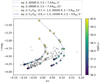 |
Fig. 7. Simulated evolutionary paths for V−I color and absolute systems magnitude of optical flares. On the plot, we overlay data for J0243 corrected for extinction (AV = 3.2 mag) and for a distance of 6.3 kpc, values selected to obtain a visual agreement to the simulated curves with temperature profiles from Eqs. (2) and (3). |
Recently, Alfonso-Garzón et al. (2024) studied the optical/UV light curves and compared them to the X-ray fluxes along the 2017 outburst of J0243. In their findings, they contribute optical/UV flare to a combination of X-ray irradiation of the Be star surface and the accretion disk. However, they overestimate the heating of the Be Star surface (see our Fig. 2), while ignoring the contribution of the Be disk irradiation6. Here, we offer a qualitative explanation for the optical flare in the 2017 outburst of J0243. While detailed modeling of the complete optical/UV light curves is beyond the scope of this work, it demonstrates the importance of X-ray irradiation of the Be disk.
Our findings would perhaps hold higher importance for the study of the population than individual sources. Possible applications would include searching archival optical data to identify similarly bright optical flares that would indirectly probe “missing” major type II outbursts from BeXRBs in the MCs or even in our Galaxy. Another interesting application would be to investigate if our findings hold at fainter optical flares perhaps associated with type I outbursts as there is a plethora of systems that show these flares with ΔI∼0.02 and LX between 1 and 10×1036 erg s−1 (Vasilopoulos et al. 2013, 2017a,b; Sturm et al. 2014). However, in these systems, the asymmetry of the disk and a variable inclination of the irradiated disk elements as a function of the orbital phase adds to the complexity of the problem.
Finally, it is interesting to explore a possible connection with ULXs (see review King et al. 2023). In particular ULXs and ULX pulsars (ULXPs) have shown optical and X-ray periodicities that are not always equal to each other, possibly due to aliasing between the binary orbital period and a superorbital period (Fürst et al. 2021). In the X-rays, the super-orbital period could be related to the precession of the accretion disk and the outflows from the accreting sources (e.g. Vasilopoulos et al. 2021; Khan et al. 2022; Fürst et al. 2023). For the irradiation of stellar companion, the binary orbit is much tighter in some ULXPs and LX is close or above 1040 erg s−1, making it an important factor compared to the sources we studied here. In a recent work, Khan & Middleton (2023) studied the X-ray, UV, and optical variability in a large sample of ULXs and they concluded that while the subset may show weakly correlated joint variability, other sources appear to display nonlinear relationships between the bands. Given that systems such as NGC 300 ULX-1 and some transient ULXs and ULXPs have properties consistent with the presence of a OBe companion (e.g. Carpano et al. 2018; Heida et al. 2019; King et al. 2023), then for the study of their optical properties the emission from an irradiated Be disk should be accounted for.
6. Conclusion
We have demonstrated how optical flares in major type II outbursts can be attributed to X-ray irradiation of the Be decretion disk by the X-ray emission of the NS. Although application to individual systems might be challenging due to multiple model parameters and degeneracies, this model yields a fundamental linear relation between the logarithms of the X-ray luminosity from the accreting NS and the maximum luminosity of the optical flares with a slope ∼0.4−0.5. The observed scatter in the optical versus X-ray luminosity plane is also naturally explained by the combination of geometrical properties such as the inclination of the orbital plane or the observer compared to the Be disk, and the size of the B disk.
Data availability
Optical data for OGLE are publicly available through X-rom project at https://ogle.astrouw.edu.pl/ogle4/xrom/xrom.html and ASAS-SN data through https://asas-sn.osu.edu/photometry/71ac277e-d7a0-5387-9385-7be7ba02931f. X-ray light-curves are available trough the Swift/XRT data products generator (Evans et al. 2007, 2009) via https://www.swift.ac.uk/user_objects/. Other X-ray and optical data were obtained from the literature and from published papers. The data and code underlying this article will be shared on reasonable request to the corresponding author. The results of our work are available in a GitHub repository https://github.com/gevas-astro/BeXRIOT. This includes: (a) the datasets (b) code for visualization of results in python and jupyter notebooks.
Acknowledgments
I thank the anonymous referee for all their comments and suggestions that helped improve the manuscript. I also thank Maria Petropoulou for fruitful discussions during this project. GV acknowledges support from the Hellenic Foundation for Research and Innovation (H.F.R.I.) through the project ASTRAPE (Project ID 7802). This work made use of data supplied by the UK Swift Science Data Centre at the University of Leicester.
OGLE XROM portal: https://ogle.astrouw.edu.pl/ogle4/xrom/xrom.html
Available through the OGLE project https://ogle.astrouw.edu.pl/main/OGLEIV/mosaic.html
Note that for zero mag calibration corrections fλ and fν are reversed in A2 table of Bessell et al. (1998).
The authors are now incorporating an irradiated, misaligned Be disk into their model. Preliminary results (Alfonso-Garzón et al. 2025) confirm that this component is essential to explain the observations.
References
- Alfonso-Garzón, J., van den Eijnden, J., Kuin, N. P. M., et al. 2024, A&A, 683, A45 [NASA ADS] [CrossRef] [EDP Sciences] [Google Scholar]
- Alfonso-Garzón, J., van den Eijnden, J., Kuin, N. P. M., et al. 2025, A&A, 697, C3 [NASA ADS] [CrossRef] [EDP Sciences] [Google Scholar]
- Ambrosi, E., Zampieri, L., Pintore, F., & Wolter, A. 2022, MNRAS, 509, 4694 [Google Scholar]
- Anastasopoulou, K., Zezas, A., Steiner, J. F., & Reig, P. 2022, MNRAS, 513, 1400 [NASA ADS] [CrossRef] [Google Scholar]
- Bailer-Jones, C. A. L., Rybizki, J., Fouesneau, M., Demleitner, M., & Andrae, R. 2021, AJ, 161, 147 [Google Scholar]
- Bessell, M. S., Castelli, F., & Plez, B. 1998, A&A, 333, 231 [NASA ADS] [Google Scholar]
- Buchner, J. 2021, The Journal of Open Source Software, 6, 3001 [NASA ADS] [CrossRef] [Google Scholar]
- Carciofi, A. C., & Bjorkman, J. E. 2006, ApJ, 639, 1081 [Google Scholar]
- Carpano, S., Haberl, F., Maitra, C., & Vasilopoulos, G. 2018, MNRAS, 476, L45 [NASA ADS] [CrossRef] [Google Scholar]
- Coe, M. J., Negueruela, I., Buckley, D. A. H., Haigh, N. J., & Laycock, S. G. T. 2001, MNRAS, 324, 623 [Google Scholar]
- Coe, M. J., Bartlett, E. S., Bird, A. J., et al. 2015, MNRAS, 447, 2387 [Google Scholar]
- Coe, M. J., Kennea, J. A., Monageng, I. M., et al. 2024, MNRAS, 528, 7115 [Google Scholar]
- Copperwheat, C., Cropper, M., Soria, R., & Wu, K. 2005, MNRAS, 362, 79 [Google Scholar]
- Copperwheat, C., Cropper, M., Soria, R., & Wu, K. 2006, in Populations of High Energy Sources in Galaxies, eds. E. J. A. Meurs, & G. Fabbiano, IAU Symp., 230, 300 [Google Scholar]
- de Wit, W. J., Lamers, H. J. G. L. M., Marquette, J. B., & Beaulieu, J. P. 2006, A&A, 456, 1027 [NASA ADS] [CrossRef] [EDP Sciences] [Google Scholar]
- Evans, P. A., Beardmore, A. P., Page, K. L., et al. 2007, A&A, 469, 379 [NASA ADS] [CrossRef] [EDP Sciences] [Google Scholar]
- Evans, P. A., Beardmore, A. P., Page, K. L., et al. 2009, MNRAS, 397, 1177 [Google Scholar]
- Fitzpatrick, E. L., & Massa, D. 2007, ApJ, 663, 320 [Google Scholar]
- Fürst, F., Walton, D. J., Heida, M., et al. 2021, A&A, 651, A75 [NASA ADS] [CrossRef] [EDP Sciences] [Google Scholar]
- Fürst, F., Walton, D. J., Israel, G. L., et al. 2023, A&A, 672, A140 [NASA ADS] [CrossRef] [EDP Sciences] [Google Scholar]
- Gandhi, P., Dhillon, V. S., Durant, M., et al. 2010, MNRAS, 407, 2166 [NASA ADS] [CrossRef] [Google Scholar]
- Gehrels, N., Chincarini, G., Giommi, P., et al. 2004, ApJ, 611, 1005 [Google Scholar]
- Guillot, S., Vasilopoulos, G., Pasham, D., et al. 2018, ATel, 12219, 1 [Google Scholar]
- Haberl, F., Israel, G. L., Rodriguez Castillo, G. A., et al. 2017, A&A, 598, A69 [NASA ADS] [CrossRef] [EDP Sciences] [Google Scholar]
- Harmanec, P., Horn, J., & Koubsky, P. 1982, in Be Stars, eds. M. Jaschek, & H. G. Groth, 98, 269 [Google Scholar]
- Harrison, F. A., Craig, W. W., Christensen, F. E., et al. 2013, ApJ, 770, 103 [Google Scholar]
- Heida, M., Lau, R. M., Davies, B., et al. 2019, ApJ, 883, L34 [NASA ADS] [CrossRef] [Google Scholar]
- Jaisawal, G. K., Vasilopoulos, G., Naik, S., et al. 2023, MNRAS, 521, 3951 [Google Scholar]
- Karaferias, A. S., Vasilopoulos, G., Petropoulou, M., et al. 2023, MNRAS, 520, 281 [NASA ADS] [CrossRef] [Google Scholar]
- Khan, N., & Middleton, M. J. 2023, MNRAS, 524, 4302 [Google Scholar]
- Khan, N., Middleton, M. J., Wiktorowicz, G., et al. 2022, MNRAS, 509, 2493 [NASA ADS] [Google Scholar]
- King, A., Lasota, J. -P., & Middleton, M. 2023, New Astron. Rev., 96, 101672 [CrossRef] [Google Scholar]
- Kosenkov, I. A., Veledina, A., Suleimanov, V. F., & Poutanen, J. 2020, A&A, 638, A127 [NASA ADS] [CrossRef] [EDP Sciences] [Google Scholar]
- Kourniotis, M., Bonanos, A. Z., Soszyński, I., et al. 2014, A&A, 562, A125 [NASA ADS] [CrossRef] [EDP Sciences] [Google Scholar]
- Liu, W., Yan, J., Reig, P., et al. 2022, A&A, 666, A110 [NASA ADS] [CrossRef] [EDP Sciences] [Google Scholar]
- Maravelias, G., Antoniou, V., Zezas, A., et al. 2018, ATel, 12224, 1 [Google Scholar]
- Martin, R. G. 2023, MNRAS, 523, L75 [NASA ADS] [CrossRef] [Google Scholar]
- Martin, R. G., & Charles, P. A. 2024, MNRAS, 528, L59 [Google Scholar]
- Martin, R. G., & Franchini, A. 2021, ApJ, 922, L37 [NASA ADS] [CrossRef] [Google Scholar]
- Martin, R. G., Pringle, J. E., Tout, C. A., & Lubow, S. H. 2011, MNRAS, 416, 2827 [NASA ADS] [CrossRef] [Google Scholar]
- McBride, V. A., Coe, M. J., Negueruela, I., Schurch, M. P. E., & McGowan, K. E. 2008, MNRAS, 388, 1198 [NASA ADS] [CrossRef] [Google Scholar]
- Monageng, I. M., Coe, M. J., Townsend, L. J., et al. 2019, MNRAS, 485, 4617 [Google Scholar]
- Pecaut, M. J., & Mamajek, E. E. 2013, ApJS, 208, 9 [Google Scholar]
- Petropoulou, M., Vasilopoulos, G., Christie, I. M., Giannios, D., & Coe, M. J. 2018, MNRAS, 474, L22 [NASA ADS] [CrossRef] [Google Scholar]
- Reig, P. 2011, Ap&SS, 332, 1 [Google Scholar]
- Reig, P., & Blinov, D. 2018, A&A, 619, A19 [NASA ADS] [CrossRef] [EDP Sciences] [Google Scholar]
- Reig, P., Fabregat, J., & Alfonso-Garzón, J. 2020, A&A, 640, A35 [NASA ADS] [CrossRef] [EDP Sciences] [Google Scholar]
- Skowron, D. M., Skowron, J., Udalski, A., et al. 2021, ApJS, 252, 23 [Google Scholar]
- Sturm, R., Haberl, F., Vasilopoulos, G., et al. 2014, MNRAS, 444, 3571 [NASA ADS] [CrossRef] [Google Scholar]
- Tendulkar, S. P., Fürst, F., Pottschmidt, K., et al. 2014, ApJ, 795, 154 [Google Scholar]
- Townsend, L. J., Coe, M. J., Corbet, R. H. D., & Hill, A. B. 2011, MNRAS, 416, 1556 [NASA ADS] [CrossRef] [Google Scholar]
- Treiber, H., Vasilopoulos, G., Bailyn, C. D., et al. 2021, MNRAS, 503, 6187 [CrossRef] [Google Scholar]
- Treiber, H., Vasilopoulos, G., Bailyn, C. D., Haberl, F., & Udalski, A. 2025, A&A, 694, A43 [NASA ADS] [CrossRef] [EDP Sciences] [Google Scholar]
- Tsygankov, S. S., Doroshenko, V., Lutovinov, A. A., Mushtukov, A. A., & Poutanen, J. 2017, A&A, 605, A39 [NASA ADS] [CrossRef] [EDP Sciences] [Google Scholar]
- Udalski, A., Szymanski, M., Kaluzny, J., Kubiak, M., & Mateo, M. 1992, Acta Astron., 42, 253 [NASA ADS] [Google Scholar]
- Udalski, A., Szymanski, M. K., Soszynski, I., & Poleski, R. 2008, Acta Astron., 58, 69 [NASA ADS] [Google Scholar]
- Udalski, A., Szymański, M. K., & Szymański, G. 2015, Acta Astron., 65, 1 [NASA ADS] [Google Scholar]
- Vasilopoulos, G., Maggi, P., Haberl, F., et al. 2013, A&A, 558, A74 [NASA ADS] [CrossRef] [EDP Sciences] [Google Scholar]
- Vasilopoulos, G., Haberl, F., Sturm, R., Maggi, P., & Udalski, A. 2014, A&A, 567, A129 [NASA ADS] [CrossRef] [EDP Sciences] [Google Scholar]
- Vasilopoulos, G., Haberl, F., & Maggi, P. 2017a, MNRAS, 470, 1971 [NASA ADS] [CrossRef] [Google Scholar]
- Vasilopoulos, G., Zezas, A., Antoniou, V., & Haberl, F. 2017b, MNRAS, 470, 4354 [NASA ADS] [CrossRef] [Google Scholar]
- Vasilopoulos, G., Ray, P. S., Gendreau, K. C., et al. 2020, MNRAS, 494, 5350 [NASA ADS] [CrossRef] [Google Scholar]
- Vasilopoulos, G., Koliopanos, F., Haberl, F., et al. 2021, ApJ, 909, 50 [Google Scholar]
- Vincentelli, F. M., Neilsen, J., Tetarenko, A. J., et al. 2023, Nature, 615, 45 [Google Scholar]
- Wilson-Hodge, C. A., Malacaria, C., Jenke, P. A., et al. 2018, ApJ, 863, 9 [Google Scholar]
- Wu, K., Soria, R., Hunstead, R. W., & Johnston, H. M. 2001, MNRAS, 320, 177 [NASA ADS] [CrossRef] [Google Scholar]
Appendix A: Individual BeXRB flares: Model contour plots
Here we present heat maps (Fig. A.1) for all remaining BeXRB flares. For our calculations we adopt 30000oK and 8R⊙ for all systems. For binary separation reasonable separation values would be between 1-2a sin i if an orbital solution is available. For J0243 to be consistent with the literature we adopt 2a sin i (Reig et al. 2020). For other systems with known orbital solutions we adopt an a sin i while using the literature values from Table 1, while for SXP 4.78 we use an conservative separation of 100 ls.
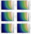 |
Fig. A.1. Heat map of simulated maximum (disk is seen face on by observer) flare intensity (ΔI) for parameters of BeXRBs of Table 1 (see text for details), with a temperature profile of Eq. 3 and inner disk radius equal to the Be star radius. White contours indicate the observed ΔI (Table 2), while black contour are corrected assuming the disk is seen by some moderate inclination (i.e. 60°). Minimum Rout is the Be disk size and maximum should be ∼0.8Rsep which is roughly the Roche-lobe. |
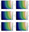 |
Fig. A.2. Same as Fig. A.1, but for a steep temperature profile (n = 2, Tdisk, 0=T★ in Eq. 2). All the contours are shifted to the left compared to Fig. A.1. |
For comparison we also perform the same heat maps using a temperature profile described in Eq. 2, with n = 2, Tdisk, 0=T★.
All Tables
All Figures
|
Fig. 1. Optical flares during major outbursts from BeXRBs. The top panels show the historic OGLE I band light curves, while the epochs of flares are marked with red boxes. The middle panels present Swift/XRT 0.3–10.0 keV light curves. Each flare (see lower panel) is fit by a model composed of a polynomial and a two-sided Gaussian. The flare amplitude from the fit is given in the label with green fonts. We also mark the I mag of the maximum flux with a vertical magenta arrow and provide the Δmag difference of that point from the polynomial background. The difference between the two maxima could be related to orbital modulation during the flares (see the cases of SXP 5.05 and LXP 8.04). |
| In the text | |
|
Fig. 2. Examples of model setup. All objects are to scale apart from the NS size (cyan color). From top to bottom, we used three different sets, for LX and Rin; [0, RBe], [1039 erg/s, RBe], and [1039 erg/s, 2RBe]. In all cases, T0 was set at 30 000 K, Rout was set at 9RBe, and the inclination at 45°. The colors indicate ΔT compared to the minimum temperature of each object element and were computed separately for disk and star for illustration purposes. If the Be disk touches the Be star surface, then its maximum temperature is at that point, regardless of irradiation or not. |
| In the text | |
|
Fig. 3. Computed SED for a particular system configuration, similar to the ones presented in Fig. 2. Note the lower value of Rout for the Be disk to encapsulate a truncated outer disk. We plot the total SED and individual components of the star, the non-irradiated disk, and the irradiated disk. Vertical stripes mark the range of the OGLE filters. |
| In the text | |
|
Fig. 4. Heat map of simulated maximum (disk is seen face on by observer) flare intensity (ΔI) for SXP 5.05 for inner disk radius RBe = 3R★. White contours indicate the observed ΔI (Table 2), while the black contour was computed assuming the disk is seen at some moderate inclination (i.e., 60°). Minimum Rout is the Be disk size and maximum should be ∼0.8Rsep, which is roughly the Roche-lobe radius. |
| In the text | |
|
Fig. 5. Evolutionary tracks of optical flares luminosity as a function of LX for different model parameters. |
| In the text | |
|
Fig. 6. Flare intensity as a function of log(LX), where observed data from BeXRBs are plotted with magenta colors. The best-fit line (black) and the 68–99% prediction bands are plotted with gray shade, while model parameters are given in the legend. For the modeled excess variance, we also plot an indicative spread with a maroon color, for easier comparison with the data. Orange points represent simulations for a random set of parameters (see text for details). |
| In the text | |
|
Fig. 7. Simulated evolutionary paths for V−I color and absolute systems magnitude of optical flares. On the plot, we overlay data for J0243 corrected for extinction (AV = 3.2 mag) and for a distance of 6.3 kpc, values selected to obtain a visual agreement to the simulated curves with temperature profiles from Eqs. (2) and (3). |
| In the text | |
|
Fig. A.1. Heat map of simulated maximum (disk is seen face on by observer) flare intensity (ΔI) for parameters of BeXRBs of Table 1 (see text for details), with a temperature profile of Eq. 3 and inner disk radius equal to the Be star radius. White contours indicate the observed ΔI (Table 2), while black contour are corrected assuming the disk is seen by some moderate inclination (i.e. 60°). Minimum Rout is the Be disk size and maximum should be ∼0.8Rsep which is roughly the Roche-lobe. |
| In the text | |
|
Fig. A.2. Same as Fig. A.1, but for a steep temperature profile (n = 2, Tdisk, 0=T★ in Eq. 2). All the contours are shifted to the left compared to Fig. A.1. |
| In the text | |
Current usage metrics show cumulative count of Article Views (full-text article views including HTML views, PDF and ePub downloads, according to the available data) and Abstracts Views on Vision4Press platform.
Data correspond to usage on the plateform after 2015. The current usage metrics is available 48-96 hours after online publication and is updated daily on week days.
Initial download of the metrics may take a while.