| Issue |
A&A
Volume 664, August 2022
|
|
|---|---|---|
| Article Number | A194 | |
| Number of page(s) | 12 | |
| Section | Extragalactic astronomy | |
| DOI | https://doi.org/10.1051/0004-6361/202243909 | |
| Published online | 30 August 2022 | |
X-ray view of the 2021 outburst of SXP 15.6: Constraints on the binary orbit and magnetic field of the neutron star
1
Université de Strasbourg, CNRS, Observatoire astronomique de Strasbourg, UMR 7550, 67000 Strasbourg, France
e-mail: This email address is being protected from spambots. You need JavaScript enabled to view it.
2
National Space Institute, Technical University of Denmark, Elektrovej 327-328, 2800 Lyngby, Denmark
3
Max-Planck-Institut für extraterrestrische Physik, Gießenbachstraße 1, 85748 Garching, Germany
4
Department of Physics, National and Kapodistrian University of Athens, University Campus Zografos, 15783, Athens, Greece
Received:
28
April
2022
Accepted:
13
June
2022
Abstract
Aims. We conducted a spectral and temporal analysis of X-ray data from the Be X-ray binary pulsar SXP 15.6 located in the Small Magellanic Cloud based on NuSTAR, NICER, and Swift observations during the 2021 outburst.
Methods. We present the broadband X-ray spectra of the system based on simultaneous NuSTAR and NICER observations for the first time. Moreover, we used monitoring data to study the spectral and temporal properties of the system during the outburst.
Results. Comparison of the evolution of the 2021 outburst with archival data reveals a consistent pattern of variability, with multiple peaks occurring at time intervals similar to the orbital period of the system (∼36 d). Our spectral analysis indicates that most of the energy is released at high energies above 10 keV, while we found no cyclotron absorption line in the spectrum. Analysing of the spectral evolution during the outburst, we find that the spectrum is softer when brighter, which in turn reveals that the system is probably in the super-critical regime in which the accretion column is formed. This places an upper limit on the magnetic field of the system of about 7 × 10¹¹ G. The spin-evolution of the neutron star (NS) during the outburst is consistent with an NS with a low magnetic field (∼5 × 10¹¹ G), while there is evident orbital modulation that we modelled, and we derived the orbital parameters. We found the orbit to have a moderate eccentricity of ∼0.3. Our estimates of the magnetic field are consistent with the lack of an electron cyclotron resonance scattering feature in the broadband X-ray spectrum.
Key words: stars: neutron / X-rays: individuals: SXP 15.6 / Magellanic Clouds / X-rays: binaries
© G. Vasilopoulos et al. 2022
 Open Access article, published by EDP Sciences, under the terms of the Creative Commons Attribution License (https://creativecommons.org/licenses/by/4.0), which permits unrestricted use, distribution, and reproduction in any medium, provided the original work is properly cited.
This article is published in open access under the Subscribe-to-Open model. This email address is being protected from spambots. You need JavaScript enabled to view it. to support open access publication.
1. Introduction
Accreting X-ray pulsars (XRPs) in high-mass X-ray binaries (HMXBs) are of key importance in the study of accretion and binary evolution. The majority of XRPs are found in the so-called Be X-ray binaries (BeXRBs; see Reig 2011, for a review), where mass transfer from the donor to the neutron star (NS) occurs through a slow-moving equatorial disk (i.e., decretion disk). A plethora of information about the physical properties of the systems may be acquired during outburst. Type I outbursts occur during the NS periastron passage, while major outbursts with an X-ray luminosity LX > 1037 erg s−1 are quite rare and occur on timescales of years to decades (Okazaki et al. 2013; Martin et al. 2014; Martin & Franchini 2021). These rare outbursts enable the study of the broadband X-ray spectral shape and the search for cyclotron resonant scattering features (CRSFs), which offer the only tool for directly measuring the magnetic field at the NS surface. During outbursts, such systems have been found to show both evolution in the continuum spectra and – in some cases – CRSFs (Jaisawal & Naik 2016; Maitra et al. 2018; Staubert et al. 2019), yielding diagnostic data for the state of accretion (Becker & Wolff 2007; Becker et al. 2012; Postnov et al. 2015). Although the Magellanic Clouds (MCs), especially the Small Magellanic Cloud (SMC), are populous in BeXRBs (Haberl & Sturm 2016), the presence of a CRSF is known only for a handful of systems, mainly owing to the lack of coverage in the hard X-ray band during its bright state. Moreover, X-ray pulsars in the MCs offer quite favourable conditions as they are placed at known distances (in contrast to most Galactic systems) and have only low Galactic absorption. This allows a precise determination of their luminosities. In addition, the knowledge of the spin period and the magnetic field is crucial for constraining the accretion torque models and examine whether most of the BeXRBs are in spin equilibrium. Even if the magnetic field cannot be directly measured via CRSF, the study of the spin evolution can deliver constraints or indirect estimates of the magnetic field of the NS.
SXP 15.6 (also known as XMMU J004855.5−734946) is a BeXRB pulsar in the SMC (Vasilopoulos et al. 2017b). The orbital period of the system has been proposed to be 36.432 d based on optical monitoring data from OGLE (McBride et al. 2017), while a more recent analysis of OGLE data derived an optical period of 36.411 d (Coe et al. 2022). The spin period of the NS was detected in 2016 from Chandra observations, and since then, no further strong outburst was witnessed until 2021. On 2021 November 19, a strong outburst was detected by Swift/XRT (Coe et al. 2021) at a luminosity level of 2 × 1037 erg s−1 (0.3–10 keV) for a distance of 62 kpc (Graczyk et al. 2014). Follow-up NICER and NuSTAR target of opportunity (ToO) observations enabled us to study the spin evolution of the NS as well as its broadband spectral properties. Based on these data, we report estimates of the fundamental properties of the system such as the orbital parameters and the magnetic field of the NS.
2. X-ray view of SXP 15.6
2.1. 2021 outburst
The 2021 outburst of SXP 15.6 was reported by Coe et al. (2021) as a result of monitoring from the Swift SMC Survey (S-CUBED; Kennea et al. 2018). S-CUBED is a high-cadence (one to two weeks) shallow X-ray survey of the SMC that consists of ∼140 tiled pointings covering the optical extent of the SMC. The survey has enabled the early detection of some of the brightest outbursts in the MCs (e.g., SMC X-3; Kennea et al. 2016). Following the announcement of the outburst, NICER monitoring observations were performed, while NuSTAR observed the system near its peak flux with a ToO observation. In the following paragraphs we provide information for the NICER and NuSTAR data that were collected during the outburst, as well as Chandra archival data that were used for comparative studies.
2.2. Data analysis
2.2.1. NuSTAR
The Nuclear Spectroscopic Telescope Array (NuSTAR) mission carries the first focusing high-energy X-ray telescope in orbit operating in the band from 3 to 79 keV (Harrison et al. 2013). NuSTAR observed the system with a 42 ks DDT observation (obsid: 90701339002) on 2019 November 26 (MJD 59544.40−59545.25). NuSTAR data were analysed with version 1.8.0 of the NuSTAR data analysis software (DAS) and instrumental calibration files from CalDB v20220301. The data were calibrated using the standard settings on the NUPIPELINE script, reducing internal high-energy background, and screening for passages through the South Atlantic Anomaly. We used the NUPRODUCTS script to extract phase-averaged spectra for source and background regions (60″ radius) for each of the two focal plane modules (FPMA/B). Finally, we performed barycentric corrections to the event times of arrival using the satellite’s orbital ephemeris files.
2.2.2. NICER
The NICER X-ray Timing Instrument (XTI; Gendreau et al. 2012, 2016) is a non-imaging, soft X-ray telescope on board the International Space Station. The XTI consists of an array of 56 co-aligned concentrator optics (52 currently active) with a field of view of ∼30 arcmin2 in the sky. Each unit is associated with a silicon drift detector (Prigozhin et al. 2012), operating in the 0.2–12 keV band, yielding a ∼100 ns time resolution and spectral resolution of ∼85 eV at 1 keV.
For the current study, we analysed NICER data obtained between MJD 59535 and MJD 59605. Data were reduced using HEASOFT version 6.29, NICER DAS version 2020-04-23_V007a, and the calibration database (CALDB) version v20210707. For the analysis, we selected good-time intervals with the nimaketime script using standard options. After inspecting the resulting light curves in different bands, we identified increased flaring activity due to background contamination. To mitigate the effects of the background, we altered some of the standard filtering parameters. We opted for ISS not in the South Atlantic Anomaly region, a source elevation > 15° above the Earth limb (> 30° above the bright Earth), and a magnetic cut-off rigidity (COR_SAX) > 2.0 GeV c−1. Unfortunately, a large fraction of the obtained data – especially during the lower flux states – was not useful due to enhanced background activity during the monitoring period and was filtered out. Finally, for the timing analysis, we performed barycentric corrections to the event times of arrival using the barycorr tool and the JPL DE405 planetary ephemeris.
Because NICER is not an imaging instrument, the X-ray background is calculated indirectly. For systems in the direction of the MCs, the 3C50 tool (Remillard et al. 2022) method is optimal (see Treiber et al. 2021). This approach uses a number of background proxies in the NICER data to define the basis states of the background database.
2.2.3. Swift
X-ray monitoring observations of SXP 15.6 have been obtained by the Neil Gehrels Swift Observatory (Swift; Gehrels et al. 2004) X-ray Telescope (XRT; Burrows et al. 2005). All archival XRT data were retrieved though the UK Swift science data centre1 and were analysed using standard procedures (Evans et al. 2007, 2009).
2.2.4. Chandra
SXP 15.6 was observed by Chandra (obsid:18885) in July 2016 (MJD 57575.34) with an exposure time of 25 ks. Analysis of these data has revealed the presence of a single-peaked pulse profile at LX = 4 × 1036 erg s−1 in the 0.3–10.0 keV band (Vasilopoulos et al. 2017b). In the current study, we used the same data to create pulse profiles for comparison with the pulse profiles during the 2021 outburst. Data reduction was performed with the CIAO v4.13 software (Fruscione et al. 2006) using standard options through chandra_repro script. Source events were extracted from a 5″ region.
3. Results
3.1. Broadband spectral properties
Spectral analysis was performed using XSPEC v12.10.1f (Arnaud 1996). Photoelectric absorption by the interstellar gas was modelled by the tbabs component in XSPEC, with solar abundances set according to Wilms et al. (2000) and atomic cross sections from Verner et al. (1996). To fit the NICER spectra, we used PG-statistics, which implements Cash-statistics (Cash 1979), with a non-Poisson background model. For the modelling of NuSTAR spectra (3.0–78 keV), we used Cash-statistics. We note that NuSTAR spectra are dominated by background above 40 keV and thus lack the sensitivity to detect faint features at high energies.
It is typical for BeXRBs in the MCs to model the X-ray absorption with a combination of two components to account for Galactic absorption and intrinsic absorption within the SMC and around the binary (e.g., Vasilopoulos et al. 2013, 2016, 2017a). The first component was fixed to the Galactic foreground value of 4 × 1020 cm−1 (Dickey & Lockman 1990). The second component was left free to account for the absorption near the source or within the SMC, thus elemental abundances were fixed at 0.2 solar (Russell & Dopita 1992). In the spectral modelling, we determine whether there is evidence of absorption in addition to the Galactic absorption.
In BeXRBs, hard X-ray spectra originate from the accretion column and can be fitted by a phenomenological power-law-like shape with an exponential high-energy cut-off above (or of about) 10 keV (e.g., Müller et al. 2013; Sturm et al. 2014; Jaisawal et al. 2018; Vasilopoulos et al. 2020). In many cases, BeXRB spectra show residuals at soft energies. These residuals are often referred to as a ‘soft-excess’ with a physical origin that is attributed to one mechanism or a combination of mechanisms such as emission from the accretion disk, emission from the NS surface, hot plasma around the magnetosphere, or partial absorption from material around the NS (Hickox et al. 2004). In this study we investigate the broadband spectrum for signatures of these mechanisms.
NuSTAR data were obtained quasi-simultaneously (i.e., less than a day apart) with two NICER visits (obsid: 4202430107 and 4202430108). An absorbed cut-off power-law model sufficiently describes the NuSTAR spectrum. However, fitting the combined NICER and NuSTAR data, we see significant structure in the residuals caused by the soft excess (see Fig. 1). To eliminate the residual structure, we need to add either a partially covering absorber or a soft thermal component to the model (see the lower panels in Fig. 1). For the thermal component, we used a disk blackbody (diskbb in XSPEC). We also included a model with a combined partial coverage on a continuum composed of a cut-off power law and a thermal component. In all our tests, the column density of the SMC intrinsic absorption was unconstrained and tends to zero. For the partial covering model, the Tuebingen-Boulder ISM model (tbpcf in xspec) only provided spectral multiplicative components for standard solar abundances because a first-order approximation for the SMC abundance NH values obtained by this model should be increased by a factor of ∼5 compared to Galactic ones. The best-fit parameters of all tested models are shown in Table 1. Based on the derived parameters, we also computed the mass-accretion rate corresponding to the bolometric luminosity by assuming that all gravitational energy is converted into radiation2 (e.g., Campana et al. 2018; Frank et al. 2002). We note that for all the tested models, the best fit yields an acceptable fit statistics with a reduced χ2 lower than one. To estimate the uncertainties, we implemented a Markov chain Monte Carlo (MCMC) model through XSPEC. We used the Goodman–Weare algorithm with 20 walkers and a total length of 50 000. For the initial burn-in phase, we needed 30 000 steps before the chain reached equilibrium. We then generated parameter errors (90% confidence) based on the chain values. To further test the goodness of the fit, we also simulated spectra based on the MCMC chain parameters. We found that for all except for the simplest models (i.e., absorbed cut-off power law), only a small number of the simulated spectra had a better fit statistics than the real spectra. Thus we should be at the limit of our capabilities in testing more complicated spectral models. We finally note that we found no evidence of an Fe Kα line in the spectrum nor any broad absorption feature that is consistent with a CRSF.
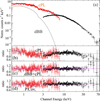 |
Fig. 1. Broadband spectrum of SXP 15.6. NuSTAR spectra are shown in black, and two NICER snapshots are shown in red and cyan. The upper panel presents the best-fit model composed of an absorbed cut-off power law and a soft thermal component. The ratio plots show the comparison of the tested models and the data: (b) Absorbed cut-off power law, (c) absorbed cut-off power law plus disk blackbody, and (d) cut-off power law with partial coverage. The model parameters are listed in Table 1. |
Best-fit parameters of the spectral empirical models.
3.2. Long-term light curves and outburst evolution
Monitoring data in the soft X-ray band with NICER enables us to study the evolution of the 2021 outburst and to compare it with Chandra data from 2016. NICER monitoring data are of sufficient statistical quality to allow us to extract enough counts and perform spectral modelling. The typical Swift/XRT exposure within one day is about 1000–2000 s, but the effective area of the detector is significantly smaller than that of NICER. Thus we used XRT data to only estimate average count rates for each XRT data set.
The 20 individual NICER spectra were fitted with an empirical absorbed power-law model in the 0.5–8 keV band. We also attempted to fit the spectra with a power law with a cut-off, but the cut-off always converged to very high values (i.e., above 100 keV). This was expected because the cut-off seen in the broad spectra is well above the upper bound of NICER spectra. For the spectral modelling, we used two absorption components as described above. We found the absorption to be consistent with the fixed foreground value of 4 × 1020 cm−1, while the power-law photon index had a mean value of Γ = 0.97, with evidence of the spectrum becoming softer when brighter at the brightest phase of the outburst. In Fig. 2 we plot the evolution of the spectral parameters and the flux for a 40-day interval (only one observation exists after MJD 59580).
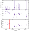 |
Fig. 2. Spectral results of NICER monitoring data obtained during the 2021 outburst of SXP 15.6. The bottom panel shows the unabsorbed flux computed in the 0.3–10.0 keV band. The red shaded region indicates the epoch of the NuSTAR ToO. No strong evidence for a change in the column density of the absorbing material (top panel) is seen, but we found evidence of spectral evolution at higher fluxes with the spectral shape (characterised by Γ, middle panel) becoming softer when brighter above 2× 10⁻¹¹ erg cm−2 s−1 (0.3–10.0 keV). |
After analysing the NICER and Swift/XRT monitoring data as well as the broadband spectra, we computed the evolution of the bolometric luminosity during the 2021 outburst and compared it with archival data. We converted the XRT count rates into 0.3–10.0 keV fluxes using the average spectral parameters inferred from the NICER spectral fits. A conversion factor of 3.16 × 1037 erg cm−2 s−1/(c/s) was used for all XRT data, while errors were estimated based on the count rate uncertainties. The broadband unabsorbed LX was estimated from the broadband spectra. Most of the energy is emitted above 10 keV because the ratio of the broadband (0.3–80 keV) to narrow band (0.3–10.0 keV) luminosity was ∼3.5. The 2021 X-ray light curve is shown in Fig. 3. In the same figure we overplot the 2016 XRT monitoring data, time-shifted so that the main peaks of each outburst match.
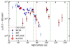 |
Fig. 3. X-ray light curves of the 2016 and 2021 outbursts. Luminosities are absorption corrected (0.3–80.0 keV) and computed for the SMC distance. Archival data from 2016 (first point at MJD 57547) are shifted in time to match the 2021 luminosity peaks. Vertical green lines mark the 36.411 d optical period phased on the first X-ray maximum. For comparison we also show the shifted epoch of the Chandra ToO that falls around the same orbital phase as the NuSTAR ToO. |
Monitoring data can also be used to investigate whether the system has entered the super-critical regime, in which the accretion column has been formed above the NS surface (Becker et al. 2012). The simplest proxy for this transition is the change in hardness of the spectrum with intensity (Reig & Nespoli 2013). Following the nomenclature of Reig & Nespoli (2013), for low luminosities, the spectra of many BeXRB pulsars appear to be harder when brighter (i.e., so-called horizontal branch), while above a critical limit, the systems enter the diagonal branch, where they appear to be softer when brighter. For the intensity, we used the bolometrically corrected LX, while for the colour proxy, we used the power-law photon index from NICER and the Swift/XRT hardness ratios. We define the hardness ratios (HR) as HR = (H−S)/(H+S), where [H,S] is the count rate in a specific hard and soft energy band. In Fig. 4 we plot the intensity–colour diagram of SXP 15.6 from 2021 monitoring data. There is evidence that the system has entered the diagonal branch and appears to be close to or above the critical limit for accretion column formation.
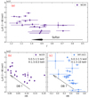 |
Fig. 4. Hardness intensity diagram of the 2021 outburst as monitored by NICER and Swift/XRT. The upper panel shows the results of the NICER spectral analysis, and the lower panels show the results based on HR. There is evidence that the source has entered the DB, thus the system appears to be close to or above the critical regime. |
3.3. Temporal properties – pulse profiles
To search for a periodic signal, we used the epoch-folding Z-search method (Buccheri et al. 1983) implemented through HENdrics command-line scripts and Stingray (Huppenkothen et al. 2019). For NuSTAR data, we searched for a periodic signal in the 3–40.0 keV range (35-960 PI channel). Our final estimate of the spin period and its uncertainties was based on the time of arrival (ToA) method (e.g., Tsygankov et al. 2020). We first used HENdrics to derive a most probable period, then we estimated ToAs of individual pulses for 16 intervals, and we finally used PINT3 (Luo et al. 2021). From the above we derived a period of 15.6395 ± 0.0004 s for the 2021 NuSTAR data. The reported period for the 2016 data was 15.6398 ± 0.0009 s and is consistent within the uncertainties with the newly derived period. For consistency, we implemented the ToA procedure to estimate a period for the 2016 Chandra data. Results of the ToA method are presented in Table 2. This yielded a period of 15.6396 ± 0.0014 s. All tests indicated that the period of the NS has remained unchanged within uncertainties for more than five years.
Spin periods SXP 15.6.
The strength of the periodic modulation is typically quantified through the root-mean-squared (rms) pulsed fraction (PF). This is given by
 (1)
(1)
where N is the number of phase bins, Rj is the background-subtracted count rate in the jth phase bin, and  is the average count rate in all bins (e.g., Wilson-Hodge et al. 2018). We used this definition to estimate the PFrms in different NuSTAR energy bands. We found no significant change in the PF within different energy bands up to 20 keV. However, above 20 keV, the PF increases and the pulsations become almost twice as strong at the highest energies. We also note that at above 40 keV, the contribution of background photons is ∼50% of the net counts. The increasing PF with energy is typical for accreting pulsars and is attributed to hard photons that are emitted from the sides of the accretion column. They are more beamed than soft photons (e.g., Lutovinov & Tsygankov 2009).
In Fig. 5 we present the folded pulse profiles for different energy bands covering the full NuSTAR energy range. We opted to also show the soft energy band (1.6–5.0 keV) in order to compare with NICER and Chandra pulse profiles. In Fig. A.1 we present the folded pulse profiles from all NICER observations for which a period could be estimated.
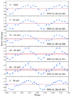 |
Fig. 5. Pulse profiles of SXP 15.6 from the NuSTAR observation. Different energy ranges are used to track the changes with energy. Shaded horizontal regions denote the limit of the statistical significant variability above the constant level hypothesis. |
3.4. Spin evolution
To investigate the spin evolution during the outburst, we implemented the same method on the NICER data between 0.5 and 8.0 keV. We first computed the most probable period by epoch folding, and then we refined the period and its uncertainty based on the ToA of individual pulses. Given the shape of the pulse profile, the template used for ToAs can drastically vary from one observation to the next. Thus, we used one universal template for all observations to characterise the off-phase of the pulse. The method was successful when two conditions occurred. Firstly, we need more than three NICER snapshots to be performed within one day, and secondly, the total number of counts must be high enough to obtain meaningful pulse profiles. For all other snapshot phases, it was challenging to connect the ToAs and even impossible at times due to multiple peaks in the periodogram with similar intensity. This problem is often encountered in slow pulsars that are observed with gaps (e.g., Zolotukhin et al. 2017; Vasilopoulos et al. 2018a).
The period evolution is shown in Fig. 6. The overall trend seems linear, although a large gap occurs in the data. Although due to the sampling variability due to orbital Doppler shifts is visible, the span of the NICER points with good timing solutions is ∼33 d and is comparable to the ∼36.4 d optical period. Thus the secular evolution between the first and last point alone should not be affected much by orbital effects. With this assumption, we found an average spin-up of Ṗ = (7.0 ± 2.5) × 10−10 s s−1 (or  Hz s−1). This value should be the approximate intrinsic spin-up due to accretion. Alternatively, the intrinsic spin up of the NS can be calculated (see Vasilopoulos et al. 2019, 2020, for method) due to the mass accretion rate as derived by the observed bolometric LX (see Fig. 3).
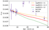 |
Fig. 6. Period evolution of SXP 15.6 within the 2021 outburst. The predicted spin-up rate based on the observed luminosity and three values of the magnetic field are plotted with dashed lines. |
Here are the basic steps for our calculation. We assumed mass transfer from a Keplerian disk, thus the induced torque due to accretion alone is  . The total torque can be expressed in the form of Ntot = n(ωfast)Nacc, where n(ωfast) is a dimensionless function that accounts for the coupling of the magnetic field lines to the accretion disk (for details, see Wang 1995; Parfrey et al. 2016). The spin-up rate of the NS is then given by
 (2)
(2)
where INS ≃ (1 − 1.7)×1045 g cm2 is the moment of inertia of the NS (e.g., Steiner et al. 2015).
To model the intrinsic spin evolution due to accretion, we just need to numerically solve Eq. (2) in time assuming a constant magnetic field strength. We used 1000 time steps in this span over the NICER monitoring. For each time step, the mass accretion was estimated by interpolating the observed flux in the 0.3–10 keV (see Fig. 2). Then we converted the flux into bolometric luminosity assuming the spectral parameters of the broadband spectra. Bolometric luminosity was then used as a proxy for mass accretion (i.e., LX = GṀM/R). For n(ωfast), we followed the Wang (1995) model (see their Eq. (19)). For all calculations we adopted standard NS parameters (i.e. 12 km radius, 1.4 M⊙ mass and INS = 1.3 × 1045 g cm2). We repeated this process for various magnetic field strengths, while the results are shown in Fig. 6. It is evident that the observed secular spin up is consistent with a magnetic field strength close to 3 × 10¹¹ G, while very low (< 1011 G) or high (> 1012 G) B values seem to be inconsistent with observations. Because the first and last pointing are separated by about one orbital period, we can neglect any orbital effects in this first-order approximation. However, we investigate any effects in the next section.
3.5. Orbital evolution
The observed spin evolution shows significant variation from the expected evolution caused by the intrinsic spin-up that is due to accretion. The remaining residuals may be due to orbital modulation. Keplerian orbits are described with five orbital elements: the orbital period (Porb), the orbital eccentricity (e), the argument of periastron of the stellar orbit (ω), the velocity semi-projected axis (a sin i in light seconds), and for the orbital phase, we finally used the time of a mean longitude of 90 deg (i.e., Tπ/2). The orbital modulation is often modelled with the intrinsic spin-up due to accretion, as described in the previous section (see Sect. 3.4), for Fermi/GBM pulsars (Sugizaki et al. 2017). However, most of the GBM monitored pulsars are Galactic sources that are monitored for extensive periods. To model our data set, the parameter space must be properly modelled in order to identify degeneracies between the model parameters. Thus, to fit the model to the data, we implemented a nested sampling algorithm for a Bayesian parameter estimation and estimated posterior distributions for the parameters of the standard accretion torque models and binary orbital parameters. In terms of statistical treatment, similar methods have been used to model radial velocity curves from binary systems (Fulton et al. 2018).
To derive the posterior probability distributions and the Bayesian evidence, we used the nested sampling MC algorithm MLFriends (Skilling et al. 2004; Buchner 2019) that employs the ULTRANEST4 package (Buchner 2021). An outline of this method with applications to accreting pulsars will be presented by Karaferias et al. (2022).
Because of the gaps in the NICER monitoring and the high background, good-timing data exist only for the first 20 days of the monitoring. In an effort to improve our data set, we also searched for pulsations in Swift/XRT data. However, because of the low statistics and small number of XRT snapshots within a day, typical period uncertainties were about 0.01–0.05 s (see Fig. 7). They therefore offer little information for our study. To constrain our model parameters, we fixed the orbital period to 36.411 days and limited the magnetic field strength (i.e., log(B[G]) ∈ [10, 13]). With these assumptions and for typical parameters of the NS (12 km and 1.4 M⊙), we estimated the posterior distribution for our other model parameters. These parameters are listed in Table 3, while in Fig. A.2 we show the corner plot of posterior distributions for our solution. In Fig. 7 we show a sample of 100 random orbital models from the posterior distribution together with the most probable model.
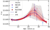 |
Fig. 7. Modelling of the spin period evolution of SXP 15.6 based on orbital modulation and intrinsic spin-up. The most probable solution is shown as the dashed line, and the dotted black line shows the Doppler shifts due to orbital modulation alone, without the spin-up due to accretion. A family of orbits drawn from the sample of the posterior distribution of parameters from the Bayesian modelling is shown as red lines. The shaded region is the 99% quantile of the models. Although Swift/XRT data present hits of periodic modulation, the uncertainties are quite high and cannot constrain our model. For visualisation purposes, we plot one of these XRT measurements. |
Orbital parameters of the binary SXP 15.6.
4. Discussion
The latest outburst of SXP 15.6 started in late November 2021, while the system remained in a bright state until early 2022. The bolometric luminosity during the event reached 7 × 1037 erg s−1, which presents the brightest stage ever observed for the system. This luminosity translates into ∼30% of the Eddington limit for a typical NS (i.e., 12 km and 1.4 M⊙).
The combined Swift/XRT and NICER light curve of the 2021 outburst reveals a complex structure with two peaks separated by the orbital period. The increased flux at later epochs indicates a third peak, but not enough monitoring data were collected to further explore this behaviour. The general structure of the event matches the behaviour seen in 2016 very well (see Fig. 3), with minor differences in the relative intensity of the three peaks. The mismatch of the X-ray and optical period could be attributed to a precessing decretion disk around the Be star (for an observational example and a theoretical application, see Treiber et al. 2021; Martin & Franchini 2021). This precession can cause an evolving period between outbursts if the disk is moving retrograde to the NS orbit. Nevertheless, the self-similarity of the 2016 and 2021 outbursts with three peaks is quite intriguing and reveals that the Be disk and the NS geometrical configuration behave in a repetitive manner.
The NS spin evolution shows evidence of orbital and intrinsic spin-up due to accretion. Because the first and last day of the NICER observations (MJD 59535-75 interval) consisted of a large number of snapshots, we were able to constrain the intrinsic spin-up and found a value of  Hz s−1. To improve this estimate, we simultaneously modelled the orbital modulation and intrinsic spin-up with a Bayesian approach. We found that the spin-up is consistent with an NS pulsar with a magnetic field strength of 5 × 10¹¹ G with an uncertainty of a factor of ∼3. Moreover, the orbit has a moderate eccentricity with a value of ∼0.29, while values up to 0.6 cannot be statistically excluded. Interestingly, the corner plot in Fig. A.2 shows that lower magnetic fields are apparently favoured by more eccentric orbits, and the uncertainties in some parameters are still high. From the orbital parameters (i.e., ω and Tπ/2) we can also estimate the epoch of periastron Tper, which is found to be MJD 59531 ± 4. The value of Tper seems to match or lead by a few days the X-ray maxima observed in the X-ray light curve (see Fig. 3). Figure 7 interestingly shows that quite a few orbits with higher eccentricity are still statistically acceptable and cannot be excluded without better data. Future independent measurements that could constrain the orbital parameters would help us revisit the system and tighten the constraints on the magnetic field strength.
The value of the magnetic field that we estimate can be compared with the estimates of Coe et al. (2022), who found a value of 3.7 × 10¹² G, assuming the source is in spin equilibrium. For an NS pulsar to rotate near spin-equilibrium, constant mass accretion is assumed and the disk inner radius is required to rotate with about the same angular velocity as the NS. However, there are a few caveats in these assumptions. Because BeXRBs are extremely variable systems, the assumption of steady accretion does not hold, and for systems rotating near equilibrium, torque transfer is a non-linear problem. Moreover, rotation near equilibrium does not mean that the spin-up rate is zero. Under the assumption of steady accretion, even some of the systems with the highest spin-up rate can be argued to be near equilibrium (Pan et al. 2022). In addition, finding the secular spin evolution to be very small does not necessarily mean that the NS is in equilibrium. The spin evolution is a dynamical problem in which the accretion duty cycle plays an equally important role in determining any secular spin change between two epochs. Estimates of the magnetic field assuming spin-equilibrium are therefore subject to large systematic uncertainties and should be considered much less accurate than our estimates from torque modelling.
The broadband spectra from the combined NuSTAR and NICER observations lack any significant line features that could be associated with emission from hot plasma (e.g., an Fe Kα line) or a CRSF. The high-energy part of the spectrum is well explained by a power law with a cut-off in agreement with other BeXRBs. However, the soft part of the spectrum requires additional components in order to be explained. We tested whether the addition of a thermal component or a partial absorber could improve the quality of the fit. Either or both of these components would result in an acceptable fit.
The thermal component is particularly interesting because it can be interpreted as the inner region of an accretion disk. An analytical form for the magnetospheric radius can be expressed in the following form (Frank et al. 2002; Campana et al. 2018):
 (3)
(3)
where M is the NS mass, μ = BR3/2 is the magnetic dipole moment, with R the NS radius and B the NS magnetic field strength at the magnetic poles. For typical parameters of the NS (12 km and 1.4 M⊙) and for the observed mass-accretion rate and assuming a polar magnetic field strength of 5 × 10¹¹ G, the disk radius should be about 600 km. However, our best-fit spectral model yields a much smaller inner disk radius (i.e., ∼15 − 20 km, see Table 1), which is comparable to the NS radius. This radius would translate into a B value of 109 G, which is unrealistically small for a BeXRB pulsar. This value is also at odds with the results of the torque modelling because Fig. 7 shows that a magnetic field lower than 1011 G would not be able to explain the spin evolution over the 30-day period, unless a quite eccentric orbit is assumed. Because the disk could be seen edge on, another way to estimate its size is from its temperature. By adopting the mass-accretion rate from the pulsed continuum and for a temperature of 0.4 keV (from the fit), the inner radius of a standard disk would be about 60–70 km, depending on the spectral hardening parameter (see Kubota et al. 1998; Zimmerman et al. 2005). This is still significantly smaller than the size estimated from torque modelling, which predicts a disk size of about 600 km for a magnetic field of 5 × 10¹¹ G and Ṁ ∼ 2.5 × 10¹⁷ g s−1. For these parameters, the disk temperature should be ∼70 eV. As seen in the last column of Table 1, a model with a disk with a temperature fixed at 70 eV can sufficiently explain the observed spectra. The disk size for this temperature is about 200–900 km.
With respect to the partial coverage model, the rationale behind this model is that the line of sight between the observer and the source is not a line in a mathematical sense. Because of the extent of the emitting region, the geometrical problem is better described as a superposition of multiple line of sights. The absorber present in the vicinity of the source can be imagined as a collection of dense clouds that lie inside the magnetosphere or engulf the binary itself. Partial covering manifests itself as broad humps or bumps below 10 keV depending on the column density of the partial absorber. For example for the Galactic pulsars GX 304-1 and Her X-1, the partial absorber has typical values of NH ∼ 10 − 70 × 1022 cm−1 and a covering fraction of 30–40% depending on the selection of the continuum model (e.g., Endo et al. 2000; Asami et al. 2014; Jaisawal et al. 2016). These values are quite similar to the values we find in SXP 15.6 and other BeXRB systems in the MCs (e.g., Vasilopoulos et al. 2018b).
This discussion demonstrates the complexity of the soft excess, which in our case cannot be modelled without overfitting the data. Thus we caution about the spectral parameters for the soft excess. For these empirical models, a physical interpretation is difficult because an acceptable goodness of fit and almost flat spectral residuals can be obtained for a wide range of parameters.
We can use the results of the broadband spectroscopy to convert observed fluxes in the 0.3–10.0 keV band into bolometric luminosities. The bolometric correction is ∼3.5–4, where its uncertainty is due to the model selection because partial covering models generally give higher unabsorbed flux. This is slightly higher than what is observed in accreting pulsars, since the study of nine frequently observed Galactic systems has shown that 37–62% of the energy is released in the 0.5–10.0 keV band, when the total Luminosity is below the Eddington limit (Anastasopoulou et al. 2022). The value we find is consistent (within 2σ) with the expected value in the observed luminosity range as determined by Anastasopoulou et al. (2022). The bolometric correction is important if we would like to track transitions in the spectral properties associated with changes in the accretion column (Becker et al. 2012). Following Reig & Nespoli (2013), we can argue that the spectral behaviour during the 2021 monitoring is consistent with the super-critical regime. This means that we are above the critical luminosity where the accretion column has started to form (see also Postnov et al. 2015). Following Becker et al. (2012) this luminosity is given by
 (4)
(4)
which holds for typical parameters (see Eq. (32) of Becker et al. 2012, for more details). From the colour intensity diagram (see Fig. 4) we can set an upper limit to the critical transition and thus the magnetic field of the NS. For Lcrit of ∼1037 erg s−1 we found an upper limit for the magnetic field of about 0.7 × 10¹² G. This quantitative estimate seems to agree with the lack of any evident CRSF in the broadband spectrum. Such a feature would appear at energies (ECRSF) and be related to the magnetic field through the following relation:
 (5)
(5)
where z ∼ 0.3 is the gravitational redshift from the NS, which is related to the NS compactness (e.g., Riley et al. 2019). The upper limit for the critical luminosity would thus translate into an upper limit for the ECRSF of ∼6 keV. Because the spectrum at lower energies is complex and there is soft excess, it is thus not surprising that we did not detect any CRSF in the spectrum. This is also consistent with the fact that no accreting pulsar has a detected electron CRSF below 8 keV, and claims of such detections in some systems still wait to be confirmed (Staubert et al. 2019).
The pulse shape of the pulse profile is single peaked (Figs. 5 and A.1). At higher energies (> 40 keV), the pulse profile is sharper, with a triangular shape, while it appears to be broader in the soft band, with weak evidence of a secondary peak. We note the similarity of the pulse profile in the soft NuSTAR band (see Fig. 5) to the profiles obtained from the NICER monitoring (see Fig. A.1). A single-peaked pulse profile at what otherwise appears to be close to or above the critical limit for the super-critical regime is quite unusual because complex profiles are the norm for these bright BeXRBs (e.g., Epili et al. 2017; Koliopanos & Vasilopoulos 2018). Further investigation of the pulse profiles with physical models (e.g., Cappallo et al. 2017; Mushtukov et al. 2018) could provide further information of this somewhat puzzling feature.
5. Conclusions
We have analysed broadband spectra from the 2021 outburst of SXP 15.6. We did not identify any CRSF that could provide a direct measurement of the NS magnetic field. Nevertheless, the lack of such a feature does not exclude its presence because a CRSF could also be quite weak or depend on the pulse phase (e.g., Tiengo et al. 2013). In the broadband spectra, we found evidence of a soft spectral component that could be associated with an accretion disk, but its parameters are poorly constrained. An alternative explanation is that the soft excess is a result of partial absorption, and we do not favour one model over the other. The evolution of the spectral properties during the 2021 outburst is consistent with an accretion column above the NS and with the system accreting close to or above the critical limit. Finally, we did not measure any secular evolution of the spin period of the pulsar between 2016 Chandra and 2021 NuSTAR observations, which is consistent with the findings of Coe et al. (2022). Nevertheless, there is evident modulation in the NICER monitoring data that is consistent with orbital motion of the binary. Modelling of the orbital motion and intrinsic spin-up during the outburst enabled us to constrain the magnetic field strength and the orbital parameters of the system. All the derived quantitative and qualitative results consistently provide indirect constraints on the NS magnetic field strength. Because a cyclotron line is lacking, the most reliable measurement comes from the intrinsic spin up, based on which we find a value of 5 × 10¹¹ G with an uncertainty of about a factor of ∼3.
I.e. LX = GṀM/R ≈ 0.2 Ṁc2(M/1.4 M⊙)(R/10 km)−1.
Acknowledgments
The authors would like to thank the anonymous referee for the constructive report that helped to greatly improve the manuscript. GV would like to thank P.S. Ray for his comments, suggestions and advice on using PINT. This work was supported by NASA through the NICER mission and the Astrophysics Explorers Program. Facilities: NICER, NuSTAR. We acknowledge the use of public data from the Swift data archive.
References
- Anastasopoulou, K., Zezas, A., Steiner, J. F., & Reig, P. 2022, MNRAS, 513, 1400 [NASA ADS] [CrossRef] [Google Scholar]
- Arnaud, K. A. 1996, in Astronomical Data Analysis Software and Systems V, eds. G. H. Jacoby, & J. Barnes, ASP Conf. Ser., 101, 17 [NASA ADS] [Google Scholar]
- Asami, F., Enoto, T., Iwakiri, W., et al. 2014, PASJ, 66, 44 [NASA ADS] [CrossRef] [Google Scholar]
- Becker, P. A., & Wolff, M. T. 2007, ApJ, 654, 435 [NASA ADS] [CrossRef] [Google Scholar]
- Becker, P. A., Klochkov, D., Schönherr, G., et al. 2012, A&A, 544, A123 [NASA ADS] [CrossRef] [EDP Sciences] [Google Scholar]
- Buccheri, R., Bennett, K., Bignami, G. F., et al. 1983, A&A, 128, 245 [NASA ADS] [Google Scholar]
- Buchner, J. 2019, PASP, 131, 108005 [Google Scholar]
- Buchner, J. 2021, J. Open Source Softw., 6, 3001 [CrossRef] [Google Scholar]
- Burrows, D. N., Hill, J. E., Nousek, J. A., et al. 2005, Space Sci. Rev., 120, 165 [Google Scholar]
- Campana, S., Stella, L., Mereghetti, S., & de Martino, D. 2018, A&A, 610, A46 [NASA ADS] [CrossRef] [EDP Sciences] [Google Scholar]
- Cappallo, R., Laycock, S. G. T., & Christodoulou, D. M. 2017, PASP, 129, 124201 [NASA ADS] [CrossRef] [Google Scholar]
- Cash, W. 1979, ApJ, 228, 939 [Google Scholar]
- Coe, M. J., Evans, P. A., Kennea, J. A., et al. 2021, The ATel, 15054, 1 [NASA ADS] [Google Scholar]
- Coe, M. J., Monageng, I. M., Kennea, J. A., et al. 2022, MNRAS, 513, 5567 [NASA ADS] [Google Scholar]
- Dickey, J. M., & Lockman, F. J. 1990, ARA&A, 28, 215 [Google Scholar]
- Endo, T., Nagase, F., & Mihara, T. 2000, PASJ, 52, 223 [NASA ADS] [Google Scholar]
- Epili, P., Naik, S., Jaisawal, G. K., & Gupta, S. 2017, MNRAS, 472, 3455 [CrossRef] [Google Scholar]
- Evans, P. A., Beardmore, A. P., Page, K. L., et al. 2007, A&A, 469, 379 [NASA ADS] [CrossRef] [EDP Sciences] [Google Scholar]
- Evans, P. A., Beardmore, A. P., Page, K. L., et al. 2009, MNRAS, 397, 1177 [Google Scholar]
- Frank, J., King, A., & Raine, D. J. 2002, Accretion Power in Astrophysics, 3rd edn. (Cambridge: Cambridge University Press) [Google Scholar]
- Fruscione, A., McDowell, J. C., Allen, G. E., et al. 2006, Proc. SPIE, 6270, 62701V [Google Scholar]
- Fulton, B. J., Petigura, E. A., Blunt, S., & Sinukoff, E. 2018, PASP, 130, 044504 [Google Scholar]
- Gehrels, N., Chincarini, G., Giommi, P., et al. 2004, ApJ, 611, 1005 [Google Scholar]
- Gendreau, K. C., Arzoumanian, Z., & Okajima, T. 2012, in The Neutron star Interior Composition ExploreR (NICER): an Explorer Mission of Opportunity for Soft x-ray Timing Spectroscopy, SPIE Conf. Ser., 8443, 844313 [NASA ADS] [Google Scholar]
- Gendreau, K. C., Arzoumanian, Z., Adkins, P. W., et al. 2016, in The Neutron star Interior Composition Explorer (NICER): Design and Development, SPIE Conf. Ser., 9905, 99051H [NASA ADS] [Google Scholar]
- Graczyk, D., Pietrzyński, G., Thompson, I. B., et al. 2014, ApJ, 780, 59 [Google Scholar]
- Haberl, F., & Sturm, R. 2016, A&A, 586, A81 [NASA ADS] [CrossRef] [EDP Sciences] [Google Scholar]
- Harrison, F. A., Craig, W. W., Christensen, F. E., et al. 2013, ApJ, 770, 103 [Google Scholar]
- Hickox, R. C., Narayan, R., & Kallman, T. R. 2004, ApJ, 614, 881 [NASA ADS] [CrossRef] [Google Scholar]
- Huppenkothen, D., Bachetti, M., Stevens, A. L., et al. 2019, ApJ, 881, 39 [Google Scholar]
- Jaisawal, G. K., & Naik, S. 2016, MNRAS, 461, L97 [NASA ADS] [CrossRef] [Google Scholar]
- Jaisawal, G. K., Naik, S., & Chenevez, J. 2018, MNRAS, 474, 4432 [NASA ADS] [CrossRef] [Google Scholar]
- Jaisawal, G. K., Naik, S., & Epili, P. 2016, MNRAS, 457, 2749 [NASA ADS] [CrossRef] [Google Scholar]
- Karaferias, A. S., Vasilopoulos, G., Petropoulou, M., et al. 2022, MNRAS, submitted [Google Scholar]
- Kennea, J. A., Coe, M. J., Evans, P. A., et al. 2016, The ATel, 9362, 1 [NASA ADS] [Google Scholar]
- Kennea, J. A., Coe, M. J., Evans, P. A., Waters, J., & Jasko, R. E. 2018, ApJ, 868, 47 [NASA ADS] [CrossRef] [Google Scholar]
- Koliopanos, F., & Vasilopoulos, G. 2018, A&A, 614, A23 [NASA ADS] [EDP Sciences] [Google Scholar]
- Kubota, A., Tanaka, Y., Makishima, K., et al. 1998, PASJ, 50, 667 [NASA ADS] [CrossRef] [Google Scholar]
- Luo, J., Ransom, S., Demorest, P., et al. 2021, ApJ, 911, 45 [NASA ADS] [CrossRef] [Google Scholar]
- Lutovinov, A. A., & Tsygankov, S. S. 2009, Astron. Lett., 35, 433 [NASA ADS] [CrossRef] [Google Scholar]
- Maitra, C., Paul, B., Haberl, F., & Vasilopoulos, G. 2018, MNRAS, 480, L136 [NASA ADS] [CrossRef] [Google Scholar]
- Martin, R. G., & Franchini, A. 2021, ApJ, 922, L37 [NASA ADS] [CrossRef] [Google Scholar]
- Martin, R. G., Nixon, C., Armitage, P. J., Lubow, S. H., & Price, D. J. 2014, ApJ, 790, L34 [Google Scholar]
- McBride, V. A., González-Galán, A., Bird, A. J., et al. 2017, MNRAS, 467, 1526 [NASA ADS] [CrossRef] [Google Scholar]
- Müller, S., Ferrigno, C., Kühnel, M., et al. 2013, A&A, 551, A6 [NASA ADS] [CrossRef] [EDP Sciences] [Google Scholar]
- Mushtukov, A. A., Verhagen, P. A., Tsygankov, S. S., et al. 2018, MNRAS, 474, 5425 [NASA ADS] [CrossRef] [Google Scholar]
- Okazaki, A. T., Hayasaki, K., & Moritani, Y. 2013, PASJ, 65, 41 [NASA ADS] [Google Scholar]
- Pan, Y. Y., Li, Z. S., Zhang, C. M., & Zhong, J. X. 2022, MNRAS, 513, 6219 [NASA ADS] [CrossRef] [Google Scholar]
- Parfrey, K., Spitkovsky, A., & Beloborodov, A. M. 2016, ApJ, 822, 33 [NASA ADS] [CrossRef] [Google Scholar]
- Postnov, K. A., Gornostaev, M. I., Klochkov, D., et al. 2015, MNRAS, 452, 1601 [Google Scholar]
- Prigozhin, G., Gendreau, K., Foster, R., et al. 2012, in Characterization of the Silicon Drift Detector for NICER instrument, SPIE Conf. Ser., 8453, 845318 [NASA ADS] [Google Scholar]
- Reig, P. 2011, Ap&SS, 332, 1 [Google Scholar]
- Reig, P., & Nespoli, E. 2013, A&A, 551, A1 [NASA ADS] [CrossRef] [EDP Sciences] [Google Scholar]
- Remillard, R. A., Loewenstein, M., Steiner, J. F., et al. 2022, AJ, 163, 130 [NASA ADS] [CrossRef] [Google Scholar]
- Riley, T. E., Watts, A. L., Bogdanov, S., et al. 2019, ApJ, 887, L21 [Google Scholar]
- Russell, S. C., & Dopita, M. A. 1992, ApJ, 384, 508 [NASA ADS] [CrossRef] [Google Scholar]
- Skilling, J. 2004, in American Institute of Physics Conference Series, eds. R. Fischer, R. Preuss, & U. V. Toussaint, 735, 395 [NASA ADS] [Google Scholar]
- Staubert, R., Trümper, J., Kendziorra, E., et al. 2019, A&A, 622, A61 [NASA ADS] [CrossRef] [EDP Sciences] [Google Scholar]
- Steiner, A. W., Gandolfi, S., Fattoyev, F. J., & Newton, W. G. 2015, Phys. Rev. C, 91, 015804 [NASA ADS] [CrossRef] [Google Scholar]
- Sturm, R., Haberl, F., Vasilopoulos, G., et al. 2014, MNRAS, 444, 3571 [NASA ADS] [CrossRef] [Google Scholar]
- Sugizaki, M., Mihara, T., Nakajima, M., & Makishima, K. 2017, PASJ, 69, 100 [NASA ADS] [CrossRef] [Google Scholar]
- Tiengo, A., Esposito, P., Mereghetti, S., et al. 2013, Nature, 500, 312 [CrossRef] [Google Scholar]
- Treiber, H., Vasilopoulos, G., Bailyn, C. D., et al. 2021, MNRAS, 503, 6187 [CrossRef] [Google Scholar]
- Tsygankov, S. S., Doroshenko, V., Mushtukov, A. A., et al. 2020, A&A, 637, A33 [NASA ADS] [CrossRef] [EDP Sciences] [Google Scholar]
- Vasilopoulos, G., Maggi, P., Haberl, F., et al. 2013, A&A, 558, A74 [NASA ADS] [CrossRef] [EDP Sciences] [Google Scholar]
- Vasilopoulos, G., Haberl, F., Delvaux, C., Sturm, R., & Udalski, A. 2016, MNRAS, 461, 1875 [NASA ADS] [CrossRef] [Google Scholar]
- Vasilopoulos, G., Haberl, F., & Maggi, P. 2017a, MNRAS, 470, 1971 [NASA ADS] [CrossRef] [Google Scholar]
- Vasilopoulos, G., Zezas, A., Antoniou, V., & Haberl, F. 2017b, MNRAS, 470, 4354 [NASA ADS] [CrossRef] [Google Scholar]
- Vasilopoulos, G., Haberl, F., Carpano, S., & Maitra, C. 2018a, A&A, 620, L12 [NASA ADS] [EDP Sciences] [Google Scholar]
- Vasilopoulos, G., Maitra, C., Haberl, F., Hatzidimitriou, D., & Petropoulou, M. 2018b, MNRAS, 475, 220 [Google Scholar]
- Vasilopoulos, G., Petropoulou, M., Koliopanos, F., et al. 2019, MNRAS, 488, 5225 [Google Scholar]
- Vasilopoulos, G., Ray, P. S., Gendreau, K. C., et al. 2020, MNRAS, 494, 5350 [NASA ADS] [CrossRef] [Google Scholar]
- Verner, D. A., Ferland, G. J., Korista, K. T., & Yakovlev, D. G. 1996, ApJ, 465, 487 [Google Scholar]
- Wang, Y.-M. 1995, ApJ, 449, L153 [NASA ADS] [Google Scholar]
- Wilms, J., Allen, A., & McCray, R. 2000, ApJ, 542, 914 [Google Scholar]
- Wilson-Hodge, C. A., Malacaria, C., Jenke, P. A., et al. 2018, ApJ, 863, 9 [Google Scholar]
- Zimmerman, E. R., Narayan, R., McClintock, J. E., & Miller, J. M. 2005, ApJ, 618, 832 [NASA ADS] [CrossRef] [Google Scholar]
- Zolotukhin, I. Y., Bachetti, M., Sartore, N., Chilingarian, I. V., & Webb, N. A. 2017, ApJ, 839, 125 [NASA ADS] [CrossRef] [Google Scholar]
Appendix A: Additional figures and tables
 |
Fig. A.1. Pulse profiles (0.5–8.0 keV) of all NICER observations where significant pulsations were detectable. The labels within each panel denote the last three digits of the NICER obsid number, i.e. 4202430XXX. All profiles are normalised to the average intensity, and the minimum is shifted to zero phase. Shaded horizontal regions denote the limit of the statistically significant variability above the constant level hypothesis. For comparison, the 2016 pulse profile as measured by Chandra is plotted with a dotted grey line in each panel. |
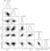 |
Fig. A.2. Corner plot for SXP 15.6 using the model described in the text. We plot the logarithm of the polar magnetic field strength B in G, the eccentricity (e), the longitude of periastron in degrees (ω), the projected semi-major axis in light seconds (a sin i), the time of a mean longitude of 90 degrees Tπ/2 and the pulsar frequency F0 in mHz. The reference epoch for F0 is the start of the NICER monitoring, i.e. MJD 59538.5. |
Power-law fit to NICER data.
All Tables
All Figures
|
Fig. 1. Broadband spectrum of SXP 15.6. NuSTAR spectra are shown in black, and two NICER snapshots are shown in red and cyan. The upper panel presents the best-fit model composed of an absorbed cut-off power law and a soft thermal component. The ratio plots show the comparison of the tested models and the data: (b) Absorbed cut-off power law, (c) absorbed cut-off power law plus disk blackbody, and (d) cut-off power law with partial coverage. The model parameters are listed in Table 1. |
| In the text | |
|
Fig. 2. Spectral results of NICER monitoring data obtained during the 2021 outburst of SXP 15.6. The bottom panel shows the unabsorbed flux computed in the 0.3–10.0 keV band. The red shaded region indicates the epoch of the NuSTAR ToO. No strong evidence for a change in the column density of the absorbing material (top panel) is seen, but we found evidence of spectral evolution at higher fluxes with the spectral shape (characterised by Γ, middle panel) becoming softer when brighter above 2× 10⁻¹¹ erg cm−2 s−1 (0.3–10.0 keV). |
| In the text | |
|
Fig. 3. X-ray light curves of the 2016 and 2021 outbursts. Luminosities are absorption corrected (0.3–80.0 keV) and computed for the SMC distance. Archival data from 2016 (first point at MJD 57547) are shifted in time to match the 2021 luminosity peaks. Vertical green lines mark the 36.411 d optical period phased on the first X-ray maximum. For comparison we also show the shifted epoch of the Chandra ToO that falls around the same orbital phase as the NuSTAR ToO. |
| In the text | |
|
Fig. 4. Hardness intensity diagram of the 2021 outburst as monitored by NICER and Swift/XRT. The upper panel shows the results of the NICER spectral analysis, and the lower panels show the results based on HR. There is evidence that the source has entered the DB, thus the system appears to be close to or above the critical regime. |
| In the text | |
|
Fig. 5. Pulse profiles of SXP 15.6 from the NuSTAR observation. Different energy ranges are used to track the changes with energy. Shaded horizontal regions denote the limit of the statistical significant variability above the constant level hypothesis. |
| In the text | |
|
Fig. 6. Period evolution of SXP 15.6 within the 2021 outburst. The predicted spin-up rate based on the observed luminosity and three values of the magnetic field are plotted with dashed lines. |
| In the text | |
|
Fig. 7. Modelling of the spin period evolution of SXP 15.6 based on orbital modulation and intrinsic spin-up. The most probable solution is shown as the dashed line, and the dotted black line shows the Doppler shifts due to orbital modulation alone, without the spin-up due to accretion. A family of orbits drawn from the sample of the posterior distribution of parameters from the Bayesian modelling is shown as red lines. The shaded region is the 99% quantile of the models. Although Swift/XRT data present hits of periodic modulation, the uncertainties are quite high and cannot constrain our model. For visualisation purposes, we plot one of these XRT measurements. |
| In the text | |
|
Fig. A.1. Pulse profiles (0.5–8.0 keV) of all NICER observations where significant pulsations were detectable. The labels within each panel denote the last three digits of the NICER obsid number, i.e. 4202430XXX. All profiles are normalised to the average intensity, and the minimum is shifted to zero phase. Shaded horizontal regions denote the limit of the statistically significant variability above the constant level hypothesis. For comparison, the 2016 pulse profile as measured by Chandra is plotted with a dotted grey line in each panel. |
| In the text | |
|
Fig. A.2. Corner plot for SXP 15.6 using the model described in the text. We plot the logarithm of the polar magnetic field strength B in G, the eccentricity (e), the longitude of periastron in degrees (ω), the projected semi-major axis in light seconds (a sin i), the time of a mean longitude of 90 degrees Tπ/2 and the pulsar frequency F0 in mHz. The reference epoch for F0 is the start of the NICER monitoring, i.e. MJD 59538.5. |
| In the text | |
Current usage metrics show cumulative count of Article Views (full-text article views including HTML views, PDF and ePub downloads, according to the available data) and Abstracts Views on Vision4Press platform.
Data correspond to usage on the plateform after 2015. The current usage metrics is available 48-96 hours after online publication and is updated daily on week days.
Initial download of the metrics may take a while.