| Issue |
A&A
Volume 697, May 2025
|
|
|---|---|---|
| Article Number | A207 | |
| Number of page(s) | 15 | |
| Section | Extragalactic astronomy | |
| DOI | https://doi.org/10.1051/0004-6361/202452659 | |
| Published online | 19 May 2025 | |
Classifying merger stages with adaptive deep learning and cosmological hydrodynamical simulations
1
Kapteyn Astronomical Institute, University of Groningen, Postbus 800, 9700 AV Groningen, The Netherlands
2
SRON Netherlands Institute for Space Research, Landleven 12, 9747 AD Groningen, The Netherlands
3
National Centre for Nuclear Research, Pasteura 7, 02-093 Warszawa, Poland
4
Instituto de Radioastronomía y Astrofísica, Universidad Nacional Autónoma de México, Apdo. Postal 72-3, 58089 Morelia, Mexico
5
Dunlap Institute for Astronomy and Astrophysics, University of Toronto, 50 St. George Street, Toronto, ON M5S 3H4, Canada
⋆ Corresponding author: This email address is being protected from spambots. You need JavaScript enabled to view it.
Received:
18
October
2024
Accepted:
9
March
2025
Abstract
Aims. Hierarchical merging of galaxies plays an important role in galaxy formation and evolution. Mergers could trigger key evolutionary phases such as starburst activities and active accretion periods onto supermassive black holes at the centres of galaxies. We aim to detect mergers and merger stages (pre- and post-mergers) across cosmic history. Our main goal is to test whether it is more beneficial to detect mergers and their merger stages simultaneously or hierarchically. In addition, we wish to test the impact of merger time relative to the coalescence of merging galaxies.
Methods. First, we generated realistic mock James Webb Space Telescope (JWST) images of simulated galaxies selected from the IllustrisTNG cosmological hydrodynamical simulations. The advantage of using simulations is that we have information on both whether a galaxy is a merger and its exact merger stage (i.e. when in the past or in the future the galaxy has experienced or will experience a merging event). Then, we trained deep-learning (DL) models for galaxy morphology classifications in the Zoobot Python package to classify galaxies into non-merging galaxies, merging galaxies and their merger stages. We used two different set-ups, a two-stage set-up versus a one-stage set-up. In the former set-up, we first classified galaxies into mergers and non-mergers, and we then classified the mergers into pre-mergers and post-mergers. In the latter set-up, non-mergers, pre-mergers and post-mergers were classified simultaneously.
Results. We found that the one-stage classification set-up moderately outperforms the two-stage set-up. It offers a better overall accuracy and generally a better precision, particularly for the non-merger class. Out of the three classes, pre-mergers can be classified with the highest precision (∼65% versus ∼33% from a random classifier) in both set-ups, possibly because the merging features are generally more easily recognised, and because there are merging companions. More confusion is found between post-mergers and non-mergers than between these two classes and pre-mergers. The image signal-to-noise ratio (S/N) also affects the performance of the DL classifiers, but not by much after a certain threshold is crossed (S/N ∼ 20 in a 0.2″aperture). In terms of the merger timescale, both precision and recall of the classifiers strongly depend on merger time. Both set-ups find it more difficult to identify true mergers that are observed at stages that are farther from coalescence either in the past or in the future. For pre-mergers, we recommend selecting mergers that will merge in the next 0.4 Gyr to achieve a good balance between precision and recall.
Key words: techniques: image processing / galaxies: active / galaxies: evolution / galaxies: interactions
© The Authors 2025
 Open Access article, published by EDP Sciences, under the terms of the Creative Commons Attribution License (https://creativecommons.org/licenses/by/4.0), which permits unrestricted use, distribution, and reproduction in any medium, provided the original work is properly cited.
This article is published in open access under the Subscribe to Open model. This email address is being protected from spambots. You need JavaScript enabled to view it. to support open access publication.
1. Introduction
In the widely accepted hierarchical structure formation paradigm (White & Frenk 1991; Cole et al. 2000), galaxies collide and merge with each other throughout cosmic time. This fundamentally affects the way in which galaxies form and evolve. This process can be and still is seen today in the very local Universe. For example, our own Milky Way has had several merging events in the past, as revealed via stellar streams, and it heads towards a collision course with the neighbouring Andromeda galaxy in the future (review by Helmi 2020, and references therein). Over the past several decades, there have been numerous studies on measuring the merger history of galaxies all the way from the present-day Universe to the epoch of reionisation (Conselice et al. 2003, 2022; Lotz et al. 2011; Duncan et al. 2019; Ferreira et al. 2020), as well as on deciphering the role of merging in galaxy mass assembly, morphological transformation, triggering of accretion episodes onto supermassive black holes (SMBH), and star-formation activity (Ellison et al. 2008, 2019; Patton et al. 2011; Satyapal et al. 2014; Goulding et al. 2018; Pearson et al. 2019a, 2022; Gao et al. 2020; Villforth 2023; La Marca et al. 2024).
However, despite the huge progress that has already been made, we still do not understand the relative importance of mergers and secular evolution, in particular, in the more distant Universe or if there are definitive links (and how they evolve) between mergers and key galaxy evolution phases such as starbursts and active galactic nuclei (AGN). One of the main challenges faced by studies involving galaxy mergers is the merger detection. Various methods have been used in the past to identify merging galaxies, for instance, counting galaxy pairs in photometric or spectroscopic data (Lambas et al. 2012; Knapen et al. 2015; Duan et al. 2025) and detecting morphologically disturbed galaxies using non-parametric statistics, such as the concentration-asymmetry-smoothness (CAS) parameters, M20 (the second-order moment of the brightest 20% of the light), and the Gini coefficient (Conselice et al. 2000; Conselice 2003; Lotz et al. 2004, 2008), or visual inspection, such as expert classification labels (Kartaltepe et al. 2015) or volunteer labels from the Galaxy Zoo (GZ) citizen science project (Lintott et al. 2008, 2011; Darg et al. 2010). Different methods have different advantages and disadvantages that were extensively discussed in many previous works (Huertas-Company et al. 2015; Snyder et al. 2019; Blumenthal et al. 2020; Margalef-Bentabol et al. 2024). According to hydrodynamical simulations, starburst, quenching of star formation, and accretion onto SMBHs take place at different stages (Hopkins et al. 2008; Blecha et al. 2018; Rodríguez Montero et al. 2019; Liao et al. 2023; Quai et al. 2023; Byrne-Mamahit et al. 2024). Therefore, beyond a binary classification of merging and non-merging galaxies, it is also important to place merging galaxies on their merging sequences, which typically last about some billion years. However, so far, our knowledge of merger stages beyond a basic pre-merger and post-merger separation (i.e. merging galaxies caught before and after coalescence) is extremely limited.
With the advent of deep-learning (DL; Goodfellow et al. 2016) techniques that excel in computer vision tasks and increasingly more realistic cosmological hydro-dynamical simulations (Vogelsberger et al. 2014; Dubois et al. 2014; Schaye et al. 2015; Nelson et al. 2019), some of the fundamental limitations of previous studies can be better addressed or even overcome. Large samples of realistic merging galaxies at different stages along their merging sequences (via information on galaxy merger tree histories) are now available from cosmological simulations, and they can be used to train or test merger detection algorithms with reliable truth labels. This means that we are no longer limited to classification labels derived from visual inspection, which is subjective, (often) unreliable, incomplete, and time-consuming to obtain. For the first time, we can quantitatively assess the levels of completeness and reliability for any merger detection algorithm, which is essential for statistical studies such as measurements of galaxy merger fractions and merger rates. At the same time, there has been an explosion over the past decade in applying DL techniques, in particular, convolutional neural networks (CNNs; Lecun et al. 1998; Krizhevsky et al. 2012), to astronomical questions (e.g. galaxy morphological classifications and detections of strongly lensed galaxies) and many of them have shown great success (Dieleman et al. 2015; Huertas-Company et al. 2015; Petrillo et al. 2017; Schaefer et al. 2018; Li et al. 2020). For a review, we refer to Huertas-Company & Lanusse (2023).
The first example of an application of DL CNNs for the detection of galaxy mergers was presented in Ackermann et al. (2018). The CNN was trained on the imagenet dataset (Deng et al. 2009) and visual classification labels from the GZ. The first deep CNNs that were trained on cosmological hydrodynamic simulations can be found in Pearson et al. (2019b). Since then, a plethora of studies exploited the strengths of the combination of DL models and cosmological simulations (Bottrell et al. 2019; Wang et al. 2020; Ferreira et al. 2020; Ćiprijanović et al. 2020, 2021; Bickley et al. 2021). Through these studies, we have learned several important lessons, for example, the importance of the training data, the need to include full observational effects, and the impact of domain adaptation and transfer learning (e.g. from simulations to observations). Margalef-Bentabol et al. (2024) presented the first galaxy merger challenge in which leading machine-learning (ML) and DL-based merger detection algorithms were benchmarked using the same datasets that were constructed from two different cosmological simulations, IllustrisTNG (Nelson et al. 2019) and Horizon-AGN (Dubois et al. 2014), and observations from the Hyper Suprime-Cam Subaru Strategic Program (HSC-SSP) survey (Aihara et al. 2018). Out of the methods that were tested, Zoobot (Walmsley et al. 2023), which is a Python package implementation of adaptive DL models pre-trained on GZ visual labels, seem to offer the best overall performance, in particular, in terms of the precision of the merger class. In terms of the identification of merger stages using DL techniques, only relatively few studies were published. A multi-step classification framework was adopted by Ferreira et al. (2024), who identified mergers and non-mergers first and then further divided the classified mergers into interacting pairs (i.e. pre-mergers) and post-mergers in a subsequent step. They demonstrated a high success rate when this method was applied to galaxies from redshift z = 0 to 0.3. Pearson et al. (2024) investigated the possibility of recovering merger times before or after a merging event for galaxies selected from the IllustrisTNG simulations at redshifts 0.07 ≤ z ≤ 0.15, using both ML and DL methods. They found that the best-performing method was able to recover merger times with a median uncertainty of about 200 Myr, which is similar to the time resolution of the snapshots in the TNG simulations.
In this paper, we aim to develop a method for detecting and classifying galaxy merging events into pre-mergers, post-mergers, and non-mergers using DL CNN models as implemented and pre-trained in the Zoobot package. Specifically, our primary goal is to test whether it is more beneficial to classify merging and non-merging galaxies first and then further divide the mergers into different merger stages, or if it is better to classify non-mergers and merger stages (i.e. pre- and post-mergers) at the same time. Our training data come from realistic mock images of simulated galaxies over a wide redshift range (up to z = 3) selected from the IllustrisTNG cosmological hydrodynamical simulations, which mimic the James Webb Space Telescope (JWST; Gardner et al. 2006) Near Infrared Camera (NIRcam; Rieke et al. 2023) observations in the COSMOS field. Two classification set-ups were trained and tested. One performed a simultaneous three-class classification and is referred to as the one-stage set-up. The other performed the classification of non-mergers, mergers and merger stages in a hierarchical fashion (similar to the multi-step framework in Ferreira et al. 2024) and is referred to as the two-stage set-up. In future studies, we will apply the best-performing set-up based on this paper to investigate whether specific galaxy evolution phases (e.g. starbursts and dust-obscured and unobscured AGN) preferentially occur in the pre- or post-merger stage. This can then be compared with predictions from simulations of galaxy evolution.
The paper is organised as follows. In Sect. 2 we describe the selection of the merging and non-merging galaxy samples from the IllustrisTNG simulations and the steps we took to create realistic mock JWST NIRCam images from the synthetic images. In Sect. 3 we briefly introduce Zoobot and the DL model we used to detect mergers and non-mergers, and to further classify mergers into different merger stages. The metrics we used to quantify and compare the performance of the models are also explained. In Sect. 4 we show the results from the two classification set-ups. First, an overall analysis including the dependence on the signal-to-noise ratio (S/N) and redshift is presented. Then, we focus the analysis on the dependence of the model performance on the merger time, and subsequently, we re-train our models by adopting new definitions of merger stages. Finally, we present our main conclusions and future directions in Sect. 5.
2. Data
Our aim is to use DL models to detect mergers in galaxy images and to determine their merging stages. For the training, we need a sufficient number of images for the various classes. In this section, we first describe our selection of samples of mergers at different merging stages and non-mergers from the IllustrisTNG project. Then, we explain how realistic mock JWST images mimicking various observational effects were created.
2.1. IllustrisTNG
The IllustrisTNG project contains three cosmological hydro-dynamical simulations of galaxy formation and evolution (Nelson et al. 2017; Marinacci et al. 2018; Springel et al. 2017; Naiman et al. 2018; Pillepich et al. 2017). The three runs, TNG50, TNG100, and TNG300, differ in volume and resolution, with co-moving length sizes of 50, 100 and 300 Mpc h−1, respectively. The initial conditions for the simulations are consistent with the results of Planck Collaboration XIII (2016). Various physical processes, such as radiative cooling, stellar feedback and evolution of stellar populations, and feedback from the central SMBHs are included. Many studies have shown that the TNG simulations can reasonably reproduce a wide range of observed statistical galaxy properties, such as the galaxy stellar mass functions, the cosmic star formation rate density, and the galaxy star formation main sequence (Pillepich et al. 2017; Donnari et al. 2019). For further details, we refer to Nelson et al. (2021) and references therein.
For our study, we were interested in the redshift range 0.5 ≤ z ≤ 3.0, corresponding to snapshot numbers 67–25. The time step between each snapshot is on average ∼154 Myr over this redshift interval. We selected galaxies with stellar mass M* > 109 M⊙ from TNG100, which has a dark matter (DM) particle resolution of MDM res = 7.5 × 10⁶ M⊙ and a baryonic particle resolution of Mbaryon res = 1.4 × 10⁶ M⊙. For each galaxy, we made synthetic images with a physical size of 50 × 50 kpc in the JWST/NIRCam F150W filter in three different projections. The process of generating the synthetic images was detailed in Margalef-Bentabol et al. (2024). Briefly, the contribution from all stellar particles around the main galaxy, with their respective spectral energy distributions based on the Bruzual & Charlot (2003) stellar population synthesis models, were summed and passed through the F150W filter to make a 2D projected map. We did not perform a full radiative transfer treatment to account for dust. However, currently, most simulations do not explicitly trace the production and destruction processes of dust. Consequently, to model the effect of dust, many assumptions (e.g. on the dust composition and distribution) have to be made. The validity of these assumptions remain to be tested (Zanisi et al. 2021).
A complete merger history is available for each galaxy (Rodriguez-Gomez et al. 2015), which was constructed by tracking the baryonic content of subhalos. Using these trees, we identified a merger event as when a galaxy had more than one direct progenitor. We only considered events for which the stellar mass ratios of the progenitors were higher than on-fourth, that is, the so-called major mergers. The stellar mass of the two progenitors was taken at the moment at which the secondary galaxy reached its maximum stellar mass. We further divided the mergers into three sub-classes, that is, pre-, ongoing, and post-mergers, based on their merger times tmerger relative to the actual merging event (i.e. coalescence of two merging galaxies into a single system). We used negative values for tmerger to denote merging events that would take place in the future and positive values for tmerger to denote merging events that occurred in the past. In our default definition, pre-mergers correspond to galaxies for which a merger event is expected in the next 0.8–0.1 Gyr. Therefore, in our notation, pre-mergers have tmerger = −0.8 Gyr to tmerger = −0.1 Gyr. In view of the average time step between each snapshot in the simulations (around 150 Myr in the redshift range of interest), ongoing mergers are defined as galaxies that are found to be within 0.1 Gyr before or after coalescence (tmerger = −0.1 to 0.1 Gyr). Finally, post-mergers are defined as galaxies that had a merger event in the previous 0.1–0.3 Gyr (tmerger = 0.1 − 0.3 Gyr). However, later investigations revealed a poor performance of the classifiers in identifying the class of ongoing mergers because the sample size is far smaller. Therefore, we combined the ongoing and post-mergers and refer to this combined class as post-mergers.
In Fig. 1 we show example mock JWST NIRcam F150W images of mergers and their associated merger times (rounded to 100 Myr). Details of how these mock JWST images were generated are presented below in Sect. 2.2. Galaxies at different merger stages form statistical merger sequences (as opposed to merger sequences that formed by following the same galaxy over its evolutionary history). While it is possible to follow the actual evolutionary history of a galaxy in the simulations, in real observations, we can only ever catch galaxies at a single specific point on their evolutionary trajectories. By eye, it is clear that identification of mergers and their merger stages in these mock JWST images can be challenging. Some pre-mergers are relatively easy to identify as they show not only the merging companion, but also clear interaction and tidal features. Others are difficult to distinguish from non-mergers, however, which have a nearby galaxy by chance. The same is true for post-mergers because only some still show relatively obvious signs of merging (double nuclei, shells, tidal tails, etc.).
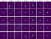 |
Fig. 1. Five examples of statistical merger sequences selected from the IllustrisTNG simulation. The exact merger time tmerger has been rounded to the nearest 0.1 Gyr. According to our default definition, pre-mergers are those with tmerger between –0.8 and –0.1 Gyr, ongoing mergers are between –0.1 and 0.1 Gyr, and post-mergers are between 0.1 and 0.3 Gyr. Galaxies that do not satisfy these conditions are defined as non-mergers. The cut-outs are 256 × 256 pixels, with a resolution of ∼0.03″ per pixel. The images were scaled using the aggressive arcsinh scaling and were then normalised. |
2.2. Realistic mock JWST images
In order to generate realistic mock JWST NIRcam F150W images, various observational effects such as spatial resolution, S/N, and background need to be included. The images from the simulation were produced with the same pixel resolution as the real JWST observations (0.03″ per pixel) and the same units of MJy/sr, and their physical size was 50 × 50 kpc. First, we convolved each image with the observed point spread function (PSF) in the F150W filter. Then, we added shot noise as Poisson noise to account for the statistical temporal variation in the photon emission of a source. Specifically, we used a randomly chosen global PSF model from the 80 models in total derived by Zhuang et al. (2023).
To make the images more realistic, we added real background from the JWST imaging data released by the COSMOS-Web programme (Casey et al. 2023) and reduced by Zhuang et al. (2023). COSMOS-Web covers the central area (0.54 deg2) of the COSMOS field (Scoville et al. 2007) in four NIRCam imaging filters (F115W, F150W, F277W, and F444W). We made image cutouts using the observed COSMOS-Web imaging data, centred on positions without artefacts or bright sources. To generate these sky cutouts, we adopted the method outlined by Margalef-Bentabol et al. (2024). First, we compiled a list of sources that were to be excluded, starting from the COSMOS2020 catalogue (Weaver et al. 2022). We used the Farmer version of COSMOS2020, applying the condition that the flag FLAG_COMBINED = 0, as recommended by the COSMOS team, to avoid areas contaminated by bright stars or large artefacts. Second, we filtered sources based on the lp_type parameter, selecting those flagged as 0 or 2 (corresponding to a galaxy or X-ray source). Third, we restricted our selection to sources at z < 3 in the COSMOS-Web field, allowing distant galaxies to be included in the cutouts. Finally, we randomly generated sky coordinates, to ensure that no catalogued sources (in the list to avoid) were present within a radius of 6.5″. This radius was determined based on the estimated source density in the region in which the cutouts were generated. As a result, these cutouts may still include background galaxies and faint sources. As the last step, we resized all images to 256 × 256 pixels. This meant that galaxies at different redshifts had slightly different pixel scales, from 0.024″ per pixel at the highest redshift to 0.032″ per pixel at the lowest redshift.
We also applied image scaling to highlight the low surface brightness details of the galaxies. First, we considered an arcsinh scaling, which reduced the dynamical range drastically, but also preserved the structures in the brighter regions (Lupton et al. 2004). We then used a more aggressive scaling, which decreased the background even further and removed any potential outlier pixels, following the approach of Bottrell et al. (2019). This was done by setting every pixel value below the median of the entire image to the median value. In addition, pixel values above the 90th percentile of the pixel intensities in the centre of the image (80 × 80 pixels in the centre) were set to this pixel value threshold. After applying image scaling, we then normalised the images,
 (1)
(1)
where x is the pixel value. The effects of the various image scaling for an example merger at z = 0.5 are shown in Fig. 2.
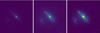 |
Fig. 2. Illustration of various scalings (left: normalised image without applying any scaling; centre: arcsinh scaling; and right: aggressive arcsinh scaling) applied to the mock JWST/NIRCam F150W images. The cut-outs are 256 × 256 pixels, with a resolution of ∼0.03″ per pixel. The images were normalised after each scaling. |
These mock JWST/NIRCAM images were used to train the merger classifier, as explained in the following section. It is generally expected that galaxy merging features are primarily driven by gravitational interactions, rather than the specific baryonic physics employed in a given simulation. A recent study (Khalid et al. 2024) focusing on tidal features fractions also qualitatively confirmed this general expectation by showing a good level of agreement among four cosmological hydrodynamical simulations.
3. Method
3.1. Zoobot
We used Zoobot, a DL-based Python package (Walmsley et al. 2023), to build and optimise an image classifier to identify merging galaxies and identify their merging stages (i.e. pre- and post-mergers). The advantage of Zoobot is that it includes models that have already been pre-trained on the GZ responses. These models can easily be adapted to solve our task. The architecture of the pre-trained model we used is called EfficientNet B0, which belongs to the family of models called EfficientNets (Tan & Le 2020). The baseline network consisted of a convolutional layer with a kernel size of 3 × 3, denoted by Conv3 × 3. The majority of the model consists of mobile inverted bottleneck MBConv blocks, which use an inverted residual block and a linear bottleneck. The last stage is a final convolutional layer, a pooling layer, and a fully connected (FC) layer. The architecture of the network is summarised in Table 1.
Baseline network.
The EfficientNet B0 model was trained on the GZ Evo dataset, as described by Walmsley et al. (2023). This dataset comes from the GZ citizen science project, where volunteers were asked questions based on morphological characteristics of galaxy images. There are various different versions of the project (Walmsley et al. 2021). Questions from many versions were used to create the GZ Evo dataset, consisting of 96.5M volunteer responses for 552k galaxy images. With this dataset, a pre-trained model was created, which was shown to have learned an internal representation capable of recognising general galaxy morphological types (Walmsley et al. 2022). Because of the generality of the representations, the resulting network is also suitable for solving new galaxy classification tasks via a method called transfer learning. As head, this model uses a linear classifier, which applies a linear transformation to the input data given by
 (2)
(2)
where x is the input data, A is the weight matrix with the shape of the input and output features, b is the bias, and y is the output data. The output dimension is the number of classes (labels) that we considered in the classification task.
To optimise the training on our own data, we first obtained the best configuration of the tunable hyperparameters. We used the grid-search approach, which can be quite time-consuming. It was important to select the parameters and settings that were to be used. Therefore, we first performed multiple episodes of random grid searches, where we provided multiple possible values from which random configurations were chosen. From the behaviour of each run, we learned more about its influences on the performance. Subsequently, for the final grid search, we were able to provide the most suitable parameters. The final grid search was performed over batch size, learning rate, weight decay, and the number of blocks that the optimiser considers to update. We present the details of the grid search in Appendix A. In Table 2, we summarise our findings for the best hyperparameter values to use for training our networks.
Final parameters used for the training of each model.
3.2. Performance metrics
We used a multi-class classification model that predicts labels on the input data. A common way to evaluate the performance of a classifier is to use the confusion matrix. Each row in a confusion matrix corresponds to the true class, and each column corresponds to the predicted class. The confusion matrix can then be used to show the number of time instances of a given true class that are classified as a given predicted class. For a perfect classifier, only the diagonal elements of the confusion matrix would have non-zero values. In order to properly compare the different classes in a confusion matrix, the result needs to be shown over a balanced test dataset (i.e. the number of instances is the same in the different true classes).
It is also common to normalise the counts in a confusion matrix. When the confusion matrix is normalised vertically, each number in the matrix is divided by the sum of the corresponding column. In this case, per predicted class the percentage that belongs to the true class can be read off, and which percentage belongs to the other classes. The same can be done horizontally and represents the percentage of each predicted class for a given true class. By normalising vertically, we derived the precision (also known as purity) of each class along the diagonal line, which is given by
 (3)
(3)
where TP (true positives) refers to the number of instances that are correctly identified to be the class of interest, and FP (false positives) refers to the number of instances that are incorrectly identified to be the class of interest. When we divide each element by the sum of the corresponding row, we obtain the recall (also known as completeness) of each class along the diagonal,
 (4)
(4)
where FN (false negatives) refers to the number of instances that are incorrectly identified to belong to the classes in which we are not interested.
Another useful metric is accuracy. This relates the performance for all the classes together. In the binary classification scenario, accuracy can be calculated as
 (5)
(5)
where TN (true negatives) is the number of instances that are correctly identified to belong to the other classes. This definition can easily be adapted to a multi-class classification scenario.
4. Results
We trained DL CNN models to identify mergers and merger stages using mock JWST NIRcam F150W images of galaxies selected from the TNG simulations. Standard data augmentation techniques, such as cropping and zooming, random rotations, and random horizontal and vertical flipping, are included in Zoobot by default. We used two different set-ups. In the first set-up, we adopted a two-stage classification, in which the first step performs a binary classification of mergers and non-mergers. The predicted mergers then go through the second step, which performs a binary classification of pre-mergers and post-mergers. The combined results from the two steps give the final three-class classifications of pre-merger, post-merger, and non-merger. In the second set-up, the three classes (i.e. non-mergers, pre-mergers, and post-mergers) are predicted simultaneously, which is referred to as the one-stage classification.
For the first model of the two-stage classification set-up, we used a dataset of 350 133 mergers and non-mergers, 81% of which was used for the training, 9% for the validation, and 10% for the testing. For the second model of the two-stage classification, 461 571 pre- and post-mergers were used, and the same training-validation-testing split was applied. For the one-stage classification set-up, we used 499 824 galaxies in total, split into 81% for the training, 9% for the validation, and 10% for the testing. A full breakdown of the number statistics can be found in Table 3.
Number statistics for the training of each model.
4.1. Overall performance
4.1.1. One-stage classification
First, we show the results of the one-stage classification for the three classes, pre-merger, post-merger, and non-mergers. From the grid search, we obtained the best values for the tuned hyper-parameters, as shown in Table 2. Using these parameters, we trained our models on the IllustrisTNG dataset, which consists of 134 763 galaxies for each of the three classes. The resulting confusion matrix from applying the trained model to the test dataset (balanced over the three classes) is shown in the top left panel in Fig. 3. Galaxies are separated into different classes based on the highest prediction score from the model. The overall accuracy of our one-stage classification set-up is 57.1% (±0.5%). The precision for the pre-merger class is 65.8%, which is much higher than the other two classes, which show precisions of about 55%. We postulate that this is probably due to the generally more recognisable and distinct features in pre-mergers, for instance, distortions in the primary galaxy, the presence of a merging companion, and interacting morphologies between the merging pair. On the other hand, recall is lowest for pre-mergers (< 50%) and much higher for the other classes (∼60% or higher). This is expected given the well-known trade-off between precision and recall. Misclassifications of pre-mergers are roughly evenly distributed in the other two classes at a level of about 25%. For post-mergers and non-mergers, confusion with the pre-merger class (at just over 10%) is significantly lower than with each other by a factor of about two. The reason probably is that post-mergers, like non-mergers, do not have a merging companion galaxy either. Several previous studies (e.g., Pearson et al. 2019b; Ćiprijanović et al. 2020; La Marca et al. 2024) have investigated which specific image features can lead to a merger classification by using techniques such as occlusion analysis and gradient-weighted class activation maps (Selvaraju et al. 2016). Generally speaking, the models rely on the presence of a merging companion and/or complex asymmetric (usually faint) features around the periphery of the central galaxy to distinguish mergers from non-mergers. To help interpret our results further, we also plot a confusion matrix corresponding to a random three-class classifier in the same set-up in the top right panel in Fig. 3. When classifications are made randomly, each class has an equal probability of being predicted, and hence, this results in precision and recall scores of approximately 33% for all classes and an overall accuracy of about 33%. In Appendix B we also directly compare the performance of our classifiers in the binary classification case (mergers versus non-mergers) with other leading merger-detection methods as presented by Margalef-Bentabol et al. (2024). The performance levels are similar overall.
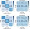 |
Fig. 3. Top left: Confusion matrix for the one-stage classification, trained and predicted on the entire dataset over all redshifts. The matrix is normalised vertically to give the precision along the diagonal. Recall is shown in brackets below (i.e. the numbers in brackets are normalised horizontally). Top right: Example confusion matrix from a random three-class classifier. Bottom left: Confusion matrix for the two-stage classification. Bottom right: Example confusion matrix from a random classifier in the two-stage set-up. For clarity, only uncertainties on the accuracy metric are shown. The uncertainties on the other metrics are broadly similar. |
4.1.2. Two-stage classification.
A similar approach was used for the two-stage classification set-up, but the grid search was made for the two steps separately. The best hyper-parameter configurations we obtained are shown in Table 2. The configuration for the model used in the second step (i.e. the pre-merger or post-merger classification) is the same as was used in the first step (i.e. the merger or non-merger classification), but we fine-tuned one additional deeper block. Furthermore, we applied class weights to both models as the data are slightly unbalanced. The model used in the first step was trained on 147 672 mergers and 134 763 non-mergers. In the second step, the two classes were initially fairly unbalanced, and pre-mergers were more numerous than post-mergers. To balance the datasets and to increase the training data, we performed data augmentation for both classes. This resulted in 186 822 pre-mergers and 184 728 post-mergers. The augmentations were made by producing new mock images from the simulated galaxy images with different backgrounds. Our test dataset was first subjected to a merger or non-merger classification. Galaxies that were predicted to be mergers were further classified into pre- and post-mergers. The results are shown in the bottom left panel in Fig. 3. The overall accuracy is 54.7% (±0.5%), which is slightly lower than that of the one-stage set-up. The precisions of the three classes are either similar to or lower than those in the one-stage classification, particularly for the non-merger class (5% lower). Again, the non-mergers and post-mergers are more strongly mixed than these two classes and the pre-merger class. In the bottom right panel in Fig. 3, we also show the results of a random classifier in the two-stage set-up. In this case, a random classifier would still give an overall accuracy of about 33% and precisions ∼33% for all classes, but the recall would be about 50% for non-mergers and 25% for pre- and post-mergers (as the test dataset is balanced over pre-mergers, post-mergers, and non-mergers).
4.1.3. Dependence on S/N.
We now analyse the effect of the S/N on the precision of the two classification set-ups. We used the photutils package (Bradley et al. 2024) to estimate the aperture photometry (within a circular aperture of 6 pixels in diameter, i.e., around 0.2″) and the background noise level within the same size area (as the dsigma-clipped standard deviation), from which we calculate the S/N. All galaxies in the dataset were binned according to their S/N over the range from 5 to 1000. We randomly chose in each S/N bin a roughly equal number of galaxies from each class, listed in Table 4. The bins up to an S/N of 100 contain approximately balanced classes between mergers and non-mergers. However, the last bin is highly unbalanced, with significantly fewer non-mergers. Next, we calculated the precision of each class in each S/N bin. The results are plotted in Fig. 4, where each horizontal line spans across the width of the S/N bin. In general, the precision levels of all three classes increase as the S/N increases for both the one-stage and two-stage set-ups, as expected. At S/N ≳ 20, the trends for pre- and post-mergers become much flatter, indicating a far weaker dependence on S/N. For the non-merger class, the precision continues to rise sharply with increasing S/N. This might partly be due to the imbalance of the three classes in the highest S/N bin, which can lead to a bias in the model predictions towards predicting merging galaxies and would result in a lower precision for both pre- and post-mergers. At any S/N bin except for the highest bin, pre-mergers have the highest precision, non-mergers have the lowest precision, and post-mergers are located in between for both set-ups.
Number of classes in each training dataset per S/N bin.
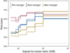 |
Fig. 4. Precision as a function of S/N for the three classes. The solid lines correspond to the one-stage classification, and the dashed lines correspond to the two-stage classification. The precision levels increase with increasing S/N, but these trends flatten at S/N ≳ 20 for pre- and post-mergers. The mean errors on the precision (derived from bootstrapping) are similar between the one-stage and two-stage set-ups and are indicated in the top left corner. The horizontal dotted line at around 33% corresponds to the precision of a random classifier. |
4.1.4. Dependence on redshift.
To examine the dependence of the model performance on redshift, we show in Fig. 5 the confusion matrices of the model trained on all redshifts, but predicted separately for each redshift bin. As expected, in both set-ups that predict lower-z galaxies, the precision, recall, and accuracy for all classes is generally higher because typically, lower-z galaxies are larger and have a higher S/N. Again, the one-stage set-up generally has a better precision, particularly for non-mergers. Since the two-stage classification set-up depends on two steps, we also present the performance of the two separate models per redshift range in Table 5. In the first step, the recall of the non-merger class decreases much more quickly than for the merger class. At 0 ≤ z < 1, the recall is 80% and 64% for the non-mergers and mergers, respectively. At 2 ≤ z < 3, the recall is reduced by 14% for the non-mergers and by only 4% for the mergers. On the other hand, the precision of the mergers is much more affected by redshift than that of the non-mergers. This ultimately results in more FP (i.e. non-mergers classified as mergers) at higher-z, and it therefore contaminates the second step of the classification. To analyse the results from the second step, we only considered the TPs (i.e. correctly identified mergers) from the first step. A significant decline in recall is only found in the pre-mergers. However, the precision declines more sharply for the post-mergers. As discussed previously, this might partially be due to the number distribution of the different classes in the high-z bin (lowest S/N bin), which is mainly dominated by post-mergers. In a separate experiment, we also trained the classifiers in each redshift bin separately. However, as the numbers of galaxies used for training decreased by a factor of 10 in the highest-redshift bin, the results did not improve much.
Precision and recall score of the two steps of the two-stage classification.
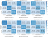 |
Fig. 5. Confusion matrix of the one-stage (top row) and two-stage (bottom row) predicted per redshift range (left: 0 ≤ z < 1; middle: 1 ≤ z < 2; right: 2 ≤ z < 3). All matrices are vertically normalised. The recall is shown below in brackets. |
To summarise, the one-stage classification set-up moderately outperforms the two-stage set-up as it offers a better accuracy and precision. The recall of the one-stage set-up for the non-merger class is worse than that of the two-stage set-up. However, the precision is usually more important than recall for merger studies. In addition, mergers are relatively rare, and a lower recall in the non-mergers class is therefore not an issue as far as the sample size is concerned. The one-stage set-up might outperform the two-stage set-up because it can be more difficult for DL models to identify a class that consists of a mix of morphologies types. A set-up that places more similar galaxies in a finer classification system can be helpful for the DL models to learn the (sometimes very) subtle differences between the various classes better.
4.2. Dependence on the merger time
During the billion-year-long galaxy merging processes, merging features clearly evolve as the galaxies interact with each other. Some merging stages associated with clear and distinct signs such as tidal tails and bridges can be easier to identify than other stages. We wish to understand how the merger time tmerger before or after the coalescence event affects the prediction scores of each class, with a focus on the boundaries between the different classes.
Fig. 6 shows the recall of the three classes against merger time tmerger for the two set-ups. The pink (blue) shaded region corresponds to the regime of the true pre-mergers (post-mergers), and the white regions correspond to the regime of the true non-mergers. In general, the recall levels for both pre- and post-mergers increase when these mergers are closer to the coalescence event. This indicates that it is easier to detect them, possibly due to more conspicuous features. At the boundary between pre-mergers and post-mergers, the recall is significantly decreased, which is expected because the two classes are more strongly mixed at the boundary. For non-mergers, the recall increases for galaxies with more distant merging events in their past or future evolutionary histories because these galaxies are likely to have more regular morphologies. The one-stage classification set-up results in a higher recall for mergers, particularly for post-mergers. In the two-stage set-up, the two merger classes are predicted via two networks and therefore have a higher likelihood of being polluted by other classes. For non-mergers, the two-stage set-up has a higher recall than the one-stage set-up. This is to be expected as the precision of the non-mergers in the two-stage set-up is worse than in the one-stage set-up. Another point to keep in mind is that the recall of a random classifier in the two-stage set-up is about 50%. Therefore, the overall recall of the non-merger class in the two-stage set-up, at about 75% (as shown in Fig. 3), is 25% points better than random classifications. In comparison, the overall recall of the non-merger class in the one-stage set-up, at about 65%, is ∼30% better than that from a random classifier in the one-stage set-up.
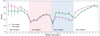 |
Fig. 6. Recall of each class as a function of merger time before or after the coalescence (one-stage: green solid line, and two-stage: purple dashed line). The x-axis is stretched in the merger regime. The blue shaded area corresponds to the true post-merger regime, the pink shaded area corresponds to the true pre-merger region, and the white area is the true non-merger regime. The error bars are derived from the bootstrap error. |
In Fig. 7 we plot the fraction of each predicted class versus tmerger. In the post-merger regime, a perfect classifier would return 100% for the predicted post-mergers and 0% for the predicted pre-mergers and non-mergers. For both the one-stage and two-stage set-ups, the fraction of the predicted post-mergers decreases with increasing merger time after coalescence. This indicates that the classifiers are more strongly mixed, probably due to the vanishing merging features. For the two-stage set-up, galaxies are even more likely to be classified as non-mergers at tmerger > 0.15 Gyr. In comparison, in the one-stage set-up, the fraction of the predicted post-mergers is much higher and the fraction of the predicted non-mergers is much lower. This implies that this set-up distinguishes post-mergers and non-mergers better. In the pre-merger regime, both set-ups show similar fractions of predicted pre-mergers, which generally decrease with increasingly negative merger times (coalescence is farther away in the future). Both set-ups perform well in the region from about tmerger = −0.2 up to –0.5 Gyr. Beyond tmerger = −0.5 Gyr, the fraction of predicted non-mergers is higher than that of the predicted pre-mergers in the two-stage set-up. In comparison, the fraction of the predicted non-mergers does not overtake that of the predicted pre-mergers until about tmerger = −0.7 Gyr in the one-stage set-up. In the non-merger regime, the two-stage set-up returns a higher fraction of predicted non-mergers than the one-stage set-up. This is related to the fact that the one-stage set-up has a higher precision for the non-merger class, which generally means that the recall will be lower.
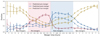 |
Fig. 7. Fraction of the three predicted classes as a function of merger time before or after coalescence in the regimes of true mergers (blue shaded region: true post-mergers, and pink shaded region: true pre-mergers) and true non-mergers. The x-axis is stretched in the merger regime. The solid lines indicate the results of the one-stage classification set-up. The dashed lines indicate the results of the two-stage classification set-up. The error bars are derived from bootstrap error. For a perfect classifier, the fraction of predicted pre-mergers, post-mergers, or non-mergers would be 100% in the true pre-merger, post-merger, or non-merger region and 0% everywhere else. |
We investigated how confident the classifier is as a function of tmerger, which is reflected in the prediction scores that the model gives to each class. For each galaxy, the highest score determined the predicted label. If the model is very confident, the prediction score of a particular class is much higher than for the other classes. In Fig. 8 we plot the average pre-, post-, and non-merger prediction scores as a function of tmerger. For the two-stage set-up, the first model gives a merger score and non-merger score. The second model gives a pre-merger score and post-merger score, which are only given to galaxies with a merger score > 0.5 from the previous stage. Non-mergers predicted as mergers in the first stage are therefore classified as pre- or post-merger in the second stage. Hence, one of these scores could be very high, even though the original merger score was perhaps fairly low. For the two-stage set-up, the highest average score for a merger is in the true pre-merger regime, particularly in the range tmerger = −0.5 to –0.1 Gyr. The merger scores are generally significantly lower in the true post-merger regime than in the true pre-merger regime. This implies that for post-mergers, the first stage is the main problem for misclassifications. This confusion is much lower in the one-stage classification set-up. When we compare the true non-merger regimes in the two set-ups, the non-merger prediction score decreases towards the boundaries with true pre- and post-mergers.
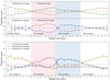 |
Fig. 8. Prediction score as a function of merger time (top panel: the two-stage classification set-up, and bottom panel: the one-stage set-up). The x-axis is stretched in the merger regime. In the two-stage set-up, the first stage gives each galaxy a merger (green) and non-merger (yellow) prediction score. For the predicted mergers, the second stage gives a pre-merger (purple) and post-merger (blue) prediction score. The error bars correspond to the bootstrap errors. For the one-stage (two-stage) set-up, a grey dotted line at 0.33 (0.5) is added to indicate the prediction score of a random classifier. |
4.3. Retraining the network
In Sect. 4.2 we showed that the performance metrics of the classifiers and the confidence levels of their predictions depend sensitively on the merger time tmerger since or before the coalescence. In general, the classifiers give a better precision, recall, and higher confidence for mergers that are caught closer to the actual merging event. In our default definition of pre-mergers, we used a relatively long time range between tmerger = −0.8 and –0.1 Gyr. Therefore, for the pre-merger class we would like to confirm whether it is better to select a different boundary by changing the definition of the pre-merger and non-merger class, and we then retrained the two classification set-ups for each new definition.
We considered new boundaries at tmerger = −0.7, −0.6, −0.5, −0.4, −0.3, −0.2, and –0.1 Gyr. Pre-mergers outside the new definition window were now labelled as non-mergers. For example, a pre-merger that was located along the merging sequence at tmerger = −0.65 Gyr was initially defined as a pre-merger. When we changed the definition of pre-mergers using a new boundary at tmerger = −0.6 Gyr, this galaxy was then labelled as a non-merger. In terms of the overall accuracy for the three classes, we found that the highest overall accuracy for the two-stage (one-stage) set-up, 58.4% (59.4%), is achieved when tmerger = 0.2 (0.4) Gyr was adopted. This finding supports our previous conclusion that the one-stage set-up generally performs better than the two-stage set-up, with a better accuracy and a wider range in merger time.
In Fig. 9 we plot the precision and recall as a function of the boundary set between pre-mergers and non-mergers for the two classification set-ups. For the two metrics, pre-mergers are clearly affected most when the boundary changed, which is expected as the other two classes (post-mergers and non-mergers) are not much affected. The precision levels of the pre-mergers continue to rise with the focus on pre-mergers, which are located closer to the actual merging event, for the two classification set-ups, from about 65% at tmerger = −0.8 Gyr (the original definition) to about 72% at tmerger = −0.2 Gyr. Similarly, the recall levels of the pre-mergers also generally improve from tmerger = −0.8 to –0.2 Gyr, but these trends flatten more or less at about tmerger = −0.4 Gyr. When we take all the classes into account, the best definition of pre-merger would be galaxies that will under go a merger event in the following 0.4 Gyr. The results from the model trained with this definition improved for the majority of classes in terms of both precision and recall.
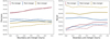 |
Fig. 9. Precision (left) and recall (right) scores of the three classes as a function of the new pre-merger definition. The solid lines represent the one-stage classification, and the dashed lines represent the two-stage classification. The error bars derived from the bootstrapping are similar for the one-stage and two-stage set-ups. The mean errors for the three classes are indicated at the top. |
5. Conclusion
We used advanced DL models as implemented in the Zoobot Python package to detect non-mergers and mergers, including their merger stages in mock JWST/NIRCam F150W images of simulated galaxies over the redshift range 0.5 ≤ z ≤ 3.0 selected from the IllustrisTNG cosmological hydrodynamical simulations. We employed two classification set-ups, that is, one-stage versus two-stage classification, to test whether it is more advantageous to detect mergers and merger stages in a hierarchical fashion or simultaneously. We also investigated the change in the performance of our classifiers as a function of S/N, redshift, and merger time relative to the merging event. Our main findings are listed below.
-
The one-stage classification set-up that identifies mergers and their merger stages simultaneously generally performs better than the hierarchical two-stage set-up. It yields a higher overall accuracy and generally better precision (particularly for the non-merger class). In terms of recall, the one-stage set-up performs better for pre- and post-mergers, but worse for non-mergers. However, this is partly due to the trade-off between precision and recall. For merger studies, we generally prioritise precision over recall. Therefore, we recommend the one-stage set-up for the identification of mergers and their merger stages.
-
Pre-mergers are classified with the highest precision. The mix between the post-mergers and non-mergers is stronger than between these two classes and the pre-merger class. This is expected because pre-mergers can have more recognisable features, for instance, a companion galaxy in addition to the distorted morphologies in the primary galaxy.
-
The precision of the DL classifiers generally improved with increasing S/N. The trends are particularly steep at the faint end and then flatten towards higher S/N. Therefore, it is important for studies involving merger detections to first investigate the dependence on S/N and then choose an optimal threshold to balance the performance and sample size.
-
The performance of the classifiers depends on the exact merger stage in terms of time since or before the merging event (i.e. coalescence). The precision continues to increase for pre-mergers closer to coalescence, but the recall plateaus at about tmerger = −0.4 Gyr. To maintain a good balance between the precision and recall and also consider the sample size, we therefore recommend using a cut at –0.4 Gyr to select pre-mergers.
In our future work, we will explore the connection between key galaxy evolutionary phases (e.g. the triggering of starburst activities and accretion onto SMBHs) and merger stages in real JWST data. For example, we will address whether the starburst phase is more likely to be activated in the pre-merger stage and the SMBH accretion more likely to be triggered in the post-merger stage according to the one-stage classification set-up and the recommended cuts on S/N and merger time from this paper. In this paper, we investigated merger stages at the most basic level, that is, we separated mergers into pre- and post-mergers. Another future direction would be to refine the time resolution by determining mergers along their merging sequences.
Acknowledgments
This publication is part of the project ‘Clash of the Titans: deciphering the enigmatic role of cosmic collisions’ (with project number VI.Vidi.193.113 of the research programme Vidi which is (partly) financed by the Dutch Research Council (NWO). We thank the Center for Information Technology of the University of Groningen for their support and for providing access to the Hábrók high-performance computing cluster. We thank SURF (www.surf.nl) for the support in using the National Supercomputer Snellius. W.J.P. has been supported by the Polish National Science Center project UMO-2023/51/D/ST9/00147. The Dunlap Institute is funded through an endowment established by the David Dunlap family and the University of Toronto.
References
- Ackermann, S., Schawinski, K., Zhang, C., Weigel, A. K., & Turp, M. D. 2018, MNRAS, 479, 415 [NASA ADS] [CrossRef] [Google Scholar]
- Aihara, H., Arimoto, N., Armstrong, R., et al. 2018, PASJ, 70, S4 [NASA ADS] [Google Scholar]
- Bickley, R. W., Bottrell, C., Hani, M. H., et al. 2021, MNRAS, 504, 372 [NASA ADS] [CrossRef] [Google Scholar]
- Biewald, L. 2020, Experiment Tracking with Weights and Biases, https://www.wandb.com/ [Google Scholar]
- Blecha, L., Snyder, G. F., Satyapal, S., & Ellison, S. L. 2018, MNRAS, 478, 3056 [Google Scholar]
- Blumenthal, K. A., Moreno, J., Barnes, J. E., et al. 2020, MNRAS, 492, 2075 [CrossRef] [Google Scholar]
- Bottrell, C., Hani, M. H., Teimoorinia, H., et al. 2019, MNRAS, 490, 5390 [NASA ADS] [CrossRef] [Google Scholar]
- Bradley, L., Sipőcz, B., Robitaille, T., et al. 2024, https://doi.org/10.5281/zenodo.12585239 [Google Scholar]
- Bruzual, G., & Charlot, S. 2003, MNRAS, 344, 1000 [NASA ADS] [CrossRef] [Google Scholar]
- Byrne-Mamahit, S., Patton, D. R., Ellison, S. L., et al. 2024, MNRAS, 528, 5864 [Google Scholar]
- Casey, C. M., Kartaltepe, J. S., Drakos, N. E., et al. 2023, ApJ, accepted [arXiv:2211.07865] [Google Scholar]
- Ćiprijanović, A., Snyder, G. F., Nord, B., & Peek, J. E. G. 2020, Astron. Comput., 32, 100390 [CrossRef] [Google Scholar]
- Ćiprijanović, A., Kafkes, D., Downey, K., et al. 2021, MNRAS, 506, 677 [CrossRef] [Google Scholar]
- Cole, S., Lacey, C. G., Baugh, C. M., & Frenk, C. S. 2000, MNRAS, 319, 168 [Google Scholar]
- Conselice, C. J. 2003, ApJS, 147, 1 [NASA ADS] [CrossRef] [Google Scholar]
- Conselice, C. J., Bershady, M. A., & Jangren, A. 2000, ApJ, 529, 886 [NASA ADS] [CrossRef] [Google Scholar]
- Conselice, C. J., Bershady, M. A., Dickinson, M., & Papovich, C. 2003, AJ, 126, 1183 [CrossRef] [Google Scholar]
- Conselice, C. J., Mundy, C. J., Ferreira, L., & Duncan, K. 2022, ApJ, 940, 168 [CrossRef] [Google Scholar]
- Darg, D. W., Kaviraj, S., Lintott, C. J., et al. 2010, MNRAS, 401, 1043 [NASA ADS] [CrossRef] [Google Scholar]
- Deng, J., Dong, W., Socher, R., et al. 2009, in 2009 IEEE Conference on Computer Vision and Pattern Recognition, 248 [CrossRef] [Google Scholar]
- Dieleman, S., Willett, K. W., & Dambre, J. 2015, MNRAS, 450, 1441 [NASA ADS] [CrossRef] [Google Scholar]
- Donnari, M., Pillepich, A., Nelson, D., et al. 2019, MNRAS, 485, 4817 [Google Scholar]
- Duan, Q., Conselice, C. J., Li, Q., et al. 2025, MNRAS, submitted [arXiv:2407.09472] [Google Scholar]
- Dubois, Y., Pichon, C., Welker, C., et al. 2014, MNRAS, 444, 1453 [Google Scholar]
- Duncan, K., Conselice, C. J., Mundy, C., et al. 2019, ApJ, 876, 110 [NASA ADS] [CrossRef] [Google Scholar]
- Ellison, S. L., Patton, D. R., Simard, L., & McConnachie, A. W. 2008, AJ, 135, 1877 [NASA ADS] [CrossRef] [Google Scholar]
- Ellison, S. L., Viswanathan, A., Patton, D. R., et al. 2019, MNRAS, 487, 2491 [NASA ADS] [CrossRef] [Google Scholar]
- Ferreira, L., Conselice, C. J., Duncan, K., et al. 2020, ApJ, 895, 115 [NASA ADS] [CrossRef] [Google Scholar]
- Ferreira, L., Bickley, R. W., Ellison, S. L., et al. 2024, MNRAS, 533, 2547 [NASA ADS] [CrossRef] [Google Scholar]
- Gao, F., Wang, L., Pearson, W. J., et al. 2020, A&A, 637, A94 [NASA ADS] [CrossRef] [EDP Sciences] [Google Scholar]
- Gardner, J. P., Mather, J. C., Clampin, M., et al. 2006, Space Sci. Rev., 123, 485 [Google Scholar]
- Goodfellow, I., Bengio, Y., & Courville, A. 2016, Deep Learning (MIT Press), http://www.deeplearningbook.org [Google Scholar]
- Goulding, A. D., Greene, J. E., Bezanson, R., et al. 2018, PASJ, 70, S37 [NASA ADS] [CrossRef] [Google Scholar]
- Helmi, A. 2020, ARA&A, 58, 205 [Google Scholar]
- Hopkins, P. F., Hernquist, L., Cox, T. J., & Kereš, D. 2008, ApJS, 175, 356 [Google Scholar]
- Huertas-Company, M., & Lanusse, F. 2023, PASA, 40, e001 [NASA ADS] [CrossRef] [Google Scholar]
- Huertas-Company, M., Gravet, R., Cabrera-Vives, G., et al. 2015, ApJS, 221, 8 [NASA ADS] [CrossRef] [Google Scholar]
- Kartaltepe, J. S., Mozena, M., Kocevski, D., et al. 2015, ApJS, 221, 11 [NASA ADS] [CrossRef] [Google Scholar]
- Khalid, A., Brough, S., Martin, G., et al. 2024, MNRAS, 530, 4422 [Google Scholar]
- Knapen, J. H., Cisternas, M., & Querejeta, M. 2015, MNRAS, 454, 1742 [NASA ADS] [CrossRef] [Google Scholar]
- Krizhevsky, A., Sutskever, I., & Hinton, G. 2012, Adv. Neural Inf. Process. Syst., 25, 1097 [Google Scholar]
- La Marca, A., Margalef-Bentabol, B., Wang, L., et al. 2024, A&A, 690, A326 [NASA ADS] [CrossRef] [EDP Sciences] [Google Scholar]
- Lambas, D. G., Alonso, S., Mesa, V., & O’Mill, A. L. 2012, A&A, 539, A45 [NASA ADS] [CrossRef] [EDP Sciences] [Google Scholar]
- Lecun, Y., Bottou, L., Bengio, Y., & Haffner, P. 1998, Proc. IEEE, 86, 2278 [Google Scholar]
- Li, R., Napolitano, N. R., Tortora, C., et al. 2020, ApJ, 899, 30 [Google Scholar]
- Liao, S., Johansson, P. H., Mannerkoski, M., et al. 2023, MNRAS, 520, 4463 [Google Scholar]
- Lintott, C. J., Schawinski, K., Slosar, A., et al. 2008, MNRAS, 389, 1179 [NASA ADS] [CrossRef] [Google Scholar]
- Lintott, C., Schawinski, K., Bamford, S., et al. 2011, MNRAS, 410, 166 [Google Scholar]
- Lotz, J. M., Primack, J., & Madau, P. 2004, AJ, 128, 163 [NASA ADS] [CrossRef] [Google Scholar]
- Lotz, J. M., Davis, M., Faber, S. M., et al. 2008, ApJ, 672, 177 [NASA ADS] [CrossRef] [Google Scholar]
- Lotz, J. M., Jonsson, P., Cox, T. J., et al. 2011, ApJ, 742, 103 [Google Scholar]
- Lupton, R., Blanton, M., Fekete, G., et al. 2004, PASP, 116, 133 [NASA ADS] [CrossRef] [Google Scholar]
- Margalef-Bentabol, B., Wang, L., La Marca, A., et al. 2024, A&A, 687, A24 [NASA ADS] [CrossRef] [EDP Sciences] [Google Scholar]
- Marinacci, F., Vogelsberger, M., Pakmor, R., et al. 2018, MNRAS, 480, 5113 [NASA ADS] [Google Scholar]
- Naiman, J. P., Pillepich, A., Springel, V., et al. 2018, MNRAS, 477, 1206 [Google Scholar]
- Nelson, D., Pillepich, A., Springel, V., et al. 2017, MNRAS, 475, 624 [Google Scholar]
- Nelson, D., Springel, V., Pillepich, A., et al. 2019, Comput. Astrophys. Cosmol., 6, 2 [Google Scholar]
- Nelson, D., Springel, V., Pillepich, A., et al. 2021, arXiv e-prints [arXiv:1812.05609] [Google Scholar]
- Patton, D. R., Ellison, S. L., Simard, L., McConnachie, A. W., & Mendel, J. T. 2011, MNRAS, 412, 591 [NASA ADS] [CrossRef] [Google Scholar]
- Pearson, W. J., Wang, L., Alpaslan, M., et al. 2019a, A&A, 631, A51 [NASA ADS] [CrossRef] [EDP Sciences] [Google Scholar]
- Pearson, W. J., Wang, L., Trayford, J. W., Petrillo, C. E., & van der Tak, F. F. S. 2019b, A&A, 626, A49 [NASA ADS] [CrossRef] [EDP Sciences] [Google Scholar]
- Pearson, W. J., Suelves, L. E., Ho, S. C. C., et al. 2022, A&A, 661, A52 [NASA ADS] [CrossRef] [EDP Sciences] [Google Scholar]
- Pearson, W. J., Rodriguez-Gomez, V., Kruk, S., & Margalef-Bentabol, B. 2024, A&A, 687, A45 [NASA ADS] [CrossRef] [EDP Sciences] [Google Scholar]
- Petrillo, C. E., Tortora, C., Chatterjee, S., et al. 2017, MNRAS, 472, 1129 [Google Scholar]
- Pillepich, A., Nelson, D., Hernquist, L., et al. 2017, MNRAS, 475, 648 [Google Scholar]
- Planck Collaboration XIII. 2016, A&A, 594, A13 [NASA ADS] [CrossRef] [EDP Sciences] [Google Scholar]
- Quai, S., Byrne-Mamahit, S., Ellison, S. L., Patton, D. R., & Hani, M. H. 2023, MNRAS, 519, 2119 [Google Scholar]
- Rieke, M. J., Kelly, D. M., Misselt, K., et al. 2023, PASP, 135, 028001 [CrossRef] [Google Scholar]
- Rodriguez-Gomez, V., Genel, S., Vogelsberger, M., et al. 2015, MNRAS, 449, 49 [Google Scholar]
- Rodríguez Montero, F., Davé, R., Wild, V., Anglés-Alcázar, D., & Narayanan, D. 2019, MNRAS, 490, 2139 [CrossRef] [Google Scholar]
- Satyapal, S., Ellison, S. L., McAlpine, W., et al. 2014, MNRAS, 441, 1297 [Google Scholar]
- Schaefer, C., Geiger, M., Kuntzer, T., & Kneib, J. P. 2018, A&A, 611, A2 [NASA ADS] [CrossRef] [EDP Sciences] [Google Scholar]
- Schaye, J., Crain, R. A., Bower, R. G., et al. 2015, MNRAS, 446, 521 [Google Scholar]
- Scoville, N., Aussel, H., Brusa, M., et al. 2007, ApJS, 172, 1 [Google Scholar]
- Selvaraju, R. R., Cogswell, M., Das, A., et al. 2016, arXiv e-prints [arXiv:1610.02391] [Google Scholar]
- Snyder, G. F., Rodriguez-Gomez, V., Lotz, J. M., et al. 2019, MNRAS, 486, 3702 [NASA ADS] [CrossRef] [Google Scholar]
- Springel, V., Pakmor, R., Pillepich, A., et al. 2017, MNRAS, 475, 676 [Google Scholar]
- Tan, M., & Le, Q. V. 2020, arXiv e-prints [arXiv:1905.11946] [Google Scholar]
- Villforth, C. 2023, Open J. Astrophys., 6, 34 [NASA ADS] [CrossRef] [Google Scholar]
- Vogelsberger, M., Genel, S., Springel, V., et al. 2014, MNRAS, 444, 1518 [Google Scholar]
- Walmsley, M., Lintott, C., Géron, T., et al. 2021, MNRAS, 509, 3966 [NASA ADS] [CrossRef] [Google Scholar]
- Walmsley, M., Lintott, C., Géron, T., et al. 2022, MNRAS, 509, 3966 [Google Scholar]
- Walmsley, M., Allen, C., Aussel, B., et al. 2023, J. Open Source Softw., 8, 5312 [NASA ADS] [CrossRef] [Google Scholar]
- Wang, L., Pearson, W. J., & Rodriguez-Gomez, V. 2020, A&A, 644, A87 [NASA ADS] [CrossRef] [EDP Sciences] [Google Scholar]
- Weaver, J. R., Kauffmann, O. B., Ilbert, O., et al. 2022, ApJS, 258, 11 [NASA ADS] [CrossRef] [Google Scholar]
- White, S. D. M., & Frenk, C. S. 1991, ApJ, 379, 52 [Google Scholar]
- Zanisi, L., Huertas-Company, M., Lanusse, F., et al. 2021, MNRAS, 501, 4359 [NASA ADS] [CrossRef] [Google Scholar]
- Zhuang, M. Y., Li, J., & Shen, Y. 2023, ApJ, submitted [arXiv:2309.03266] [Google Scholar]
Appendix A: Hyper-parameter tuning
The final grid search was performed over batch size, learning rate, weight decay, and the number of blocks that the optimiser will consider to update. For each grid search, only a subset of the complete catalogue at low redshifts (z = 0.5) was considered to reduce computation time. In total, we did three grid searches: one to train the model of the one-stage classification set-up, and two to train the models used for the two-stage classification set-up. The parameters considered for each grid search can be found in Table A.1. The grid search was created and performed via the Weights & Biases (WandB) platform (Biewald 2020). This artificial intelligence (AI) developer platform not only provides an interface to create and initiate the grid search on, but also tracks the performance metrics for each run. In the WandB interface, the performance metrics are plotted for both the validation and training data as a function of epoch. We choose to present in this paper only the accuracy performance metric, but recall and precision were also considered during the decision making process on the hyperparameter search.
The grid search for the first model of the two-stage set-up (i.e. the merger or non-merger classification), resulted in 44 runs. It is visually difficult to distinguish each run and conclude which configuration is best. Fortunately, WandB provides multiple solutions that help identifying the effect that each parameter has. Instead of looking at all configurations simultaneously, it is also possible to group the runs on a specific parameter. For instance, if we group by batch size, which in our case has two values, then the results are two plots with one showing the average performance over all runs consisting of the first value and the other showing the average performance over all runs consisting of the other value. From this average behaviour, we can identify the influence that a given parameter has on the learning curve. Another useful tool provided by WandB is the filter. Once we have established that a particular value works best for a specific hyperparameter, we are not interested anymore in the runs consisting of a different value. Using WandB’s filter function, we can extract only those runs we are interested in.
Hyperparameter settings for each grid search.
For the merger or non-merger classification we first grouped the runs based on learning rate. The top panel in Fig. A.1 shows the accuracy of the training data and validation data for runs with learning rate of 1e − 4 and 1e − 5. At first, it seem that the higher learning rate performs better. However, when focusing only on the validation data, one can see that they reach the same accuracy. This indicates that a higher learning rate will tend to overfit. Therefore, we filtered out all runs with higher learning rates. The same trend is seen in the pre-and post-merger classification model, which we do not visualise here. Next we grouped the runs on batch size, as shown in the second panel (from the top) in Fig. A.1. For the validation dataset, runs with different batch sizes reach similar accuracies. For the training dataset, the batch size of 64 is slightly better. As we want to keep performance for the training and validation datasets as close as possible to reduce overfitting, a batch size of 128 is better. Note that for the batch size we discussed the merger or non-merger classification only. The pre-merger or post-merger classification did not show any clear preference. Since for the two-stage set-up we combine the two models of each stage, we decided to keep the parameters for both stages the same.
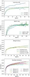 |
Fig. A.1. Accuracy scores of the merger or non-merger classification versus epoch during the training phase. The first and second panels from the top are the result of the grid search performed on galaxies at low redshifts. The third and fourth panels from the top are the results of training on the entire dataset ranging from z = 0 to 3. The title of each panel indicates the parameter which the runs are grouped on. In other words, each panel shows the average scores of all runs containing the parameter values shown in the legend. From top to bottom, grid searches are grouped on the learning rate, batch size, weight decay, and number of blocks tuned. The solid lines correspond to the training set and the dashed lines correspond to the validation set. |
For the last two parameters we did separate runs on the complete dataset over the redshift range 0.5 < z < 3 as the grid search did not provide any clear distinction. Changing the weight decay parameter from the default (0.05) had no influence on the training. The most apparent impact on the performance is the number of epochs it takes to reach the stopping criteria. Increasing the weight decay lead to an early-stopping. However, it would need more epochs during training to reach the accuracy of the other runs with lower weight decay, as demonstrated in the third panel (from the top) in Fig. A.1. Therefore, we decided to use the default value. We also performed various runs in which, with each run, we fine-tuned one deeper block. Fine-tuning up to block 3, 4, 5, 6 and 7 is shown in the bottom panel in Fig. A.1. The highest accuracy is achieved when increasing the number of blocks to perform the fine-tuning on. However, finetuning on more blocks increases computation time. Therefore, we chose to finetune 4 blocks in the first stage model, and 5 blocks in the second model. Lastly, we also performed two runs for the two scaling methods as discussed in Sect. 2.2. The resulting two runs are shown in Fig. A.2. We conclude that the aggressive arcsinh scaling leads to higher accuracies. The plots resulted only from the grid search and some consecutive runs done on the first model in the two-stage classification. For the results of the other two models we have used the same procedure. In general, the same trends among the parameters were seen in all runs.
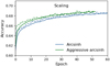 |
Fig. A.2. Separate runs performed on the scaling while leaving the other hyperparameters the same. The blue lines correspond to the simple arcsinh scaling, while the green lines used a more aggressive arcsinh scaling which decreases the presence of the background further. The solid lines correspond to the training set and the dashed lines correspond to the validation set. |
Appendix B: Binary classification: Merger versus non-merger
In Margalef-Bentabol et al. (2024), six leading ML or DL based merger detection methods were bench-marked using the same datasets, which include mock observations from the IllustrisTNG simulations, mock observations from the Horizon-AGN simulations and real observations from the HSC-SSP survey. In the redshift range 0.52 ≤ z ≤ 0.76, the precision for the merger class achieved by these methods on the TNG-test dataset ranges between 68.1% to 78.6% and the recall for the merger class ranges between 66.4% and 84.1%. In the redshift range 0.76 ≤ z ≤ 1, precision ranges between 68.2% to 75.7% and recall ranges between 57.5% to 76.2%.
To directly compare with the performances achieved in Margalef-Bentabol et al. (2024), we combined our pre- and post-merger classes into a single merger class and re-calculated the performance metrics of our classifiers in the binary classification case (i.e., mergers versus. non-mergers). In Fig. B.1, we show the confusion matrices for binary classification from our one-stage and two-stage classification set-ups. It is clear that our classifiers presented in this paper achieve similar performance to the methods presented in Margalef-Bentabol et al. (2024).
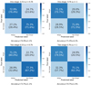 |
Fig. B.1. Top left: Confusion matrix for the one-stage classification in the binary classification case (i.e., mergers versus non-mergers), predicted on the dataset in the redshift range 0.52 ≤ z ≤ 0.76. Top right: Similar to the top left figure but for 0.76 ≤ z ≤ 1. Bottom left: Confusion matrix for the two-stage classification in the binary classification case, in the redshift range 0.52 ≤ z ≤ 0.76. Bottom right: Similar to the bottom left figure but for 0.76 ≤ z ≤ 1. |
All Tables
All Figures
|
Fig. 1. Five examples of statistical merger sequences selected from the IllustrisTNG simulation. The exact merger time tmerger has been rounded to the nearest 0.1 Gyr. According to our default definition, pre-mergers are those with tmerger between –0.8 and –0.1 Gyr, ongoing mergers are between –0.1 and 0.1 Gyr, and post-mergers are between 0.1 and 0.3 Gyr. Galaxies that do not satisfy these conditions are defined as non-mergers. The cut-outs are 256 × 256 pixels, with a resolution of ∼0.03″ per pixel. The images were scaled using the aggressive arcsinh scaling and were then normalised. |
| In the text | |
|
Fig. 2. Illustration of various scalings (left: normalised image without applying any scaling; centre: arcsinh scaling; and right: aggressive arcsinh scaling) applied to the mock JWST/NIRCam F150W images. The cut-outs are 256 × 256 pixels, with a resolution of ∼0.03″ per pixel. The images were normalised after each scaling. |
| In the text | |
|
Fig. 3. Top left: Confusion matrix for the one-stage classification, trained and predicted on the entire dataset over all redshifts. The matrix is normalised vertically to give the precision along the diagonal. Recall is shown in brackets below (i.e. the numbers in brackets are normalised horizontally). Top right: Example confusion matrix from a random three-class classifier. Bottom left: Confusion matrix for the two-stage classification. Bottom right: Example confusion matrix from a random classifier in the two-stage set-up. For clarity, only uncertainties on the accuracy metric are shown. The uncertainties on the other metrics are broadly similar. |
| In the text | |
|
Fig. 4. Precision as a function of S/N for the three classes. The solid lines correspond to the one-stage classification, and the dashed lines correspond to the two-stage classification. The precision levels increase with increasing S/N, but these trends flatten at S/N ≳ 20 for pre- and post-mergers. The mean errors on the precision (derived from bootstrapping) are similar between the one-stage and two-stage set-ups and are indicated in the top left corner. The horizontal dotted line at around 33% corresponds to the precision of a random classifier. |
| In the text | |
|
Fig. 5. Confusion matrix of the one-stage (top row) and two-stage (bottom row) predicted per redshift range (left: 0 ≤ z < 1; middle: 1 ≤ z < 2; right: 2 ≤ z < 3). All matrices are vertically normalised. The recall is shown below in brackets. |
| In the text | |
|
Fig. 6. Recall of each class as a function of merger time before or after the coalescence (one-stage: green solid line, and two-stage: purple dashed line). The x-axis is stretched in the merger regime. The blue shaded area corresponds to the true post-merger regime, the pink shaded area corresponds to the true pre-merger region, and the white area is the true non-merger regime. The error bars are derived from the bootstrap error. |
| In the text | |
|
Fig. 7. Fraction of the three predicted classes as a function of merger time before or after coalescence in the regimes of true mergers (blue shaded region: true post-mergers, and pink shaded region: true pre-mergers) and true non-mergers. The x-axis is stretched in the merger regime. The solid lines indicate the results of the one-stage classification set-up. The dashed lines indicate the results of the two-stage classification set-up. The error bars are derived from bootstrap error. For a perfect classifier, the fraction of predicted pre-mergers, post-mergers, or non-mergers would be 100% in the true pre-merger, post-merger, or non-merger region and 0% everywhere else. |
| In the text | |
|
Fig. 8. Prediction score as a function of merger time (top panel: the two-stage classification set-up, and bottom panel: the one-stage set-up). The x-axis is stretched in the merger regime. In the two-stage set-up, the first stage gives each galaxy a merger (green) and non-merger (yellow) prediction score. For the predicted mergers, the second stage gives a pre-merger (purple) and post-merger (blue) prediction score. The error bars correspond to the bootstrap errors. For the one-stage (two-stage) set-up, a grey dotted line at 0.33 (0.5) is added to indicate the prediction score of a random classifier. |
| In the text | |
|
Fig. 9. Precision (left) and recall (right) scores of the three classes as a function of the new pre-merger definition. The solid lines represent the one-stage classification, and the dashed lines represent the two-stage classification. The error bars derived from the bootstrapping are similar for the one-stage and two-stage set-ups. The mean errors for the three classes are indicated at the top. |
| In the text | |
|
Fig. A.1. Accuracy scores of the merger or non-merger classification versus epoch during the training phase. The first and second panels from the top are the result of the grid search performed on galaxies at low redshifts. The third and fourth panels from the top are the results of training on the entire dataset ranging from z = 0 to 3. The title of each panel indicates the parameter which the runs are grouped on. In other words, each panel shows the average scores of all runs containing the parameter values shown in the legend. From top to bottom, grid searches are grouped on the learning rate, batch size, weight decay, and number of blocks tuned. The solid lines correspond to the training set and the dashed lines correspond to the validation set. |
| In the text | |
|
Fig. A.2. Separate runs performed on the scaling while leaving the other hyperparameters the same. The blue lines correspond to the simple arcsinh scaling, while the green lines used a more aggressive arcsinh scaling which decreases the presence of the background further. The solid lines correspond to the training set and the dashed lines correspond to the validation set. |
| In the text | |
|
Fig. B.1. Top left: Confusion matrix for the one-stage classification in the binary classification case (i.e., mergers versus non-mergers), predicted on the dataset in the redshift range 0.52 ≤ z ≤ 0.76. Top right: Similar to the top left figure but for 0.76 ≤ z ≤ 1. Bottom left: Confusion matrix for the two-stage classification in the binary classification case, in the redshift range 0.52 ≤ z ≤ 0.76. Bottom right: Similar to the bottom left figure but for 0.76 ≤ z ≤ 1. |
| In the text | |
Current usage metrics show cumulative count of Article Views (full-text article views including HTML views, PDF and ePub downloads, according to the available data) and Abstracts Views on Vision4Press platform.
Data correspond to usage on the plateform after 2015. The current usage metrics is available 48-96 hours after online publication and is updated daily on week days.
Initial download of the metrics may take a while.