| Issue |
A&A
Volume 679, November 2023
|
|
|---|---|---|
| Article Number | A142 | |
| Number of page(s) | 33 | |
| Section | Extragalactic astronomy | |
| DOI | https://doi.org/10.1051/0004-6361/202346743 | |
| Published online | 29 November 2023 | |
Galaxy mergers in Subaru HSC-SSP: A deep representation learning approach for identification, and the role of environment on merger incidence⋆
1
Division of Particle and Astrophysical Science, Nagoya University, Furo-cho, Chikusa-ku, Nagoya 464–8602, Japan
e-mail: This email address is being protected from spambots. You need JavaScript enabled to view it.
2
The Research Centre for Statistical Machine Learning, The Institute of Statistical Mathematics, 10–3 Midori-cho, Tachikawa, Tokyo 190–8562, Japan
3
Kavli Institute for the Physics and Mathematics of the Universe (WPI), UTIAS, University of Tokyo, 5-1-5 Kashiwanoha, Kashiwa, Chiba 277-8583, Japan
4
International Centre for Radio Astronomy Research, University of Western Australia, 35 Stirling Hwy, Crawley, WA 6009, Australia
5
Center for Data-Driven Discovery, Kavli IPMU (WPI), UTIAS, The University of Tokyo, 5-1-5 Kashiwanoha, Kashiwa, Chiba 277-8583, Japan
6
Jodrell Bank Centre for Astrophysics, Department of Physics & Astronomy, University of Manchester, Oxford Road, Manchester M13 9PL, UK
7
Kavli Institute for Astronomy and Astrophysics, Peking University, 5 Yiheyuan Road, Haidian District, Beijing 100871, PR China
8
Department of Astrophysical Sciences, Princeton University, 4 Ivy Lane, Princeton, NJ 08544, USA
9
European Southern Observatory, Karl-Schwarzschild-Str. 2, 85748 Garching, Germany
10
Department of Astronomy, School of Science, The University of Tokyo, 7-3-1 Hongo, Bunkyo, Tokyo 113-0033, Japan
11
National Astronomical Observatory of Japan, 2-21-1 Osawa, Mitaka, Tokyo 181-8588, Japan
12
Academia Sinica Institute of Astronomy and Astrophysics, 11F of Astronomy-Mathematics Building, AS/NTU, No.1, Section 4, Roosevelt Road, Taipei 10617, Taiwan
13
Research Center for Space and Cosmic Evolution, Ehime University, 2-5 Bunkyo-cho, Matsuyama, Ehime 790-8577, Japan
Received:
26
April
2023
Accepted:
26
September
2023
Abstract
Context. Galaxy mergers and interactions are an important process within the context of galaxy evolution, however, there is still no definitive method which identifies pure and complete merger samples is still not definitive. A method for creating such a merger sample is required so that studies can be conducted to deepen our understanding of the merger process and its impact on galaxy evolution.
Aims. In this work, we take a deep-learning-based approach for galaxy merger identification in Subaru HSC-SSP, using deep representation learning and fine-tuning, with the aim of creating a pure and complete merger sample within the HSC-SSP survey. We can use this merger sample to conduct studies on how mergers affect galaxy evolution.
Methods. We used Zoobot, a deep learning representation learning model pretrained on citizen science votes on Galaxy Zoo DeCALS images. We fine-tuned Zoobot for the purpose of merger classification of images of SDSS and GAMA galaxies in HSC-SSP public data release 3. Fine-tuning was done using ∼1200 synthetic HSC-SSP images of galaxies from the TNG simulation. We then found merger probabilities on observed HSC images using the fine-tuned model. Using our merger probabilities, we examined the relationship between merger activity and environment.
Results. We find that our fine-tuned model returns an accuracy on the synthetic validation data of ∼76%. This number is comparable to those of previous studies in which convolutional neural networks were trained with simulation images, but with our work requiring a far smaller number of training samples. For our synthetic data, our model is able to achieve completeness and precision values of ∼80%. In addition, our model is able to correctly classify both mergers and non-mergers of diverse morphologies and structures, including those at various stages and mass ratios, while distinguishing between projections and merger pairs. For the relation between galaxy mergers and environment, we find two distinct trends. Using stellar mass overdensity estimates for TNG simulations and observations using SDSS and GAMA, we find that galaxies with higher merger scores favor lower density environments on scales of 0.5 to 8 h−1 Mpc. However, below these scales in the simulations, we find that galaxies with higher merger scores favor higher density environments.
Conclusions. We fine-tuned a citizen-science trained deep representation learning model for purpose of merger galaxy classification in HSC-SSP, and make our merger probability catalog available to the public. Using our morphology-based catalog, we find that mergers are more prevalent in lower density environments on scales of 0.5–8 h−1 Mpc.
Key words: galaxies: evolution / galaxies: interactions / methods: data analysis / galaxies: abundances / galaxies: statistics
Full Table 3 is available at the CDS via anonymous ftp to cdsarc.cds.unistra.fr (130.79.128.5) or via https://cdsarc.cds.unistra.fr/viz-bin/cat/J/A+A/679/A142
© The Authors 2023
 Open Access article, published by EDP Sciences, under the terms of the Creative Commons Attribution License (https://creativecommons.org/licenses/by/4.0), which permits unrestricted use, distribution, and reproduction in any medium, provided the original work is properly cited.
This article is published in open access under the Subscribe to Open model. This email address is being protected from spambots. You need JavaScript enabled to view it. to support open access publication.
1. Introduction
Galaxy evolution involves many processes that can affect the physical properties of the involved galaxies. Galaxy interactions and mergers are considered to be an important driver of physical phenomena and evolution in galaxies. For example, galaxy interactions and mergers can drive inflow of gas toward the centers of galaxies (Hernquist 1989; Barnes & Hernquist 1992; Mihos & Hernquist 1996; Naab & Burkert 2001; Hopkins & Quataert 2010; Blumenthal & Barnes 2018). These inflows can enhance star formation activity (Beckman et al. 2008; Ellison et al. 2008; Patton et al. 2011, 2013; Hopkins et al. 2013; Moreno et al. 2015; Sparre & Springel 2016; Thorp et al. 2019), dilute central gas phase metallicities (Ellison et al. 2008; Rupke et al. 2010; Montuori et al. 2010; Sol Alonso et al. 2010; Perez et al. 2011; Torrey et al. 2012; Sparre & Springel 2016; Thorp et al. 2019), trigger accretion onto supermassive black holes (Keel & Kennicutt 1985; Sanders et al. 1988; Matteo et al. 2005; Koss et al. 2010; Ellison et al. 2011, 2015, 2019; Satyapal et al. 2014; Goulding et al. 2018), and trigger quasars (Urrutia et al. 2008). More broadly, in the Λ-dominated cold dark matter framework for structure formation in the Universe, accretion of stellar material though galaxy mergers (ex situ assembly) is a key process by which massive galaxies grow their stellar mass.
Despite their importance, we do not have a full understanding of galaxy interactions and mergers. While studies have been able to quantify the role of mergers as a driver of stellar mass growth (Robotham et al. 2014; Rodriguez-Gomez et al. 2016), the specific role of mergers in driving stellar mass growth, enhancement of star formation and active galactic nucleus activity, and morphological transformations is still contentious. Even the type of environment in which galaxy mergers are prevalent does not have a definitive conclusion. Some dark matter halo simulations predict that mergers are more likely to happen in lower-mass, lower-density regions (Ghigna et al. 1998); however other simulation results (Fakhouri & Ma 2009; Hester & Tasitsiomi 2010), and observational studies (Jian et al. 2012) do not necessarily agree with this prediction, stating that mergers occur in denser environments. A major reason for the lack of a clear understanding of the role of mergers and interactions in galaxy evolution or their environments is the difficulty in precisely identifying merger galaxies in observational data.
There have been numerous studies employing several different methods for merger identification. One approach is the close-pairs method. This method searches for binary pairs in the sky using imaging and photometry or spectroscopy (e.g., Lin et al. 2004; Soares 2007). This method has a number of issues. First, it misses galaxies in the post-coalescence phase of a merger, as there is only access to single-galaxy characteristics. Second, it requires spectroscopic redshifts, which may also be impacted by spectroscopic incompleteness. Third, merger rates in observations may be overestimated compared to those in simulations, even if the same criteria are used, due to, for example, chance projections or the difficulty of obtaining accurate merging timescales (Kitzbichler & White 2008). The criteria for pair selection, such as exact velocity and separation cuts, have undergone significant refinement, resulting in fewer interlopers in merging pair samples being registered (Zepf & Koo 1989; Burkey et al. 1994; Carlberg et al. 1994; Yee & Ellingson 1995; Woods et al. 1995; Patton et al. 1997; Wu & Keel 1998). Also, some mergers may not be detected by this method, as there may be merging galaxy pairs with a pair distance greater than the maximum projected distance adopted for a study.
Other methods rely on galaxy imaging data and their morphologies. Galaxy interactions can cause disturbances to the morphology of a galaxy (Toomre & Toomre 1972; Toomre 1977; Negroponte & White 1983; Hernquist 1992; Naab & Burkert 2003; Hopkins et al. 2008; Berg et al. 2014), which can be quantified into non-parametric statistics. An example of these statistics are the concentration-asymmetry-smoothness (CAS) parameters (Bershady et al. 2000; Conselice et al. 2000; Conselice 2003), Gini, and M20 (Lotz et al. 2004). An n number of these parameters can be combined to create a criteria for merger classification in the n-dimensional feature space (e.g., Goulding et al. 2018; Snyder et al. 2019; Rose et al. 2023; Thibert et al. 2021; Guzmán-Ortega et al. 2023). Using these statistics can reduce the dimensionality of data being used. As a result, the required number of training samples can be reduced compared to image classification methods such as convolutional neural networks. The issue with this method is that merger-driven morphological disturbances are low surface brightness features (Conselice et al. 2000; Bottrell et al. 2019a; Thorp et al. 2021; Wilkinson et al. 2022), that require high quality imaging, both in terms of depth and resolution, to identify. Modern-day imaging surveys, such as the multitiered, wide-field, multiband imaging survey Hyper Suprime-Cam Subaru Strategic Program (HSC-SSP; Aihara et al. 2018, see Sect. 3.1), can enable for such imaging where these features are visible. However, the issue still remains that these non-parametric statistics do not capture the complexity in high-quality imaging data provided by modern wide-field galaxy surveys, and as such, not all information from images can be extracted from these statistics and the n-dimensional feature spaces using them.
There have also been methods relying on visual inspection of galaxy images. When conducting morphological studies, visual classification by experts is largely considered the gold standard (Nair & Abraham 2010). Foremost, the visual approach can incorporate domain-specific human knowledge in the classification of galaxies, i.e., human knowledge of what is visually a merger can be used to purify any classification results, particularly in classifications done by machine learning methods. Indeed, visual follow-ups by human classifiers is often employed to purify merger “candidate” samples produced by automated and quantitative approaches (e.g., Bickley et al. 2022; Pearson et al. 2022). The visually distilled samples yield more robust scientific outcomes on merger properties. Therefore, it is clear that domain knowledge provided by human classifiers is valuable. Second, visual classifications, in principle, use all of the morphological information encoded in high-quality galaxy images, and is not restricted to a set of summary statistics (Blumenthal et al. 2020). However, this method also has its weaknesses. First, the criteria for what is considered a merger can differ depending on the individual carrying out the visual inspection: so the same galaxy may be assigned a different label by different people. Additionally, visual inspection by humans can be very time-consuming, and not realistic for large data-sets in modern-day galaxy surveys. The Galaxy Zoo Project (Lintott et al. 2008, 2011, hereinafter referred to as GZ1) overcame these issues to an extent. GZ1 is a catalog (Darg et al. 2010a) offering morphology probabilities for over 1 million Sloan Digital Sky Survey (SDSS) galaxies, with citizen scientists assigning labels for morphological features. The labels assigned in this catalog are weighted in accordance with the “correctness” of the scientists. Merger probabilities are part of this catalog, and have been used in many merger-related studies, such as Holincheck et al. (2016), Weigel et al. (2017). However, while citizen science can be more time efficient than classifications made by expert scientists, it may not be as reliable.
Recent advents in deep learning technology for image-based galaxy characterization have made the visual inspection process less time- and human-resource consuming. Convolutional neural networks (CNNs) and deep learning models have achieved performances greater than other computer imaging methods (Krizhevsky et al. 2017), even surpassing the performance of some human classifications (He et al. 2015). CNNs have already been used in a number of studies, both in galaxy morphology classification as a whole (e.g., Dieleman et al. 2015; Domínguez Sánchez et al. 2018, 2022; Jacobs et al. 2019; Zhu et al. 2019; Ghosh et al. 2020; Cheng et al. 2021; Walmsley et al. 2022a; Cavanagh et al. 2023; Huertas-Company & Lanusse 2023), and the specific task of galaxy merger classification, with varying levels of accuracy (e.g., Walmsley et al. 2019; Pearson et al. 2019a, 2022; Bottrell et al. 2019b, 2022; Bickley et al. 2021, 2022; Ćiprijanović et al. 2020, 2021; Ferreira et al. 2020, 2022). In this work, we investigate a particular approach of the training process in CNNs, in the form of transfer learning. Training a CNN from scratch requires a very large labeled training set, and preparing such a data-set for each classification task can be very time- and human-resource expensive, as highlighted in the issues with visual classification above. This step can be potentially streamlined and made more efficient through transfer learning, or transferring the knowledge from a previous study and adapting it to a new data-set. The approach of using transfer learning for galaxy merger identification was conducted by Ackermann et al. (2018), who find that transfer learning using the diverse ImageNet data-set can lead to improvements over conventional machine learning methods. In Domínguez Sánchez et al. (2019), transfer learning and fine-tuning using astronomical data were conducted. This study found that knowledge can be transferred between astronomical surveys, and that combining transfer learning and fine-tuning can boost model performance and reduce training sample size. This work will combine the approaches of the above works. We use the techniques of transfer learning and fine-tuning, through the use of the pretrained model Zoobot (Walmsley et al. 2023). Zoobot is a pretrained model trained on diverse astronomical images, using human knowledge in its pretrained weights as a foundation. In Walmsley et al. (2022b), ring galaxies were correctly classified using a fine-tuning sample size of ∼100, finding that galaxy morphological classification problems can be solved through a transfer-learning and fine-tuning approach. Our approach is to use the weights of Zoobot as a foundation, and fine-tuned the model for the purpose of galaxy merger identification. The model is fine-tuned to classify HSC-SSP images, using a small sample of survey-realistic HSC-SSP images from the TNG50 cosmological magneto-hydrodynamical simulation (Pillepich et al. 2019; Nelson et al. 2019) and corresponding ground truth merger status labels. This approach is able to construct a model combining (a) human domain knowledge on galaxy morphology and (b) ground truth merger labels accessible only from simulations.
This work is broadly divided into two portions. In the first portion, encompassing from Sects. 2–4, we discuss our machine-learning based approach for classification, and evaluate the performance of our classifier. In the second portion of this work, composed of Sects. 5 and 6, we conduct investigations on galaxies we identified using our fine-tuned model, particularly the relationship between galaxy mergers and environment. Specifically, we investigate whether mergers are found more frequently in higher density or lower density environments. We study the relationship between galaxy merger probability and their overdensities by using multiscale environmental parameters, ranging from 0.05 h−1 Mpc to 8 h−1 Mpc, computed by Yesuf (2022). We compare the findings of the relationship found in the observational galaxies with those in simulations, and discuss the results.
2. Method
In this section, we describe the Zoobot deep representation model from Walmsley et al. (2022a,b, 2023). We then describe our approach to fine-tuning the model using survey realistic HSC-SSP images constructed from galaxies from the TNG50 cosmological hydrodynamical simulation.
2.1. Zoobot
Zoobot (Walmsley et al. 2023) is a publicly available pretrained model that can be fine-tuned for use in galaxy morphology classification problems. The initial deep learning model is trained with the methods written in Walmsley et al. (2022a), using data and labels from Galaxy Zoo DECaLS (hereinafter referred to as GZ DECaLS). GZ DECaLS is a project where volunteers visually classified galaxies in the deep, low-redshift images of the Dark Energy Camera Legacy Survey (DECaLS, Dey et al. 2019). Zoobot uses DECaLS imagery due to its superior depth and seeing compared to that in the imagery used in previous GZ projects. For example, in GZ 2 (Darg et al. 2010a), which is often used for machine learning architecture in astronomical imaging classification (e.g., Banerji et al. 2010; Ackermann et al. 2018), SDSS images are used. This imaging survey has a median 5σ point source depth of r = 22.7 mag with a median seeing of  and a plate scale of
  per pixel (York et al. 2000). The DeCALS survey has a median 5σ point source depth of r = 23.6 mag, and seeing better than
  , and a plate scale of
  per pixel (Dey et al. 2019), offering improved imaging quality. This not only allows for fainter and low surface brightness merger features to be revealed, but also is closer to the depth of the images we conduct training and make predictions from, which we explain in Sect. 3.
The classifications made in the GZ DECaLS data-set were for galaxy features such as bars, bulges, spiral arms, and merger indicators. A total of approximately 7.5 million classifications were given for over 310 000 galaxies in GZ DeCALS. These classifications were then used to train a deep representation learning model. Predictions made by the trained model achieved 99% accuracy when measured against confident volunteer classification for a variety of features, such as spiral arms, bars, and merger status. The results of Walmsley et al. (2022b) showed that this trained model was able to find similar galaxies and anomalies without any modification, even for tasks that it was never trained for. Further, the model can be fine-tuned for specific morphological classification tasks.
The technique of fine-tuning consists of training an initial model (usually with a large amount of data), then adapting the model to a different task (usually with a smaller amount of training data). Once the initial model is trained and representations learned, the “head” layer, or the upper layer, is removed, and the weights of the remaining layers, or “base” layers, frozen. A “new head” model with outputs appropriate for the different task is added, then trained with data and labels for the new task. The characteristic of this method is that a far smaller training sample for the specific task is required compared to training a model from scratch.
Walmsley et al. (2022b) found that when using a small training sample (∼1000 samples), this fine-tuning approach can yield higher accuracies compared to training a data-set from scratch. Further, fine-tuning using a “base” model trained on generic galaxy morphology data and labels (Zoobot) yielded higher accuracies than fine-tuning a model trained with a generic terrestrial set of representations (ImageNet). Further detailed descriptions and methods used in Galaxy Zoo DeCALS and Zoobot are available in Walmsley et al. (2022a,b, 2023).
2.2. Fine-tuning Zoobot using simulation images
2.2.1. Training data
Training a classifier, whether it be from scratch or through transfer learning, requires training data consisting of image data and corresponding ground truth labels. For this work, we require galaxy image data with labels of either merger or non-merger. We obtain images with ground-truth merger labels by using synthetic HSC-SSP images of galaxies from the TNG50 simulation. The use of simulations gives us access to information about a galaxy that is generally unavailable in observations, such as when the galaxy underwent or will undergo its previous or next merger, as well as properties of the merger activity itself, such as the mass ratio between the galaxies involved.
2.2.2. IllustrisTNG50
We use data available from simulation data to acquire galaxy samples for mergers and non-mergers. Specifically, we use a suite of large-volume cosmological magneto-hydrodynamical simulation data in the form of IllustrisTNG simulation data. The IllustrisTNG simulations (Springel et al. 2018; Pillepich et al. 2018a; Naiman et al. 2018; Nelson et al. 2018; Marinacci et al. 2018), performed with with the moving mesh code AREPO (Springel 2010), includes a comprehensive model for galaxy formation (Weinberger et al. 2017; Pillepich et al. 2018b). This model includes treatments for stellar formation and evolution, black hole growth, magnetic fields, stellar and black hole feedback, and radiative cooling. TNG simulations track the evolution of dark matter, gas, stars, and supermassive black holes ranging from the very early universe up to redshift z = 0. TNG simulations include three runs spanning a range of volume and resolution, TNG50, TNG100 and TNG300, in order of ascending volume and descending resolution. For this work we use simulation data from TNG50 (Pillepich et al. 2019; Nelson et al. 2019), which offers the highest resolution, with evolving 2 × 21603 dark matter particles and gas cells in a 50 Mpc box.
We use survey-realistic synthetic HSC images from the TNG50 data, with the imaging to come in Bottrell et al. (2023). The galaxies from the TNG simulations go through a multiple steps to produce these synthetic images.
First, the images are forward-modeled into idealized synthetic images in HSC grizy bands (Kawanomoto et al. 2018) using the Monte Carlo Radiative transfer code SKIRT (Camps & Baes 2020). For each galaxy in our sample, stellar and gaseous particle data taken from its friends-of-friends (FoF) group within a spherical volume is used to run the radiative transfer simulation. The radius captured within this spherical volume is sufficiently large that extended structures, satellites, and nearby groups and clusters are included in the transfer simulations.
SKIRT models the spectral energy distribution (SED) of stellar populations using the Bruzual & Charlot (2003) template spectra and Chabrier (2003) initial mass function for stellar populations older than 10 Myr, and with the MAPPINGS III SED photoionization code (Groves et al. 2008) for younger stellar populations (< 10 Myr). The MAPPINGS III library accounts for emission from HII regions, surrounding photodissociation regions, gas and dust absorptions in birth clouds around young stars, nebular and dust continuum and line emission.
Next, as TNG simulations do not explicitly track dust evolution, a dust model is required to account for the relationship between dust and gas properties. The model used follows Popping et al. (2022), which takes into account the empirical scaling relation between the dust-to-metal mass ratio (DTM) and metallicity within gas (Rémy-Ruyer et al. 2014). Following the empirical broken power law, Rémy-Ruyer et al. (2014), the metallicity in each gas cell can be converted in to a dust-to-gas mass density ratio, which then in turn can be used to compute the dust density (abundances). As in Schulz et al. (2020) and Popping et al. (2022), the dust abundances is set to zero for cells that are not star forming or temperatures greater than 75 000 K. Dust self-absorption is not accounted for in the transfer simulations.
Finally, RealSim (Bottrell et al. 2019b) in conjunction with HSC Data Access Tools, is used for (a) assignment of insertion location within HSC and flux calibration, (b) spatial rebinning to HSC angular scale, and (c) reconstruction of a HSC PSF and convolusion of the idealized image, and the final injection into HSC-SSP. The full-color images created using these steps visually resemble those of real galaxies in the HSC-SSP (Eisert et al., in prep.). Detailed descriptions on the synthetic images and how they are processed will be provided in Bottrell et al. (2023). We use synthetic images at 3 snapshots, 78, 84, and 91, corresponding to redshifts z = 0.3, 0.2, and 0.1, respectively. We also constrain the subhalo stellar mass to be log(M*/M⊙) > 9, which is approximately the lowest limit for stellar structures in TNG data to be well resolved.
2.2.3. Merger and non-merger selection
We select galaxy mergers based on the time to the closest merger event, either the most recent merger event or the next merger event. We define a merger event to be the snapshot within a simulation galaxy’s merger tree where two halos from the previous snapshot merge and become a single halo. The observability timescale for galaxy interaction signatures in imaging data is difficult to constrain, as it can depend on a wide range of properties. These range from the method used for merger identification (pair identification, nonparametric statistics), physical properties of the interacting galaxies themselves (gas mass, pair mass ratio, dust) to the properties of the observations (wavelength, viewing angle, resolution). Studies have been conducted using hydrodynamical simulations (Lotz et al. 2008, 2010a,b) to constrain the observability timescale for various merger identification methods and merger properties. Timescales found from these works can be as low as 0.2 − 0.4 Gyr, and can exceed 1 Gyr, depending on the signature used, such as galaxy asymmetry or Gini – M20 metric.
For this work, we apply a 0.5 Gyr cut since or until the closest merger event to select a merger sample. This cutoff will allow for most merger signatures to be detected. As we would like to make the model agnostic to a diverse scope of mergers, we do not place any constraints on the physical properties of the galaxies such as gas mass or star formation rate, and include mergers of varying mass ratios: major (mass ratio < 1:4), minor (mass ratio < 1:10), and mini (mass ratio < 1:20). Mass ratios are defined comparing the maximum stellar masses of the composing galaxies of the merger pair. These restrictions leave us with 291 mergers, with 104 at snapshot 78, 111 at snapshot 84, and 76 at snapshot 91.
For non-merger selection, we adopt a cutoff so that visual merger signatures should not be visible in the images. For this work, the non-mergers have the most recent or next merger event to be > 3 Gyr, sufficiently greater than the observability timescales found in the works above. These cutoffs give us 1472 non-mergers. We do not use all of these non-mergers, as it is preferable that the size of classes are balanced when training models. Further, to ensure that we do not have stellar mass biases between the merger and non-merger samples, for each merger galaxy we select a non-merger galaxy belonging to the same snapshot (redshift) with a stellar mass within 0.1 dex. The stellar mass distributions of the merger and non-merger galaxies are shown in Fig. 1. Conducting a two-sample KS test on the merger and non-merger stellar mass distribution returns a statistic of 0.01, and a p-value of 0.99.
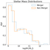 |
Fig. 1. Stellar mass distributions for the simulated TNG50 merger and non-merger galaxies used for fine-tuning Zoobot. There are 291 each of mergers and non-mergers, with 104 at z = 0.3. 111 at z = 0.2, and 76 at z = 0.1. Each merger galaxy used in the fine-tuning process has a corresponding non-merger galaxy at the same snapshot with a stellar mass within 0.1 dex. |
The sample used for fine-tuning includes 291 mergers and non-mergers of similar stellar mass distribution, and as each galaxy in the image catalog is processed by SKIRT along four lines of sight, we have ∼1200 synthetic HSC gri images each for mergers (assigned with a class label of 1) and non-mergers (assigned with a class label of 0). A sample size of this order can achieve greater accuracies through fine-tuning using Zoobot as opposed to training a model from scratch, or from transfer learning using ImageNet, as shown in Walmsley et al. (2022b). We note that while our merger sample includes mergers at varying mass ratios and stages, they are all given the same class label. As such, the output of our model will only predict whether or not a galaxy is a merger, and will not make classifications on merger mass ratio or stage.
Cutouts are made for the ∼2400 galaxy images as a final preprocessing step. These cutouts encompass 10× Sersic Reff of each galaxy, and are resized to 300 × 300 pixels for input into the model.
2.2.4. Training procedure
As highlighted in the previous sections, the “head” trained on GZ DeCALS is removed, and the “base” model is frozen. Detailed architecture of the Zoobot “base” model are available in Walmsley et al. (2022a). We summarize the newly added “head” layer for the merger identification task in Table 1.
Architecture of the new “head” model we attach to the Zoobot “base” model.
We train our new head using binary cross-entropy loss, with a maximum of 150 epochs available for training. However this maximum number of epochs may not necessarily be reached, as we follow Walmsley et al. (2022b) and adopt an early stopping algorithm, which ends training when the validation loss stops decreasing. The training time is dependant on the data-set size. For the small data-sets used in this work, each epoch takes about 50 s, with the longest training taking 48 epochs and the shortest 18 epochs.
Before we conduct tests on observational data, we first evaluate the performance of the model on simulation data alone. We split the TNG50 data-set into training, validation, and testing data-sets. To prevent contamination between the training and testing sample, we make sure that all four viewing angles of a single galaxy are contained in a single data-set. For example, if a galaxy with viewing angle 1 is included in the training data-set, the other three viewing angles are also included in the training data-set, and no angles of the same galaxy are in the testing or validation data-sets. We create ten independent training/validation/testing subsets through ten-fold cross validation so that each galaxy will be assigned a merger probability. The split for each data-set is 63% training, 27% validation, and 10% testing. We record the accuracy, loss, validation accuracy and validation loss of each run.
Table 2 reports the mean precision, recall, and f1-score for each class (merger and non-merger). A summary of the confusion matrices for each run are available in Appendix A. We note a stochasticity in validation accuracy and validation loss in the confusion matrices, likely resulting from the variation in the training/validation/testing data-set splits.
Means of metrics of ten individual Zoobot fine-tuning runs, assuming a complete binary class split (non-merger class (class 0): merger probability < 0.5, merger class (class 1): merger probability > 0.5).
The mean accuracy obtained from the ten runs is 76%. These results are comparable to or greater than previous works that trained CNNs from scratch using simulation images of galaxy mergers (e.g., Pearson et al. 2019a), with this work using a far smaller set of training data. For example, Pearson et al. (2019a) uses ∼7000 images to train their simulation network, and achieves an accuracy of 65.2%. We can expect a further increase in training data by incorporating mergers and non-mergers from more TNG snapshots when the images become available, which should further improve accuracies.
Making predictions on galaxies returns a merger probability between 0 and 1, with 0 indicating a non-merger galaxy and 1 indicating a merger galaxy, independent of merger mass ratio or merger stage. Figure 2 shows histograms of these probabilities for the 10 runs. In Fig. 2a we see that the probabilities are peaked in a range between 0.4–0.5, indicating that many galaxies have unclear classifications, and not as many galaxies are “confidently” labeled mergers or non-mergers. However, we find that more mergers are given a probability > 0.5, and more non-mergers are given a probability < 0.5. We further investigate what type of mergers are given unclear merger probabilities. Figure 2b shows the merger probability distributions on ground truth pre-merger (within 0.5 Gyr until the merger event) and post-merger (within 0.5 Gyr since the merger event) galaxy images. We find that while the model most frequently gives pre-mergers a probability > 0.8, post-mergers are found to be most frequently given a probability between 0.4–0.5. Figure 2c shows the merger probability distributions on ground truth major merger (mass ratio > 1:4), minor merger (1:4 > mass ratio > 1:10), and mini merger (1:10 > mass ratio > 1:20) images. We find that while the model is able to give high merger probabilities to mergers of all mass ratios, more minor and mini mergers are given lower probabilities (0.5 < merger probability < 0.8) compared to major mergers. As such, the galaxies given unclear merger probabilities are likely to be minor and mini post-mergers.
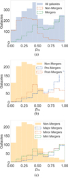 |
Fig. 2. Merger probability distributions for TNG50 synthetic galaxy images predicted using our fine-tuned model. We used ten-fold cross-validation during training for ten independent testing samples to find probabilities for all galaxies, so that each galaxy was given one probability during the process. Each subfigure shows the merger probability distributions for different types of ground-truth mergers. (a) All galaxies, mergers, and non-mergers. (b) Non-mergers, pre-mergers (0.5 Gyr > time until merger > 0 Gyr), and post-mergers (0.5 Gyr > time since merger > 0 Gyr). (c) Non-mergers, major mergers (mass ratio > 1:4), minor mergers (1:4 > mass ratio > 1:10), mini mergers (1:10 > mass ratio > 1:20). |
We next evaluated the model’s performance at various thresholds using an ROC curve. The ROC curve plots the true positive ( ) against the false positive (
 ) rates at all probability thresholds between 0 and 1. Figure 3 shows the ROC curve. The area under the ROC curve (AUC) measures the ability of the model, returning a value between 0 and 1. This value is the probability that a randomly selected merger has a merger probability greater than that of a randomly selected non-merger. An AUC of 1 indicates a perfect classifier. Our AUC is 0.84.
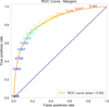 |
Fig. 3. Trained model’s ROC curve. The numbers overlayed on the curve indicate thresholds where the false positive and true positive rates along the curve are recorded. The dotted diagonal line is the performance of a completely random model that outputs a random probability for any image. An ROC curve is preferred to be above this dotted diagonal, and the curve generated from our model is above this line. We also find an AUC value of 0.84. |
We further show the model’s performance as a function of merger probability in Fig. 4a, in the form of mean completeness and precision curves of the 10 runs. The completeness is obtained by the dividing the number of ground truth mergers with a greater merger probability than the probability bin, by the total number of ground truth mergers in the testing data-set:
 (1)
(1)
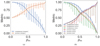 |
Fig. 4. Precision and completeness curves of the TNG images, with mean completeness and prevision as a function of merger probability. Left panel: curves assuming a complete binary split. The blue curve indicates completeness, and the orange curve indicates precision. Vertical error bars indicate the maximum and minimum values for the metric from the ten runs at each probability bin. Right panel: curves taking into consideration differing merger mass ratios (major, minor, mini). We find mini and minor mergers are predicted at an equivalent, if not greater precision compared to major mergers. We also find that the completeness at any fixed merger probability decreases with decreasing merger mass ratio. |
where GT means ground truth. The precision is obtained by the dividing the number of ground truth mergers with a greater merger probability than the probability bin by the total number of objects with a greater merger probability than the probability bin:
 (2)
(2)
The model has values of 80% for both completeness and precision for mergers on the testing data-set if we adopt a complete binary split, that is, any galaxy with a merger probability > 0.5 is classified as a merger, and any < 0.5 is classified as a non-merger. This accuracy can be considered a reasonable result (> 80%). However, if we adopt a merger and non-merger split based on “confident” predictions, or merger probability > 0.8, our mean accuracy increases to 91%.
We further investigated the role of the mass ratio in the completeness and precision curves. Figure 4b shows the mean precision and completeness as a function of the same merger probabilities; however, this time separating the major, minor, and mini mergers. We find that the mean precision at a binary split is 59% for major mergers, 63% for minor mergers, and 62% for mini mergers. These metrics increase to 80% for major mergers, 82% for minor mergers, and 79% for mini mergers for “confident” merger probabilities. The precision values are lower when the mergers are split by mass ratio as opposed to a two-class split due to the method of computing the metrics. There are an equal number of overall mergers and non-mergers; however, the respective numbers of major, minor, and mini mergers are lower than the number of non-mergers in each test data-set. As a result while the numerator in Eq. (2) accounts only for mergers of the labeled mass ratio, the denominator includes all non-mergers and mergers regardless of mass ratio. As such, our findings with respect to the precisions shown in Fig. 4b are more relevant in a qualitative manner rather than quantitative. Noting the gradients for the metric curves, we find that the completeness curve for major mergers drops off most gradually, indicating that our model is most confident in classifying major mergers. We also note that the precision for mini mergers (mass ratio < 1:20) is the highest between the three mass ratios at a binary split, and remains the highest at the “confident” probabilities, indicating that the model is able to predict mini mergers at an equivalent or greater precision compared to major and minor mergers. This precision will allow for studies using large, precise samples of sub-major mergers, which have adverse effects on galaxy properties such as size growth (Bédorf & Portegies Zwart 2013; Lang et al. 2014; Martin et al. 2018; Bottrell et al. 2023).
We provide some examples of true positive, true negative, false positive, and false negative galaxy classifications from the 10 runs in Figs. B.1–B.4, respectively, adopting a completely binary split. With this split, the model seems to be able to identify mergers of diverse morphologies, ranging from interacting pairs to merger remnants with visual signatures. We also find that the model is able to identify non-mergers of diverse morphologies, including projections, overlaps, and isolated galaxies, as shown in the varying appearances of true negative predictions in Fig. B.2. The model seems to have mixed results on galaxy projections, as there are examples in both Fig. B.3 (false positives) and Fig. B.2 (true negatives). For incorrectly classified mergers (false negatives), many of the mergers with low probabilities (merger probability < 0.3) are those with large mass ratios (μ < 0.25) whose times since or until the nearest merger event are close to the selection threshold of 0.5 Gyr (> 0.3 Gyr), meaning that potential merger indicators may not be visible, for example 84-569599_v0 (merger probability 0.05) in row 4, Col. 5 of Fig. B.4 is a mini merger that is 0.31 Gyr until its merger event, and look visually very similar to non-mergers. Many of these galaxies would also likely not be classified as mergers by human-based visual classification methods. However, we also note there are also misclassifications with major mergers, for example 84-577873_v0 (merger probability 0.40) in row 3, Col. 4 of Fig. B.4 is a major merger that is 0.49 Gyr until its merger event, which would likely be labeled as a merger by human-based methods. For misclassified non-mergers (false positives), galaxies with high merger probabilities (> 0.8) are likely to be classified as merging by human-based methods, as they show merger-like disturbances, and may also have projections. As such, our machine-learning based approach may encounter similar issues as previous human-based visual approaches. Nevertheless, even with its misclassifications, we find that the model is able to correctly classify a diverse range of mergers and non-mergers, which should be useful for merger galaxy sciences.
3. Predictions from observations
In this section, we describe the work we do to make predictions from observational images using the fine-tuned model. For the work conducted in this section, we trained a new head model using a 70% training and 30% validation split of the simulation data-set used in the previous section, and no further split of testing data, and attached it to the original Zoobot base model. Armed with our fine-tuned Zoobot model, we apply it to SDSS and GAMA spectroscopically confirmed galaxies in the HSC-SSP public data release 3 (Aihara et al. 2022). The training with this split lasted 37 epochs, with a duration of 23 min using GPU (NVIDIA Quadro P400).
The HSC-SSP is a multi-tiered, wide-field, multi-band imaging survey on the Subaru 8.2 m telescope on Maunakea in Hawaii. Detailed information about the survey, its instrumentation, and its techniques are available in Aihara et al. (2018) and relevant papers (Bosch et al. 2018; Miyazaki et al. 2018; Komiyama et al. 2018; Furusawa et al. 2018). We use data from HSC-SSP due to its wide field of observation and exceptional ground-based depth and resolution. In its widest component (Wide layer), HSC-SSP covers about 600 deg2 of the sky in five broad band filters (grizy), with observations from 330 nights coadded. The depth of the HSC survey is r ≈ 26 mag (5σ, point source) for the Wide layer. The coverage and depth of HSC-SSP will give us access to high quality imaging data of several million galaxies. We plan to make merger probabilities for all of HSC-SSP Wide in future works, a catalog of which will be made publicly available for the benefit of the galaxy astronomy community. This merger probability catalog is expected to be one of the largest catalogs of its kind.
For the work conducted in Sect. 5, we use a subsample of galaxies from the HSC-SSP Wide internal data release S21A catalog to conduct predictions on with our trained model. To select a galaxy sample, we cross-match HSC-SSP S21A galaxies to SDSS Data Release 17 (Abdurro’uf 2022) and Galaxy And Mass Assembly Data Release 4 (GAMA DR4, Driver et al. 2022) galaxies within 1 sky arcsec. We are left with 145 544 matches in SDSS and 156 604 matches in GAMA, for a total of 302 148 galaxies. All galaxies matched have spec-z measurements from their respective catalogs. We only use spectroscopic redshifts, due to photometric redshift errors. The galaxies have a magnitude limit of r < 17.7 mag for SDSS galaxies and r < 19.8 for GAMA galaxies. The galaxies lie within a redshift range of z = 0.01 − 0.35 and have M* = 3 × 10⁹ − 3 × 10¹¹ M⊙. M* values are obtained following Chen et al. (2012) for the SDSS galaxies and its own catalog for the GAMA galaxies. The SDSS galaxy stellar masses, using a principal component analysis method on SDSS spectra. First, a model spectra is created based on Bruzual & Charlot (2003) stellar population synthesis model. Next, principal components are identified from the model library. Finally, the SDSS spectra are fitted to the model and physical properties estimated. The masses obtained are consistent with the GALEX-SDSS-WISE Catalog (Salim et al. 2016, 2018). The GAMA galaxy stellar masses are obtained using the SED fitting code MAGPHYS (Driver et al. 2018). MAGPHYS also uses a library based on Bruzual & Charlot (2003). Sets of optical and infrared spectra are regressed toward flux measurements and errors to find a best-fit SED and physical parameters, including stellar mass.
Each galaxy in the catalog also has several environmental parameters related to its local mass density, studied in Yesuf (2022). The stellar mass overdensities within radii of 0.5, 1, and 8 h−1 Mpc, as well as within the radii determined by the projected distance to the fifth nearest neighbor are calculated. Only galaxies within |Δv|< 1000 km s−1 relative to the primary source are considered in this calculation. This cutoff prevents unrelated foreground or background galaxies from being included. The densities are normalized by the median densities of all galaxies within a given mass range and redshift bin, making them overdensities relative to the median in the redshift bin. Details on how the densities are calculated are written in Yesuf (2022) and the papers referenced within.
We make predictions on gri images for each HSC galaxy, with the images having the same dimensions as the synthetic HSC images of the TNG50 galaxies – cutouts encompassing 10 × Reff, re-sized to 300 × 300 pixels. For each input image, our model will output a merger probability between 0 and 1, with 0 indicating non-merger and 1 indicating a merger, again independent of merger mass ratio or merger stage.
We note that some HSC galaxy identifications are susceptible to “bright galaxy shredding,” discussed in Aihara et al. (2018). Bright (i < 19) galaxies, especially of late-type, are deblended into multiple objects, with the debelending seen even after cross-matching with a spectroscopic catalog. An inspection of the non-cropped image of objects affected by shredding reveals that that it is part of the spiral arm of a larger galaxy. As much as 15% of bright galaxies in HSC-SSP suffer from shredding, so it is expected that there are galaxies suffering from similar effects in our classified samples. However, these issues are expected to be resolved when making predictions on future HSC-SSP public data releases. For this work, as we are using the SDSS/GAMA coordinates and their petrosian radii to make our cutouts, we should not be as affected by shredding compared to HSC data.
4. Results
4.1. Prediction results
We plot a histogram of the merger probabilities of the SDSS and GAMA galaxies in Fig. 5. We see that the outputted probabilities are diverse in range, with the most galaxies being assigned “unconfident” labels, with the peak being between 0.1–0.5 for the SDSS galaxies and 0.3–0.5 for the GAMA galaxies. This location of the peak is similar to that found in the simulation predictions in the previous section, but differs from the probabilities found by transfer learning in Ackermann et al. (2018), Ferreira et al. (2020), where very clear probabilities both for mergers and non-mergers were favored. A possible explanation for the difference in distribution between our results and previous works, i.e., the peak in the 0.1–0.6 merger probability range, is the inclusion of the substantial number of mini mergers in our training sample. We will be able to examine this upon the completion of the images in Bottrell et al. (2023), as we will have many more major and minor mergers to fine-tune our model with. Many galaxies with similar appearances as the true mini mergers used in the fine-tuning process could be assigned “unconfident” merger probablities in this range, whether they be merging or non-merging in ground truth. However, we also note the secondary peak at higher merger probability (> 0.9), meaning many mergers are confidently identified. This is consistent with the above mentioned works, and also allows for a large “confident” merger sample for science purposes.
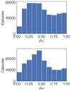 |
Fig. 5. Merger probability distributions for HSC-SDSS (upper) and HSC-GAMA (lower) cross-matched galaxies predicted using our fine-tuned model. Note that in both cases, more galaxies lie in an unclear range (merger probability 0.2 − 0.5) for non-mergers than “confident” non-mergers (merger probability 0 − 0.1). However, we find that many of the mergers identified are confident (merger probability > 0.8). |
We show examples of galaxies within various merger probability bins in our predicted samples in Figs. C.1–C.4. We find that in the low merger probability bins (merger probabilities 0 − 0.3, Fig. C.1), our model correctly identifies likely stellar overlaps and projections as non-mergers, as well as a diverse appearance of non-mergers, similar to the correctly identified non-mergers in the simulation data. On the high merger probability end (merger probabilities > 0.8), similar to as seen in the simulation data, the model can predict mergers with diverse appearances, including clear interacting pairs and late or early stage mergers with disturbances.
As further validation, we confirm our model’s ability to differentiate between projections and physically connected pairs in observational images. For each galaxy within our two samples that has a neighbor within a 30 kpc physical aperture, we calculate the line-of-sight velocity offset between the galaxy and its neighbor by Δv = cΔz/(1 + ztarget). We plot the merger probability distribution of these galaxies, binned by the line-of-sight velocity offset with its neighbor, or in the case of galaxies with multiple neighbors the minimum line-of-sight velocity offset, in Fig. 6. We find that pairs with offset Δv < 500 km s−1 makes up the greatest fraction of galaxies pairs with merger probability > 0.8, and as the velocity offset increases, a greater distribution of galaxies are given unclear to lower merger probabilities (merger probability < 0.5). Of the galaxies with both a high merger probability and offset, while a fraction of which may be projections, there are also likely to be true mergers that coincidentally have a projection. In particular, there may be post-merger galaxies that are not a pair but still have high merger probability. Based on our simulation results in Fig. 2b, our model identifies 1 post-merger galaxy for every 2 pre-merger galaxies. Following these results, a fraction of galaxies with Δv > 500 km s−1 and high merger probabilities in Fig. 6 are likely to be post-mergers.
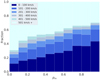 |
Fig. 6. Merger probability distributions for galaxies with a spectroscopically identified pair within a 30 kpc radius aperture, binned by velocity difference of the pair. The vertical axis represents the fraction of galaxies in each merger probability bin belonging to each velocity difference bin. We find that the fraction of smaller velocity difference galaxy pairs increases monotonically with merger probability bin. |
4.2. Merger sample selection for science
The results from simulation data show that a complete binary split, or in other words a merger probability > 0.5 is a merger and < 0.5 is a non-merger, gives a precision that is ∼80%. However, the merger probability distribution for both observation and simulation results show that many galaxies lie in a range between merger probability 0.2 − 0.6. As such, while the merger probabilities we found can be sufficiently useful to investigate trends between merger probability and physical properties, conducting studies adopting a complete binary split may suffer from contamination of “unconfident” galaxies. We can see from Fig. C.3 that there are many unclear galaxies in the probability range 0.5 − 0.8 that may or may not be real mergers; thus, using galaxies in this range may contaminate both merger and non-merger samples.
We plot the merger fraction of our two samples as a function of merger probability in Fig. 7. We compare our results with previous works calculating the merger fraction in similar redshift ranges, both in observations and simulations (Lotz et al. 2011; Cotini et al. 2013; Pearson et al. 2019b; Kim et al. 2021; Nevin et al. 2023). We find that our merger fractions, in most cases, become statistically consistent with these works if we consider “confident” classifications (merger probability > 0.8) as our threshold, with the threshold indicated by the dotted vertical line. However, we note that despite the statistical consistency there are likely to be contaminants regardless of threshold.
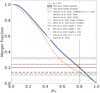 |
Fig. 7. Merger fraction as a function of merger probability for our two samples. The black vertical dotted line indicates the “confident” merger probability threshold of 0.8. We also plot the merger fractions found in Pearson et al. (2019b, red, green, and yellow lines), Nevin et al. (2023, brown lines), Kim et al. (2021, black lines), Lotz et al. (2011, light blue dotted line), and Cotini et al. (2013, purple line). We find that our merger fraction matches those of previous studies at increased merger probabilities. |
We will not set a definite, arbitrary threshold to define a merger in the catalog to be released; instead, we will just provide the merger probabilities for every galaxy, as shown in Table 3, and users can determine their thresholds. However, we recommend that a “confident” threshold (merger probability > 0.8) is used to determine a merger sample.
HSC merger probability catalog.
5. Merger galaxy properties
In this section, we use merger probabilities obtained using our model to investigate the relationship between galaxy mergers and local galaxy environments. We evaluate the merger probability distribution in differing environmental density bins for the various environmental parameters. We also investigate the relationship between galaxy merging and environment in TNG simulations, and look for any agreements between observations and simulations.
5.1. Environmental overdensities as a function of merger probability
Figure 8 shows the cumulative distributions of merger probability in bins of various environment metrics described in Sect. 3. The distributions are split into separate density bins, depending on the scale of the parameter used.
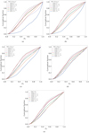 |
Fig. 8. Cumulative distribution curves of merger probabilities of HSC galaxies cross-matched with GAMA (dotted lines) and SDSS (solid lines) predicted by our fine-tuned model, for environmental densities at differing apertures. log(1 + δ5) Each curve represents a different environmental density bin. The gradients of these curves show that in lower density environments, there are more higher merger probability galaxies, and in higher density environments, there are more galaxies with lower merger probabilities. This trend holds true for each parameter investigated. The trend also holds qualitatively between the SDSS and GAMA samples. The environmental parameters are as follows, and we also indicate the KS test statistic between the densest and least dense regions in each figure as reference. Upper left panel: 0.1 h−1 Mpc stellar mass overdensity log(1 + δ0.1 h−1 Mpc), KS test (SDSS) statistic: 0.394, KS test (GAMA) statistic: 0.238. Upper right panel: 0.5 h−1 Mpc stellar mass overdensity log(1 + δ0.5 h−1 Mpc), KS test (SDSS) statistic: 0.417, KS test (GAMA) statistic: 0.184. Middle left panel: 1 h−1 Mpc stellar mass overdensity log(1 + δ1 h−1 Mpc), KS test (SDSS) statistic: 0.341, KS test (GAMA) statistic: 0.143. Middle right panel: 8 h−1 Mpc stellar mass overdensity log(1 + δ8 h−1 Mpc), KS test (SDSS) statistic: 0.183, KS test (GAMA) statistic: 0.127. Bottom panel: fifth nearest neighbor mass overdensity, KS test (SDSS) statistic: 0.191, KS test (GAMA) statistic: 0.069. |
The upper left panel of Fig. 8 shows the sensitivity of merger probability to environmental overdensities at 0.1 h−1 Mpc scales (0.2 h−1 Mpc aperture, centered on the target galaxy). The upper right panel shows the same at 0.5 h−1 Mpc scales (1 h−1 Mpc aperture). The middle left panel shows the same at 1 h−1 Mpc scales (2 h−1 Mpc aperture). The middle right panel shows the same at 8 h−1 Mpc scales (16 h−1 Mpc aperture). The bottom panel shows the sensitivity of merger probability to environmental overdensities within the radii of the target galaxy’s fifth nearest neighbor. From blue to red, the curves show the cumulative distributions of merger probability in increasingly dense environments.
We find a clear difference in the distribution curves and histograms between the lowest density (log(1 + δx) < − 1.0) and highest density (log(1 + δx) > 1.0) environments, with a similar trend holding across all five environmental parameters investigated. In each panel, we find that the lowest density environments contain the largest number of galaxies with high merger probability, as seen by the blue curve in each panel. This is the most pronounced in the blue curves in the upper left (0.5 h−1 Mpc) and upper right (1 h−1 Mpc) panels, but still qualitatively hold true in the bottom two panels (8 h−1 Mpc and fifth nearest neighbor scale). Conversely, we find that higher density environments contain the largest number of galaxies with low merger probability, as seen by the red curves.
In higher density environments (log(1 + δx) > 0.0), we find that galaxies with a lower merger probability tend to be in this environment, as seen by the red and green curves. For lower density environments (log(1 + δx) < 0.0), we find that the opposite holds true, that higher-merger-probability galaxies tend to be in lower density environments, shown by the blue and orange curves. We also find that these trends, in general, qualitatively hold true regardless of stellar mass of the target galaxy, as shown in Appendix D. In most figures, the most mass-overdense regions have more galaxies with low merger probability, and high-merger-probability galaxies are more likely to lie in mass-underdense regions. We note that the terms mass-overdense and -underdense do not necessarily refer to group members and non-group members, and we find no differences when investigating these qualitative trends separately for group and non-group members. Further, as the stellar mass overdensities have a strong correlation with halo mass (Yesuf 2022), these trends also appear at differing halo mass scales.
These results are consistent with the findings of works such as Ghigna et al. (1998), Lin et al. (2010) and Alonso et al. (2012). These works, with environments computed at similar scales, suggest that mergers and merging pairs are more likely to happen in less dense environments. In addition, spectroscopic pair matching methods with strict spectroscopic cuts are more likely to produce results similar to our findings (Ellison et al. 2010).
However, we also note that these results contradict with the suggestion that galaxy interactions are associated with intermediate to higher density regions, where galaxies have close companions and neighbors (Darg et al. 2010a; Jian et al. 2012). For example, Darg et al. (2010a) found that at the log(1 + δ2 h−1 Mpc) scale, even though both mergers and non-mergers peak in an intermediate environment, mergers occupy a slightly denser environment, which differs from our findings. We discuss possible reasons in Sect. 6.
5.2. Comparison with simulation data
Figures 9–15 show the cumulative histograms of environmental distributions of a total of 244 722 TNG50 and TNG100 mergers and non-mergers between snapshots 59 and 99 (redshifts 0.7 > z > 0.1), grouped by redshift, further split into two subfigures, with the left figure accounting for companions with mass ratio > 1:4 (major companions) and the right figure accounting for companions with mass ratio > 1:10 (major and minor companions), for each parameter. The mergers and non-mergers were selected using the same timescale criteria used in creating the fine-tuning data-set for Zoobot, for a total of 17 877 mergers and 226 895 non-mergers. The environmental parameters used – the stellar mass overdensities within a spherical volume with radii of 0.05, 0.1, 0.5, 1, 2, and 8 h−1 Mpc as well as within the radii of the fifth nearest neighbor – are similar to the observations and were calculated through computations similar to those used for the environmental parameters of the observations in Sect. 3. We also make the environmental distributions from the SDSS observations visible where the data are available: the density within the 0.1 h−1 Mpc, 0.5 h−1 Mpc, 1 h−1 Mpc, 8 h−1 Mpc radii spherical volume, and the radii of the fifth nearest neighbor. We split the observational data in four different merger probability bins, with pm < 0.3, 0.3 < pm < 0.5, 0.5 < pm < 0.8, and 0.8 < pm.
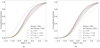 |
Fig. 9. Environment distribution cumulative histograms of the environmental densities within a spherical volume including the fifth nearest neighbor to the target galaxy, for TNG50 and TNG100 mergers and non-mergers. From left to right: (a) environmental mass densities taking into account companions with mass ratio > 1:4 (major companions), and (b) environmental mass densities taking into account companions with mass ratio > 1:10 (major and minor companions). We also make the histograms for the observational data visible as reference where available, indicated by the dotted lines. KS test statistics between simulation mergers and non-mergers, as well as between confident mergers (merger probability > 0.8) and non-mergers (merger probability < 0.3) are indicated. Major companions (left panel): KS test (Simulation) statistic: 0.226, KS test (Observation) statistic: 0.131. Major and minor companions (right panel): KS test (Simulation) statistic: 0.194, KS test (Observation) statistic: 0.131. |
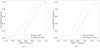 |
Fig. 10. Same as Fig. 9, but for stellar mass overdensities within a 50 kpc radii spherical volume. Major companions (left panel): KS test (Simulation) statistic: 0.348. Major and minor companions (right panel): KS test (Simulation) statistic: 0.353. |
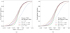 |
Fig. 11. Same as Fig. 9, but for stellar mass overdensities within a 100 kpc radii spherical volume. Observational data are available for this parameter. Major companions (left panel): KS test (Simulation) statistic: 0.285, KS test (Observation) statistic: 0.231. Major and minor companions (right panel): KS test (Simulation) statistic: 0.260, KS test (Observation) statistic: 0.231. |
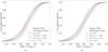 |
Fig. 12. Same as Fig. 9, but for stellar mass overdensities within a 500 kpc radii spherical volume. Observational data are available for this parameter. Major companions (left panel): KS test (Simulation) statistic: 0.108, KS test (Observation) statistic: 0.171. Major and minor companions (right panel): KS test (Simulation) statistic: 0.100, KS test (Observation) statistic: 0.171. |
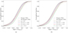 |
Fig. 13. Same as Fig. 9, but for stellar mass overdensities within a 1 Mpc radii spherical volume. Observational data are available for this parameter. Major companions (left panel): KS test (Simulation) statistic: 0.140, KS test (Observation) statistic: 0.168. Major and minor companions (right panel): KS test (Simulation) statistic: 0.129, KS test (Observation) statistic: 0.168. |
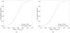 |
Fig. 14. Same as Fig. 9, but for stellar mass overdensities within a 2 Mpc radii spherical volume. Major companions (left panel): KS test (Simulation) statistic: 0.147. Major and minor companions (right panel): KS test (Simulation) statistic: 0.131. |
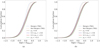 |
Fig. 15. Same as Fig. 9, but for stellar mass overdensities within a 8 Mpc radii spherical volume. Observational data are available for this parameter. Major companions (left panel): KS test (Simulation) statistic: 0.153, KS test (Observation) statistic: 0.102. Major and minor companions (right panel): KS test (Simulation) statistic: 0.123, KS test (Observation) statistic: 0.102. |
We find two differing trends in the simulational data, depending on the scale of the environmental density parameter. For the environmental density parameters of the scale of 0.5 h−1 Mpc and larger, and for fifth nearest neighbor environments, a greater fraction of mergers lie in mass-underdense environments, and a greater fraction of non-mergers lie in mass-overdense environments, indicating a similar trend as that seen with the predictions from observational data, as the fraction of mergers in lower density environments increases with increasing merger probability bin. We also find that there are very little to no mergers found in the densest environments for each of these parameters. We also find that these trends are, in general, not sensitive to mass ratio, and hold true for all investigated redshift bins up to z = 0.7. As such, we have a consistency in the relationship between galaxy mergers and environmental densities between observations and simulations at equivalent scales.
Conversely, we find that the above trend is reversed for the environmental density parameters within the spherical volume of 0.05 and 0.1 h−1 Mpc, found in Figs. 10 and 11, respectively. That is, at these scales, we find that the majority of non-mergers are in the lowest density environments, as shown by the brown, red, and orange lines, and mergers are found in denser environments, as shown by the blue, green, and purple lines. These trends are also not sensitive to mass ratio or redshift. However, this reversal does not occur in the observational data, as shown in Fig. 11. While the behavior of the low merger environment curves show a steeper gradient in underdense regions (0.5 < log(1 + δx) < 0.0), the trend is qualitatively similar as the larger scales. Further investigation is required on the inconsistency between the observations and simulations at this scale, particularly as they are consistent at larger scales. We plan to investigate this in future works.
6. Discussion
Based on our merger probabilities and subsequent analysis in the previous section, our investigation finds that at the scales of 0.5 h−1 Mpc and greater, or close to the cluster scale and larger, merger galaxies are more prevalent in lower density environments, and higher density environments have a lower merger incidence, with this trend found both in observations and simulations. At the 0.1 h−1 Mpc and lower scales, or close to the galaxy scale, there are more non-mergers in lower density environments in the simulations; however, this reversal does not occur in our observational data.
Previous studies that have investigated the environmental dependence of merger activity have found varying results, with some works finding a greater merger fraction in higher density environments (Jian et al. 2012), and others finding merger fraction peaks in intermediate environments (Perez et al. 2009), and others finding that mergers are more likely to occur in lower density environments (Ghigna et al. 1998). We have results showing that the merger prevalence can be increased at both high and low density environments, with the trend differing depending on the scale of the environmental parameter.
In the richest environments, such as in the center of clusters, velocity dispersions are high, at scales of ∼1000 km s−1 (Struble & Rood 1999). At these speeds, galaxy-galaxy interactions are likely to be elastic encounters, and mergers and infall are less likely to occur (Kuntschner et al. 2002). Such encounters can strip the gas required to fuel star formation events (Gunn et al. 1972), and hence be a catalyst for dynamical evolution in cluster galaxies, but the final product of the interaction will likely not be a merger, resulting in lower merger incidence. As such, while higher density regions can have an increased pair fraction, but a lowered merger fraction (Lin et al. 2010). Conversely, in lower density environments, accretion and merger events can occur more frequently.
At a smaller scale, such as in the galaxy scale, over 90% of non-merger galaxies are found in lower density environments, and higher density environments are mostly populated with mergers. At this scale, galaxies are likely to be at closer projected separation with its neighbors compared to at greater scales, and hence be part of a merger. As a result, higher densities at this scale means there is a greater likelihood of a neighbor being a physically connected merger, resulting in the reversal of the trend from the larger scales.
We suggest a possible reason for any disagreements with previous works, particularly in higher density environments, to be attributed to the difference in merger sample selection techniques. For example, Darg et al. (2010a), a work based on visual identification of mergers, finds that while both mergers and non-mergers peak in intermediate density environments, mergers occupy slightly denser environments than non-mergers. However, Ellison et al. (2010), a work using spectroscopic pair selection, finds that a significant fraction of galaxy pairs are in higher density environments, but they also suggest that lower density environments are where mergers are likely to occur, a suggestion that is consistent with our results.
Different merger sample selection methods will lead to different merger samples, some with very little overlap (De Propris et al. 2007), and as such, trends in physical properties such as environment may differ. Additionally, some methods may be susceptible to overestimation of merger galaxies and contamination.
Spectroscopic pair matching methods can contaminate merger samples with interlopers. In high velocity dispersion environments, using the line-of-sight velocities as a proxy for three-dimensional velocities has limitations, and is strongly affected by interlopers (Saro et al. 2013), and galaxies may be considered merging pairs even if they are not physically connected. As such, merger catalogs created using these methods can overestimate the merger fraction.
Similarly, image-based classification techniques can also be contaminated with stellar and galactic chance projections, in both visual identification (Darg et al. 2010a,b; Pearson et al. 2019a) and quantitative morphologies (De Propris et al. 2007). In visual identification, the lack of complete information for objects could lead to projected galaxy pairs and galaxy-star pairs to be incorrectly classified as mergers. Such projections and galaxy-star pairs can also pose difficulties when conducting studies with quantitative morphologies such as asymmetries. The source extraction algorithms used may incorrectly deblend galaxy images containing projections, leading to highly asymmetric non-mergers. Contaminations from projections are likely to be more frequent in higher density environments.
Moreover, we note that our environment parameters discriminate by mass-overdense and -underdense regions, with no specification on group or cluster membership. While number-overdense environments, such as groups and clusters, do have evidence of merger activity, particularly at z > 1 (Lemaux et al. 2012; Tomczak et al. 2017; Liu et al. 2023), our parameters focus on the masses of these environments. In mass-overdense environments, as our figures do show, there are still galaxies with high merger probabilities to be found. These galaxies are likely dry merger systems occurring in groups or cluster environments, particularly important for the formation of early-type brightest cluster galaxies (BCGs) in cluster centers (Mulchaey et al. 2006; Rines et al. 2007; McIntosh et al. 2008; Tran et al. 2008; Liu et al. 2009; Lin et al. 2010; Burke & Collins 2013; Lidman et al. 2013; Ascaso et al. 2014). However, at redshift z < 1, many BCGs have finished their growth, and while there are BCGs that continue their growth through mergers at these redshifts, such cases are a minority (Collins et al. 2009; Stott et al. 2010, 2011; Liu et al. 2015; Runge & Yan 2018). Further, in the most mass-overdense environments, at z < 1, merger activity is suppressed due to increased velocity dispersions (Pipino et al. 2014), leading to a lower merger fraction in these environments. In mass-underdense environments, such as in field environments, or the outskirts of clusters and groups, the likelihood of finding a merger increases (Ghigna et al. 1998; Oh et al. 2019). This is also found at higher redshifts, both in the field (Delahaye et al. 2017) and in outskirt (Koulouridis & Bartalucci 2019) regions. As such, the fraction of mergers in mass-underdense regions should be greater than that in mass-overdense regions, which is consistent with our results.
Our environmental trends, particularly the decreased fraction of mergers in higher density environments, show that our morphology-based classification model is likely able to differentiate and give low merger probabilities to images of interlopers, or in other words non-merging pairs in higher density environments, an issue that needs corrections in both spectroscopy-based and image-based classification methods. We note that our environmental trends on observational data may harbor an implicit bias due to the morphology-density relation (Dressler 1980). The high velocity encounters in higher density environments can strip gas in galaxies, leading to visual morphologies exhibiting more smoother, spheroidal features. As such, galaxies in higher density environments are less likely to exhibit the tidal features that are present in mergers, resulting in such galaxies to be assigned low merger probabilities by our morphology-based merger identification model. However, we suggest that such a bias can be mitigated. First, the findings in Darg et al. (2010a), based on visual classification, suggest that mergers are more likely found in higher density environments, which contradicts what is found in comsmological n-body and hydrodynamical simulations. As the implicit biases due to the morphology density relation can be overlooked by visual classification studies, we suggest that a similar overlook is possible in our work. Second, the ground truth merger selection in our fine-tuning process is based on the time to the closest merger event, and is not be biased to any environments and morphlogies.
Investigations on the physical properties of the merger galaxies, such as projected separation and relative velocity differences with their neighbors, as well as colors, star formation rates and morphologies, are planned in future works, to determine if there are any environmental dependences on the properties of the mergers themselves in addition to merger incidence.
7. Conclusion
In this work, we take a deep learning based approach for merger classification in Subaru HSC-SSP. We fine-tune the pretrained model Zoobot using synthetic HSC images of galaxies in the Illustris TNG simulations, then make predictions using the fine-tuned model on a sample of galaxies in HSC-SSP S21A wide cross-matched with SDSS and GAMA. We find that the fine-tuning approach can achieve accuracies comparable to previous merger classification studies using simulational data, at a 76% accuracy, as well as 80% completion and precision. We achieved these results requiring a far smaller sample size than previous studies, sufficing with ∼103 training samples of each class. We also find that our morphology-based model is able to correctly predict both mergers and non-mergers of diverse appearances, mergers of differing mass ratios and stages, and can also distinguish to a degree between projections and true merging pairs. The merger rate found by our model is consistent with those of previous works if we adopt a “confident” threshold.
We have made the merger catalog we produced in this work publicly available. We plan to classify all of HSC-SSP in the future and make the results publicly available as well.
Further, we studied the relationship between merger activity and multi-scale galaxy environments in both the simulation data of TNG and the observational data of HSC-SSP, and compared our results. We find two trends in the simulation data, and one trend in the observational data. Both sets of data are in agreement that at scales of 0.5 h−1 Mpc and larger, merger galaxies favor lower density environments, and non-mergers favor higher density environments. However, below these scales, the simulation data finds that non-merger galaxies are most prevalent in lower density environments, and higher density environments favor mergers. In future works, we plan to investigate in both observations and simulations where the reversal in trend occurs, as well as the galaxy properties of the mergers themselves.
Acknowledgments
We would first and foremost like to thank the native Hawaiians for sharing the Maunakea mountain, a place of cultural, historical, and natural significance, allowing us access to a beautiful view of the Universe. Next, we would like to thank the anonymous referee for their comments and feedback in greatly improving the quality of this work. The Hyper Suprime-Cam (HSC) collaboration includes the astronomical communities of Japan and Taiwan, and Princeton University. The HSC instrumentation and software were developed by the National Astronomical Observatory of Japan (NAOJ), the Kavli Institute for the Physics and Mathematics of the Universe (Kavli IPMU), the University of Tokyo, the High Energy Accelerator Research Organization (KEK), the Academia Sinica Institute for Astronomy and Astrophysics in Taiwan (ASIAA), and Princeton University. Funding was contributed by the FIRST program from the Japanese Cabinet Office, the Ministry of Education, Culture, Sports, Science and Technology (MEXT), the Japan Society for the Promotion of Science (JSPS), Japan Science and Technology Agency (JST), the Toray Science Foundation, NAOJ, Kavli IPMU, KEK, ASIAA, and Princeton University. This paper is based [in part] on data collected at the Subaru Telescope and retrieved from the HSC data archive system, which is operated by Subaru Telescope and Astronomy Data Center (ADC) at NAOJ. Data analysis was in part carried out with the cooperation of Center for Computational Astrophysics (CfCA) at NAOJ. We are honored and grateful for the opportunity of observing the Universe from Maunakea, which has the cultural, historical and natural significance in Hawaii. This paper makes use of software developed for Vera C. Rubin Observatory. We thank the Rubin Observatory for making their code available as free software at http://pipelines.lsst.io/. The Pan-STARRS1 Surveys (PS1) and the PS1 public science archive have been made possible through contributions by the Institute for Astronomy, the University of Hawaii, the Pan-STARRS Project Office, the Max Planck Society and its participating institutes, the Max Planck Institute for Astronomy, Heidelberg, and the Max Planck Institute for Extraterrestrial Physics, Garching, The Johns Hopkins University, Durham University, the University of Edinburgh, the Queen’s University Belfast, the Harvard-Smithsonian Center for Astrophysics, the Las Cumbres Observatory Global Telescope Network Incorporated, the National Central University of Taiwan, the Space Telescope Science Institute, the National Aeronautics and Space Administration under grant No. NNX08AR22G issued through the Planetary Science Division of the NASA Science Mission Directorate, the National Science Foundation grant No. AST-1238877, the University of Maryland, Eotvos Lorand University (ELTE), the Los Alamos National Laboratory, and the Gordon and Betty Moore Foundation. This work has been supported by the Japan Society for the Promotion of Science (JSPS) Grants-in-Aid for Scientific Research (21H01128). This work has also been supported in part by the Collaboration Funding of the Institute of Statistical Mathematics “New Perspective of the Cosmology Pioneered by the Fusion of Data Science and Physics”. K.O. is supported by JSPS KAKENHI Grant Number JP23KJ1089. H.Y. was supported by JSPS KAKENHI Grant Number JP22K14072 and the Research Fund for International Young Scientists of NSFC (11950410492).
References
- Abdurro’uf, Accetta K., Aerts, C., et al. 2022, ApJS, 259, 35 [NASA ADS] [CrossRef] [Google Scholar]
- Ackermann, S., Schawinski, K., Zhang, C., Weigel, A. K., & Turp, M. D. 2018, MNRAS, 479, 415 [NASA ADS] [CrossRef] [Google Scholar]
- Aihara, H., Armstrong, R., Bickerton, S., et al. 2018, PASJ, 70, S8 [NASA ADS] [Google Scholar]
- Aihara, H., AlSayyad, Y., Ando, M., et al. 2022, PASJ, 74, 247 [NASA ADS] [CrossRef] [Google Scholar]
- Alonso, S., Mesa, V., Padilla, N., & Lambas, D. G. 2012, A&A, 539, A46 [NASA ADS] [CrossRef] [EDP Sciences] [Google Scholar]
- Ascaso, B., Lemaux, B. C., Lubin, L. M., et al. 2014, MNRAS, 442, 589 [NASA ADS] [CrossRef] [Google Scholar]
- Banerji, M., Lahav, O., Lintott, C. J., et al. 2010, MNRAS, 406, 342 [Google Scholar]
- Barnes, J. E., & Hernquist, L. 1992, ARA&A, 30, 705 [Google Scholar]
- Beckman, J., Carretero, C., & Vazdekis, A. 2008, Chin. J. Astron. Astrophys. Suppl., 8, 77 [Google Scholar]
- Bédorf, J., & Portegies Zwart, S. 2013, MNRAS, 431, 767 [CrossRef] [Google Scholar]
- Berg, T. A. M., Simard, L., Mendel, T. J., & Ellison, S. L. 2014, MNRAS, 440, L66 [NASA ADS] [CrossRef] [Google Scholar]
- Bershady, M. A., Jangren, A., & Conselice, C. J. 2000, AJ, 119, 2645 [NASA ADS] [CrossRef] [Google Scholar]
- Bickley, R. W., Bottrell, C., Hani, M. H., et al. 2021, MNRAS, 504, 372 [NASA ADS] [CrossRef] [Google Scholar]
- Bickley, R. W., Ellison, S. L., Patton, D. R., et al. 2022, MNRAS, 514, 3294 [NASA ADS] [CrossRef] [Google Scholar]
- Blumenthal, K. A., & Barnes, J. E. 2018, MNRAS, 479, 3952 [Google Scholar]
- Blumenthal, K. A., Moreno, J., Barnes, J. E., et al. 2020, MNRAS, 492, 2075 [CrossRef] [Google Scholar]
- Bosch, J., Armstrong, R., Bickerton, S., et al. 2018, PASJ, 70, S5 [Google Scholar]
- Bottrell, C., Simard, L., Mendel, J. T., & Ellison, S. L. 2019a, MNRAS, 486, 390 [NASA ADS] [CrossRef] [Google Scholar]
- Bottrell, C., Hani, M. H., Teimoorinia, H., et al. 2019b, MNRAS, 490, 5390 [NASA ADS] [CrossRef] [Google Scholar]
- Bottrell, C., Hani, M. H., Teimoorinia, H., Patton, D. R., & Ellison, S. L. 2022, MNRAS, 511, 100 [CrossRef] [Google Scholar]
- Bottrell, C., Yesuf, H. M., Popping, G., et al. 2023, MNRAS, in press, https://doi.org/10.1093/mnras/stad2971 [Google Scholar]
- Bruzual, G., & Charlot, S. 2003, MNRAS, 344, 1000 [NASA ADS] [CrossRef] [Google Scholar]
- Burke, C., & Collins, C. A. 2013, MNRAS, 434, 2856 [NASA ADS] [CrossRef] [Google Scholar]
- Burkey, J. M., Keel, W. C., Windhorst, R. A., & Franklin, B. E. 1994, ApJ, 429, L13 [NASA ADS] [CrossRef] [Google Scholar]
- Camps, P., & Baes, M. 2020, Astron. Comput., 31, 100381 [NASA ADS] [CrossRef] [Google Scholar]
- Carlberg, R. G., Pritchet, C. J., & Infante, L. 1994, ApJ, 435, 540 [NASA ADS] [CrossRef] [Google Scholar]
- Cavanagh, M. K., Bekki, K., & Groves, B. A. 2023, MNRAS, 520, 5885 [CrossRef] [Google Scholar]
- Chabrier, G. 2003, PASP, 115, 763 [Google Scholar]
- Chen, Y.-M., Kauffmann, G., Tremonti, C. A., et al. 2012, MNRAS, 421, 314 [NASA ADS] [Google Scholar]
- Cheng, T.-Y., Conselice, C. J., Aragón-Salamanca, A., et al. 2021, MNRAS, 507, 4425 [NASA ADS] [CrossRef] [Google Scholar]
- Ćiprijanović, A., Snyder, G. F., Nord, B., & Peek, J. E. G. 2020, Astron. Comput., 32, 100390 [CrossRef] [Google Scholar]
- Ćiprijanović, A., Kafkes, D., Downey, K., et al. 2021, MNRAS, 506, 677 [CrossRef] [Google Scholar]
- Collins, C. A., Stott, J. P., Hilton, M., et al. 2009, Nature, 458, 603 [Google Scholar]
- Conselice, C. J. 2003, ApJS, 147, 1 [NASA ADS] [CrossRef] [Google Scholar]
- Conselice, C. J., Bershady, M. A., & Jangren, A. 2000, ApJ, 529, 886 [NASA ADS] [CrossRef] [Google Scholar]
- Cotini, S., Ripamonti, E., Caccianiga, A., et al. 2013, MNRAS, 431, 2661 [NASA ADS] [CrossRef] [Google Scholar]
- Darg, D. W., Kaviraj, S., Lintott, C. J., et al. 2010a, MNRAS, 401, 1552 [NASA ADS] [CrossRef] [Google Scholar]
- Darg, D. W., Kaviraj, S., Lintott, C. J., et al. 2010b, MNRAS, 401, 1043 [NASA ADS] [CrossRef] [Google Scholar]
- Delahaye, A. G., Webb, T. M. A., Nantais, J., et al. 2017, ApJ, 843, 126 [NASA ADS] [CrossRef] [Google Scholar]
- De Propris, R., Conselice, C. J., Liske, J., et al. 2007, ApJ, 666, 212 [NASA ADS] [CrossRef] [Google Scholar]
- Dey, A., Schlegel, D. J., Lang, D., et al. 2019, AJ, 157, 168 [Google Scholar]
- Dieleman, S., Willett, K. W., & Dambre, J. 2015, MNRAS, 450, 1441 [NASA ADS] [CrossRef] [Google Scholar]
- Domínguez Sánchez, H., Huertas-Company, M., Bernardi, M., Tuccillo, D., & Fischer, J. L. 2018, MNRAS, 476, 3661 [Google Scholar]
- Domínguez Sánchez, H., Huertas-Company, M., Bernardi, M., et al. 2019, MNRAS, 484, 93 [Google Scholar]
- Domínguez Sánchez, H., Margalef, B., Bernardi, M., & Huertas-Company, M. 2022, MNRAS, 509, 4024 [Google Scholar]
- Dressler, A. 1980, ApJ, 236, 351 [Google Scholar]
- Driver, S. P., Andrews, S. K., da Cunha, E., et al. 2018, MNRAS, 475, 2891 [Google Scholar]
- Driver, S. P., Bellstedt, S., Robotham, A. S. G., et al. 2022, MNRAS, 513, 439 [NASA ADS] [CrossRef] [Google Scholar]
- Ellison, S. L., Patton, D. R., Simard, L., & McConnachie, A. W. 2008, AJ, 135, 1877 [NASA ADS] [CrossRef] [Google Scholar]
- Ellison, S. L., Patton, D. R., Simard, L., et al. 2010, MNRAS, 407, 1514 [NASA ADS] [CrossRef] [Google Scholar]
- Ellison, S. L., Patton, D. R., Mendel, J. T., & Scudder, J. M. 2011, MNRAS, 418, 2043 [NASA ADS] [CrossRef] [Google Scholar]
- Ellison, S. L., Patton, D. R., & Hickox, R. C. 2015, MNRAS, 451, L35 [NASA ADS] [CrossRef] [Google Scholar]
- Ellison, S. L., Viswanathan, A., Patton, D. R., et al. 2019, MNRAS, 487, 2491 [NASA ADS] [CrossRef] [Google Scholar]
- Fakhouri, O., & Ma, C.-P. 2009, MNRAS, 394, 1825 [NASA ADS] [CrossRef] [Google Scholar]
- Ferreira, L., Conselice, C. J., Duncan, K., et al. 2020, ApJ, 895, 115 [NASA ADS] [CrossRef] [Google Scholar]
- Ferreira, L., Conselice, C. J., Kuchner, U., & Tohill, C.-B. 2022, ApJ, 931, 34 [CrossRef] [Google Scholar]
- Furusawa, H., Koike, M., Takata, T., et al. 2018, PASJ, 70, S3 [Google Scholar]
- Ghigna, S., Moore, B., Governato, F., et al. 1998, MNRAS, 300, 146 [NASA ADS] [CrossRef] [Google Scholar]
- Ghosh, A., Urry, C. M., Wang, Z., et al. 2020, ApJ, 895, 112 [NASA ADS] [CrossRef] [Google Scholar]
- Goulding, A. D., Greene, J. E., Bezanson, R., et al. 2018, PASJ, 70, S37 [NASA ADS] [CrossRef] [Google Scholar]
- Groves, B., Dopita, M. A., Sutherland, R. S., et al. 2008, ApJS, 176, 438 [NASA ADS] [CrossRef] [Google Scholar]
- Gunn, J. E., Gott, J., & Richard, I. 1972, ApJ, 176, 1 [Google Scholar]
- Guzmán-Ortega, A., Rodriguez-Gomez, V., Snyder, G. F., Chamberlain, K., & Hernquist, L. 2023, MNRAS, 519, 4920 [CrossRef] [Google Scholar]
- He, K., Zhang, X., Ren, S., & Sun, J. 2015, 2015 IEEE International Conference on Computer Vision (ICCV) (IEEE), 1026 [CrossRef] [Google Scholar]
- Hernquist, L. 1989, Nature, 340, 687 [Google Scholar]
- Hernquist, L. 1992, ApJ, 400, 460 [NASA ADS] [CrossRef] [Google Scholar]
- Hester, J. A., & Tasitsiomi, A. 2010, ApJ, 715, 342 [NASA ADS] [CrossRef] [Google Scholar]
- Holincheck, A. J., Wallin, J. F., Borne, K., et al. 2016, MNRAS, 459, 720 [NASA ADS] [CrossRef] [Google Scholar]
- Hopkins, P. F., & Quataert, E. 2010, MNRAS, 407, 1529 [Google Scholar]
- Hopkins, P. F., Cox, T. J., Kereš, D., & Hernquist, L. 2008, ApJS, 175, 390 [Google Scholar]
- Hopkins, P. F., Cox, T. J., Hernquist, L., et al. 2013, MNRAS, 430, 1901 [Google Scholar]
- Huertas-Company, M., & Lanusse, F. 2023, PASA, 40, e001 [NASA ADS] [CrossRef] [Google Scholar]
- Jacobs, C., Collett, T., Glazebrook, K., et al. 2019, MNRAS, 484, 5330 [NASA ADS] [CrossRef] [Google Scholar]
- Jian, H.-Y., Lin, L., & Chiueh, T. 2012, ApJ, 754, 26 [NASA ADS] [CrossRef] [Google Scholar]
- Kawanomoto, S., Uraguchi, F., Komiyama, Y., et al. 2018, PASJ, 70, 66 [Google Scholar]
- Keel, W. C., Kennicutt, R. C. Jr., Hummel, E., & van der Hulst, J. M. 1985, AJ, 90, 708 [NASA ADS] [CrossRef] [Google Scholar]
- Kim, E., Hwang, H. S., Jeong, W.-S., et al. 2021, MNRAS, 507, 3113 [NASA ADS] [CrossRef] [Google Scholar]
- Kitzbichler, M. G., & White, S. D. M. 2008, MNRAS, 391, 1489 [NASA ADS] [CrossRef] [Google Scholar]
- Komiyama, Y., Obuchi, Y., Nakaya, H., et al. 2018, PASJ, 70, S2 [Google Scholar]
- Koss, M., Mushotzky, R., Veilleux, S., & Winter, L. 2010, ApJ, 716, L125 [Google Scholar]
- Koulouridis, E., & Bartalucci, I. 2019, A&A, 623, L10 [EDP Sciences] [Google Scholar]
- Krizhevsky, A., Sutskever, I., & Hinton, G. E. 2017, Commun. ACM, 60, 84 [CrossRef] [Google Scholar]
- Kuntschner, H., Smith, R. J., Colless, M., et al. 2002, MNRAS, 337, 172 [NASA ADS] [CrossRef] [Google Scholar]
- Lang, M., Holley-Bockelmann, K., & Sinha, M. 2014, ApJ, 790, L33 [Google Scholar]
- Lemaux, B. C., Gal, R. R., Lubin, L. M., et al. 2012, ApJ, 745, 106 [Google Scholar]
- Lidman, C., Iacobuta, G., Bauer, A. E., et al. 2013, MNRAS, 433, 825 [NASA ADS] [CrossRef] [Google Scholar]
- Lin, L., Koo, D. C., Willmer, C. N. A., et al. 2004, ApJ, 617, L9 [NASA ADS] [CrossRef] [Google Scholar]
- Lin, L., Cooper, M. C., Jian, H.-Y., et al. 2010, ApJ, 718, 1158 [NASA ADS] [CrossRef] [Google Scholar]
- Lintott, C. J., Schawinski, K., Slosar, A., et al. 2008, MNRAS, 389, 1179 [NASA ADS] [CrossRef] [Google Scholar]
- Lintott, C., Schawinski, K., Bamford, S., et al. 2011, MNRAS, 410, 166 [Google Scholar]
- Liu, F. S., Mao, S., Deng, Z. G., Xia, X. Y., & Wen, Z. L. 2009, MNRAS, 396, 2003 [NASA ADS] [CrossRef] [Google Scholar]
- Liu, F. S., Lei, F. J., Meng, X. M., & Jiang, D. F. 2015, MNRAS, 447, 1491 [NASA ADS] [CrossRef] [Google Scholar]
- Liu, S., Zheng, X. Z., Shi, D. D., et al. 2023, MNRAS, 523, 2422 [CrossRef] [Google Scholar]
- Lotz, J. M., Primack, J., & Madau, P. 2004, AJ, 128, 163 [NASA ADS] [CrossRef] [Google Scholar]
- Lotz, J. M., Jonsson, P., Cox, T. J., & Primack, J. R. 2008, MNRAS, 391, 1137 [Google Scholar]
- Lotz, J. M., Jonsson, P., Cox, T. J., & Primack, J. R. 2010a, MNRAS, 404, 590 [NASA ADS] [CrossRef] [Google Scholar]
- Lotz, J. M., Jonsson, P., Cox, T. J., & Primack, J. R. 2010b, MNRAS, 404, 575 [Google Scholar]
- Lotz, J. M., Jonsson, P., Cox, T. J., et al. 2011, ApJ, 742, 103 [Google Scholar]
- Marinacci, F., Vogelsberger, M., Pakmor, R., et al. 2018, MNRAS, 480, 5113 [NASA ADS] [Google Scholar]
- Martin, G., Kaviraj, S., Devriendt, J. E. G., Dubois, Y., & Pichon, C. 2018, MNRAS, 480, 2266 [Google Scholar]
- Matteo, T. D., Springel, V., & Hernquist, L. 2005, Nature, 433, 604 [NASA ADS] [CrossRef] [Google Scholar]
- McIntosh, D. H., Guo, Y., Hertzberg, J., et al. 2008, MNRAS, 388, 1537 [NASA ADS] [CrossRef] [Google Scholar]
- Mihos, J. C., & Hernquist, L. 1996, ApJ, 464, 641 [Google Scholar]
- Miyazaki, S., Komiyama, Y., Kawanomoto, S., et al. 2018, PASJ, 70, S1 [NASA ADS] [Google Scholar]
- Montuori, M., Di Matteo, P., Lehnert, M. D., Combes, F., & Semelin, B. 2010, A&A, 518, A56 [NASA ADS] [CrossRef] [EDP Sciences] [Google Scholar]
- Moreno, J., Torrey, P., Ellison, S. L., et al. 2015, MNRAS, 448, 1107 [NASA ADS] [CrossRef] [Google Scholar]
- Mulchaey, J. S., Lubin, L. M., Fassnacht, C., Rosati, P., & Jeltema, T. E. 2006, ApJ, 646, 133 [NASA ADS] [CrossRef] [Google Scholar]
- Naab, T., & Burkert, A. 2001, ASP Conf. Ser., 249, 735 [Google Scholar]
- Naab, T., & Burkert, A. 2003, ApJ, 597, 893 [Google Scholar]
- Naiman, J. P., Pillepich, A., Springel, V., et al. 2018, MNRAS, 477, 1206 [Google Scholar]
- Nair, P. B., & Abraham, R. G. 2010, VizieR Online Data Catalog: J/ApJS/186/427 [Google Scholar]
- Negroponte, J., & White, S. D. M. 1983, MNRAS, 205, 1009 [Google Scholar]
- Nelson, D., Pillepich, A., Springel, V., et al. 2018, MNRAS, 475, 624 [Google Scholar]
- Nelson, D., Pillepich, A., Springel, V., et al. 2019, MNRAS, 490, 3234 [Google Scholar]
- Nevin, R., Blecha, L., Comerford, J., et al. 2023, MNRAS, 522, 1 [NASA ADS] [CrossRef] [Google Scholar]
- Oh, S., Kim, K., Lee, J. H., et al. 2019, MNRAS, 488, 4169 [CrossRef] [Google Scholar]
- Patton, D. R., Pritchet, C. J., Yee, H. K. C., Ellingson, E., & Carlberg, R. G. 1997, ApJ, 475, 29 [NASA ADS] [CrossRef] [Google Scholar]
- Patton, D. R., Ellison, S. L., Simard, L., McConnachie, A. W., & Mendel, J. T. 2011, MNRAS, 412, 591 [NASA ADS] [CrossRef] [Google Scholar]
- Patton, D. R., Torrey, P., Ellison, S. L., Mendel, J. T., & Scudder, J. M. 2013, MNRAS, 433, L59 [CrossRef] [Google Scholar]
- Pearson, W. J., Wang, L., Trayford, J. W., Petrillo, C. E., & van der Tak, F. F. S. 2019a, A&A, 626, A49 [NASA ADS] [CrossRef] [EDP Sciences] [Google Scholar]
- Pearson, W. J., Wang, L., Alpaslan, M., et al. 2019b, A&A, 631, A51 [NASA ADS] [CrossRef] [EDP Sciences] [Google Scholar]
- Pearson, W. J., Suelves, L. E., Ho, S. C. C., et al. 2022, A&A, 661, A52 [NASA ADS] [CrossRef] [EDP Sciences] [Google Scholar]
- Perez, J., Tissera, P. B., Padilla, N. D., Alonso, S., & García Lambas, D. 2009, Boletin de la Asociacion Argentina de Astronomia La Plata Argentina, 52, 225 [NASA ADS] [Google Scholar]
- Perez, J., Michel-Dansac, L., & Tissera, P. B. 2011, MNRAS, 417, 580 [NASA ADS] [CrossRef] [Google Scholar]
- Pillepich, A., Nelson, D., Hernquist, L., et al. 2018a, MNRAS, 475, 648 [Google Scholar]
- Pillepich, A., Springel, V., Nelson, D., et al. 2018b, MNRAS, 473, 4077 [Google Scholar]
- Pillepich, A., Nelson, D., Springel, V., et al. 2019, MNRAS, 490, 3196 [Google Scholar]
- Pipino, A., Cibinel, A., Tacchella, S., et al. 2014, ApJ, 797, 127 [Google Scholar]
- Popping, G., Pillepich, A., Calistro Rivera, G., et al. 2022, MNRAS, 510, 3321 [CrossRef] [Google Scholar]
- Rémy-Ruyer, A., Madden, S. C., Galliano, F., et al. 2014, A&A, 563, A31 [Google Scholar]
- Rines, K., Finn, R., & Vikhlinin, A. 2007, ApJ, 665, L9 [NASA ADS] [CrossRef] [Google Scholar]
- Robotham, A. S. G., Driver, S. P., Davies, L. J. M., et al. 2014, MNRAS, 444, 3986 [NASA ADS] [CrossRef] [Google Scholar]
- Rodriguez-Gomez, V., Pillepich, A., Sales, L. V., et al. 2016, MNRAS, 458, 2371 [Google Scholar]
- Rose, C., Kartaltepe, J. S., Snyder, G. F., et al. 2023, ApJ, 942, 54 [NASA ADS] [CrossRef] [Google Scholar]
- Runge, J., & Yan, H. 2018, ApJ, 853, 47 [NASA ADS] [CrossRef] [Google Scholar]
- Rupke, D. S. N., Kewley, L. J., & Barnes, J. E. 2010, ApJ, 710, L156 [NASA ADS] [CrossRef] [Google Scholar]
- Salim, S., Lee, J. C., Janowiecki, S., et al. 2016, ApJS, 227, 2 [NASA ADS] [CrossRef] [Google Scholar]
- Salim, S., Boquien, M., & Lee, J. C. 2018, ApJ, 859, 11 [Google Scholar]
- Sanders, D. B., Soifer, B. T., Elias, J. H., et al. 1988, ApJ, 325, 74 [Google Scholar]
- Saro, A., Mohr, J. J., Bazin, G., & Dolag, K. 2013, ApJ, 772, 47 [NASA ADS] [CrossRef] [Google Scholar]
- Satyapal, S., Ellison, S. L., McAlpine, W., et al. 2014, MNRAS, 441, 1297 [Google Scholar]
- Schulz, S., Popping, G., Pillepich, A., et al. 2020, MNRAS, 497, 4773 [NASA ADS] [CrossRef] [Google Scholar]
- Snyder, G. F., Rodriguez-Gomez, V., Lotz, J. M., et al. 2019, MNRAS, 486, 3702 [NASA ADS] [CrossRef] [Google Scholar]
- Soares, D. S. L. 2007, AJ, 134, 71 [CrossRef] [Google Scholar]
- Sol Alonso, M., Michel-Dansac, L., & Lambas, D. G. 2010, A&A, 514, A57 [NASA ADS] [CrossRef] [EDP Sciences] [Google Scholar]
- Sparre, M., & Springel, V. 2016, MNRAS, 462, 2418 [NASA ADS] [CrossRef] [Google Scholar]
- Springel, V. 2010, MNRAS, 401, 791 [Google Scholar]
- Springel, V., Pakmor, R., Pillepich, A., et al. 2018, MNRAS, 475, 676 [Google Scholar]
- Stott, J. P., Collins, C. A., Sahlén, M., et al. 2010, ApJ, 718, 23 [Google Scholar]
- Stott, J. P., Collins, C. A., Burke, C., Hamilton-Morris, V., & Smith, G. P. 2011, MNRAS, 414, 445 [Google Scholar]
- Struble, M. F., & Rood, H. J. 1999, ApJS, 125, 35 [Google Scholar]
- Thibert, N., Sawicki, M., Goulding, A., et al. 2021, Res. Notes Am. Astron. Soc., 5, 144 [Google Scholar]
- Thorp, M. D., Ellison, S. L., Simard, L., Sánchez, S. F., & Antonio, B. 2019, MNRAS, 482, L55 [Google Scholar]
- Thorp, M. D., Bluck, A. F. L., Ellison, S. L., et al. 2021, MNRAS, 507, 886 [NASA ADS] [CrossRef] [Google Scholar]
- Tomczak, A. R., Lemaux, B. C., Lubin, L. M., et al. 2017, MNRAS, 472, 3512 [NASA ADS] [CrossRef] [Google Scholar]
- Toomre, A. 1977, in Evolution of Galaxies and Stellar Populations, eds. B. M. Tinsley, D. C. Larson, & R. B. Gehret (New Haven: Yale University Observatory), 401 [Google Scholar]
- Toomre, A., & Toomre, J. 1972, ApJ, 178, 623 [Google Scholar]
- Torrey, P., Cox, T. J., Kewley, L., & Hernquist, L. 2012, ApJ, 746, 108 [NASA ADS] [CrossRef] [Google Scholar]
- Tran, K.-V. H., Moustakas, J., Gonzalez, A. H., et al. 2008, ApJ, 683, L17 [NASA ADS] [CrossRef] [Google Scholar]
- Urrutia, T., Lacy, M., & Becker, R. H. 2008, ApJ, 674, 80 [Google Scholar]
- Walmsley, M., Ferguson, A. M. N., Mann, R. G., & Lintott, C. J. 2019, MNRAS, 483, 2968 [NASA ADS] [CrossRef] [Google Scholar]
- Walmsley, M., Lintott, C., Géron, T., et al. 2022a, MNRAS, 509, 3966 [Google Scholar]
- Walmsley, M., Scaife, A. M. M., Lintott, C., et al. 2022b, MNRAS, 513, 1581 [NASA ADS] [CrossRef] [Google Scholar]
- Walmsley, M., Allen, C., Aussel, B., et al. 2023, J. Open Source Softw., 8, 5312 [NASA ADS] [CrossRef] [Google Scholar]
- Weigel, A. K., Schawinski, K., Caplar, N., et al. 2017, ApJ, 845, 145 [Google Scholar]
- Weinberger, R., Springel, V., Hernquist, L., et al. 2017, MNRAS, 465, 3291 [Google Scholar]
- Wilkinson, S., Ellison, S. L., Bottrell, C., et al. 2022, MNRAS, 516, 4354 [CrossRef] [Google Scholar]
- Woods, D., Fahlman, G. G., & Richer, H. B. 1995, ApJ, 454, 32 [CrossRef] [Google Scholar]
- Wu, W., & Keel, W. C. 1998, AJ, 116, 1513 [NASA ADS] [CrossRef] [Google Scholar]
- Yee, H. K. C., & Ellingson, E. 1995, ApJ, 445, 37 [NASA ADS] [CrossRef] [Google Scholar]
- Yesuf, H. M. 2022, ApJ, 936, 124 [NASA ADS] [CrossRef] [Google Scholar]
- York, D. G., Adelman, J., Anderson, J. E., Jr., et al. 2000, AJ, 120, 1579 [NASA ADS] [CrossRef] [Google Scholar]
- Zepf, S. E., & Koo, D. C. 1989, ApJ, 337, 34 [NASA ADS] [CrossRef] [Google Scholar]
- Zhu, X.-P., Dai, J.-M., Bian, C.-J., et al. 2019, Ap&SS, 364, 55 [NASA ADS] [CrossRef] [Google Scholar]
Appendix A: Confusion matrices
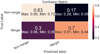 |
Fig. A.1. Total combined confusion matrix for the 10 runs of our Zoobot fine-tuning process. Each run fine-tuned a new model on a different set of training/validation data, and the confusion matrices are on 10 different sets of testing data. The stellar mass distributions for merger and non-merger galaxies used for fine-tuning Zoobot. The maximum and minimum values for each cell are also indicated. |
Appendix B: Predictions from simulation images
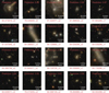 |
Fig. B.1. 20 randomly drawn examples of true positive classifications (merger probability > 0.5) from the 10 test sets, in descending order, with the probabilities indicated in the image, and the identification of the galaxy indicated below the image in the format [snapshot]-[ID]_[viewing angle]. The model seems to be able to identify various merger features, including close companions and merger remnants such as rings. |
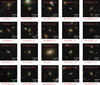 |
Fig. B.2. Same as Fig. B.1 but for true negatives. The model seems to be able to correctly identify some projections/overlaps as non-interacting. More importantly, a diverse appearance of non-mergers are correctly identified. |
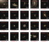 |
Fig. B.3. Same as Fig. B.1 but for false positives. Some close overlaps are incorrectly classified as a merging. Such galaxies, such as 84-432385_v2 with a merger probability of 0.90, would also likely be classified as mergers by human visual identification. |
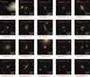 |
Fig. B.4. Same as Fig. B.1 but for false negatives. Many galaxies with lower probabilities, especially those in the bottom two rows are minor or mini mergers with the most recent/next merger close to the 0.5 Gyr threshold for merger selection. |
Appendix C: Predictions from observation images
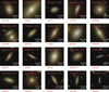 |
Fig. C.1. 20 randomly drawn examples of GAMA galaxies with a merger probability < 0.3, with merger probabilities in descending order. The merger probabilities are indicated in the image and the GAMA ID below the image. |
Appendix D: Fixed-mass environment trends
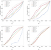 |
Fig. D.1. Cumulative distribution curves of merger probabilities of HSC galaxies cross-matched with GAMA (dotted lines) and SDSS (solid lines) predicted by our fine-tuned model, similar to Fig. 8, but separated into different mass bins. The KS test statistic between the most underdense and most overdense environments are also indicated for each subplot, with p-values available if > 0.05. Calculated for a 100 kpc radius aperture, in the following mass bins. 9 < log(M*) < 9.5 (upper left panel): KS test (SDSS) statistic: 0.432, KS test (GAMA) statistic: 0.263. 9.5 < log(M*) < 10 (upper right panel): KS test (SDSS) statistic: 0.601, KS test (GAMA) statistic: 0.378. 10 < log(M*) < 10.5 (lower left panel: KS test (SDSS) statistic: 0.757, KS test (GAMA) statistic: 0.053. 10.5 < log(M*) < 11 (lower right panel): KS test (SDSS) statistic: 0.064 p-value: 0.430, KS test (GAMA) statistic: 0.192. |
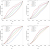 |
Fig. D.2. Same as Fig. D.1 but for a 500 kpc radius aperture. 9 < log(M*) < 9.5 (upper left panel): KS test (SDSS) statistic: 0.483, KS test (GAMA) statistic: 0.190. 9.5 < log(M*) < 10 (upper right panel): KS test (SDSS) statistic: 0.455, KS test (GAMA) statistic: 0.193. 10 < log(M*) < 10.5 (lower left panel): KS test (SDSS) statistic: 0.492, KS test (GAMA) statistic: 0.434, p-value: 0.503. 10.5 < log(M*) < 11 (lower right panel) KS test (SDSS) statistic: 0.233, KS test (GAMA) statistic: 0.159. |
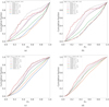 |
Fig. D.3. Same as Fig. D.1 but for a 1 Mpc radius aperture. 9 < log(M*) < 9.5 (upper left panel): KS test (SDSS) statistic: 0.436, KS test (GAMA) statistic: 0.211. 9.5 < log(M*) < 10 (upper right panel): KS test (SDSS) statistic: 0.473, KS test (GAMA) statistic: 0.156. 10 < log(M*) < 10.5 (lower left panel): KS test (SDSS) statistic: 0.352, KS test (GAMA) statistic: 0.113. 10.5 < log(M*) < 11 (lower right panel): KS test (SDSS) statistic: 0.241, KS test (GAMA) statistic: 0.137. |
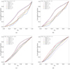 |
Fig. D.4. Same as Fig. D.1 but for a 8 Mpc radius aperture. 9 < log(M*) < 9.5 (upper left panel): KS test (SDSS) statistic: 0.193, p-value: 0.459, KS test (GAMA) statistic: 0.053, p-value: 0.767. 9.5 < log(M*) < 10 (upper right panel): KS test (SDSS) statistic: 0.170, p-value: 0.111, KS test (GAMA) statistic: 0.036, p-value: 0.822. 10 < log(M*) < 10.5 (lower left panel): KS test (SDSS) statistic: 0.107, p-value: 0.143, KS test (GAMA) statistic: 0.125, p-value: 7.059 × 10⁻⁷. 10.5 < log(M*) < 11 (lower right panel): KS test (SDSS) statistic: 0.200, KS test (GAMA) statistic: 0.255. |
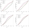 |
Fig. D.5. Same as Fig. D.1 but for an aperture of radius up to the fifth nearest neighbor. 9 < log(M*) < 9.5 (upper left panel): KS test (SDSS) statistic: 0.423, KS test (GAMA) statistic: 0.094. 9.5 < log(M*) < 10 (upper right panel): KS test (SDSS) statistic: 0.220, KS test (GAMA) statistic: 0.091. 10 < log(M*) < 10.5 (lower left panel): KS test (SDSS) statistic: 0.152, KS test (GAMA) statistic: 0.037, p-value: 0.045. 10.5 < log(M*) < 11 (lower right panel): KS test (SDSS) statistic: 0.190, KS test (GAMA) statistic: 0.075. |
All Tables
Means of metrics of ten individual Zoobot fine-tuning runs, assuming a complete binary class split (non-merger class (class 0): merger probability < 0.5, merger class (class 1): merger probability > 0.5).
All Figures
|
Fig. 1. Stellar mass distributions for the simulated TNG50 merger and non-merger galaxies used for fine-tuning Zoobot. There are 291 each of mergers and non-mergers, with 104 at z = 0.3. 111 at z = 0.2, and 76 at z = 0.1. Each merger galaxy used in the fine-tuning process has a corresponding non-merger galaxy at the same snapshot with a stellar mass within 0.1 dex. |
| In the text | |
|
Fig. 2. Merger probability distributions for TNG50 synthetic galaxy images predicted using our fine-tuned model. We used ten-fold cross-validation during training for ten independent testing samples to find probabilities for all galaxies, so that each galaxy was given one probability during the process. Each subfigure shows the merger probability distributions for different types of ground-truth mergers. (a) All galaxies, mergers, and non-mergers. (b) Non-mergers, pre-mergers (0.5 Gyr > time until merger > 0 Gyr), and post-mergers (0.5 Gyr > time since merger > 0 Gyr). (c) Non-mergers, major mergers (mass ratio > 1:4), minor mergers (1:4 > mass ratio > 1:10), mini mergers (1:10 > mass ratio > 1:20). |
| In the text | |
|
Fig. 3. Trained model’s ROC curve. The numbers overlayed on the curve indicate thresholds where the false positive and true positive rates along the curve are recorded. The dotted diagonal line is the performance of a completely random model that outputs a random probability for any image. An ROC curve is preferred to be above this dotted diagonal, and the curve generated from our model is above this line. We also find an AUC value of 0.84. |
| In the text | |
|
Fig. 4. Precision and completeness curves of the TNG images, with mean completeness and prevision as a function of merger probability. Left panel: curves assuming a complete binary split. The blue curve indicates completeness, and the orange curve indicates precision. Vertical error bars indicate the maximum and minimum values for the metric from the ten runs at each probability bin. Right panel: curves taking into consideration differing merger mass ratios (major, minor, mini). We find mini and minor mergers are predicted at an equivalent, if not greater precision compared to major mergers. We also find that the completeness at any fixed merger probability decreases with decreasing merger mass ratio. |
| In the text | |
|
Fig. 5. Merger probability distributions for HSC-SDSS (upper) and HSC-GAMA (lower) cross-matched galaxies predicted using our fine-tuned model. Note that in both cases, more galaxies lie in an unclear range (merger probability 0.2 − 0.5) for non-mergers than “confident” non-mergers (merger probability 0 − 0.1). However, we find that many of the mergers identified are confident (merger probability > 0.8). |
| In the text | |
|
Fig. 6. Merger probability distributions for galaxies with a spectroscopically identified pair within a 30 kpc radius aperture, binned by velocity difference of the pair. The vertical axis represents the fraction of galaxies in each merger probability bin belonging to each velocity difference bin. We find that the fraction of smaller velocity difference galaxy pairs increases monotonically with merger probability bin. |
| In the text | |
|
Fig. 7. Merger fraction as a function of merger probability for our two samples. The black vertical dotted line indicates the “confident” merger probability threshold of 0.8. We also plot the merger fractions found in Pearson et al. (2019b, red, green, and yellow lines), Nevin et al. (2023, brown lines), Kim et al. (2021, black lines), Lotz et al. (2011, light blue dotted line), and Cotini et al. (2013, purple line). We find that our merger fraction matches those of previous studies at increased merger probabilities. |
| In the text | |
|
Fig. 8. Cumulative distribution curves of merger probabilities of HSC galaxies cross-matched with GAMA (dotted lines) and SDSS (solid lines) predicted by our fine-tuned model, for environmental densities at differing apertures. log(1 + δ5) Each curve represents a different environmental density bin. The gradients of these curves show that in lower density environments, there are more higher merger probability galaxies, and in higher density environments, there are more galaxies with lower merger probabilities. This trend holds true for each parameter investigated. The trend also holds qualitatively between the SDSS and GAMA samples. The environmental parameters are as follows, and we also indicate the KS test statistic between the densest and least dense regions in each figure as reference. Upper left panel: 0.1 h−1 Mpc stellar mass overdensity log(1 + δ0.1 h−1 Mpc), KS test (SDSS) statistic: 0.394, KS test (GAMA) statistic: 0.238. Upper right panel: 0.5 h−1 Mpc stellar mass overdensity log(1 + δ0.5 h−1 Mpc), KS test (SDSS) statistic: 0.417, KS test (GAMA) statistic: 0.184. Middle left panel: 1 h−1 Mpc stellar mass overdensity log(1 + δ1 h−1 Mpc), KS test (SDSS) statistic: 0.341, KS test (GAMA) statistic: 0.143. Middle right panel: 8 h−1 Mpc stellar mass overdensity log(1 + δ8 h−1 Mpc), KS test (SDSS) statistic: 0.183, KS test (GAMA) statistic: 0.127. Bottom panel: fifth nearest neighbor mass overdensity, KS test (SDSS) statistic: 0.191, KS test (GAMA) statistic: 0.069. |
| In the text | |
|
Fig. 9. Environment distribution cumulative histograms of the environmental densities within a spherical volume including the fifth nearest neighbor to the target galaxy, for TNG50 and TNG100 mergers and non-mergers. From left to right: (a) environmental mass densities taking into account companions with mass ratio > 1:4 (major companions), and (b) environmental mass densities taking into account companions with mass ratio > 1:10 (major and minor companions). We also make the histograms for the observational data visible as reference where available, indicated by the dotted lines. KS test statistics between simulation mergers and non-mergers, as well as between confident mergers (merger probability > 0.8) and non-mergers (merger probability < 0.3) are indicated. Major companions (left panel): KS test (Simulation) statistic: 0.226, KS test (Observation) statistic: 0.131. Major and minor companions (right panel): KS test (Simulation) statistic: 0.194, KS test (Observation) statistic: 0.131. |
| In the text | |
|
Fig. 10. Same as Fig. 9, but for stellar mass overdensities within a 50 kpc radii spherical volume. Major companions (left panel): KS test (Simulation) statistic: 0.348. Major and minor companions (right panel): KS test (Simulation) statistic: 0.353. |
| In the text | |
|
Fig. 11. Same as Fig. 9, but for stellar mass overdensities within a 100 kpc radii spherical volume. Observational data are available for this parameter. Major companions (left panel): KS test (Simulation) statistic: 0.285, KS test (Observation) statistic: 0.231. Major and minor companions (right panel): KS test (Simulation) statistic: 0.260, KS test (Observation) statistic: 0.231. |
| In the text | |
|
Fig. 12. Same as Fig. 9, but for stellar mass overdensities within a 500 kpc radii spherical volume. Observational data are available for this parameter. Major companions (left panel): KS test (Simulation) statistic: 0.108, KS test (Observation) statistic: 0.171. Major and minor companions (right panel): KS test (Simulation) statistic: 0.100, KS test (Observation) statistic: 0.171. |
| In the text | |
|
Fig. 13. Same as Fig. 9, but for stellar mass overdensities within a 1 Mpc radii spherical volume. Observational data are available for this parameter. Major companions (left panel): KS test (Simulation) statistic: 0.140, KS test (Observation) statistic: 0.168. Major and minor companions (right panel): KS test (Simulation) statistic: 0.129, KS test (Observation) statistic: 0.168. |
| In the text | |
|
Fig. 14. Same as Fig. 9, but for stellar mass overdensities within a 2 Mpc radii spherical volume. Major companions (left panel): KS test (Simulation) statistic: 0.147. Major and minor companions (right panel): KS test (Simulation) statistic: 0.131. |
| In the text | |
|
Fig. 15. Same as Fig. 9, but for stellar mass overdensities within a 8 Mpc radii spherical volume. Observational data are available for this parameter. Major companions (left panel): KS test (Simulation) statistic: 0.153, KS test (Observation) statistic: 0.102. Major and minor companions (right panel): KS test (Simulation) statistic: 0.123, KS test (Observation) statistic: 0.102. |
| In the text | |
|
Fig. A.1. Total combined confusion matrix for the 10 runs of our Zoobot fine-tuning process. Each run fine-tuned a new model on a different set of training/validation data, and the confusion matrices are on 10 different sets of testing data. The stellar mass distributions for merger and non-merger galaxies used for fine-tuning Zoobot. The maximum and minimum values for each cell are also indicated. |
| In the text | |
|
Fig. B.1. 20 randomly drawn examples of true positive classifications (merger probability > 0.5) from the 10 test sets, in descending order, with the probabilities indicated in the image, and the identification of the galaxy indicated below the image in the format [snapshot]-[ID]_[viewing angle]. The model seems to be able to identify various merger features, including close companions and merger remnants such as rings. |
| In the text | |
|
Fig. B.2. Same as Fig. B.1 but for true negatives. The model seems to be able to correctly identify some projections/overlaps as non-interacting. More importantly, a diverse appearance of non-mergers are correctly identified. |
| In the text | |
|
Fig. B.3. Same as Fig. B.1 but for false positives. Some close overlaps are incorrectly classified as a merging. Such galaxies, such as 84-432385_v2 with a merger probability of 0.90, would also likely be classified as mergers by human visual identification. |
| In the text | |
|
Fig. B.4. Same as Fig. B.1 but for false negatives. Many galaxies with lower probabilities, especially those in the bottom two rows are minor or mini mergers with the most recent/next merger close to the 0.5 Gyr threshold for merger selection. |
| In the text | |
|
Fig. C.1. 20 randomly drawn examples of GAMA galaxies with a merger probability < 0.3, with merger probabilities in descending order. The merger probabilities are indicated in the image and the GAMA ID below the image. |
| In the text | |
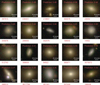 |
Fig. C.2. Same as Fig. C.1 but for merger probability > 0.3 and < 0.5. |
| In the text | |
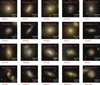 |
Fig. C.3. Same as Fig. C.1 but for merger probability > 0.5 and < 0.8. |
| In the text | |
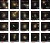 |
Fig. C.4. Same as Fig. C.1 but for merger probability > 0.8. |
| In the text | |
|
Fig. D.1. Cumulative distribution curves of merger probabilities of HSC galaxies cross-matched with GAMA (dotted lines) and SDSS (solid lines) predicted by our fine-tuned model, similar to Fig. 8, but separated into different mass bins. The KS test statistic between the most underdense and most overdense environments are also indicated for each subplot, with p-values available if > 0.05. Calculated for a 100 kpc radius aperture, in the following mass bins. 9 < log(M*) < 9.5 (upper left panel): KS test (SDSS) statistic: 0.432, KS test (GAMA) statistic: 0.263. 9.5 < log(M*) < 10 (upper right panel): KS test (SDSS) statistic: 0.601, KS test (GAMA) statistic: 0.378. 10 < log(M*) < 10.5 (lower left panel: KS test (SDSS) statistic: 0.757, KS test (GAMA) statistic: 0.053. 10.5 < log(M*) < 11 (lower right panel): KS test (SDSS) statistic: 0.064 p-value: 0.430, KS test (GAMA) statistic: 0.192. |
| In the text | |
|
Fig. D.2. Same as Fig. D.1 but for a 500 kpc radius aperture. 9 < log(M*) < 9.5 (upper left panel): KS test (SDSS) statistic: 0.483, KS test (GAMA) statistic: 0.190. 9.5 < log(M*) < 10 (upper right panel): KS test (SDSS) statistic: 0.455, KS test (GAMA) statistic: 0.193. 10 < log(M*) < 10.5 (lower left panel): KS test (SDSS) statistic: 0.492, KS test (GAMA) statistic: 0.434, p-value: 0.503. 10.5 < log(M*) < 11 (lower right panel) KS test (SDSS) statistic: 0.233, KS test (GAMA) statistic: 0.159. |
| In the text | |
|
Fig. D.3. Same as Fig. D.1 but for a 1 Mpc radius aperture. 9 < log(M*) < 9.5 (upper left panel): KS test (SDSS) statistic: 0.436, KS test (GAMA) statistic: 0.211. 9.5 < log(M*) < 10 (upper right panel): KS test (SDSS) statistic: 0.473, KS test (GAMA) statistic: 0.156. 10 < log(M*) < 10.5 (lower left panel): KS test (SDSS) statistic: 0.352, KS test (GAMA) statistic: 0.113. 10.5 < log(M*) < 11 (lower right panel): KS test (SDSS) statistic: 0.241, KS test (GAMA) statistic: 0.137. |
| In the text | |
|
Fig. D.4. Same as Fig. D.1 but for a 8 Mpc radius aperture. 9 < log(M*) < 9.5 (upper left panel): KS test (SDSS) statistic: 0.193, p-value: 0.459, KS test (GAMA) statistic: 0.053, p-value: 0.767. 9.5 < log(M*) < 10 (upper right panel): KS test (SDSS) statistic: 0.170, p-value: 0.111, KS test (GAMA) statistic: 0.036, p-value: 0.822. 10 < log(M*) < 10.5 (lower left panel): KS test (SDSS) statistic: 0.107, p-value: 0.143, KS test (GAMA) statistic: 0.125, p-value: 7.059 × 10⁻⁷. 10.5 < log(M*) < 11 (lower right panel): KS test (SDSS) statistic: 0.200, KS test (GAMA) statistic: 0.255. |
| In the text | |
|
Fig. D.5. Same as Fig. D.1 but for an aperture of radius up to the fifth nearest neighbor. 9 < log(M*) < 9.5 (upper left panel): KS test (SDSS) statistic: 0.423, KS test (GAMA) statistic: 0.094. 9.5 < log(M*) < 10 (upper right panel): KS test (SDSS) statistic: 0.220, KS test (GAMA) statistic: 0.091. 10 < log(M*) < 10.5 (lower left panel): KS test (SDSS) statistic: 0.152, KS test (GAMA) statistic: 0.037, p-value: 0.045. 10.5 < log(M*) < 11 (lower right panel): KS test (SDSS) statistic: 0.190, KS test (GAMA) statistic: 0.075. |
| In the text | |
Current usage metrics show cumulative count of Article Views (full-text article views including HTML views, PDF and ePub downloads, according to the available data) and Abstracts Views on Vision4Press platform.
Data correspond to usage on the plateform after 2015. The current usage metrics is available 48-96 hours after online publication and is updated daily on week days.
Initial download of the metrics may take a while.