| Issue |
A&A
Volume 697, May 2025
|
|
|---|---|---|
| Article Number | A145 | |
| Number of page(s) | 13 | |
| Section | Extragalactic astronomy | |
| DOI | https://doi.org/10.1051/0004-6361/202452454 | |
| Published online | 14 May 2025 | |
Revisiting the globular clusters of NGC 1052-DF2⋆
1
Department of Astrophysics, University of Vienna, Türkenschanzstraße 17, 1180 Wien, Austria
2
European Space Agency, European Space Research and Technology Centre, Keplerlaan 1, 2201 AZ Noordwijk, The Netherlands
3
Instituto de Astrofísica de Canarias, Calle Vía Láctea, E-38206 La Laguna, Spain
4
Departamento de Astrofísica, Universidad de La Laguna, E-38206 La Laguna, Spain
5
Centre for Astrophysics and Supercomputing, Swinburne University, John Street, Hawthorn, VIC 3122, Australia
6
Department of Physics, Centre for Extragalactic Astronomy, Durham University, South Road, Durham DH1 3LE, UK
7
European Southern Observatory, Karl-Schwarzschild-Strasse 2, 85748 Garching bei München, Germany
8
Department of Theoretical Physics and Astrophysics, Faculty of Science, Masaryk University, Kotlářská 2, Brno 611 37, Czech Republic
9
Univ. Lyon, ENS de Lyon, Univ. Lyon1, CNRS, Centre de Recherche Astrophysique de Lyon, UMR5574, 69007 Lyon, France
⋆⋆ Corresponding author: This email address is being protected from spambots. You need JavaScript enabled to view it.
Received:
1
October
2024
Accepted:
14
March
2025
Abstract
The ultra-diffuse galaxy (UDG) NGC 1052-DF2 has captured the interest of astronomers ever since the low velocity dispersion measured from ten globular clusters (GCs) suggested a low dark matter fraction. Also, its GC system was found to be unusually bright, with a GC luminosity function peak at least one magnitude brighter than expected for a galaxy at a distance of 20 Mpc. In this work we present an updated view of the GC system of NGC 1052-DF2. We analysed archival MUSE data of NGC 1052-DF2 to confirm the membership of four additional GCs based on their radial velocities, thereby raising the number of spectroscopically confirmed GCs to 16. We measured the ages and metallicities of 11 individual GCs, finding them to be old (> 9 Gyr) and with a range of metallicities from [M/H] = −0.7 to −1.8 dex. The majority of GCs are found to be more metal-poor than the host galaxy, with some metal-rich GCs sharing the metallicity of the host ([M/H] = −1.09−0.07+0.09 dex). The host galaxy shows a flat age and metallicity gradient out to 1 Re. Using a distance measurement based on the internal GC velocity dispersions (D = 16.2 Mpc), we derived photometric GC masses and find that the peak of the GC mass function compares well with that of the Milky Way. From updated GC velocities, we estimated the GC system velocity dispersion of NGC 1052-DF2 with a simple kinematic model and find σGCS = 14.86−2.83+3.89 km s−1. However, this value is reduced to σGCS = 8.63−2.14+2.88 km s−1 when the GC that has the highest relative velocity based on a low S/N spectrum is considered an interloper. We discuss the possible origin of NGC 1502-DF2, taking the lower distance, spread in GC metallicities, flat stellar population profiles, and dynamical mass estimate into consideration.
Key words: galaxies: individual: NGC 1052-DF2 / galaxies: star clusters: general
Based on observations made with ESO Telescopes at the La Silla Paranal Observatory under programmes ID 2101.B-5008(A) and 110.23P4.001.
© The Authors 2025
 Open Access article, published by EDP Sciences, under the terms of the Creative Commons Attribution License (https://creativecommons.org/licenses/by/4.0), which permits unrestricted use, distribution, and reproduction in any medium, provided the original work is properly cited.
This article is published in open access under the Subscribe to Open model. This email address is being protected from spambots. You need JavaScript enabled to view it. to support open access publication.
1. Introduction
Ultra-diffuse galaxies (UDGs) are a subclass of low-surface-brightness (LSB) galaxies characterised by their low luminosities and surface brightness (μg > 24 mag arcsec−2) and large effective radii (Re > 1.5 kpc; van Dokkum et al. 2015). While the first examples of such galaxies were found in the 1980s (e.g. Sandage & Binggeli 1984; Impey et al. 1988; Dalcanton et al. 1997; Impey & Bothun 1997; Conselice et al. 2003), UDGs have received a lot of attention in the last decade thanks to ever more sensitive telescopes and deep photometric surveys (e.g. Janssens et al. 2017; Prole et al. 2019; Zaritsky et al. 2019; Iodice et al. 2020; Zaritsky et al. 2023; Janssens et al. 2024). Consequently, thousands of UDGs are now known, although the sample with available spectroscopy is notably smaller (but see for example Ferré-Mateu et al. 2023; Iodice et al. 2023; Gannon et al. 2024; Ferré-Mateu et al. 2025).
One UDG in particular has sparked a lot of interest from the research community: NGC 1052-DF2 (also catalogued as KKSG04, PGC3097693, and [KKS2000]04; Karachentsev et al. 2000). Using Keck Low Resolution Imaging Spectrometer (LRIS) and DEep Imaging Multi-Object Spectrograph (DEIMOS) spectra of ten luminous globular clusters (GCs), van Dokkum et al. (2018a,b) found a surprisingly small velocity dispersion, < 10 km s−1, suggesting a very low or even negligible fraction of dark matter (DM) contributing to the total mass of this galaxy.
At the same time, Hubble Space Telescope (HST) photometry showed that NGC 1052-DF2 has an extremely luminous GC system (GCS) with a GC luminosity function (GCLF) turnover magnitude at least one magnitude brighter than expected if the galaxy is placed at ∼20 Mpc, the distance of the NGC 1052 group (van Dokkum et al. 2018c). To reconcile both the lack of DM and the luminous GCS, Trujillo et al. (2019) proposed that a distance of about 13 Mpc. At this distance, NGC 1052-DF2 would be a more ordinary LSB galaxy. This lower distance was disputed with newer and deeper HST data by Shen et al. (2021a), who measured a distance of D = 22.1 ± 1.2 Mpc based on the tip of the red giant branch (TRGB; see also van Dokkum et al. 2018d). In Shen et al. (2023), this distance was revised to D = 21.7 Mpc to account for an incorrect alignment of the HST data. Using the same deep data, Shen et al. (2021b) show that this larger distance places the peak of the GCLF about 1.5 magnitudes brighter than the universal value of MV = −7.5 mag. To add to these puzzling results, van Dokkum et al. (2022a) find that the spectroscopically confirmed GCs all have very similar V − I colours. They suggest that this is in line with a proposed formation scenario for NGC 1052-DF2 and the UDG NGC 1502-DF4, in which both galaxies formed after the collision of gas-rich progenitor galaxies (van Dokkum et al. 2022b; Tang et al. 2025). Using a theoretical model, Trujillo-Gomez et al. (2021) also propose that the luminous GCS could have formed at very high gas densities, possibly in a major merger.
Beyond the original spectroscopic sample of ten GCs, Trujillo et al. (2019) present additional GC candidates, one of which was later confirmed as a GC by Emsellem et al. (2019). These authors used deep integral field spectroscopy (IFS) with the Multi Unit Spectroscopic Explorer (MUSE; Bacon et al. 2010) to analyse the stellar body of NGC 1052-DF2 and its GCS, confirming the low GCS velocity dispersion and finding a low velocity dispersion of the stars as well as indications of low-level stellar rotation. This small velocity dispersion of the stellar body was also found with Keck Cosmic Web Imager (KCWI) IFS by Danieli et al. (2019), who did not detect rotation in their smaller field of view.
Fensch et al. (2019) present an analysis of the stellar population properties of the host galaxy and the GCS based on the MUSE data. From an integrated spectrum of the stellar component and a stacked spectrum of the GCs within the MUSE field of view, they find old ages (∼9 Gyr). The stars appear to be more metal-rich ([M/H] = −1.07 ± 0.12 dex) than the GCs ([M/H] = −1.63 ± 0.09 dex). Similar values were found using slit spectroscopy by Ruiz-Lara et al. (2019). From stacked Keck LRIS spectra, van Dokkum et al. (2018c) also find an old age (> 9 Gyr) for the GCs but a higher average metallicity ([Fe/H] = −1.35 ± 0.12 dex).
We re-analysed the MUSE data to confirm four additional GC candidates and to determine the ages and metallicities of individual GCs rather than stacked spectra. Complementary, an accompanying paper (Beasley et al. 2025, hereafter Paper I) presents the analysis of high-resolution FLAMES spectra. From measurements of the intrinsic GC velocity dispersion, Paper I presents an independent measurement of the distance to NGC 1052-DF2 using the GC velocity dispersion distance method (Beasley et al. 2024), finding 16.2 ± 1.3 (stat.) ± 1.1 (sys.) Mpc. This method employs the relation between GC absolute magnitude and internal velocity dispersion to determine the distance. As described in Beasley et al. (2024), the relation was calibrated using GCs of the Milky Way and M 31 and was successfully applied to Centaurus A and Local Group dwarfs using literature data. In Paper I this method was applied to NGC 1502-DF2, a much more distant galaxy. The found distance is at odds with the TRGB measurement, and as discussed in Paper I no definitive reason for this discrepancy is found. Paper I employs the metallicity measurements presented here and notes that intrinsic properties of the GCs (e.g. their mass-to-light ratios as derived from the MUSE spectra) agree with those of Milky Way GCs. A vastly different initial mass function might influence the results but only in combination with younger cluster ages, which are are disfavoured by the stellar population results presented here. Nonetheless, other as yet undiscovered systematic effects might influence this distance measurement. For consistency with Paper I, we assume a distance of 16.2 Mpc in the following but also discuss any distance-dependent results using the TRGB distance of 21.7 Mpc. Combining the FLAMES results with the analysis of the MUSE data described here, we present an updated view of NGC 1052-DF2 and its GCS.
2. Data
We used the fully reduced MUSE data as provided by Emsellem et al. (2019). The data consist of seven observing blocks amounting to 5.1 h exposure time on target (programme 2101.B-5008(A)). The data were reduced following standard recipes including bias, flat fielding, wavelength calibration, and line spread function corrections using the dedicated python package PYMUSEPIPE1. Sky lines were removed using dedicated sky observations and residual sky lines were further cleaned by using the Zurich Atmosphere Purge (ZAP) code (Soto et al. 2016). Emsellem et al. (2019) provide different versions of the reduced data using different sky subtraction parameters. In this work, we used the linearly sampled, sky-subtracted version that was constructed using a 50 pixel continuum window in ZAP.
The data cube covers a ∼1′× 1′ field of view, sampled at 0.2″ pix−1 and with a point spread function (PSF) full width at half maximum (FWHM) of ∼0.8″. Along the wavelength direction, the cube covers the optical wavelength range from ∼4700 to 9300 Å with a sampling of 1.25 Å per pixel. As described in Emsellem et al. (2019), the line spread function varies from FWHM ∼2.9 Å at 5000 Å to ∼2.5 Å at 9000 Å but is well described by the UDF10 profile of Guérou et al. (2017), but not exactly the same as discussed in the appendix of Emsellem et al. (2019). Figure 1 shows a false-colour red-green-blue (RGB) image obtained from the MUSE data using MPDAF (Bacon et al. 2016) to obtain synthetic images in V, R, and I. The GCs analysed in this work are marked and labelled.
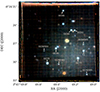 |
Fig. 1. RGB image of NGC 1052-DF2 created from the MUSE data. GCs analysed in this work are marked and labelled. Red: V, green: R, blue: I. See also Fensch et al. (2019). |
As detailed in Paper I, several GCs of NGC 1052-DF2 were observed with the FLAMES spectrograph. The spectra were taken with the H875.7 (HR21) grating that covers the Calcium triplet region (8500–9000 Å) and have a spectral resolution of 0.53 Å as measured from sky lines. Paper I focused on deriving the GC velocity dispersion from the five brightest GCs, while we present the radial velocities of the full sample in this work. For details on the data reduction and analysis of the FLAMES spectra, we refer to Paper I.
3. Spectroscopic analysis
In the following, we describe our analysis of the analysis of the MUSE data. Firstly, we detail the extraction of GC spectra from the data and then describe the full spectrum fitting methods used to extract GC properties.
3.1. Extracting GC spectra from MUSE
To identify GCs in the data, we first constructed a white light image from the MUSE cube by integrating along the spectral axis. Using the DAOSTARFINDER routine implemented in PHOTUTILS (Bradley et al. 2023), we then detected all point sources 2σ above the background flux level as determined in a corner of the image. By cross-referencing those sources with previously confirmed GCs (van Dokkum et al. 2018c; Emsellem et al. 2019; Ruiz-Lara et al. 2019), we obtained the pixel centroids of GC73, GC77, GC85, GC92, GC93, GC98, and GCNEW3 (T3 in Emsellem et al. 2019), as well as the GC candidates GCNEW2, GCNEW4, GCNEW5, and GCNEW6 (Trujillo et al. 2019). Additionally, we added the coordinates of other bright point sources to check for yet undetected GCs.
To extract the spectra from MUSE, we used a similar method as in Fahrion et al. (2020a) and Fahrion et al. (2022). To boost the signal from the GCs, we first obtained a model with MPDAF of the wavelength-dependent PSF using a bright foreground star (the source originally named GCNEW7 in Trujillo et al. 2019). We used this PSF cube as weighting for each wavelength slice. This approach leads to a slightly improved signal-to-noise ratio (S/N) compared to using a single two-dimensional Gaussian. The improvement is between 5 and 10%. We also extracted a spectrum of the underlying galaxy in an annulus around each GC. After testing, we chose to not subtract this background spectrum from the GC spectra as the contrast between GCs and galaxy is large and subtraction would therefore only introduce noise. Nonetheless, the derived properties remain even when subtracting the background spectrum, but with larger uncertainties. Except for the faint source GCNEW6 (S/N ∼ 5), the resulting spectra have signal-to-noise values between 10 and 50 per pixel. As shown in the appendix of Fahrion et al. (2019), such a S/N is sufficient to measure stellar population properties in addition to the line-of-sight velocities. For this reason, we chose to derive ages and metallicities of individual GCs rather than using a stacked spectrum as done by Fensch et al. (2019) and van Dokkum et al. (2018c).
Spectroscopically confirmed GCs.
3.2. Full spectrum fitting with PPXF
We used the Penalized PiXel-Fitting (PPXF) method (Cappellari & Emsellem 2004; Cappellari 2017, 2023) to fit the MUSE spectra. Using a penalised pixel fitting approach, PPXF fits a spectrum by finding the best-fitting linear combination of user-supplied models. PPXF allows the parameters of the line-of-sight velocity distribution to be measured, such as radial velocity and velocity dispersion. Additionally, PPXF returns the weights of the models used in the best fit and so the best-fitting age and metallicity can be reconstructed.
To fit the MUSE spectra, we used the EMILES single stellar population (SSP)2 models (Vazdekis et al. 2010, 2016) that are based on the MILES stellar spectra. The models are similar to those used by Emsellem et al. (2019) and Fensch et al. (2019); however, we used the models based on the BaSTI isochrones (Pietrinferni et al. 2004, 2006) with a double power-law initial mass function with high-mass slope of 1.30 (Vazdekis et al. 1996), rather than the Padova isochrones. The models cover ages from 30 Myr to 14 Gyr and total metallicities between [M/H] = −2.27 dex and +0.40 dex.
During the fit, we used a two step approach: First, we fitted for the line-of-sight velocities using additive polynomials of degree 12. In the second step, the velocity is kept fixed and no additive polynomials are used. Instead, multiplicative polynomials of degree 8 are used to minimise template mismatch. From the returned weights, we inferred age and metallicity of the best-fitting spectrum. In the fit, sky residual lines are masked and a broad wavelength range from 4750 to 8750 Å was used. Figure 2 shows the blue part of the MUSE spectra and the PPXF fits.
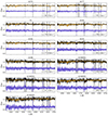 |
Fig. 2. Full spectrum fitting of the GCs. Each panel shows the GC spectrum in black and the pPXF fit in orange. The respective residuals are shown in purple, shifted for visualisation. Grey shaded areas are regions masked from the fit due to sky residual or telluric lines. In the lower right corner, the best-fitting velocity is shown. The panels only show the blue part of the spectrum. |
To derive statistical uncertainties, we used a Monte Carlo (MC) approach. Here, we perturbed the best-fitting spectrum with randomly drawn noise from the residual (best fit subtracted from original spectrum) to create 100 representations of the spectrum. Those are fitted to obtain histograms of velocity, age, and metallicity. The reported values in Tables 1 and 2 refer to the 16th, 50th, and 84th percentiles of these distributions.
Globular clusters in the MUSE field of view.
As described in Paper I, we also fitted the FLAMES spectra with PPXF. To get reliable velocity dispersion measurements, we used empirical stellar spectra that have to be brought to an arbitrary common velocity to be used as models. Here, however, we focus solely on the radial velocities and therefore used the high-resolution models from Coelho (2014) with metallicities [Fe/H] ≤ −1.0 dex. The line-of-sight velocities are reported in Table 1. Figure 1 in Paper I shows two examples of the spectra.
3.3. Confirming additional GC candidates
Beyond the already confirmed GCs, we found four additional sources in the MUSE data that have velocities in agreement with the systemic velocity of NGC 1052-DF2 (vsys = 1792.9 km s−1, Emsellem et al. 2019). Those are GCNEW2, GCNEW4, and GCNEW5 from the candidates of Trujillo et al. (2019) as well as one source that has not been listed yet. We name this source GCNEW9, following the naming scheme in Trujillo et al. (2019). The spectrum of GCNEW6 is rather noisy and while we find a velocity of v = 1856 km s−1, the uncertainty is above 50 km s−1. For this reason, we cannot confirm the nature of this source and do not include it in the following analysis.
From the FLAMES spectra, we could measure velocities of ten GCs, all previously confirmed as GCs. Unfortunately, the spectra of the GC candidates GCNEW1 and GCNEW8 are too noisy to obtain a velocity estimate as the uncertainties are above 20 km s−1. In our sample, we also include GC101. For this GC, we found a velocity of 1836.0 km s−1, which is the highest relative velocity of all GCs in the sample. As discussed below and in Paper I, this elevated velocity was found consistently when testing different fitting approaches, but due to the rather low S/N of 3, we cannot exclude that this velocity is affected by systematics or that at least the uncertainties are underestimated.
4. Results
With the four newly confirmed GCs, the sample of spectroscopically confirmed GCs of NGC 1052-DF2 is now 16. We list their coordinates, velocities, and apparent magnitudes in Table 1. In addition, Table 2 reports the stellar population results of the GCs within the MUSE data.
4.1. Comparison of radial velocities
We show a comparison of different GC velocity measurements in Fig. 3. In this figure, we compare our measurements from the MUSE spectra to the velocities obtained from the FLAMES spectra, as well as to the measurements from Emsellem et al. (2019) using the same MUSE data, and to the velocities from Keck DEIMOS and LRIS spectra (van Dokkum et al. 2018d,b). We find a good agreement between the velocities from MUSE and FLAMES; however, the measurements from FLAMES spectra have notably lower uncertainties. In addition, our measurements agree with those from Emsellem et al. (2019), with a larger scatter for the lower S/N clusters, possibly due to a slightly different spectrum extraction method. As also noted in Emsellem et al. (2019), there seems to be a consistent offset between the MUSE velocities and those from Keck DEIMOS and LRIS spectra of ∼12 km s−1. Emsellem et al. (2019) found an offset of 12.5 km s−1 and suggested that part of it is caused by the transformation between redshift and wavelengths. Apart from this offset, the GC velocities between MUSE and DEIMOS/LRIS spectra agree very well.
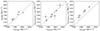 |
Fig. 3. Comparison of velocity measurements. Left: Comparison of GC velocities from this work based on the MUSE data and from the FLAMES spectra presented in Paper I. Middle: Comparison between this work and GC velocities from the same data as presented in Emsellem et al. (2019). Right: Comparison to GC velocities reported in van Dokkum et al. (2018a,b) from Keck DEIMOS and LRIS spectra. The dashed line shows the one-to-one relation, while the dotted line in the rightmost panel refers to a velocity offset of 12 km s−1 (see also Emsellem et al. 2019). |
4.2. Age metallicity distribution
Figure 4 shows the best-fitting ages and total metallicities of the analysed GCs, compared to results from van Dokkum et al. (2018c), Fensch et al. (2019), and Ruiz-Lara et al. (2019) based on stacked spectra. Using slit spectroscopy, Ruiz-Lara et al. (2019) found an average age of 8.7 ± 0.7 Gyr and a metallicity of [M/H] = −1.18 ± 0.05 dex, similar to the results from an aperture spectrum extracted from the MUSE data by Fensch et al. (2019). Additionally, Fensch et al. (2019) used the MUSE spectra of the six GCs presented in Emsellem et al. (2019) to create a stacked spectrum, weighted by S/N, and fitted with pPXF and the EMILES models. van Dokkum et al. (2018c) stacked LRIS-blue spectra of 11 GCs and fitted the spectrum with ALF (Conroy & van Dokkum 2012; Conroy et al. 2018) to obtain a best-fitting iron metallicity of [Fe/H] = −1.35 ± 0.12 dex, magnesium abundance of [Mg/Fe] = +0.16 ± 0.17 dex, and age = 9.3 Gyr. To compare these iron metallicities with the total metallicities used in EMILES, we used the relation [Fe/H]=[M/H]−0.75 × [Mg/Fe] as given on the MILES web page. As already noted by Fensch et al. (2019), their GC metallicity is lower than what was found by van Dokkum et al. (2018c) and they discussed multiple reasons for the difference in measured GC metallicity, including the different modelling approaches, different SSP models, and wavelength ranges.
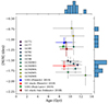 |
Fig. 4. Age versus metallicity of the GCs. Coloured dots refer to the MUSE GCs analysed here. The red cross shows the result from the stacked GC spectrum of Fensch et al. (2019), and the blue cross refers to the UDG itself as determined from an aperture spectrum. The dark red point shows the result from the stacked Keck spectra from van Dokkum et al. (2018c), and the green triangle shows the UDG metallicity from slit spectroscopy presented by Ruiz-Lara et al. (2019). |
With our individual measurements and improved GC number, we can now investigate the age-metallicity plane in greater detail. Overall, the GCs appear to be old with ages > 9 Gyr, similar to what was found from the stacked spectra. However, we observe a broad range of GC metallicities, ranging from [M/H] = −0.73 dex to −1.86 dex. Out of the eleven GCs in the MUSE field of view, seven have metallicities < − 1.50 dex, while the remaining four have higher metallicities. Interestingly, the metal-poor GCs appear to scatter around the average value found by Fensch et al. (2019), while the more metal-rich ones have similar metallicities as the UDG itself. Out of the GCs presented here, Fensch et al. (2019) included six metal-poor GCs (GC73, GC77, GC92, GC93, GC98, and T3) in their stack as well as the metal-rich GC85, which explains the low average metallicity. Nonetheless, due to the higher uncertainties of the individual GC metallicities, even the metal-rich ones agree with the stacked value within 3σ, with the exception of GCNEW5. van Dokkum et al. (2018c) included also GCs outside the MUSE field of view for which no individual metallicities are available. However, the higher average metallicity could be an indication that their stacked spectrum has also included a higher number of metal-rich GCs.
4.3. Colour–metallicity relation
We investigated the relationship between photometric colours and spectroscopic metallicities in Fig. 5. The slope of this so-called colour–metallicity relation (CZR) is important when photometric measurements are used as this relation allows one to translate from colours to the more fundamental property of metallicity (e.g. Usher et al. 2015; Fahrion et al. 2020b; Hartman et al. 2023).
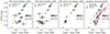 |
Fig. 5. CZR of the GCs. Each panel shows the spectroscopic metallicities versus HST F606W − F814W colour and predictions from the EMILES models colour-coded by age. From left to right: Colours from Paper I, Trujillo et al. (2019), van Dokkum et al. (2022a), and synthetic colours derived from the MUSE spectra directly. In the right panel, we also include the Fornax3D GC sample from Fahrion et al. (2020a). |
In Fig. 5 we show the GC metallicities versus VF606W − IF814W colours in the left panel. The photometric measurements stem from a new analysis of the deeper HST data (combining data from 2017 and 2020), as described in more detail in Paper I. Additionally, we compare those colours to the HST measurements using the original HST data from Trujillo et al. (2019) as well as the colours from van Dokkum et al. (2022a). The latter are also based on the deeper HST data, but the colours from van Dokkum et al. (2022a) are significantly bluer and span only a very narrow colour range. As also discussed in Paper I, we found F606W magnitudes that are ∼0.1 mag fainter than the ones reported in van Dokkum et al. (2022a), while the F814W magnitudes agree within our larger uncertainties. As a consequence, we found a larger spread in colours. The reason for this discrepancy is unknown, but might be related to a different approach to modelling the photometric data. Unfortunately, the photometric measurements of van Dokkum et al. (2022a) do not include the newly confirmed GCs that are more metal-rich, so the comparison to metallicities is restricted to only five GCs, four of which are metal-poor.
Additionally, we derived synthetic colours in the HST Advanced Camera for Surveys (ACS) F606W and F814W bands using SYNPHOT (STScI Development Team 2018) to convolve the MUSE spectra with the HST transmission curves. The same approach was taken to obtain colour predictions from the EMILES SSP models. As a comparison sample, we also obtained colours in the same bands from the spectra of the Fornax3D GC sample (Fahrion et al. 2020a), which provides a MUSE-based spectroscopic sample of 230 GCs with S/N > 8 around mainly massive early-type galaxies in the Fornax galaxy cluster. We note that the synthetic MUSE colours agree with the HST colours and compare well to the Fornax3D GC sample.
Irrespective of the differences in colours derived with different approaches, Fig. 5 clearly shows that a narrow range of colours does not necessarily imply a narrow range of metallicities. The reason for this is that at the blue colours of the NGC 1052-DF2 GCs, the CZR has a steep slope, as for example the large Fornax3D sample illustrates. The same is seen for the EMILES SSP predictions that can give an indication for the slope of the CZR, even though the SSPs do not cover all the aspects of true GCs3.
4.4. GC mass-to-light ratios and masses from stellar populations
Fitting the GC spectra for their ages and metallicities allows us to determine their mass-to-light ratios (M/L) as predicted from the EMILES SSP models. For this, we used the photometric predictions in the
HST ACS filter F606W that provide the mass-to-light ratio for every age and metallicity in the model grid. We used a two-dimensional interpolation to obtain the M/L for any given age and metallicity and used this to translate the MC distributions of age and metallicity to a M/L value for every MC fit. From this, we determined the M/L and its uncertainty. The results are reported in Table 1. The M/L values range from 1.25 to 2.04, similar to typical M/L values of GCs in the MW (Baumgardt & Hilker 2018) and also comparable to the dynamical M/L values derived from the FLAMES spectra, which have a mean V-band M/L = 1.61 ± 0.44 (Paper I).
To then estimate the stellar masses of the GCs, we used the GC apparent magnitudes from Paper I and assumed a distance of 16.2 Mpc (Paper I). For GCs outside the MUSE field of view without metallicities, we used the M/LF606W = 1.45, which corresponds to the median value. The resulting histogram of masses is shown in Fig. 6. We compare this histogram to Milky Way GCs from Baumgardt & Hilker (2018) (black curve), showing that the peak that the mass distribution of the NGC 1052-DF2 GCs analysed here is located at ∼105.4 M⊙ = 2.5 × 10⁵ M⊙, very close to the canonical peak of the GC mass function at MGC ∼ 2 × 10⁵ M⊙ (Harris 2010; Brodie & Strader 2006; Jordán et al. 2007). At a distance of 21.7 Mpc, the peak would be at higher masses of ∼4 × 10⁵ M⊙, as also noted by Shen et al. (2021b). We note that using the brighter F606W magnitudes presented in van Dokkum et al. (2022a) also changes the mass distribution. For example, using their magnitudes and a distance of 16.2 Mpc, the peak of the distribution is then placed at 2.9 × 10⁵ M⊙.
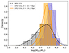 |
Fig. 6. Distribution of derived masses based on stellar population properties. The orange histogram shows the NGC 1052-DF2 GCs assuming a distance of 16.2 Mpc, and the orange line shows a kernel density estimation line to visualise the distribution. We note that the histogram only shows the spectroscopically confirmed GCs and that no completeness correction was applied. The purple histogram and corresponding dotted purple line shows the mass distribution assuming a larger distance of 21.7 Mpc. The grey histogram and the black line show the distribution of 112 GCs from the Milky Way from Baumgardt & Hilker (2018). |
4.5. Comparison to the stellar light
In their analysis of the MUSE data, Fensch et al. (2019) reported an average metallicity and age of the stellar light obtained from fitting an aperture spectrum within 1 Re (22″). Here, we provide more detail by extracting the galaxy spectrum in different annuli out to the effective radius. For this, we first masked GCs and other compact sources from the data cube (similar to Emsellem et al. 2019). Then, we extracted the galaxy spectrum in elliptical annuli with position angle = −48° and ellipticity ϵ = 0.15 (van Dokkum et al. 2018d; Emsellem et al. 2019). As annuli widths we chose 10 pix ( = 2″) out to 70 pix and then chose 20 pix for the two outermost bins due to the decreasing surface brightness. We then fitted the spectra with pPXF.
Figure 7 shows the radial profiles of metallicities and ages of the stellar light in comparison to the GCs. Within the uncertainties, both age and metallicity profiles appear to be flat, but there seems to be a mild trend of older ages at larger radii. While many low group dwarf galaxies are found to have negative metallicity gradients (e.g. Taibi et al. 2022), the UDG DF44 is also known to have a flat metallicity profile (Villaume et al. 2022). However, the sample of UDGs with spectroscopically measured stellar population gradients is very limited (see e.g. Gannon et al. 2024; Ferré-Mateu et al. 2025).
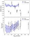 |
Fig. 7. Radial metallicity and age profiles. Top: Metallicity profile of the stellar light obtained from elliptical annuli spectra in blue and GC metallicities in black. Bottom: Age profile for the stars and the GCs. |
As noted before, the GCs are overall old, but scatter in metallicity over a wide range, with most being more metal-poor than the stars. In a galaxy with an extended star formation history, such a spread is expected. The more metal-rich GCs scatter around the metallicity of the host galaxy, as also often observed for more massive galaxies (e.g. Fahrion et al. 2020a). In addition to the annuli spectra, we also obtained integrated spectra within the effective radius. From this, we found [M/H] =  dex and Age =
  Gyr, in agreement with the findings from Fensch et al. (2019). For these values, the EMILES models predict a M/LF606W of 1.67 ±0.17 in the HST F606W filter. With an apparent magnitude of V = 16.1 mag (van Dokkum et al. 2018a), this mass-to-light ratio translates to a stellar mass of M* ∼ 1.1 × 10⁸ M⊙ at 16.2 Mpc, or M* ∼ 2 × 10⁸ M⊙ at 21.7 Mpc.
4.6. Simple kinematic model of the GC system
Combing the samples from MUSE and FLAMES, we now have a sample of 16 GCs in NGC 1052-DF that have precise velocity measurements available. For this reason, we model the kinematics of the GCS in a similar way as described in Martin et al. (2018), Laporte et al. (2019), Lewis et al. (2020), or Emsellem et al. (2019), but with an updated number of GCs. For our model, we used the same model as in Fahrion et al. (2020a), which follows the description in Veljanoski & Helmi (2016) and is comparable to the rotation model by Lewis et al. (2020). In the model, the global rotation of the GCS is described as (Côté et al. 2001)
 (1)
(1)
where vGC,i is the velocity of the ith GC at a position angle of θi, vsys the systemic velocity of the galaxy and VGCS the rotation amplitude. θ0 describes the angle of the rotation axis, where the rotation is maximum at θ0 + 90°. In this model, only the global rotation and dispersion is described and it assumes that those do not vary with radius.
Assuming that the intrinsic velocity dispersion σGCS is well represented by a Gaussian, it can be described as
 (2)
(2)
where δvGC,i is the velocity uncertainty of the ith GC. We then write the likelihood function as
 (3)
(3)
As input to this model, we derived the position angles θi of the GCs from the north going counter-clockwise and assuming a galaxy centre at RA = 02:41:46.80, Dec = −08:24:09.3. For the velocities, we used the FLAMES velocities where available and the MUSE velocities for the rest. The uncertainties were converted to symmetric values by taking the mean between lower and upper uncertainty.
We implemented the model in EMCEE (Foreman-Mackey et al. 2013), a python module that implements a Markov chain Monte Carlo sampler. We used flat priors for all free parameters (vSYS, VGCS, σ, θ0). We restricted the position angle to be between 0 and 180°, but allowed the rotation amplitude to also take negative values to describe counter-rotation.
Figure 8 shows the posterior distributions of the fit. The parameters are well constrained, except for the position angle due to the low amplitude of rotation. We find a systemic velocity of  km s−1, a rotation amplitude in agreement with zero, and a GCS velocity dispersion of
  km s−1. Testing a model without rotation as described, for example in Emsellem et al. (2019), we find similar values for the velocity dispersion. This value is higher than what was reported originally by van Dokkum et al. (2018a), who found an intrinsic velocity dispersion of
  km s−1 that was later revised to
  km s−1 based on a revised velocity of GC98 (van Dokkum et al. 2018b). Also, the absence of rotation is in agreement with the measurements from KCWI observations of the stars presented by Danieli et al. (2019). Using the data from van Dokkum et al. (2018a) and van Dokkum et al. (2018b), Martin et al. (2018) used a kinematic model similar to the one presented here but that also allows for contamination and found
  km s−1.
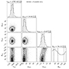 |
Fig. 8. Corner plot (Foreman-Mackey 2016) showing the posterior distributions of our simple kinematic model. The 16th, 50th, and 84th percentiles are indicated in the histograms with dashed lines. The kinematic angle is ill constrained due to the low velocity amplitude. |
With the larger sample of GCs, we do not find any indication of a rotating GCS as proposed by Lewis et al. (2020) who used the velocities from van Dokkum et al. (2018a) and van Dokkum et al. (2018b) in a very similar model as the one used here. However, when using their GC sample, we found comparable values for the rotation and dispersion as in Lewis et al. (2020), illustrating the effect small GC numbers combined with large velocity uncertainties can have. To test this further, we also ran the model using restricted GC samples containing only the MUSE GCs or only the FLAMES GCs, finding similar results. To test the influence of outliers (see Laporte et al. 2019), we randomly removed one or two GCs. However, the only GC that has a notable effect on the inferred velocity dispersion is GC101. Removing it, we find  km s−1. As NGC 1052-DF2 already has a relative radial velocity of +315 km s−1 compared to the NGC 1052 group (van Dokkum et al. 2022b), it is unlikely that this GC is an interloper from the group. However, it is possible that this GC is in the process of being stripped from the galaxy or that its measured velocity is not reliable. In our testing, we consistently measured its elevated velocity, but given the rather low S/N, it is possible that the fit converges on a noise feature and deeper data would be required to exclude this possibility (see Appendix A).
In summary, we find here a low velocity dispersion of the GCS that is comparable with previous estimates under consideration of the uncertainties. Also, the low dispersion of the GCs is comparable to the stellar velocity dispersion found from MUSE ( km s−1; Emsellem et al. 2019) or KCWI (
 km s−1; Danieli et al. 2019).
5. Discussion
In this work, we reanalysed the GCS in NGC 1052-DF2 using data from archival MUSE, with a focus on providing an updated view of their stellar populations and the GCS kinematics. In the following, we discuss our results in the context of previous studies.
5.1. Dynamical mass estimates
Connected to their measurements of the GCS velocity dispersion, several studies have estimated the dynamical or halo mass of NGC 1052-DF2 using different mass estimators of varying complexity. In the original work, van Dokkum et al. (2018a) used a tracer mass estimator that considers the individual GC velocities as well as their spatial distribution in a potential. For different assumptions of the velocity anisotropy and at a distance of 20 Mpc, they infer an upper limited of the total mass within 7.6 kpc of Mdyn < 3.4 × 10⁸ M⊙, while the stellar mass is estimated to be M* ∼ 2 × 10⁸ M⊙ (from LV = 1.1 × 10⁸ M⊙). This implied a dynamical mass-to-light ratio (Mdyn/LV) of order unity, therefore suggesting a lack of DM in this galaxy. Using a different approach to model the individual GC velocities from van Dokkum et al. (2018a), Martin et al. (2018) found  km s−1 and Mdyn < 3.7 × 10⁸ M⊙ within the effective radius (2.2 kpc = 22.7″; van Dokkum et al. 2018a), corresponding to Mdyn/LV < 6.7.
Also incorporating the velocity dispersion of the stars, Emsellem et al. (2019) derived dynamical mass estimates from different estimators that are proportional to Re σGCS2G−1 (Wolf et al. 2010; Amorisco & Evans 2011; Courteau et al. 2014; Errani et al. 2018). They found Mdyn/LV between ∼3.5 and 4.4 when assuming a distance of 20 Mpc, or Mdyn/LV between 5.8 and 6.0 when assuming a distance of 13 Mpc (Re = 1.4 kpc). In their rotation model, Lewis et al. (2020) find values of Mdyn/LV > 10 depending on the inclination of the system.
With a larger number of GCs and improved uncertainties, we provide here an updated dynamical mass estimate. Similar to Emsellem et al. (2019), we employed a simple estimator for the mass within 1.8 of the effective radius Mdyn(< 1.8Re) = 6.3 Re σGCS2G−1 (Errani et al. 2018). Assuming a distance of 16.2 Mpc (Re = 1.71 kpc), we find  and
and  for σGCS = 14.86 km s−1. At a larger distance of 20.0 Mpc, this would correspond to
  and
and  . Consequently, the higher velocity dispersion found here in combination with a smaller distance (Paper I), leads to a higher M/L and a higher dynamical mass than originally proposed.
However, in the case GC101 truly is an interloper or being stripped, σ is reduced to 8.63 km s−1 and consequently  and
and  . At the larger distance of 20 Mpc, the mass-to-light ratio would further decrease to
  . In this case, the mass-to-light ratio of the galaxy is low, irrespective of the distance.
The dynamical mass of a galaxy is known to follow a tight relation with the total number of GCs or the total GCS mass (e.g. Spitler & Forbes 2009; Harris et al. 2017; Forbes et al. 2018), suggesting that both the galaxy halo and the GCS were established during early stages of galaxy formation. With its remarkably bright GCs and low velocity dispersion, NGC 1052-DF2 was proposed to be an outlier of this relation (e.g. van Dokkum et al. 2018c). To test this, we place NGC 1052-DF2 on a plane showing dynamical masses versus GC numbers in Fig. 9. As comparison samples, we used the Local Group spheroidal dwarf galaxies from Forbes et al. (2018) and calculated their dynamical masses with the simple mass estimator from Errani et al. (2018). As a sample of more massive galaxies, we used galaxies in the Fornax cluster for which GCS velocity dispersions are available from Fahrion et al. (2020a) and GC numbers from Liu et al. (2019) and calculated their dynamical masses in the same fashion. Additionally, we used GC velocity dispersions and GC numbers complied by Gannon et al. (2024) for literature UDGs (in this case using data from Beasley et al. 2016; Toloba et al. 2018; Forbes et al. 2019; Lim et al. 2020; Gannon et al. 2020, 2021; Forbes et al. 2021; Danieli et al. 2022, and Toloba et al. 2023). Gannon et al. (2024) also included NGC 1052-DF2 in their catalogue, but we used here our updated measurements.
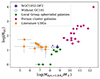 |
Fig. 9. Total number of GCs versus the dynamical mass estimate derived from the GCS velocity dispersion and the galaxy effective radius. NGC 1052-DF2 is shown in purple, Local Group dwarfs in green (data from Forbes et al. 2018), Fornax cluster galaxies in pink (data from Fahrion et al. 2020a and Liu et al. 2019), and literature UDGs in orange from the compilation by Gannon et al. (2024). The empty purple circle shows the dynamical mass estimate if GC101 is considered an interloper not belonging to the galaxy. |
As can be seen from this figure, the updated dynamical mass estimate places NGC 1052-DF2 among other similar galaxies (see also Trujillo et al. 2019), even with considering GC101 as an outlier. In particular, compared to other UDGs, NGC 1052-DF2 has a rather large dynamical mass as estimated from its GCs. Nonetheless, we note here again that the reported dynamical mass is just meant as a simple estimate based on the velocity dispersion of the GCS and the host galaxy effective radius. To infer from this the halo mass, the DM profile would need to be modelled (see e.g. Aditya 2024).
5.2. Globular cluster metallicities
The properties of the GCs in NGC 1052-DF2 have been discussed extensively, in particular with respect to their extreme luminosities and large sizes when a distance of D ∼ 20 Mpc is assumed (van Dokkum et al. 2018c; Shen et al. 2021b). Besides their bright magnitudes, van Dokkum et al. (2022a) found with an analysis of very deep HST ACS data that the bright GCs have a narrow colour range with a scatter of only ∼0.015 mag. The fainter (not spectroscopically confirmed) GCs analysed in their study appear to have a larger colour variation, but also larger uncertainties. Nevertheless, at first glance, the monochromatic nature of the GCs is in contrast to our finding of both metal-rich and metal-poor GCs. However, the GCs analysed in van Dokkum et al. (2022a) were from the spectroscopically confirmed GCs known at the time, while four of the five metal-rich GCs found here were not covered in that analysis. Additionally, as shown in Fig. 5, the colours reported by van Dokkum et al. (2022a) fall into the region where the CZR has a steep slope. Consequently, a narrow colour range does not imply a narrow range of metallicities.
While a broad distribution of GC metallicities is typically found in massive galaxies (e.g. Peng et al. 2006), dwarf galaxies in the Local Group are also known to host a rather large number of GCs with varying metallicities (see the compilation in Beasley et al. 2019). For example, NGC 185 (MV = −14.8 mag; McConnachie 2012) hosts GCs with metallicities between [M/H] = −2.0 and −0.5 dex, while NGC 205 (MV = −14.6 dex) has GCs with metallicities from [M/H] = −1.2 to −0.5 dex (Sharina et al. 2006). Both galaxies have similar luminosities as NGC 1052-DF2 (MV = −14.9 mag from van Dokkum et al. 2018a at a distance of 16.2 Mpc) and also a substantial number of GCs, but have smaller effective radii (McConnachie 2012).
5.3. Implications for the formation of NGC 1052-DF2
Given the initial observed low DM fraction and luminous GCS, several mechanisms were discussed to explain NGC 1052-DF2’s properties and formation history. For example, an origin as an old tidal dwarf galaxy that has formed from gas expelled from a massive galaxy undergoing tidal interactions (e.g. Mirabel et al. 1992; Bournaud & Duc 2006; Ploeckinger et al. 2018; Haslbauer et al. 2019) was discussed (e.g. van Dokkum et al. 2018a; Fensch et al. 2019). Assuming the closer distance of 16.2 Mpc combined with the our fiducial kinematic model, NGC 1052-DF2 does not appear to lack DM, as would be expected for a tidal dwarf galaxy. With GC101 as an outlier, the dynamical mass estimate is lower, but even then the old stellar age and low metallicity of NGC 1052-DF2 are at odds with the typically metal-rich and young populations found in tidal dwarfs (e.g. Weilbacher et al. 2003; Duc et al. 2014). As discussed by van Dokkum et al. (2018a) and Fensch et al. (2019), the old age and low metallicity would imply a formation at high redshift.
As an alternative scenario, tidal interactions with galaxies of the NGC 1052-DF2 group were suggested to have stripped the DM halo of NGC 1052-DF2 (e.g. Macciò et al. 2021). However, the closer distance would place NGC 1052-DF2 in front of the NGC 1052 group. Additionally, recent deep imaging of NGC 1052-DF2 has shown no evidence of tidal interactions down to μg = 30.9 mag arcsec−2 (Golini et al. 2024). In contrast, the same study found tidal tails around NGC 1052-DF4, another galaxy with a very low GCS velocity dispersion that has also been proposed to lack DM (van Dokkum et al. 2019). Nonetheless, as any stripping will always affect the DM first (e.g. see the discussions in Montes et al. 2020, Smith et al. 2015, and Smith et al. 2016), the low mass-to-light ratio found in the case GC101 is considered as an interloper together with the otherwise ordinary GC and stellar populations of NGC 1052-DF2 could be an indication of an incomplete stripping. Additionally, the higher velocity of GC101 might be explained if this GC is in the process of being stripped.
To explain the properties and spatial configuration of both NGC 1052-DF2 and NGC 1052-DF4, van Dokkum et al. (2022b) proposed a ‘bullet dwarf’ collision scenario, in which the two UDGs were formed as a result of two gas-rich progenitor galaxies colliding (see also Silk 2019; Lee et al. 2024). Reminiscent of the bullet galaxy cluster (e.g. Clowe et al. 2004, 2006), the DM haloes get separated from the gas in the collision. As one consequence of this scenario, GCs are expected to form in a single event from the available gas and therefore should all have a single metallicity. In contrast, our finding of a range of GC metallicities instead implies different episodes of GC formation, through either continuous formation and enrichment of GCs at high redshifts or assembly through the mergers of subsystems as discussed for more massive galaxies (e.g. Zepf & Ashman 1993; Beasley 2020). For this reason, if NGC 1052-DF2 formed in such a scenario, at least some of the GCs were either already present or formed after the event (see also the discussion in van Dokkum et al. 2022a). Also, it is unclear if a distance of 16.2 Mpc can be reconciled with this scenario.
Trujillo-Gomez et al. (2021) proposed a major merger origin of NGC 1052-DF2 to explain the formation of its luminous GCS. While a lower distance to the galaxy results in a more ordinary GC mass function (see Fig. 6), a gas-rich merger might still have triggered star and cluster formation and could explain the range of GC metallicities if the some GCs were accreted in the merger while others were newly formed. The old GC ages place such a merger at high redshift, but the age uncertainties are unfortunately too large to constrain which GCs might have formed in such a merger.
If placed at 16.2 Mpc, many properties of NGC 1052-DF2 are in line with Local Group dwarf galaxies, including its dynamical mass, GC number, GC mass function and the range of GC metallicities. However, it remains more extended than typical dwarf galaxies and still falls into the UDG category. Considering GC101 as an outlier, its dynamical mass also becomes rather low. While our study does not allow us to exactly determine the formation history of NGC 1052-DF2, it is possible that this galaxy is simply located in the tail of the size distribution of dwarf galaxies, or perhaps its stellar body has expanded. In general, several mechanisms have been proposed to explain the large sizes of UDGs, including external effects such as tidal interactions or ram pressure stripping (e.g. Carleton et al. 2019; Sales et al. 2020), internal feedback (e.g. Di Cintio et al. 2017; Chan et al. 2018), or formation in high-spin haloes (e.g. Amorisco & Loeb 2016; Liao et al. 2019). Using simulations, Benavides et al. (2024) recently showed that flat metallicity gradients in UDGs like the one found in NGC 1052-DF2 are not expected from gradual evolution in high-spin haloes, but might rather be an effect of outflows from star formation or stripping. Similarly, also the NIHAO simulations found flat (or negative) gradients in UDGs formed via supernovae feedback (Cardona-Barrero et al. 2023). Consequently, the flat stellar population gradients in NGC 1052-DF2 together with the GC metallicity distribution might suggest that this galaxy has started out as a rather regular galaxy that has expanded due to feedback from intense star formation.
6. Conclusions
This paper presents an updated view of the GCS of NGC 1052-DF2. Using archival MUSE IFS data, we extracted the spectra of 12 GC candidates. We established the membership of 11 of them, including 4 GCs that have not yet been confirmed. Together4 with newly acquired high-resolution FLAMES spectra of 10 GCs, the number of spectroscopically confirmed GCs of NGC 1052-DF2 is increased to 16. Our results are summarised as follows:
-
Using full spectrum fitting, we determined the individual ages and metallicities of the GCs in the MUSE field of view. We find overall old ages (> 9 Gyr) and a range of metallicities from [M/H] = −0.73 dex to [M/H] = −1.86 dex. Uncertainties on the GC metallicities range from 0.08 to 0.24 dex.
-
Comparing GC metallicities with their colours, we find them to scatter on the CZR. Nonetheless, with their low metallicities (and blue colours), they fall in a region where the slope of the CZR is steep and hence a small colour difference can correspond to a range of GC metallicities.
-
We obtained radial profiles of the host stellar metallicity and ages, finding flat profiles within the uncertainties. Many of the GCs are more metal-poor than the host at the same position but have similarly old ages.
-
From the ages and metallicities, we then derived mass-to-light ratios using the predictions of the EMILES SSP models, finding values between 1.2 and 2.0 for the HST ACS F606W filter. By deriving photometric masses, we find that the GCS mass function peaks at ∼105.4 M⊙, which is in agreement with the canonical peak of the GC mass function and the Milky Way GC mass function.
-
We combined the GC velocities from MUSE with the high-precision velocities from FLAMES to build a simple kinematic model of the GCS using 16 GCs. We find a velocity dispersion of
 km s−1 and no indication of rotation in the GCS. The velocity dispersion is insensitive to outliers with the exception of GC101. Excluding this GC, which has a low S/N spectrum, the velocity dispersion is reduced to
  km s−1. Even if deeper data confirm the higher relative velocity of GC101, it could still be an interloper from the group or could be in the process of being stripped.
 -
From this dispersion, we estimate a dynamical mass of
 and
and  , similar to other dwarf galaxies with such a mass. Assuming GC101 is an interloper, we find
  and
and  . Comparing the dynamical mass estimates to similarly derived values for other galaxies, NGC 1502-DF2 does not appear as an outlier.
We find NGC 1052-DF2 to be an extended, low-mass galaxy with a rich GCS with a range of metallicities and a low dynamical mass. Its exact origin cannot be determined based on currently available data, but it is possible that it is a ‘puffed up’ dwarf galaxy with a likely complex formation history shaped by hierarchical assembly of smaller structures and internal feedback.
We note that the mismatch between EMILES SSP predictions and observed colours does not affect the age and metallicity measurements because the pPXF fitting uses polynomials that make the result insensitive to the overall colour.
Acknowledgments
We thank the anonymous referee for a constructive report that has helped to polish this manuscript. We thank Mireia Montes and Ignacio Trujillo for helpful comments. This project has received funding from the European Union’s Horizon Europe research and innovation programme under the Marie Skłodowska-Curie grant agreement No 101103830. KF acknowledges support through the ESA research fellowship programme. TJ acknowledges the MUNI Award in Science and Humanities MUNI/I/1762/2023. This work made use of Astropy: a community-developed core Python package and an ecosystem of tools and resources for astronomy (Astropy Collaboration 2013, 2018, 2022). Based on observations collected at the European Southern Observatory under ESO programmes 2101.B-5008(A) and 110.23P4.001.
References
- Aditya, K. 2024, A&A, 689, A161 [NASA ADS] [CrossRef] [EDP Sciences] [Google Scholar]
- Amorisco, N. C., & Evans, N. W. 2011, MNRAS, 411, 2118 [Google Scholar]
- Amorisco, N. C., & Loeb, A. 2016, MNRAS, 459, L51 [NASA ADS] [CrossRef] [Google Scholar]
- Astropy Collaboration (Robitaille, T. P., et al.) 2013, A&A, 558, A33 [NASA ADS] [CrossRef] [EDP Sciences] [Google Scholar]
- Astropy Collaboration (Price-Whelan, A. M., et al.) 2018, AJ, 156, 123 [Google Scholar]
- Astropy Collaboration (Price-Whelan, A. M., et al.) 2022, ApJ, 935, 167 [NASA ADS] [CrossRef] [Google Scholar]
- Bacon, R., Accardo, M., Adjali, L., et al. 2010, in Ground-based and Airborne Instrumentation for Astronomy III, eds. I. S. McLean, S. K. Ramsay, & H. Takami, SPIE Conf. Ser., 7735, 773508 [Google Scholar]
- Bacon, R., Piqueras, L., Conseil, S., Richard, J., & Shepherd, M. 2016, Astrophysics Source Code Library [record ascl:1611.003] [Google Scholar]
- Baumgardt, H., & Hilker, M. 2018, MNRAS, 478, 1520 [Google Scholar]
- Beasley, M. A. 2020, in Reviews in Frontiers of Modern Astrophysics; From Space Debris to Cosmology, 245 [CrossRef] [Google Scholar]
- Beasley, M. A., Romanowsky, A. J., Pota, V., et al. 2016, ApJ, 819, L20 [NASA ADS] [CrossRef] [Google Scholar]
- Beasley, M. A., Leaman, R., Gallart, C., et al. 2019, MNRAS, 487, 1986 [Google Scholar]
- Beasley, M. A., Fahrion, K., & Gvozdenko, A. 2024, MNRAS, 527, 5767 [Google Scholar]
- Beasley, M. A., Fahrion, K., Guerra Arencibia, S., Gvozdenko, A., & Montes, M. 2025, A&A, 697, A144 [NASA ADS] [CrossRef] [EDP Sciences] [Google Scholar]
- Benavides, J. A., Sales, L. V., Abadi, M. G., et al. 2024, ApJ, 977, 169 [NASA ADS] [CrossRef] [Google Scholar]
- Bournaud, F., & Duc, P. A. 2006, A&A, 456, 481 [NASA ADS] [CrossRef] [EDP Sciences] [Google Scholar]
- Bradley, L., Sipőcz, B., Robitaille, T., et al. 2023, https://doi.org/10.5281/zenodo.7946442 [Google Scholar]
- Brodie, J. P., & Strader, J. 2006, ARA&A, 44, 193 [Google Scholar]
- Cappellari, M. 2017, MNRAS, 466, 798 [Google Scholar]
- Cappellari, M. 2023, MNRAS, 526, 3273 [NASA ADS] [CrossRef] [Google Scholar]
- Cappellari, M., & Emsellem, E. 2004, PASP, 116, 138 [Google Scholar]
- Cardona-Barrero, S., Di Cintio, A., Battaglia, G., Macciò, A. V., & Taibi, S. 2023, MNRAS, 519, 1545 [Google Scholar]
- Carleton, T., Errani, R., Cooper, M., et al. 2019, MNRAS, 485, 382 [NASA ADS] [CrossRef] [Google Scholar]
- Chan, T. K., Kereš, D., Wetzel, A., et al. 2018, MNRAS, 478, 906 [NASA ADS] [CrossRef] [Google Scholar]
- Clowe, D., Gonzalez, A., & Markevitch, M. 2004, ApJ, 604, 596 [NASA ADS] [CrossRef] [Google Scholar]
- Clowe, D., Bradač, M., Gonzalez, A. H., et al. 2006, ApJ, 648, L109 [NASA ADS] [CrossRef] [Google Scholar]
- Coelho, P. R. T. 2014, MNRAS, 440, 1027 [Google Scholar]
- Conroy, C., & van Dokkum, P. 2012, ApJ, 747, 69 [Google Scholar]
- Conroy, C., Villaume, A., van Dokkum, P. G., & Lind, K. 2018, ApJ, 854, 139 [Google Scholar]
- Conselice, C. J., Gallagher, I., J. S., & Wyse, R. F. G. 2003, AJ, 125, 66 [CrossRef] [Google Scholar]
- Côté, P., McLaughlin, D. E., Hanes, D. A., et al. 2001, ApJ, 559, 828 [CrossRef] [Google Scholar]
- Courteau, S., Cappellari, M., de Jong, R. S., et al. 2014, Rev. Mod. Phys., 86, 47 [Google Scholar]
- Dalcanton, J. J., Spergel, D. N., Gunn, J. E., Schmidt, M., & Schneider, D. P. 1997, AJ, 114, 635 [Google Scholar]
- Danieli, S., van Dokkum, P., Conroy, C., Abraham, R., & Romanowsky, A. J. 2019, ApJ, 874, L12 [NASA ADS] [CrossRef] [Google Scholar]
- Danieli, S., van Dokkum, P., Trujillo-Gomez, S., et al. 2022, ApJ, 927, L28 [NASA ADS] [CrossRef] [Google Scholar]
- Di Cintio, A., Brook, C. B., Dutton, A. A., et al. 2017, MNRAS, 466, L1 [NASA ADS] [CrossRef] [Google Scholar]
- Duc, P.-A., Paudel, S., McDermid, R. M., et al. 2014, MNRAS, 440, 1458 [NASA ADS] [CrossRef] [Google Scholar]
- Emsellem, E., van der Burg, R. F. J., Fensch, J., et al. 2019, A&A, 625, A76 [NASA ADS] [CrossRef] [EDP Sciences] [Google Scholar]
- Errani, R., Peñarrubia, J., & Walker, M. G. 2018, MNRAS, 481, 5073 [CrossRef] [Google Scholar]
- Fahrion, K., Lyubenova, M., van de Ven, G., et al. 2019, A&A, 628, A92 [NASA ADS] [CrossRef] [EDP Sciences] [Google Scholar]
- Fahrion, K., Lyubenova, M., Hilker, M., et al. 2020a, A&A, 637, A26 [NASA ADS] [CrossRef] [EDP Sciences] [Google Scholar]
- Fahrion, K., Lyubenova, M., Hilker, M., et al. 2020b, A&A, 637, A27 [NASA ADS] [CrossRef] [EDP Sciences] [Google Scholar]
- Fahrion, K., Bulichi, T.-E., Hilker, M., et al. 2022, A&A, 667, A101 [NASA ADS] [CrossRef] [EDP Sciences] [Google Scholar]
- Fensch, J., van der Burg, R. F. J., Jeřábková, T., et al. 2019, A&A, 625, A77 [NASA ADS] [CrossRef] [EDP Sciences] [Google Scholar]
- Ferré-Mateu, A., Gannon, J. S., Forbes, D. A., et al. 2023, MNRAS, 526, 4735 [CrossRef] [Google Scholar]
- Ferré-Mateu, A., Gannon, J., Forbes, D. A., et al. 2025, A&A, 694, L6 [NASA ADS] [CrossRef] [EDP Sciences] [Google Scholar]
- Forbes, D. A., Read, J. I., Gieles, M., & Collins, M. L. M. 2018, MNRAS, 481, 5592 [NASA ADS] [CrossRef] [Google Scholar]
- Forbes, D. A., Gannon, J., Couch, W. J., et al. 2019, A&A, 626, A66 [NASA ADS] [CrossRef] [EDP Sciences] [Google Scholar]
- Forbes, D. A., Gannon, J. S., Romanowsky, A. J., et al. 2021, MNRAS, 500, 1279 [Google Scholar]
- Foreman-Mackey, D. 2016, J. Open Source Software, 1, 24 [NASA ADS] [CrossRef] [Google Scholar]
- Foreman-Mackey, D., Hogg, D. W., Lang, D., & Goodman, J. 2013, PASP, 125, 306 [Google Scholar]
- Gannon, J. S., Forbes, D. A., Romanowsky, A. J., et al. 2020, MNRAS, 495, 2582 [NASA ADS] [CrossRef] [Google Scholar]
- Gannon, J. S., Dullo, B. T., Forbes, D. A., et al. 2021, MNRAS, 502, 3144 [Google Scholar]
- Gannon, J. S., Ferré-Mateu, A., Forbes, D. A., et al. 2024, MNRAS, 531, 1856 [NASA ADS] [CrossRef] [Google Scholar]
- Golini, G., Montes, M., Carrasco, E. R., Román, J., & Trujillo, I. 2024, A&A, 684, A99 [NASA ADS] [CrossRef] [EDP Sciences] [Google Scholar]
- Guérou, A., Krajnović, D., Epinat, B., et al. 2017, A&A, 608, A5 [Google Scholar]
- Harris, W. E. 2010, ArXiv e-prints [arXiv:1012.3224] [Google Scholar]
- Harris, W. E., Blakeslee, J. P., & Harris, G. L. H. 2017, ApJ, 836, 67 [Google Scholar]
- Hartman, K., Harris, W. E., Blakeslee, J. P., Ma, C.-P., & Greene, J. E. 2023, ApJ, 953, 154 [Google Scholar]
- Haslbauer, M., Dabringhausen, J., Kroupa, P., Javanmardi, B., & Banik, I. 2019, A&A, 626, A47 [NASA ADS] [CrossRef] [EDP Sciences] [Google Scholar]
- Impey, C., & Bothun, G. 1997, ARA&A, 35, 267 [NASA ADS] [CrossRef] [Google Scholar]
- Impey, C., Bothun, G., & Malin, D. 1988, ApJ, 330, 634 [Google Scholar]
- Iodice, E., Cantiello, M., Hilker, M., et al. 2020, A&A, 642, A48 [EDP Sciences] [Google Scholar]
- Iodice, E., Hilker, M., Doll, G., et al. 2023, A&A, 679, A69 [NASA ADS] [CrossRef] [EDP Sciences] [Google Scholar]
- Janssens, S., Abraham, R., Brodie, J., et al. 2017, ApJ, 839, L17 [NASA ADS] [CrossRef] [Google Scholar]
- Janssens, S. R., Forbes, D. A., Romanowsky, A. J., et al. 2024, MNRAS, 534, 783 [NASA ADS] [CrossRef] [Google Scholar]
- Jordán, A., McLaughlin, D. E., Côté, P., et al. 2007, ApJS, 171, 101 [CrossRef] [Google Scholar]
- Karachentsev, I. D., Karachentseva, V. E., Suchkov, A. A., & Grebel, E. K. 2000, A&AS, 145, 415 [NASA ADS] [CrossRef] [EDP Sciences] [Google Scholar]
- Laporte, C. F. P., Agnello, A., & Navarro, J. F. 2019, MNRAS, 484, 245 [NASA ADS] [CrossRef] [Google Scholar]
- Lee, J., Shin, E.-J., Kim, J.-H., Shapiro, P. R., & Chung, E. 2024, ApJ, 966, 72 [NASA ADS] [CrossRef] [Google Scholar]
- Lewis, G. F., Brewer, B. J., & Wan, Z. 2020, MNRAS, 491, L1 [NASA ADS] [CrossRef] [Google Scholar]
- Liao, S., Gao, L., Frenk, C. S., et al. 2019, MNRAS, 490, 5182 [NASA ADS] [CrossRef] [Google Scholar]
- Lim, S., Côté, P., Peng, E. W., et al. 2020, ApJ, 899, 69 [CrossRef] [Google Scholar]
- Liu, Y., Peng, E. W., Jordán, A., et al. 2019, ApJ, 875, 156 [NASA ADS] [CrossRef] [Google Scholar]
- Macciò, A. V., Prats, D. H., Dixon, K. L., et al. 2021, MNRAS, 501, 693 [Google Scholar]
- Martin, N. F., Collins, M. L. M., Longeard, N., & Tollerud, E. 2018, ApJ, 859, L5 [NASA ADS] [CrossRef] [Google Scholar]
- McConnachie, A. W. 2012, AJ, 144, 4 [Google Scholar]
- Mirabel, I. F., Dottori, H., & Lutz, D. 1992, A&A, 256, L19 [NASA ADS] [Google Scholar]
- Montes, M., Infante-Sainz, R., Madrigal-Aguado, A., et al. 2020, ApJ, 904, 114 [Google Scholar]
- Peng, E. W., Jordán, A., Côté, P., et al. 2006, ApJ, 639, 95 [Google Scholar]
- Pietrinferni, A., Cassisi, S., Salaris, M., & Castelli, F. 2004, ApJ, 612, 168 [Google Scholar]
- Pietrinferni, A., Cassisi, S., Salaris, M., & Castelli, F. 2006, ApJ, 642, 797 [Google Scholar]
- Ploeckinger, S., Sharma, K., Schaye, J., et al. 2018, MNRAS, 474, 580 [Google Scholar]
- Prole, D. J., van der Burg, R. F. J., Hilker, M., & Davies, J. I. 2019, MNRAS, 488, 2143 [NASA ADS] [Google Scholar]
- Ruiz-Lara, T., Trujillo, I., Beasley, M. A., et al. 2019, MNRAS, 486, 5670 [NASA ADS] [CrossRef] [Google Scholar]
- Sales, L. V., Navarro, J. F., Peñafiel, L., et al. 2020, MNRAS, 494, 1848 [Google Scholar]
- Sandage, A., & Binggeli, B. 1984, AJ, 89, 919 [Google Scholar]
- Sharina, M. E., Afanasiev, V. L., & Puzia, T. H. 2006, MNRAS, 372, 1259 [NASA ADS] [CrossRef] [Google Scholar]
- Shen, Z., Danieli, S., van Dokkum, P., et al. 2021a, ApJ, 914, L12 [NASA ADS] [CrossRef] [Google Scholar]
- Shen, Z., van Dokkum, P., & Danieli, S. 2021b, ApJ, 909, 179 [CrossRef] [Google Scholar]
- Shen, Z., van Dokkum, P., & Danieli, S. 2023, ApJ, 957, 6 [NASA ADS] [CrossRef] [Google Scholar]
- Silk, J. 2019, MNRAS, 488, L24 [NASA ADS] [CrossRef] [Google Scholar]
- Smith, R., Sánchez-Janssen, R., Beasley, M. A., et al. 2015, MNRAS, 454, 2502 [Google Scholar]
- Smith, R., Choi, H., Lee, J., et al. 2016, ApJ, 833, 109 [NASA ADS] [CrossRef] [Google Scholar]
- Soto, K. T., Lilly, S. J., Bacon, R., Richard, J., & Conseil, S. 2016, MNRAS, 458, 3210 [Google Scholar]
- Spitler, L. R., & Forbes, D. A. 2009, MNRAS, 392, L1 [Google Scholar]
- STScI Development Team 2018, Astrophysics Source Code Library [record ascl:1811.001] [Google Scholar]
- Taibi, S., Battaglia, G., Leaman, R., et al. 2022, A&A, 665, A92 [NASA ADS] [CrossRef] [EDP Sciences] [Google Scholar]
- Tang, Y., Romanowsky, A. J., van Dokkum, P. G., et al. 2025, ApJ, 978, 21 [NASA ADS] [CrossRef] [Google Scholar]
- Toloba, E., Lim, S., Peng, E., et al. 2018, ApJ, 856, L31 [CrossRef] [Google Scholar]
- Toloba, E., Sales, L. V., Lim, S., et al. 2023, ApJ, 951, 77 [NASA ADS] [CrossRef] [Google Scholar]
- Trujillo, I., Beasley, M. A., Borlaff, A., et al. 2019, MNRAS, 486, 1192 [Google Scholar]
- Trujillo-Gomez, S., Kruijssen, J. M. D., Keller, B. W., & Reina-Campos, M. 2021, MNRAS, 506, 4841 [NASA ADS] [CrossRef] [Google Scholar]
- Usher, C., Forbes, D. A., Brodie, J. P., et al. 2015, MNRAS, 446, 369 [NASA ADS] [CrossRef] [Google Scholar]
- van Dokkum, P. G., Abraham, R., Merritt, A., et al. 2015, ApJ, 798, L45 [NASA ADS] [CrossRef] [Google Scholar]
- van Dokkum, P., Danieli, S., Cohen, Y., et al. 2018a, Nature, 555, 629 [Google Scholar]
- van Dokkum, P., Cohen, Y., Danieli, S., et al. 2018b, Res. Notes Am. Astron. Soc., 2, 54 [Google Scholar]
- van Dokkum, P., Cohen, Y., Danieli, S., et al. 2018c, ApJ, 856, L30 [NASA ADS] [CrossRef] [Google Scholar]
- van Dokkum, P., Danieli, S., Cohen, Y., Romanowsky, A. J., & Conroy, C. 2018d, ApJ, 864, L18 [NASA ADS] [CrossRef] [Google Scholar]
- van Dokkum, P., Danieli, S., Abraham, R., Conroy, C., & Romanowsky, A. J. 2019, ApJ, 874, L5 [Google Scholar]
- van Dokkum, P., Shen, Z., Romanowsky, A. J., et al. 2022a, ApJ, 940, L9 [NASA ADS] [Google Scholar]
- van Dokkum, P., Shen, Z., Keim, M. A., et al. 2022b, Nature, 605, 435 [NASA ADS] [CrossRef] [Google Scholar]
- Vazdekis, A., Casuso, E., Peletier, R. F., & Beckman, J. E. 1996, ApJS, 106, 307 [Google Scholar]
- Vazdekis, A., Sánchez-Blázquez, P., Falcón-Barroso, J., et al. 2010, MNRAS, 404, 1639 [NASA ADS] [Google Scholar]
- Vazdekis, A., Koleva, M., Ricciardelli, E., Röck, B., & Falcón-Barroso, J. 2016, MNRAS, 463, 3409 [Google Scholar]
- Veljanoski, J., & Helmi, A. 2016, A&A, 592, A55 [NASA ADS] [CrossRef] [EDP Sciences] [Google Scholar]
- Villaume, A., Romanowsky, A. J., Brodie, J., et al. 2022, ApJ, 924, 32 [Google Scholar]
- Weilbacher, P. M., Duc, P. A., & Fritze-v Alvensleben, U. 2003, A&A, 397, 545 [NASA ADS] [CrossRef] [EDP Sciences] [Google Scholar]
- Wolf, J., Martinez, G. D., Bullock, J. S., et al. 2010, MNRAS, 406, 1220 [NASA ADS] [Google Scholar]
- Zaritsky, D., Donnerstein, R., Dey, A., et al. 2019, ApJS, 240, 1 [Google Scholar]
- Zaritsky, D., Donnerstein, R., Dey, A., et al. 2023, ApJS, 267, 27 [NASA ADS] [CrossRef] [Google Scholar]
- Zepf, S. E., & Ashman, K. M. 1993, MNRAS, 264, 611 [Google Scholar]
Appendix A: Fitting GC101
We show the fit to the FLAMES spectrum of GC101 in Fig. A.1. The shown fit is using the stellar population models from Coelho (2014), similarly as was used to fit the other FLAMES spectra as described in Paper I. To test the robustness of the fit, we tested different starting velocities for the PPXF call, wavelength ranges and templates, consistently finding the elevated radial velocity. However, as the figure shows, the spectrum is noisy with a S/N ≈ 5 pix−1, whereas the other GCs observed with FLAMES have S/N between 6 and 19 pix−1 (see Paper I). We can therefore not exclude systematic effects influencing the fit and deeper data would be needed to test this measurement.
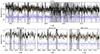 |
Fig. A.1. Full spectrum fit to the FLAMES spectrum of GC101. The original spectrum is shown in black, and the best-fit model is shown in orange. Shaded areas indicate masked regions due to sky line residuals. The lower panels show zoomed-in views around the calcium triplet lines. |
All Tables
All Figures
|
Fig. 1. RGB image of NGC 1052-DF2 created from the MUSE data. GCs analysed in this work are marked and labelled. Red: V, green: R, blue: I. See also Fensch et al. (2019). |
| In the text | |
|
Fig. 2. Full spectrum fitting of the GCs. Each panel shows the GC spectrum in black and the pPXF fit in orange. The respective residuals are shown in purple, shifted for visualisation. Grey shaded areas are regions masked from the fit due to sky residual or telluric lines. In the lower right corner, the best-fitting velocity is shown. The panels only show the blue part of the spectrum. |
| In the text | |
|
Fig. 3. Comparison of velocity measurements. Left: Comparison of GC velocities from this work based on the MUSE data and from the FLAMES spectra presented in Paper I. Middle: Comparison between this work and GC velocities from the same data as presented in Emsellem et al. (2019). Right: Comparison to GC velocities reported in van Dokkum et al. (2018a,b) from Keck DEIMOS and LRIS spectra. The dashed line shows the one-to-one relation, while the dotted line in the rightmost panel refers to a velocity offset of 12 km s−1 (see also Emsellem et al. 2019). |
| In the text | |
|
Fig. 4. Age versus metallicity of the GCs. Coloured dots refer to the MUSE GCs analysed here. The red cross shows the result from the stacked GC spectrum of Fensch et al. (2019), and the blue cross refers to the UDG itself as determined from an aperture spectrum. The dark red point shows the result from the stacked Keck spectra from van Dokkum et al. (2018c), and the green triangle shows the UDG metallicity from slit spectroscopy presented by Ruiz-Lara et al. (2019). |
| In the text | |
|
Fig. 5. CZR of the GCs. Each panel shows the spectroscopic metallicities versus HST F606W − F814W colour and predictions from the EMILES models colour-coded by age. From left to right: Colours from Paper I, Trujillo et al. (2019), van Dokkum et al. (2022a), and synthetic colours derived from the MUSE spectra directly. In the right panel, we also include the Fornax3D GC sample from Fahrion et al. (2020a). |
| In the text | |
|
Fig. 6. Distribution of derived masses based on stellar population properties. The orange histogram shows the NGC 1052-DF2 GCs assuming a distance of 16.2 Mpc, and the orange line shows a kernel density estimation line to visualise the distribution. We note that the histogram only shows the spectroscopically confirmed GCs and that no completeness correction was applied. The purple histogram and corresponding dotted purple line shows the mass distribution assuming a larger distance of 21.7 Mpc. The grey histogram and the black line show the distribution of 112 GCs from the Milky Way from Baumgardt & Hilker (2018). |
| In the text | |
|
Fig. 7. Radial metallicity and age profiles. Top: Metallicity profile of the stellar light obtained from elliptical annuli spectra in blue and GC metallicities in black. Bottom: Age profile for the stars and the GCs. |
| In the text | |
|
Fig. 8. Corner plot (Foreman-Mackey 2016) showing the posterior distributions of our simple kinematic model. The 16th, 50th, and 84th percentiles are indicated in the histograms with dashed lines. The kinematic angle is ill constrained due to the low velocity amplitude. |
| In the text | |
|
Fig. 9. Total number of GCs versus the dynamical mass estimate derived from the GCS velocity dispersion and the galaxy effective radius. NGC 1052-DF2 is shown in purple, Local Group dwarfs in green (data from Forbes et al. 2018), Fornax cluster galaxies in pink (data from Fahrion et al. 2020a and Liu et al. 2019), and literature UDGs in orange from the compilation by Gannon et al. (2024). The empty purple circle shows the dynamical mass estimate if GC101 is considered an interloper not belonging to the galaxy. |
| In the text | |
|
Fig. A.1. Full spectrum fit to the FLAMES spectrum of GC101. The original spectrum is shown in black, and the best-fit model is shown in orange. Shaded areas indicate masked regions due to sky line residuals. The lower panels show zoomed-in views around the calcium triplet lines. |
| In the text | |
Current usage metrics show cumulative count of Article Views (full-text article views including HTML views, PDF and ePub downloads, according to the available data) and Abstracts Views on Vision4Press platform.
Data correspond to usage on the plateform after 2015. The current usage metrics is available 48-96 hours after online publication and is updated daily on week days.
Initial download of the metrics may take a while.