| Issue |
A&A
Volume 697, May 2025
|
|
|---|---|---|
| Article Number | A22 | |
| Number of page(s) | 14 | |
| Section | Extragalactic astronomy | |
| DOI | https://doi.org/10.1051/0004-6361/202452271 | |
| Published online | 05 May 2025 | |
Quantifying observational projection effects with a simulation-based hot CGM model
1
Max Planck Institute for Extraterrestrial Physics (MPE), Gießenbachstraße 1, 85748 Garching, Munich, Germany
2
INAF-Osservatorio Astronomico di Brera, Via E. Bianchi 46, I-23807 Merate (LC), Italy
3
Smithsonian Astrophysical Observatory, Observatory Building E, 60 Garden St, Cambridge, MA 02138, USA
4
European Southern Observatory, Karl-Schwarzschild-Straße 2, 85748 Garching, Munich, Germany
5
Universitäts-Sternwarte München, Scheinerstraße 1, 81679 München, Germany
6
Max Planck Institute for Astrophysics, Karl-Schwarzschild-Straße 1, 85748 Garching, Munich, Germany
7
University of Geneva, 1205 Geneva, Switzerland
8
Institute for Computational Cosmology, Department of Physics, Durham University, South Road, Durham DH1 3LE, United Kingdom
⋆ Corresponding author: This email address is being protected from spambots. You need JavaScript enabled to view it.
Received:
17
September
2024
Accepted:
27
March
2025
Abstract
Aims. The hot phase of the circumgalactic medium (CGM) allows us to probe the inflow and outflow of gas responsible for dictating the evolution of a galaxy's structure. Studying the hot CGM sheds light on the physical properties of the gas phase of the baryons, which is crucial to inform and constrain simulation models. With the recent advances in observational measurements probing the hot CGM in X-rays and thermal Sunyaev-Zeldovich (tSZ), we have a new avenue for widening our knowledge of gas physics and feedback.
Methods. In this paper, we use the TNG300 hydrodynamical simulations to build a fully self-consistent forward model for the hot CGM. In order to do that, we construct a lightcone and generate mock X-ray observations of the large-scale structure. We quantify the main projection effects impacting CGM measurements, namely the locally correlated large-scale structure in X-rays and the effect due to satellite galaxies misclassified as centrals, which affect the measured hot CGM galactocentric profiles in stacking experiments.
Results. We present an analytical model that describes the intrinsic X-ray surface brightness profiles of halos across the stellar and halo mass bins. The increasing stellar mass bins result in decreasing values of β, the exponent quantifying the slope of the intrinsic galactocentric profiles. We measure the effect of misclassified centrals in stacking experiments for three stellar mass bins 1010.5−11 M⊙, 1011−11.25 M⊙, and 1011.25−11.5 M⊙. We find that the contaminating effect of the misclassified centrals on the stacked profiles increases when the stellar mass decreases. When stacking galaxies of Milky-Way-like stellar mass, this effect is dominant already at a low level of contamination: in particular, misclassified centrals contributing 30%, 10%, or 1% of a sample dominate the measured surface brightness profile at radii ≥0.11×R500c, ≥0.24×R500c, and ≥1.04×R500c, respectively.
Key words: galaxies: evolution / X-rays: galaxies
© The Authors 2025
 Open Access article, published by EDP Sciences, under the terms of the Creative Commons Attribution License (https://creativecommons.org/licenses/by/4.0), which permits unrestricted use, distribution, and reproduction in any medium, provided the original work is properly cited.
This article is published in open access under the Subscribe-to-Open model.
Open access funding provided by Max Planck Society.
1. Introduction
The circumgalactic medium (CGM) plays a crucial role in interfacing the gas between the interstellar medium (ISM) within galaxies and the external intergalactic medium (IGM) outside them. The CGM is commonly defined as the gas within the virial radii of the galaxy and outside their stellar disks. It is the gravitationally bound gas that encompasses the fossil imprints of the physical mechanisms, such as outflows, inflows, and feedback processes, dictating the evolution of the galaxy (see Tumlinson et al. 2017 for a review). These mechanisms are sensitive to the galaxy's environment and its halo properties, as shown by the complex Stellar-to-Halo-Mass-Relation (SHMR); see the review from Wechsler & Tinker (2018). According to most models, the SHMR indicates that the low-halo-mass end is sensitive to stellar and supernovae (SN) driven feedback (Dekel & Woo 2003; Benson et al. 2003), causing heating of the gas, hot bubbles (McKee & Ostriker 1977), galactic wind outflows (Dekel & Silk 1986), and turbulence (Ostriker & Shetty 2011; Strickland & Heckman 2009). In contrast, Active Galactic Nuclei (AGN) should be the main drivers of feedback in the high-halo-mass end (Silk & Rees 1998; Fabian 2012; Eckert et al. 2021). Of particular interest is the peak of the SHMR relation at the pivotal halo mass Mh∼1012 M⊙, similar to our Milky-Way (MW) mass, corresponding to the mass scale where star formation efficiency reaches its maximum. Thus, studying the volume-filling hot gas component of the CGM, especially in the MW halo mass regime, encapsulating a range of physical processes, is crucial for testing galaxy formation models (Faucher-Giguère & Oh 2023).
The most general scenario for the presence of such hot CGM assumes that infalling gas within halos ≳1012 M⊙ is shock heated up to the virial temperature, Tvir≳106 K, resulting in X-ray emission (White & Rees 1978). This hot gas is probed with the thermal Sunyaev-Zeldovich (Sunyaev & Zeldovich 1972, tSZ) effect at mm-wavelengths (Lim et al. 2021; Das et al. 2023; Oren et al. 2024) and in X-rays via absorption and emission. X-ray absorption studies use sightlines with bright background sources to probe the hot CGM via absorption lines like OVI or OVII Kα (Galeazzi et al. 2007; Bhattacharyya et al. 2023; Mathur et al. 2023). The major challenge in this technique is constructing statistical samples and mapping the large-scale extent of the CGM, which will improve with future X-ray telescopes with microcalorimeters (Wijers et al. 2020; Bogdán et al. 2023). On the emission side, studies use narrow-band and broad-band observations. The narrow-band emission comprising of OVII and OVIII metal lines dominates the lower halo mass regime 1012−1013 M⊙ (Bertone et al. 2010; van de Voort 2013; Wijers 2022) and is well-studied within our MW (Zheng et al. 2024; Locatelli et al. 2024; Ponti et al. 2023; Koutroumpa et al. 2007). However, for extragalactic studies, future high-spectral resolution instruments are required to distinguish the extragalactic emission from that of the MW foreground (Nelson et al. 2023; Truong et al. 2023; Schellenberger et al. 2024; ZuHone et al. 2024).
Multiple extragalactic single-object broad-band X-ray emission studies have been published (Bogdán et al. 2013a,b; Anderson et al. 2016; Bogdán et al. 2017; Li et al. 2017; Das et al. 2019). However, due to the X-ray emissivity scaling with the square of the density, detections are limited to the densest parts of the CGM, within 40−150 kpc from the galaxy centre. To map the extended CGM out to the halo virial radius, Rvir, Anderson et al. (2015) stacked SDSS galaxies with the full-sky X-ray data from the ROSAT survey. With the advent of SRG/eROSITA, we have unprecedented statistics for studying the hot CGM in X-rays with stacking analysis, as first shown by Oppenheimer et al. (2020), who generated mock observations with IllustrisTNG and EAGLE hydrodynamical simulations. Comparat et al. (2022) and Chadayammuri et al. (2022), and more recently, Zhang et al. (2024, hereafter Z+24) conduct such experiments with the eROSITA data and detect the hot CGM out to the virial radius of Milky-Way and M31-like galaxies. X-ray stacking analysis provides the most sensitive state-of-the-art observations of the hot CGM in the current observational landscape. Still, they are subject to various observational effects that affect the interpretation of the hot CGM. Consequently, we need a complete theoretical framework for describing the intrinsic hot CGM emission to disentangle the intrinsic signal from other observational effects.
A plethora of theoretical models (e.g., Faerman et al. 2017; Voit et al. 2019; Choudhury et al. 2019; Stern et al. 2024; Singh et al. 2021; Pandya et al. 2023; Faerman & Werk 2023) have been used to describe and predict the intrinsic properties of the hot CGM; Singh et al. (2024) discuss the comparison of some idealised cases. Similarly, Oppenheimer et al. (2020), Vladutescu-Zopp et al. (2025) made explicit predictions of the intrinsic hot CGM profiles obtained by assigning mock X-ray emission to the hot halos found in cosmological hydrodynamical simulations. However, before testing theoretical and numerical predictions of the hot CGM against state-of-the-art observations, we must quantify all the effects that influence the hot CGM observations in stacking experiments. Among the primary sources of contamination in X-ray stacking experiments, inhibiting us from retrieving the physical properties of the detected CGM emission, are (1) the unresolved AGN and X-ray binaries (XRB) population of galaxies (Biffi et al. 2018; Vladutescu-Zopp et al. 2023), and (2) the projection effects within the hot gas emission of the cosmic web. These projection effects include the contribution from the Large-Scale Structure (LSS) halo environment (locally correlated X-ray emission), the effect of satellite galaxies being misclassified as central due to limitations in the (photometric) redshift accuracy for the galaxies in large surveys (see, e.g., Weng et al. 2024), the offset between the X-ray centre and the centre defined by the minimum of the halo potential, and the Line-of sight (LoS) projection of uncorrelated X-ray emission of fore- and background structures. Z+24 tried to model these effects empirically for the first time; however, we need forward models based on cosmological hydrodynamical simulations for a complete description and full understanding of these contaminating effects.
In this paper, we analyse numerical simulations to empirically quantify the effects of the locally correlated X-ray emission and the misclassified centrals, also called the satellite-boost effect, relevant for measuring the hot CGM in stacking experiments. To do this, we use the TNG300 hydrodynamical simulations (Pillepich et al. 2018a; Marinacci et al. 2018; Naiman et al. 2018; Nelson et al. 2015; Springel et al. 2018) to construct a lightcone and generate mock X-ray observations. We focus here on the projection effects of hot gas affecting the X-ray surface brightness profiles. The structure of the paper is as follows. Section 2 details the construction of the TNG300 lightcone (LC-TNG300) used for modelling the hot CGM in this study. We explain all the projection effects in detail in Sect. 3. In Sect. 4, we describe the process for generating mock X-ray observations that mimic observational data and provide the machinery for computing the surface brightness profiles. Section 5 presents the main results of this work done with the TNG300 lightcone. Lastly, Sect. 6 discusses the main findings and Sect. 7 provides an overview with prospects.
2. Simulated lightcone with IllustrisTNG: LC-TNG300
Since we are interested in studying the impact of the locally correlated X-ray emission within the LSS environment of the halo, we require a simulation that contains all the complexities introduced by feedback and cooling, which are imprinted in X-ray measurements. We also require a large box size to encompass the effects of the cosmological LSS itself. Therefore, we use cosmological hydrodynamical simulations that self-consistently predict the LSS and its impact on gas dynamics within a halo. We use the IllustrisTNG cosmological hydrodynamical simulation with the box of side length 302.6 Mpc (TNG300; Nelson et al. 2019)1. IllustrisTNG accounts for many physical processes, among which the most notable ones are star formation regulated by a subgrid ISM model (Springel & Hernquist 2003), metal enrichment (Naiman et al. 2018), radiative gas cooling, galactic wind outflows (Pillepich et al. 2018b), magnetic fields and diffuse radio emissions (Marinacci et al. 2018), supermassive black hole growth with Bondi accretion and mergers, thermal and kinetic modes for black hole feedback (Weinberger et al. 2018). IllustrisTNG also reproduces correlation functions and power spectra of particles and halos (Springel et al. 2018). TNG300 contains 25003 dark matter particles, with a baryonic mass resolution of 1.1×10⁷ M⊙, a comoving value of the adaptive gas gravitational softening length for gas cells of 370 comoving parsec, gravitational softening of the collisionless component of 1.48 kpc, and dark matter mass resolution of 5.9×10⁷ M⊙. The TNG simulations adopt the Ade et al. (2016) cosmological parameters, with the matter density parameter Ωm=Ωdm+Ωb = 0.3089, baryonic density parameter Ωb = 0.0486, Hubble constant H0 = 100 h km/s/Mpc with h = 0.6774, and ΩΛ = 0.6911.
The Friends-of-Friends (FoF) algorithm is applied to the dark matter particles with linking length b = 0.2 to obtain the halos. The subhalos are retrieved with subfind (Springel et al. 2001; Dolag et al. 2009), which detects gravitationally bound substructures that are equivalent to galaxies in observations. Additionally, subfind also classified the subhalos into centrals and satellites, where centrals are the most massive substructure within a distinct halo.
To model the hot gas emission in the redshift range 0.03≲z≲0.3, as done in observations (e.g. Comparat et al. 2022; Chadayammuri et al. 2022; Zhang et al. 2024), we need four boxes lined up behind each other to arrive at the comoving distance, dC(z = 0.3), of 1231 Mpc. For a full-sky lightcone going up to z = 0.3, we must replicate and stack 512 boxes; however, in this technique, the large-scale projection effects cannot be estimated properly; see Merson et al. (2013). Therefore, we box remap2 all snapshots into a configuration where the longest length of one of the sides is ∼4× the original length (Carlson & White 2010). This technique ensures that the new elongated box has a one-to-one remapping, remains volume-preserving, and keeps local structures intact. For a box whose original dimensions are normalized to (1, 1, 1), the unique solution for the transformed box sides is (4.1231, 0.7276, 0.3333), respectively. We remap the coordinates of particles (gas, dark matter, and stars) and the halo and their subhalo catalogues. There are 22 snapshots within the observationally motivated redshift range of 0.03≤z≤0.3. Therefore, we obtain 22 remapped particle cuboids and 22 remapped galaxy catalogue cuboids at redshift z<0.3. We define the observer's position as being at a corner of the smallest face. The opening angles for the observer are (θLC obs, ϕLC obs) = (10.16, 4.64) degrees. The area subtended on the sky for a given observer is 47.28 deg2. We illustrate the lightcone constructed with the box remap technique in Fig. 1. We also publically release LightGen, the code used for generating the lightcone in this work.
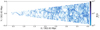 |
Fig. 1. Illustration of the lightcone built using TNG300 in the x−y plane. The figure shows the subhalos within LC-TNG300 at 0.03≤z≤0.3 remapped using boxremap (Carlson & White 2010). The observer is set at the (0, 0, 0) location. The lightcone goes out to 1231 cMpc along the x-axis, subtending an area of 47.28 deg2 on the sky in the y−z plane. The subhalos are colour-coded with their stellar masses. |
The distinct halos, CEN , and subhalos within the LC-TNG300 are catalogued with their physical properties and binned in stellar mass and halo mass bins, as shown in Table 1 and Table 2. We have 5, 109 centrals and 2, 719 satellites of stellar mass in the Milky Way range (M★ = 1010.5−11 M⊙), which is sufficient to statistically model the projection effects in these halos.
Stellar mass bins used to generate the X-ray surface brightness profiles.
Halo mass bins used to generate the X-ray surface brightness profiles.
This paper defines the stellar mass used from TNG300 as the mass within twice the stellar half-mass radius. We present quantities relative to both critical and mean densities because R500c3 is the radius most commonly used by X-ray astronomers (see e.g., Lyskova et al. 2023 and references therein), and R200m4 represents the halo's viral radius and is theoretically more relevant as it presents quantities within the virialized halo. The galaxy catalogue is divided into central, CENsim, and satellites, SATsim for the concerned stellar mass bins. To construct the SATsim catalogue, we refer to the halo/subhalo classification, where we match all the central galaxies with the distinct halos, thereby leaving behind all the secondary subhalos or satellites.
3. Contributions to observed X-ray surface brightness profiles
The main objective of this study is to model the various sources of contamination that come into play when measuring the hot gas component of the CGM. Here, we list all the components contributing to the observed X-ray surface brightness profile.
-
Intrinsic emission from the halo. This corresponds to the emission within the radius, R200m, of the central halo in 3D. We associate this X-ray emission with being intrinsic to the galaxy CGM. It must be noted that the definition of a halo boundary at which the gas is bound is non-trivial; we refer to Diemer et al. (2017) and references therein for more details.
-
Locally correlated environment. This component encapsulates the surrounding emission of the galaxy with the LSS in which it resides. Also known as the 2-halo term (Cooray & Sheth 2002; Kravtsov et al. 2004), this corresponds to the contribution arising due to the local background changing with the size of the halo. This effect is explored in tSZE studies, where Vikram et al. (2017), Lim et al. (2021) show the impact of the two-halo component, where the one-halo contribution at mass scales M200≤1013−13.5 h−1 M⊙ is swamped by the two-halo term due to nearby massive systems dominating the measured signal. Given our focus on MW-size halos, modelling the contribution from the locally-correlated background is crucial for disentangling intrinsic hot CGM emission from the local background.
-
Intrinsic emission from satellites. The X-ray emission from the satellite galaxy contributes to the total observed CGM emission in projection. As the host galaxy is more massive, with a deeper potential well, the contribution of this effect is negligible in stacking experiments (see Rohr et al. 2024 for further insights on the detectability of the satellite emission).
-
Contamination from misclassified centrals. In observations that use photometric surveys, classifications between centrals and satellites are inhibited due to limitations in the redshift accuracy. This effect is large and unavoidable for photometric surveys (∼30% contaminants for MW-like galaxies; Sect. 3.5 in Z+24) and significantly mitigated for spectroscopic surveys (∼1% contaminants for MW-like galaxies; Sect. 3.7 in Z+24), but not completely removed due to survey incompleteness or residual uncertainty in the central/satellite classification for systems with a low number of galaxies (see also Weng et al. 2024 who quantify the effect for absorbers in cold gas with TNG50). This implies that the measured X-ray surface brightness profiles in stacked samples of galaxies classified as centrals contain the intrinsic emission around truly central galaxies but are contaminated by the emission measured around satellites (off-centred) misclassified as centrals. In conclusion, including the emission around satellites in the stacking analysis alters the recovered profiles and, therefore, must be modelled.
-
The X-ray to true centre offset. The theoretically defined centre of a halo, which is the minimum of the dark matter potential well, could be offset from the observationally defined centres, e.g., the peak of the SZ signal or the X-ray emission, or the optical/infrared centre inferred from the stellar distribution (Zitrin et al. 2012; Lauer et al. 2014; Saro et al. 2015; Cui et al. 2016; Seppi et al. 2023). This offset is associated with physical effects such as galaxy mergers (Martel et al. 2014), misidentification of the brightest halo galaxy (Hoshino et al. 2015; Hikage et al. 2018; Oguri et al. 2018; Zhang et al. 2019) or failure of the brightest halo galaxy being a proxy for the minimum of the halo potential in optical studies (Skibba et al. 2011). Overall, miscentering causes a smoothing effect in stacking studies (Oguri & Takada 2011), and therefore, must be calibrated and modelled. This effect of miscentering correlates with halo mass; hence, it is well-studied at the cluster and group scales. As we simulate X-ray emission around lower mass, MW-like halos in this work, we extend the discussion of miscentering of the X-ray emission from the minimum of the host halo potential to MW mass scales (see discussion in Sect. 6.3).
-
Contamination from other X-ray sources. Other X-ray emitting sources like XRB and AGN contaminate the measured hot CGM. XRB emission is distributed on the scale of the stellar body of a galaxy; however, for an instrument with a point spread function (PSF) like eROSITA, it is unresolved and appears as a point source. Z+24 take special precautions to account for this by masking the eROSITA detected point sources within the X-ray data. They also model additional contributions from the unresolved XRB and AGN. For this study, we leave the modelling of the AGN and XRB resolved/unresolved emissions with the LC-TNG300 for future work.
-
Line of sight (LoS) projection. Objects along the line of sight, which do not reside near the galaxy, also contaminate the detected signal. Nevertheless, this uncorrelated contamination is well-modelled as the large-scale background and foreground in observations and, therefore, is not discussed further in this work.
-
Other X-ray background components. The local flat background is a combination of (1) the Soft X-ray background (SXRB; Henley & Shelton 2010, 2012, 2013; Nakashima et al. 2018; Gupta et al. 2023; Pan et al. 2024; Yeung et al. 2024), which is composed of emission from the local hot bubble, the MW CGM, other intervening galactic structure and the time variable solar-wind charge exchange, (2) the Cosmic X-ray background (De Luca & Molendi 2004; Gilli et al. 2007; Luo et al. 2016; Cappelluti et al. 2017), which is dominated by AGN, and (3) the instrumental effects. In this study, we simulate intrinsic X-ray events from hot gas alone; therefore, this study does not expand on the impacts of the other well-studied X-ray background components.
This work focuses on modelling the locally correlated environment and the effect due to misclassified-centrals (the satellite-boost effect). We also quantify the effect of the X-ray to true centre offset for the halo mass bins considered in this work.
4. Method
We detail the process to create mock X-ray observations in Sect. 4.1 and introduce the formalism used to fit the X-ray surface brightness profiles in Sect. 4.2. We detail the data products generated to study the projection effects in Sect. 4.3.
4.1. Mock X-ray observation
The photons are simulated in the 0.5−2.0 keV intrinsic band with pyXsim (ZuHone & Hallman 2016), which is based on phox (Biffi et al. 2013), by assuming an input emission model where the hot X-ray emitting gas is in collisional ionisation equilibrium. The spectral model computations of hot plasma use the Astrophysical Plasma Emission Code, apec5 code (Smith et al. 2001) with atomic data from atomdb v3.0.9 (Foster et al. 2012). This model requires the plasma temperature of the gas cells (in keV), the metal abundances, the redshift z and the normalisation,
![Mathematical equation: $$ N = \frac {10^{-14}}{4 \pi [D_{\rm A}(1+z)]^2} \int n_{\rm e} n_{\rm H} {\rm {d}V}, $$](/articles/aa/full_html/2025/05/aa52271-24/aa52271-24-eq10.gif) (1)
(1)
where DA is the angular diameter distance to the source (cm), dV is the volume element (cm3), ne and nH are the electron and hydrogen densities (cm−3), respectively. The temperature is calculated from the internal energy u and the electron abundance xe(=ne/nH) of the gas cells6. The temperature T for every gas cell is defined as
 (2)
(2)
where kB is Boltzmann's constant in CGS units and γ = 5/3 is the adiabatic index. The mean molecular weight μ is given as
 (3)
(3)
where XH = 0.76 is the hydrogen mass fraction and mp is the proton mass in grams. The metal abundances within TNG are provided for the snapshots at redshift intervals of every 0.1. As a result, 19 of the 22 snapshots within the lightcone constructed in this work lack metallicity information. Given the lack of metallicity information and the inaccuracies introduced by extrapolation of metallicity values between the 0.1 redshift intervals due to the evolution of gas particles, we assume a constant metallicity of 0.3 Z⊙; this is consistent with measurements for our MW (Miller & Bregman 2015; Bregman et al. 2018; Kaaret et al. 2020; Ponti et al. 2023). This work uses the solar abundance values from Anders & Grevesse (1989).
The TNG star formation model is based on the subgrid two-phase model proposed by Springel & Hernquist (2003), with some modifications (see Pillepich et al. 2018a, and references therein). The gas cells that emit efficiently in the soft X-ray band (i.e. [0.3–5] keV) are due to the SN-driven kinetic decoupled winds, which ultimately deposit energy into non-star-forming gas cells. Additionally, the hot component of this two-phase model exhibits typically high temperature (>105 K). As further explained in Truong et al. (2020) (see Appendices B–C), because this multiphase structure within the TNG model is not resolved, and it is instead modelled by a simplistic two-phase structure with unrealistic assumptions, we cannot make a sensible estimate of the X-ray emission from the unresolved phases of the ISM. Therefore, by excluding the parameter space of the warm-neutral ISM (Le Brun et al. 2014; Rahmati et al. 2016; Wijers et al. 2019), namely: (1) excluding star-forming gas cells, (2) ignoring gas cells below 105 K, and (3) ignoring gas cells with densities above 10−25 g/cm3, we ensure the gas particles used in this work are physically emitting X-rays.
Within pyXSim, the number of photons generated depends on the specified collecting area of the assumed X-ray telescope, its exposure time, and redshift. We generate sufficient photons by assuming a telescope with an energy-independent collecting area of 1000 cm2 (about 3/4 of the eROSITA field-of-view-average effective area at 1 keV) and an exposure time of 1000 ks. The photon-list is generated in the observed frame of the X-ray emitting gas cells and is corrected to rest frame energies. The LoS direction determines the event's position in the sky. We define the LoS along the x-axis within the lightcone. By applying a θLC obs/2 = 5.08 deg rotation along the z-axis and −ϕLC obs/2=−2.32 deg rotation along the y-axis, we centre the y−z plane at (0, 0) degrees. The photons generated by the gas particles are projected onto the sky; the resulting image is shown in Fig. 2.
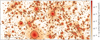 |
Fig. 2. Projected rest-frame X-ray events from the TNG300 ligthcone in the 0.5−2.0 keV band for a telescope with energy-independent collecting area 1000 cm2 and exposure time of 1000 ks. The events are generated using the hot gas cells within the TNG300 lightcone at redshifts 0.03−0.3 using pyXsim (ZuHone & Hallman 2016). The centre for the projection onto the sky is chosen as RA, Dec ≡ (0., 0.) degrees. The contours represent the two X-ray surface brightness levels of 5×10⁻¹⁴ erg s−1 cm−2 arcmin−2 and 2×10⁻¹⁶ erg s−1 cm−2 arcmin−2. |
We also project the halo and subhalo positions on the sky, as shown in Fig. 3 for a redshift slice of z = 0.3. The X-ray events are then stacked around the projected halo/subhalo positions. The surface brightness profiles7 are calculated 𝒮(r) as a function of the projected radius on the sky within the 0.5−2 keV energy band. The centre is chosen as the location of the most bound particle within the halo/subhalo as found by the FoF/subfind algorithm. The number of photons with rest frame energy E [erg] in each radially outward bin r, N(E, r), is weighted by the area, 𝒜 [kpc2], of the 2D shell between r and r+dr, the fraction of photons collected from the source, fA, and the exposure time, texp [seconds],
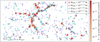 |
Fig. 3. Projected halos (centrals) are overplotted with their corresponding scaled R500c at z = 0.3; the R500c of the halos are represented by the size of the circles. We also show the projected rest-frame X-ray events from the TNG300 ligthcone in the 0.5−2.0 keV band for a telescope with energy-independent collecting area 1000 cm2 and exposure time of 1000 ks at the redshift slice of 0.284≤z≤0.3. The halos with M200m∈1014−14.5 M⊙ are shown in red, M200m∈1013.5−14 M⊙ in grey, M200m∈1013−13.5 M⊙ in cyan, and M200m∈1012.5−13 M⊙ in blue. |
![Mathematical equation: $$ {\cal {{S}}}_{\rm X}(r) = \frac {\sum _{E_i= 0.5\ {\rm keV}}^{2\ {\rm keV}}N(E_i, r)\ E_i}{f_{\rm A} t_{\rm exp} {\cal {{A}}}(r)}\ \Bigg [\frac {\rm erg}{\rm sec\ kpc^2}\Bigg ]. $$](/articles/aa/full_html/2025/05/aa52271-24/aa52271-24-eq13.gif) (4)
(4)
Here, fA is the fraction of the source photons collected by the synthesized telescope that has a collecting area A:
 (5)
(5)
where dL(z) is the luminosity distance to the source.
4.2. X-ray surface brightness profiles and their analytic modelling
The hot CGM surface brightness profile can be analytically described by the β model (Cavaliere & Fusco-Femiano 1976);
![Mathematical equation: $$ \bar {{\cal {{S}}}}_{\rm X, 0.5-2.0\ keV}[r] = S_0 \left [1 + \left (\frac {r}{r_{\rm c}} \right )^2 \right ]^{-3\beta + \frac {1}{2}}, $$](/articles/aa/full_html/2025/05/aa52271-24/aa52271-24-eq15.gif) (6)
(6)
where S0 is the central surface brightness, rc is the core radius at which the profile slope becomes steeper, and β is the exponent quantifying the slope of the profile. In cases where the outskirt steepens more than the slope defined for the inner radii by the β−model, following Vikhlinin et al. (2006), we introduce a new slope-parameter,
![Mathematical equation: $$ \bar {{\cal {{S}}}}_{\rm X, 0.5-2.0\ keV}[r] = S_0 \left [1 + \left (\frac {r}{r_{\rm c}} \right )^2 \right ]^{-3\beta + \frac {1}{2}} \times \left [1 + \left (\frac {r}{r_{\rm s}} \right )^\gamma \right ]^{-\epsilon /\gamma }, $$](/articles/aa/full_html/2025/05/aa52271-24/aa52271-24-eq16.gif) (7)
(7)
where rs is the scale radius at which the slope changes to ϵ and γ defines the width of the transition region. We fix γ = 3 and restrict the priors on rs>rc and ϵ<5, as suggested by Vikhlinin et al. (2006), in the fitting procedure.
4.3. Prerequisite data products for quantifying projection effects
To obtain contributions from the large-scale structure, the locally correlated X-ray emission, we generate cubes and profiles with the CENsim catalogue for the two cases as follows:
-
R200m cubes and profiles: every central galaxy within the halo catalogue is assigned X-ray events within R200m of the parent halo. We define these profiles as the intrinsic hot gas emission profiles.
-
R±3Mpc, R±9Mpc and R±27Mpc cubes and profiles: all the X-ray events, intrinsic and locally extrinsic, irrespective of whether they belong to the galaxy but within 3 Mpc, 9 Mpc, and 27 Mpc of the source centre, are selected in 3D spherical comoving volumes. We construct the profiles and cubes to quantify the impact of contamination from the local vicinity on the intrinsic source emission.
To quantify contributions from the emission associated with misclassified centrals, we use the SATsim catalogue in the same stellar mass bin as the central galaxies. For galaxies in the three stellar mass bins 1010.5−11 M⊙, 1011−11.25 M⊙, and 1011.25−11.5 M⊙, we construct a total galaxy samples containing Ntot galaxies, of which there are Ncen centrals and Nsat satellites. The number of satellites is defined as Nsat=fsatNtot, where fsat, the fraction of satellites, is varied at the values 0.01, 0.1, and 0.3. The corresponding mean X-ray surface brightness profiles for a sample containing fsat satellites is
![Mathematical equation: $$ \bar {{\cal {{S}}}}_{\rm X, tot}[r] = \frac {\sum _{i = 1}^{N_{\rm tot}} {\cal {{S}}}_{\rm X, tot}^{(i)}}{N_{\rm tot}}. $$](/articles/aa/full_html/2025/05/aa52271-24/aa52271-24-eq17.gif) (8)
(8)
The mean X-ray surface brightness profile components from the central galaxies, ![Mathematical equation: $ \bar {{\cal {{S}}}}_{\rm X, cen}[r] $](/articles/aa/full_html/2025/05/aa52271-24/aa52271-24-eq18.gif) and satellite galaxies,
and satellite galaxies, ![Mathematical equation: $ \bar {{\cal {{S}}}}_{\rm X, sat}[r] $](/articles/aa/full_html/2025/05/aa52271-24/aa52271-24-eq19.gif) contributing to
contributing to ![Mathematical equation: $ \bar {{\cal {{S}}}}_{\rm X, tot}[r] $](/articles/aa/full_html/2025/05/aa52271-24/aa52271-24-eq20.gif) are as follows:
are as follows:
![Mathematical equation: $$ \bar {{\cal {{S}}}}_{\rm X, cen}[r] = (1 - f_{\rm sat}) \times \frac {\sum _{i = 1}^{N_{\rm cen}} {\cal {{S}}}_{\rm X, cen}^{(i)}}{N_{\rm cen}}{\rm {\ and\ }} $$](/articles/aa/full_html/2025/05/aa52271-24/aa52271-24-eq21.gif) (9)
(9)
![Mathematical equation: $$ \bar {{\cal {{S}}}}_{\rm X, sat}[r] = f_{\rm sat} \times \frac {\sum _{i = 1}^{N_{\rm sat}} {\cal {{S}}}_{\rm X, sat}^{(i)}}{N_{\rm sat}},\ {\rm {respectively}}. $$](/articles/aa/full_html/2025/05/aa52271-24/aa52271-24-eq22.gif) (10)
(10)
Therefore, ![Mathematical equation: $ \bar {{\cal {{S}}}}_{\rm X, tot}[r] = (1 - f_{\rm sat})\ \bar {{\cal {{S}}}}_{\rm X, cen}[r] + f_{\rm sat}\ \bar {{\cal {{S}}}}_{\rm X, sat}[r] $](/articles/aa/full_html/2025/05/aa52271-24/aa52271-24-eq23.gif) . We calculate the uncertainties in the total surface brightness profile of the total, central, and satellite components by bootstrapping.
. We calculate the uncertainties in the total surface brightness profile of the total, central, and satellite components by bootstrapping.
5. Results
Here, we present the main results of this work. In Sect. 5.1, we discuss the outcome of fitting the analytical model to the stacked LC-TNG300 intrinsic profiles. In Sect. 5.2, we carry forward the current state-of-the-art to understand the impact of the locally correlated environment on the intrinsic X-ray surface brightness profile. Lastly, in Sect. 5.3, we show the prominence of the effect due to misclassified centrals.
5.1. Fitting analytic models to the intrinsic X-ray surface brightness profiles
Figures 4 and 5 show the mean X-ray surface brightness profiles in three stellar mass and halo mass bins, respectively. We fit the surface brightness profiles with the analytic model introduced in Eq. (7) and provide the best-fit parameters in Tables 3 and 4 for the stellar and halo mass bins, respectively. A simple β model, described by Eq. (6), describes the lowest stellar and halo mass bins. However, the β model does not describe the more massive stellar and halo mass bins. Therefore, we implement Eq. (7), which very well describes the LC-TNG300 profiles in the stellar and halo mass bins across all masses.
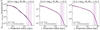 |
Fig. 4. Mean X-ray surface brightness profiles in the stellar mass bins: M★ = 1010.5−11 M⊙, corresponding to MW-like galaxies (left), M★ = 1011−11.25 M⊙ (centre), and M★ = 1011.25−11.5 M⊙ (right). The vertical dashed line is the mean R500c at 242.75 kpc (left), 369.01 kpc (centre), and 484.52 kpc (right) of the respective galaxy stellar mass bin with the shaded area corresponding to the minimum and maximum values. The black line is the analytical model, shown in Eq. (7), fit to the LC-TNG300 mean X-ray surface brightness profiles. The best-fitting parameters for the model are given in Table 3. We find decreasing values for the slope, β, with increasing stellar mass bins. |
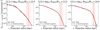 |
Fig. 5. Mean X-ray surface brightness profiles in the halo mass bins: M200m = 1012.5−13 M⊙, corresponding to MW-like galaxies (left), M200m = 1013−13.5 M⊙ (centre), and M200m = 1013.5−14 M⊙ (right). The vertical dashed line is the mean R500c at 246.35 kpc (left), 353.35 kpc (centre), and 519.34 kpc (right) of the respective halo mass bin with the shaded area corresponding to the minimum and maximum values. The black line is the analytical model, shown in Eq. (7), that fits the LC-TNG300 mean X-ray surface brightness profiles. The best-fitting parameters for the model are given in Table 4. We find decreasing values for the slope, β, with increasing halo mass bins. |
The model has two break radii, the core radius rc and the scale radius rs, where rc≪rs. The scale radius rs affects the profile at radii beyond R500c, the mean R500c of the stacked mass bin. The model also introduces two slope parameters, β, which influences the X-ray surface brightness profile at radii r<rs and ϵ, the slope that affects the profile at r>rs. As R500c is the radius used most commonly in observations, and β quantifies the shape of the profile at radii ≤R500c, we discuss here the variations in β across the stellar and halo mass bins.
The increasing stellar mass bins 1010.5−11 M⊙, 1011.25−11.5 M⊙, and 1011.25−11.5 M⊙ result in decreasing values of β from 0.4, 0.28, and 0.25, respectively. The same trend holds from the halo mass bins, where increasing halo mass bins 1012.5−13 M⊙, 1013−13.5 M⊙, and 1013.5−14 M⊙ have decreasing values of β from 0.57, 0.30, to 0.24, respectively. One of the reasons for the decrease is attributed to the mass-dependence of the feedback prescriptions in the TNG300 model, i.e., stellar mode dominating at lower masses, and the kinetic and thermal modes of energy injection by AGN dominating galaxies with M★≥1010.5 M⊙ (Weinberger et al. 2016). As discussed in Weinberger et al. (2018), the two AGN-related feedback channels depend on the black-hole (BH) accretion rates. For the high accretion rates, the thermal mode causes the gas cells close to the galactic centre to heat, eventually releasing the energy radiatively in X-rays. However, for lower accretion rates, the kinetic mode kicks in, depositing energy through winds and jets in random directions away from the BH. This causes gas heating and, hence, X-ray emission via cooling at a larger distance away from the galaxy centre, overall causing a flattening of the radial X-ray surface brightness profile as shown by the slope β in Figs. 4 and 5. This reasoning is further consolidated with studies detailing the effects of the kinetic mode of BH feedback in the TNG model (Terrazas et al. 2020), its impact on the gas properties, i.e., temperature, entropy, density, and CGM fraction (Zinger et al. 2020; Davies et al. 2020), and its correlation with X-ray emission (Truong et al. 2020, 2021; Oppenheimer et al. 2020; Ayromlou et al. 2023). Sorini et al. (2024) show a similar trend of decreasing slope for the gas density profiles with the SIMBA (Davé et al. 2019) suite of simulations. With simulation comparison projects like camels simulations (Villaescusa-Navarro et al. 2021), it is possible to study the correlation between X-ray emission around galaxies with different feedback implementations, the exploration of which we leave for a future study.
In the following two sections, we focus on how the projection effects result in deviations from the intrinsic profile. We discuss the effects on the stellar mass bins as it is an observationally available mass proxy.
5.2. Locally correlated environment
For the MW-mass bin, M★ = 1010.5−11 M⊙, with mean R200m = 525 kpc, we generate cubes within ±3 Mpc, ±9 Mpc and ±27 Mpc from the galaxy center. This corresponds to photons selected within ∼5.7×R200m, ∼17×R200m, and ∼51.4×R200m, respectively. Figure 6 presents the impact of the locally correlated LSS for MW-like halos. We show the intrinsic profile that is obtained by selecting events within ±R200m of the galaxy centre in purple. We compare our result with previous work from Oppenheimer et al. (2020), shown with the crosses in Fig. 6. They predict the profile between 10−242 kpc for a stellar mass sample in the mass range 108.2−11.39 M⊙ containing ∼400 galaxies. Their stellar mass sample is divided into low sSFR and high sSFR. We take the mean of the low sSFR and high sSFR profiles generated in their work and compare them with ours. The halo mass range corresponding to their stellar mass bin is 10∼12.3−13 M⊙, which entails the mean halo mass M200m = 1012.7 M⊙, same as that of the MW mass bin used in our work. Oppenheimer et al. (2020) use the TNG-100 simulation and synthesize mock X-ray observations for individual halos as opposed to this work that uses TNG300 and synthesizes mock X-ray observations within the lightcone. Despite these differences, this work's predicted X-ray intrinsic emission profiles are in good agreement with Oppenheimer et al. (2020).
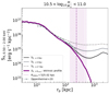 |
Fig. 6. Mean X-ray surface brightness profiles in the stellar mass bin M★=[1010.5, 1011] M⊙, corresponding to MW-like galaxies. The locally correlated large-scale structure contributions are shown by comparing the profiles obtained with photons selected within ±R200m (purple) and those obtained within ±3 Mpc (solid black), ±9 Mpc (solid grey), ±27 Mpc (dashed grey) away from the halo centre. The crosses are from previous work by Oppenheimer et al. (2020), where they generate mock X-ray observations using TNG-100. The vertical dashed line at 242 kpc and the dotted line at 525 kpc is the mean R500c and R200m, respectively, of the 5109 galaxies used in the mass bin with the shaded area corresponding to the minimum and maximum R500c values. The shaded uncertainties on the profiles represent the variance obtained by bootstrapping. |
We find that increasing the volume by  , i.e., by including events in ±3 Mpc, boosts the X-ray surface brightness profile at R200m by a factor of 5.2. We show this with the thick black line in Fig. 6. We find deviations from the true intrinsic profile due to events selected within ±3 Mpc at ∼150 kpc, which corresponds to ≈0.6×R500c and ≈0.3×R200m for the MW-stellar mass bin.
When considering the events in ±9 Mpc, i.e., increasing the volume used to compute the X-ray surface brightness profiles by  , we find that the X-ray surface brightness profile at R200m is boosted by a factor of 16.8 This is shown by the grey curve in Fig. 6. We find deviations from the true intrinsic profile due to events selected within ±9 Mpc, at ∼100 kpc, which corresponds to ≈0.4×R500c and ≈0.2×R200m for the MW-stellar mass bin.
For events selected in ±27 Mpc or by including events in a volume of  , the X-ray surface brightness profile at R200m is boosted by 47.3. This is shown by the light grey dashed curve in Fig. 6. The profile, in this case, remains unchanged only at radii ≤40 kpc, which corresponds to ≈0.2×R500c and ≈0.08×R200m for the MW-stellar mass bin.
In conclusion, we show for the first time the effect of the local environment on the true intrinsic profile of a mean MW-like stacked X-ray surface brightness profile. Namely, we find deviations from the true profile at ≈0.3×R200m, ≈0.2×R200m, and ≈0.08×R200m by including events out to ∼5.7×R200m, ∼17×R200m, and ∼51.4×R200m, respectively. The black, grey, and dashed-grey curves in Fig. 6 show that increasing the integration volume swamps the features of the intrinsic profile at radii closer to the galaxy centre.
In observations, one is sensitive to the complete line of sight towards the observer. Therefore, this effect can be corrected by subtracting a background emission level determined empirically from the observed surface brightness at a large distance from the halos of interest (assuming spherical symmetry in the large-scale emission). We test the impact of a simple, conventional background subtraction, where we subtract the mean value of the surface brightness profile beyond the R200m (vertical purple dotted line) from the respective grey, and dashed-grey curves in Fig. 6, as is most commonly done in observations. We find that the resulting profiles after background subtraction agree well with the intrinsic profile (solid purple line) out to R500c (the vertical dashed-dotted line). Beyond R500c, such a subtraction underestimates the X-ray emission at the outskirts. However, this must be further tested with larger-volume lightcones than used here (see further discussion in Sect. 6.1). Nevertheless, given the setup used in this work, we can, for the first time, probe this effect locally around the halo and show its impact in stacking experiments.
5.3. The effect of misclassified centrals
In simulations, we completely and accurately classify central and satellite galaxies within a given stellar mass bin. Using this to our advantage, here, we make a precise prediction of the average emission arising from stacking around satellite galaxies by considering the following fraction of satellite (or misclassified centrals) contaminating the total galaxy sample 0.01, 0.1 and 0.3. We select these contamination fractions of satellites by bootstrapping over the entire satellite galaxy sample. Table 1 details the number of centrals and satellites in the three stellar mass bins presented here. We show our findings in Figs. 7, 8, and 9, corresponding to stellar mass bins 1010.5−11 M⊙, 1011−11.25 M⊙, and 1011.25−11.5 M⊙, respectively.
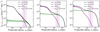 |
Fig. 7. Effect of centrals (purple) and misclassified-centrals (green), in the stellar mass bin M★=[1010.5, 1011] M⊙, on the total X-ray surface brightness profiles (black). The total sample is constructed such that there are 1% satellites and 99% centrals (left panel), 10% satellites and 90% centrals (middle panel), and 30% satellites and 70% centrals (right panel). The vertical dashed line at 242 kpc is the mean R500c of the 5109 galaxies used in the mass bin with the shaded area corresponding to the minimum and maximum values. The shaded regions on the profiles are the uncertainties obtained by bootstrapping. |
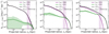 |
Fig. 8. Effect of centrals (purple) and misclassified-centrals (green), in the stellar mass bin M★=[1011, 1011.25] M⊙, on the total X-ray surface brightness profiles (black). The total sample is constructed with 1% (left panel), 10% (middle panel), and 30% (right panel) satellites. The vertical dashed line at 369 kpc is the mean R500c of the 680 galaxies used in the mass bin with the shaded area corresponding to the minimum and maximum values. |
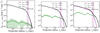 |
Fig. 9. Effect of centrals (purple) and misclassified-centrals (green), in the stellar mass bin M★=[1011.25, 1011.5] M⊙, on the total X-ray surface brightness profiles (black). The total sample is constructed with 1% (left panel), 10% (middle panel), and 30% (right panel) satellites. The vertical dashed line at 484.5 kpc is the mean R500c of the 305 galaxies used in the mass bin with the shaded area corresponding to the minimum and maximum values. |
Figure 7 quantifies the effect of misclassified centrals on the total surface brightness profile, shown with the solid black line, in the MW-stellar mass bin of 1010.5−11 M⊙. We show the integrated profile obtained by stacking only the satellite galaxies misclassified as centrals in green and the intrinsic profile due to central galaxies in purple. The point at which the profile due to misclassified centrals (green) intersects the intrinsic central galaxy (purple) profile represents the point at which the effect due to misclassified centrals contributes ∼50% to the total (centrals and satellites) emission. For a sample with 1% (left panel) and 10% (central panel) contaminating satellites, the effect due to misclassified centrals dominates over the intrinsic central galaxy emission at radii ≥1.04×R500c (∼252 kpc) and ≥0.24×R500c (∼59 kpc), respectively. In a sample with 30% satellites contaminants (right panel), the effect due to misclassified centrals dominates over the intrinsic central galaxy emission at radii ≥0.11×R500c (∼27 kpc).
Analogously, Fig. 8 quantifies the effect of misclassified centrals on the total surface brightness profile, shown with the solid black line, for galaxies in the stellar mass bin 1011−11.25 M⊙. For a sample with 1% (left panel) contaminating satellites, we find that the effect of misclassified centrals has negligible impact within radii ≤R500c. For 10% satellite contamination (central panel), the effect due to misclassified centrals dominates over the intrinsic central galaxy emission at radii ≥1.1×R500c (∼400 kpc) and for 30% satellites contamination (right panel), the effect due to misclassified centrals dominates over the intrinsic central galaxy emission at radii ≥0.63×R500c (∼231 kpc).
Finally, Fig. 9 quantifies this effect for the largest mass bin we are considering, 1011.25−11.5 M⊙. For a sample with 1% (left panel), 10% (centre panel) and 30% satellite contamination (right panel), the effect due to misclassified centrals remains negligible at all radii ≤R500c. More precisely, the 1% satellite contamination has a negligible impact on the total surface brightness profile. The 10% and 30% satellite contamination dominate over the intrinsic central galaxy profile at ≥1.7×R500c (∼804 kpc) and ≥1.2×R500c (∼565 kpc), respectively.
As expected, we find from Figs. 7, 8, and 9 that the effect due to misclassified centrals becomes increasingly important as we probe lower stellar mass bins in stacking experiments. As we go to higher mass bins, the decreasing impact of the effect of misclassified centrals is attributed to the satellites – of the same stellar mass bin – residing in less massive parent halos (see further explanation in Sect. 6).
Figure 10 presents the radial fraction of the X-ray emission from the intrinsic CGM – for four different levels of misclassified centrals contamination – in three stellar mass bins 1010.5−11 M⊙, 1011−11.25 M⊙, and 1011.25−11.5 M⊙, respectively. We complement the conclusions from Figs. 7, 8, and 9 by showing that for MW-like galaxies, the effect of misclassified centrals at the lowest contamination fraction of 0.01 results in the intrinsic central galaxy emission contributing only ∼51% of the total emission at R500c. This further deteriorates with the increasing fraction of misclassified centrals in the galaxy sample, where fractions of 0.1, 0.3, or 0.5 result in the intrinsic emission contributing ∼9%, ∼3% and ∼1% of the total emission at R500c, respectively. This effect is less pronounced for the intermediate and most massive stellar mass bins of 1011−11.25 M⊙ and 1011.25−11.5 M⊙ compared to the MW-like stellar mass bin. In the case of the 1011−11.25 M⊙ mass bin, for a fraction of misclassified centrals of 0.01, 0.1, 0.3, or 0.5, the central intrinsic emission contributes ∼93%, ∼55%, ∼23% and ∼11% of the total emission at R500c, respectively. Analogously, for the stellar mass bin of 1011.25−11.5 M⊙, for a fraction of misclassified centrals of 0.01, 0.1, 0.3, or 0.5, the central intrinsic emission contributes ∼99%, ∼86%, ∼61% and ∼40% of the total emission at R500c, respectively. Therefore, we present a clear trend of the increasing importance of the effect of misclassified centrals, not only due to the increasing fraction of satellite contamination in the galaxy sample but also due to the decreasing stellar mass bins.
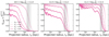 |
Fig. 10. Fraction of X-ray emission from the intrinsic hot CGM for different levels of satellite contamination (misclassified centrals) in the total galaxy sample. The fraction of X-ray emission from the intrinsic hot CGM for misclassified central contamination fractions of 0.01 (dotted line), 0.1 (dash-dotted line), 0.3 (dashed line), and 0.5 (solid line) are shown for three different mass bins: MW-like galaxies with stellar-masses in 1010.5−11 M⊙ (left panel), 1011−11.25 M⊙ (middle panel), and 1011.25−11.5 M⊙ (right panel). The shaded regions around each curve correspond to the uncertainty of the mean profile obtained by bootstrapping. The vertical black solid line at 242 kpc in the left panel, 369 kpc in the middle panel, and 484.5 kpc in the right panel corresponds to the mean R500c of the respective mass bins with the shaded area signifying the minimum and maximum values. We find that the contaminating effect of the misclassified centrals on the stacked profiles increases when the stellar mass decreases. |
6. Discussion
This work uses a TNG300-based forward model for the hot CGM emission and presents, for the first time, the effect of locally correlated large-scale structure around a halo, the effect of misclassified centrals in stacked hot CGM galactocentric profiles and the effect of the choice of centre. Our findings are vital in light of our explorations for studying X-ray emission around lower mass galaxies with stacking experiments. We divide the discussion of our results by focusing on the projection effects due to the locally correlated environment, first, in Sect. 6.1, second, the effect of misclassified centrals in Sect. 6.2, and lastly, the effect of miscentering in Sect. 6.3.
6.1. Locally correlated environment
The locally correlated environment for MW-like stellar mass galaxies boosts the mean galactocentric X-ray emission at radii ≤R200m. More precisely, at R200m the X-ray emission is boosted 5.2×, 16.8× and 47.3× by including emission ±3 Mpc, ±9 Mpc, ±27 Mpc away from the halo centre, respectively.
Increasing the volume over which the intrinsic galactocentric profiles are measured leads to increased X-ray emission at smaller radii. This increased X-ray emission, in projection, is attributed to the local environment in which the galaxy resides. The upturn in the black line in Fig. 6, corresponding to including events within ±3 Mpc (∼5.7R200m) of the galaxy centre, signifies the presence of other X-ray emitting halos ≳1 Mpc away from MW-like galaxies, i.e., ≈2×R200m or ≈4×R500c. This “upturn” feature is washed out as we start including events in even larger volumes, as shown by grey and dashed-grey lines (corresponding to events selected within ±9 Mpc and ±27 Mpc, respectively) in Fig. 6. This supports our finding that an observer starts probing the averaged hot gas emission from all galaxies in projection along the line of sight, drowning out the features due to the local environment when integrating events over larger volumes around a galaxy centre.
Further improvements to study this effect would involve including events to even larger radii around the galaxy. Given the limited area of the lightcone, 47.28 deg2, we are constrained in studying this effect out to ±27 Mpc. To quantify the effects of the locally correlated large-scale environment to even larger distances than those explored here, we need larger-volume lightcones, which is possible with larger cosmological hydrodynamical simulations like Magneticum (Dolag 2015), MillenniumTNG (Pakmor et al. 2023; Hernández-Aguayo et al. 2023), and FLAMINGO (Schaye et al. 2023). Additionally, future studies could study how different simulation feedback prescriptions can impact the trend observed in the X-ray surface brightness profiles by including events in larger volumes. It is particularly interesting to understand how the physics implemented in hydrodynamical simulations impacts the baryon spread around galaxies, i.e., the radius at which all the emissions converge to the mean background level in X-rays. We leave the study of these aspects to future work, which is made possible with the advent of projects like the camels simulations (Villaescusa-Navarro et al. 2021); see, e.g., Gebhardt et al. (2024) and Sorini et al. (2022).
6.2. The effect of misclassified centrals
We quantify the impact of the misclassified centrals (satellite-boost) residing in the same stellar mass bin as the central galaxies in Figs. 7, 8, and 9 for the stellar mass bins 1010.5−11, 1011−11.25, and 1011.25−11.5, respectively. For satellite galaxies with stellar masses of MW-like galaxies, the emission around satellites dominates over central emission because the satellites of the stellar mass range 1010.5−11 M⊙ reside in distinct halos with masses M200m = 1012.3−15.1, corresponding to a mean halo mass M200m = 1013.7 M⊙. We find that the satellite subhalos probe the emission of their parent halos, contributing to the stack with off-centred surface brightness profiles of their more massive parent halo. This contribution causes shallower slopes for the total emission (central and satellites) in the MW-stellar mass bin. In cases where 30%, 10%, or 1% of the satellites contribute to the total emission, we have shown that they dominate the measured total profile at radii ≥0.11×R500c, ≥0.24×R500c, and ≥1.04×R500c, respectively. We further investigate the effect of misclassified centrals in the more massive stellar mass bins of 1011−11.25 M⊙, and 1011.25−11.5 M⊙ in Figs. 8 and 9, respectively. We find the effect of misclassified centrals, with contamination fractions of 0.01, 0.1, and 0.3, less affects the 1011−11.25 M⊙, and 1011.25−11.5 M⊙ mass bins as opposed to the MW-stellar mass bin. We reaffirm this with the trend shown in Fig. 10, where the fraction of intrinsic emission at the mean R500c is lowest for the MW stellar mass bin for all contamination levels, as opposed to the more massive stellar mass bins.
To understand why the MW-stellar mass bin is most affected by the effect of misclassified centrals, we first look at the host halo masses of the satellites in the higher stellar mass bins of 1011−11.25 M⊙ and 1011.25−11.5 M⊙. These satellites reside in distinct halos of mean M200m ∼1014 M⊙ and ∼1014.2 M⊙, respectively. This is a direct implication arising from the difference in the stellar-to-halo-mass relation for central and satellite galaxies (Shuntov et al. 2022). Given that the mean halo mass of the central galaxies in the LC-TNG300 stellar mass bins of 1011−11.25 M⊙, and 1011.25−11.5 M⊙ is 1013.3 M⊙ and 1013.6 M⊙, respectively, we require large fraction of contamination to see the effect of misclassified centrals compared to that for the MW-stellar mass bin. More precisely, we find that the effect of misclassified centrals dominates over the central galaxy emission at R500c with satellite contamination fractions, fcont, sat, of 0.01, 0.14, and 0.77 for the stellar mass bins 1010.5−11 M⊙, 1011−11.25 M⊙, and 1011.25−11.5 M⊙, respectively. Hence, the contamination fractions probed here (fcont, sat = 0.01, 0.1, and 0.3), which are closer to the realistic fcont, sat in observations, do not significantly affect the stellar mass bins 1011−11.25, and 1011.25−11.5, respectively.
We now discuss how to observationally mitigate the effect of satellites misclassified as centrals using X-ray information. We investigate this issue here under the assumption that the observational galaxy sample is accurately classified into centrals and satellites; in such a case, the effect of misclassified centrals is dominated by instrument resolution, i.e., only satellite objects that are farther from the central than the distance corresponding to the instrument resolution can be easily disregarded as misidentified centrals. However, we must also note that using the X-ray information to mitigate the effect of satellites (based on their proximity to a central) requires the individual halos to be detected in X-rays, which, given the faintness of the CGM emission, is currently not viable for MW-mass halos with survey instruments like eROSITA (see further discussion in Sect. 6.3). For more massive (M31-like) halos, which have higher chances of detection in X-rays, we study how such segregation of misclassified centrals based on their proximity to a central in the sky would impact the mean X-ray surface brightness profile from misclassified centrals. We find that the mean X-ray profile from M31-mass satellite galaxies within 15″ of a central galaxy drops by 25% at R500c as opposed to the case where we consider all the satellite galaxies as misclassified centrals, as shown in Fig. 11. Therefore, such a technique for mitigating satellite contamination reduces the flattening of the mean X-ray surface brightness profile from satellites. However, an important caveat when selecting centrals without satellites in the vicinity is that such an experiment would give a biased result in the detected CGM itself, where one would be probing the CGM of galaxies only in isolated environments.
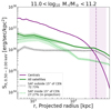 |
Fig. 11. Effect of further selection on the satellites misclassified as central galaxies on the X-ray surface brightness profile. The total population of satellites misclassified as centrals (solid green line) is divided into satellites within 15″ of a central (green dotted line) and satellites farther than 15″ from a central (grey dotted line) in projection on the sky. We show that satellites (misclassified as centrals) within 15″ of a central galaxy have a steeper profile than the case where we consider all the satellites, thereby reducing the overall flattening of the X-ray surface brightness profile due to misclassified centrals. Contrarily, the satellites farther than 15″ from a central have a constant surface brightness profile. The central galaxy profile is shown in purple. The vertical dashed line at 369 kpc is the mean R500c of the 680 galaxies used in the M31 stellar mass bin, and the shaded area corresponds to the minimum and maximum R500c value of the central galaxies in the M31-mass bin. The shaded uncertainties on the profiles represent the variance obtained by bootstrapping. |
Given these findings, we conclude that the contribution of satellites in MW-like galaxy samples containing satellites must not be neglected in stacking analysis. Observationally, to disentangle the contamination of the misclassified centrals, we must fit the profiles contributing to the intrinsic central galaxy jointly with the component capturing the effect of misclassified centrals for a given fraction of satellite contamination.
6.3. The effect of miscentering: X-ray centre offset from the centre defined by the minimum of the dark matter potential
Here, we study the effect of offset between the observationally defined X-ray centre and the centre defined by the minimum of the halo dark matter potential. The X-ray centre is computed using a luminosity-weighted average of all the counts within the spherical R200m cubes of the central halo. In this work, we use the input centre or the true centre as the location of the most bound particle within the halo as given by the FoF/Subfind algorithm applied on TNG300 to obtain halo catalogues. We use the projected positions on the sky for computing the offset, ΔX−ray−input, and convert these offsets to physical scales using the redshift of the halo. The mean of the ΔX−ray−input distribution is 70 kpc, with the 16th−84th percentiles ranging between 13−131 kpc, which is consistent with other works in literature (Seppi et al. 2023; Popesso et al. 2024). The corresponding mean value of the M200m distribution is at 1013.3 M⊙, i.e., within the M31-mass bin, with 16th−84th percentiles ranging between 1012.4−13.5 M⊙. The mean offset in the three halo mass bins considered in this work, 1012.5−13 M⊙, 1013−13.5 M⊙, and 1013.5−14 M⊙, are 52 kpc, 66 kpc, and 79 kpc, respectively; thereby, showing a correlation of increasing X-ray to true centre offset with increasing halo masses.
A galaxy stacking experiment with an eROSITA-like instrument that uses the dark matter halo potential minima as the centre would be affected by this miscentering effect. Assuming that the X-ray halo is detected, the objects for which the miscentering effect can be corrected are those where the offset between the X-ray and true centre is ≳30″, the resolution of eROSITA. In our lightcone, we report that ∼13% of objects have resolvable offsets (i.e., the offset separation ≳30″), which, if classified in M200m halo mass bins are as follows. For the 1012.5−13 M⊙ and 1013−13.5 M⊙ mass bins, 13% of objects have resolvable offsets; however, for the more massive 1013.5−14 M⊙ mass bin, 17% of objects have resolvable offsets. However, we must note that individual MW mass halos in X-rays with eROSITA are below the detection threshold. Therefore, detecting their X-ray peak is currently unfeasible, but might be possible with future observatories.
7. Summary
The main conclusions from this work are summarised as follows.
-
We present an analytical model (Eq. (7)) that well-describes the intrinsic SX-profile in LC-TNG300 across the stellar mass bins 1010.5−11 M⊙, 1011−11.25 M⊙, and 1011.25−11.5 M⊙ and halo mass bins of 1012.5−13 M⊙, 1013−13.5 M⊙, and 1013.5−14 M⊙. We provide the best-fitting parameters for the analytical model in Tables 3 and 4 for the stellar and halo mass bins explored in this work.
-
We carry forward the current state-of-the-art modelling analysis presented in Oppenheimer et al. (2020) by also showing the impact of the locally correlated environment on the measured X-ray surface brightness profiles.
-
We present, for the first time, the effect of misclassified centrals in stacking experiments for three stellar mass bins 1010.5−11 M⊙, 1011−11.25 M⊙, and 1011.25−11.5 M⊙. We find that the contaminating effect of the misclassified centrals on the stacked profiles increases when the stellar mass decreases.
-
For the MW-like galaxies, we conclude that the contribution of satellites (or misclassified centrals) can not be neglected in stacking analysis (see Fig. 10). In cases where 30%, 10%, or 1% of the satellites contribute to the total emission of MW-like galaxies, we have shown that they dominate the measured total SX profile at radii ≥0.11×R500c, ≥0.24×R500c, and ≥1.04×R500c, respectively.
-
We report the mean offset between the centre of the halo defined using the X-ray peak, and that obtained from the minimum of the halo potential is 70 kpc.
Modelling observed CGM profiles and comparing them with simulations is crucial to constrain the different galaxy formation models and to understand how the feedback and physics prescriptions affect the hot CGM profile. Current state-of-the-art cosmological hydrodynamical simulations are calibrated on the stellar mass function and successfully reproduce realistic galaxy populations. Despite this, Davies et al. (2020) show that EAGLE and IllustrisTNG predict different total gas mass fractions, affecting the observed CGM properties at MW-masses. Similarly, Khrykin et al. (2024) shows how the hot gas is sensitive to the different feedback variants within SIMBA. The model and methodology presented here provide the machinery to compare the measured hot CGM profiles among current simulations in future works.
Future X-ray missions, on the observation side, like Athena (Nandra et al. 2013), AXIS (Mushotzky et al. 2019), HUBS (Cui et al. 2020) will push our current detection limits and provide us with (i) the spatial resolution to reach higher redshifts, (ii) better quantify point-like source contamination within the hot CGM, (iii) the spectral resolution to allow disentangling components via spectral fitting and (iv) the grasp to reach even fainter surface brightness levels. This work, focusing on modelling the projection effects, is a step towards exploiting the information provided by the next-generation telescopes to better understand the intrinsic hot CGM emission. The prospects of this framework would be to extend it to interpret hot X-ray CGM measurements in stacking experiments by accounting for all projection effects, i.e., not only the impact due to the local environment of the halo and the effect due to misclassified centrals but also the emission from other X-ray sources such as AGN and XRB.
Data availability
The lightcone generation code, LightGen, is publicly available on GitLab8. The data underlying this article is available upon reasonable request to the corresponding author.
Acknowledgments
SS would like to thank Fulvio Ferlito, Matteo Guardiani, Christian Garrel, Emre Bahar, Jeremy Sanders, and the anonymous referee for all the useful scientific discussions. G.P. acknowledges financial support from the European Research Council (ERC) under the European Union's Horizon 2020 research and innovation program “Hot Milk” (grant agreement No. 865637) and support from Bando per il Finanziamento della Ricerca Fondamentale 2022 dell’Istituto Nazionale di Astrofisica (INAF): GO Large program and from the Framework per l’Attrazione e il Rafforzamento delle Eccellenze (FARE) per la ricerca in Italia (R20L5S39T9). Computations were performed on the HPC system Raven at the Max Planck Computing and Data Facility. We acknowledge the project support by the Max Planck Computing and Data Facility.
R500c is the radius at which the density of the halo is 500× the critical density of the universe.
R200m is the radius at which the density of the halo is 200× the mean matter density (cold dark matter and baryons).
See FAQ here: https://www.tng-project.org/data/docs/faq/
We define the surface brightness profiles in this work in units of erg/s/kpc2, consistent with Z+24, also called the luminosity profile.
References
- Ade, P. A., Aghanim, N., Arnaud, M., et al. 2016, A&A, 594, A13 [NASA ADS] [CrossRef] [EDP Sciences] [Google Scholar]
- Anders, E., & Grevesse, N. 1989, Geochim. Cosmochim., 53, 197 [NASA ADS] [CrossRef] [Google Scholar]
- Anderson, M. E., Gaspari, M., White, S. D., Wang, W., & Dai, X. 2015, MNRAS, 449, 3806 [NASA ADS] [CrossRef] [Google Scholar]
- Anderson, M. E., Churazov, E., & Bregman, J. N. 2016, MNRAS, 455, 227 [NASA ADS] [CrossRef] [Google Scholar]
- Ayromlou, M., Nelson, D., & Pillepich, A. 2023, MNRAS, 524, 5391 [CrossRef] [Google Scholar]
- Benson, A. J., Bower, R. G., Frenk, C. S., et al. 2003, ApJ, 599, 38 [NASA ADS] [CrossRef] [Google Scholar]
- Bertone, S., Schaye, J., Dalla Vecchia, C., et al. 2010, MNRAS, 407, 544 [NASA ADS] [CrossRef] [Google Scholar]
- Bhattacharyya, J., Das, S., Gupta, A., Mathur, S., & Krongold, Y. 2023, ApJ, 952, 41 [NASA ADS] [CrossRef] [Google Scholar]
- Biffi, V., Dolag, K., & Böhringer, H. 2013, MNRAS, 428, 1395 [Google Scholar]
- Biffi, V., Dolag, K., & Merloni, A. 2018, MNRAS, 481, 2213 [Google Scholar]
- Bogdán, Á., Forman, W. R., Kraft, R. P., & Jones, C. 2013a, ApJ, 772, 98 [CrossRef] [Google Scholar]
- Bogdán, Á., Forman, W. R., Vogelsberger, M., et al. 2013b, ApJ, 772, 97 [CrossRef] [Google Scholar]
- Bogdán, Á., Bourdin, H., Forman, W. R., et al. 2017, ApJ, 850, 98 [CrossRef] [Google Scholar]
- Bogdán, Á., Khabibullin, I., Kovács, O. E., et al. 2023, ApJ, 953, 42 [CrossRef] [Google Scholar]
- Bregman, J. N., Anderson, M. E., Miller, M. J., et al. 2018, ApJ, 862, 3 [NASA ADS] [CrossRef] [Google Scholar]
- Cappelluti, N., Arendt, R., Kashlinsky, A., et al. 2017, ApJ, 847, L11 [Google Scholar]
- Carlson, J., & White, M. 2010, ApJS, 190, 311 [NASA ADS] [CrossRef] [Google Scholar]
- Cavaliere, A., & Fusco-Femiano, R. 1976, A&A, 49, 137 [NASA ADS] [Google Scholar]
- Chadayammuri, U., Bogdán, Á., Oppenheimer, B. D., et al. 2022, ApJ, 936, L15 [NASA ADS] [CrossRef] [Google Scholar]
- Choudhury, P. P., Sharma, P., & Quataert, E. 2019, MNRAS, 488, 3195 [NASA ADS] [CrossRef] [Google Scholar]
- Comparat, J., Truong, N., Merloni, A., et al. 2022, A&A, 666, A156 [NASA ADS] [CrossRef] [EDP Sciences] [Google Scholar]
- Cooray, A., & Sheth, R. 2002, Phys. Rep., 372, 1 [Google Scholar]
- Cui, W., Power, C., Biffi, V., et al. 2016, MNRAS, 456, 2566 [NASA ADS] [CrossRef] [Google Scholar]
- Cui, W., Chen, L. -B., Gao, B., et al. 2020, J. Low Temp. Phys., 199, 502 [NASA ADS] [CrossRef] [Google Scholar]
- Das, S., Mathur, S., Gupta, A., et al. 2019, ApJ, 885, 108 [NASA ADS] [CrossRef] [Google Scholar]
- Das, S., Chiang, Y. K., & Mathur, S. 2023, ApJ, 951, 125 [NASA ADS] [CrossRef] [Google Scholar]
- Davé, R., Anglés-Alcázar, D., Narayanan, D., et al. 2019, MNRAS, 486, 2827 [Google Scholar]
- Davies, J. J., Crain, R. A., Oppenheimer, B. D., & Schaye, J. 2020, MNRAS, 491, 4462 [NASA ADS] [CrossRef] [Google Scholar]
- De Luca, A., & Molendi, S. 2004, A&A, 419, 837 [NASA ADS] [CrossRef] [EDP Sciences] [Google Scholar]
- Dekel, A., & Silk, J. 1986, ApJ, 303, 39 [Google Scholar]
- Dekel, A., & Woo, J. 2003, MNRAS, 344, 1131 [NASA ADS] [CrossRef] [Google Scholar]
- Diemer, B., Mansfield, P., Kravtsov, A. V., & More, S. 2017, ApJ, 843, 140 [NASA ADS] [CrossRef] [Google Scholar]
- Dolag, K. 2015, IAU General Assembly, 29, 2250156 [Google Scholar]
- Dolag, K., Borgani, S., Murante, G., & Springel, V. 2009, MNRAS, 399, 497 [Google Scholar]
- Eckert, D., Gaspari, M., Gastaldello, F., Le Brun, A. M., & O’Sullivan, E. 2021, Universe, 7, 142 [NASA ADS] [CrossRef] [Google Scholar]
- Fabian, A. C. 2012, ARA&A, 50, 455 [Google Scholar]
- Faerman, Y., & Werk, J. K. 2023, ApJ, 956, 92 [NASA ADS] [CrossRef] [Google Scholar]
- Faerman, Y., Sternberg, A., & McKee, C. F. 2017, ApJ, 835, 52 [NASA ADS] [CrossRef] [Google Scholar]
- Faucher-Giguère, C. -A., & Oh, S. P. 2023, ARA&A, 61, 131 [CrossRef] [Google Scholar]
- Foster, A., Ji, L., Smith, R., & Brickhouse, N. 2012, ApJ, 756, 128 [Google Scholar]
- Galeazzi, M., Gupta, A., Covey, K., & Ursino, E. 2007, ApJ, 658, 1081 [NASA ADS] [CrossRef] [Google Scholar]
- Gebhardt, M., Anglés-Alcázar, D., Borrow, J., et al. 2024, MNRAS, 529, 4896 [NASA ADS] [CrossRef] [Google Scholar]
- Gilli, R., Comastri, A., & Hasinger, G. 2007, A&A, 463, 79 [NASA ADS] [CrossRef] [EDP Sciences] [Google Scholar]
- Gupta, A., Mathur, S., Kingsbury, J., Das, S., & Krongold, Y. 2023, Nat. Astron., 7, 799 [NASA ADS] [CrossRef] [Google Scholar]
- Henley, D. B., & Shelton, R. L. 2010, ApJS, 187, 388 [NASA ADS] [CrossRef] [Google Scholar]
- Henley, D. B., & Shelton, R. L. 2012, ApJS, 202, 14 [NASA ADS] [CrossRef] [Google Scholar]
- Henley, D. B., & Shelton, R. L. 2013, ApJ, 773, 92 [NASA ADS] [CrossRef] [Google Scholar]
- Hernández-Aguayo, C., Springel, V., Pakmor, R., et al. 2023, MNRAS, 524, 2556 [CrossRef] [Google Scholar]
- Hikage, C., Mandelbaum, R., Leauthaud, A., Rozo, E., & Rykoff, E. S. 2018, MNRAS, 480, 2689 [CrossRef] [Google Scholar]
- Hoshino, H., Leauthaud, A., Lackner, C., et al. 2015, MNRAS, 452, 998 [NASA ADS] [CrossRef] [Google Scholar]
- Kaaret, P., Koutroumpa, D., Kuntz, K., et al. 2020, Nat. Astron., 4, 1072 [CrossRef] [Google Scholar]
- Khrykin, I. S., Sorini, D., Lee, K. -G., & Davé, R. 2024, MNRAS, 529, 537 [NASA ADS] [CrossRef] [Google Scholar]
- Koutroumpa, D., Acero, F., Lallement, R., Ballet, J., & Kharchenko, V. 2007, A&A, 475, 901 [NASA ADS] [CrossRef] [EDP Sciences] [Google Scholar]
- Kravtsov, A. V., Berlind, A. A., Wechsler, R. H., et al. 2004, ApJ, 609, 35 [Google Scholar]
- Lauer, T. R., Postman, M., Strauss, M. A., Graves, G. J., & Chisari, N. E. 2014, ApJ, 797, 82 [Google Scholar]
- Le Brun, A. M., McCarthy, I. G., Schaye, J., & Ponman, T. J. 2014, MNRAS, 441, 1270 [NASA ADS] [CrossRef] [Google Scholar]
- Li, J. -T., Bregman, J. N., Wang, Q. D., et al. 2017, ApJS, 233, 20 [NASA ADS] [CrossRef] [Google Scholar]
- Lim, S., Barnes, D., Vogelsberger, M., et al. 2021, MNRAS, 504, 5131 [CrossRef] [Google Scholar]
- Locatelli, N., Ponti, G., Zheng, X., et al. 2024, A&A, 681, A78 [NASA ADS] [CrossRef] [EDP Sciences] [Google Scholar]
- Luo, B., Brandt, W., Xue, Y., et al. 2016, ApJS, 228, 2 [CrossRef] [Google Scholar]
- Lyskova, N., Churazov, E., Khabibullin, I., et al. 2023, MNRAS, 525, 898 [NASA ADS] [CrossRef] [Google Scholar]
- Marinacci, F., Vogelsberger, M., Pakmor, R., et al. 2018, MNRAS, 480, 5113 [NASA ADS] [Google Scholar]
- Martel, H., Robichaud, F., & Barai, P. 2014, ApJ, 786, 79 [NASA ADS] [CrossRef] [Google Scholar]
- Mathur, S., Das, S., Gupta, A., & Krongold, Y. 2023, MNRAS, 525, L11 [Google Scholar]
- McKee, C. F., & Ostriker, J. P. 1977, ApJ, 218, 148 [NASA ADS] [CrossRef] [Google Scholar]
- Merson, A. I., Baugh, C. M., Helly, J. C., et al. 2013, MNRAS, 429, 556 [NASA ADS] [CrossRef] [Google Scholar]
- Miller, M. J., & Bregman, J. N. 2015, ApJ, 800, 14 [NASA ADS] [CrossRef] [Google Scholar]
- Mushotzky, R., Aird, J., Barger, A. J., et al. 2019, BAAS, 51, 107 [Google Scholar]
- Naiman, J. P., Pillepich, A., Springel, V., et al. 2018, MNRAS, 477, 1206 [Google Scholar]
- Nakashima, S., Inoue, Y., Yamasaki, N., et al. 2018, ApJ, 862, 34 [CrossRef] [Google Scholar]
- Nandra, K., Barret, D., Barcons, X., et al. 2013, arXiv e-prints [arXiv:arXiv:1306.2307] [Google Scholar]
- Nelson, D., Pillepich, A., Genel, S., et al. 2015, Astron. Comput., 13, 12 [Google Scholar]
- Nelson, D., Springel, V., Pillepich, A., et al. 2019, Comput. Astrophys. Cosmol., 6, 1 [NASA ADS] [CrossRef] [Google Scholar]
- Nelson, D., Byrohl, C., Ogorzalek, A., et al. 2023, MNRAS, 522, 3665 [NASA ADS] [CrossRef] [Google Scholar]
- Oguri, M., & Takada, M. 2011, Phys. Rev. D, 83, 023008 [NASA ADS] [CrossRef] [Google Scholar]
- Oguri, M., Lin, Y. -T., Lin, S. -C., et al. 2018, PASJ, 70, S20 [Google Scholar]
- Oppenheimer, B. D., Bogdán, Á., Crain, R. A., et al. 2020, ApJ, 893, L24 [NASA ADS] [CrossRef] [Google Scholar]
- Oren, Y., Sternberg, A., McKee, C. F., Faerman, Y., & Genel, S. 2024, ApJ, 974, 291 [Google Scholar]
- Ostriker, E. C., & Shetty, R. 2011, ApJ, 731, 41 [Google Scholar]
- Pakmor, R., Springel, V., Coles, J. P., et al. 2023, MNRAS, 524, 2539 [NASA ADS] [CrossRef] [Google Scholar]
- Pan, Z., Qu, Z., Bregman, J. N., & Liu, J. 2024, ApJS, 271, 62 [NASA ADS] [CrossRef] [Google Scholar]
- Pandya, V., Fielding, D. B., Bryan, G. L., et al. 2023, ApJ, 956, 118 [NASA ADS] [CrossRef] [Google Scholar]
- Pillepich, A., Nelson, D., Hernquist, L., et al. 2018a, MNRAS, 475, 648 [Google Scholar]
- Pillepich, A., Springel, V., Nelson, D., et al. 2018b, MNRAS, 473, 4077 [Google Scholar]
- Ponti, G., Zheng, X., Locatelli, N., et al. 2023, A&A, 674, A195 [NASA ADS] [CrossRef] [EDP Sciences] [Google Scholar]
- Popesso, P., Marini, I., Dolag, K., et al. 2024, A&A, submitted [Google Scholar]
- Rahmati, A., Schaye, J., Crain, R. A., et al. 2016, MNRAS, 459, 310 [NASA ADS] [CrossRef] [Google Scholar]
- Rohr, E., Pillepich, A., Nelson, D., Ayromlou, M., & Zinger, E. 2024, A&A, 686, A86 [NASA ADS] [CrossRef] [EDP Sciences] [Google Scholar]
- Saro, A., Bocquet, S., Rozo, E., et al. 2015, MNRAS, 454, 2305 [Google Scholar]
- Schaye, J., Kugel, R., Schaller, M., et al. 2023, MNRAS, 526, 4978 [NASA ADS] [CrossRef] [Google Scholar]
- Schellenberger, G., Bogdán, Á., ZuHone, J. A., et al. 2024, ApJ, 969, 85 [Google Scholar]
- Seppi, R., Comparat, J., Nandra, K., et al. 2023, A&A, 671, A57 [NASA ADS] [CrossRef] [EDP Sciences] [Google Scholar]
- Shuntov, M., McCracken, H., Gavazzi, R., et al. 2022, A&A, 664, A61 [NASA ADS] [CrossRef] [EDP Sciences] [Google Scholar]
- Silk, J., & Rees, M. J. 1998, A&A, 331, L1 [NASA ADS] [Google Scholar]
- Singh, P., Voit, G., & Nath, B. B. 2021, MNRAS, 501, 2467 [Google Scholar]
- Singh, P., Lau, E. T., Faerman, Y., Stern, J., & Nagai, D. 2024, MNRAS, 532, 3222 [NASA ADS] [CrossRef] [Google Scholar]
- Skibba, R. A., van den Bosch, F. C., Yang, X., et al. 2011, MNRAS, 410, 417 [NASA ADS] [CrossRef] [Google Scholar]
- Smith, R. K., Brickhouse, N. S., Liedahl, D. A., & Raymond, J. C. 2001, ApJ, 556, L91 [Google Scholar]
- Sorini, D., Davé, R., Cui, W., & Appleby, S. 2022, MNRAS, 516, 883 [CrossRef] [Google Scholar]
- Sorini, D., Bose, S., Davé, R., & Anglés-Alcázar, D. 2024, OJAp, 7, 115 [Google Scholar]
- Springel, V., & Hernquist, L. 2003, MNRAS, 339, 289 [Google Scholar]
- Springel, V., White, S. D., Tormen, G., & Kauffmann, G. 2001, MNRAS, 328, 726 [NASA ADS] [CrossRef] [Google Scholar]
- Springel, V., Pakmor, R., Pillepich, A., et al. 2018, MNRAS, 475, 676 [Google Scholar]
- Stern, J., Fielding, D., Hafen, Z., et al. 2024, MNRAS, 530, 1711 [NASA ADS] [CrossRef] [Google Scholar]
- Strickland, D. K., & Heckman, T. M. 2009, ApJ, 697, 2030 [Google Scholar]
- Sunyaev, R., & Zeldovich, Y. B. 1972, A&A, 20, 189 [Google Scholar]
- Terrazas, B. A., Bell, E. F., Pillepich, A., et al. 2020, MNRAS, 493, 1888 [Google Scholar]
- Truong, N., Pillepich, A., Werner, N., et al. 2020, MNRAS, 494, 549 [NASA ADS] [CrossRef] [Google Scholar]
- Truong, N., Pillepich, A., & Werner, N. 2021, MNRAS, 501, 2210 [NASA ADS] [CrossRef] [Google Scholar]
- Truong, N., Pillepich, A., Nelson, D., et al. 2023, MNRAS, 525, 1976 [NASA ADS] [CrossRef] [Google Scholar]
- Tumlinson, J., Peeples, M. S., & Werk, J. K. 2017, ARA&A, 55, 389 [Google Scholar]
- van de Voort, F. 2013, MNRAS, 430, 2688 [NASA ADS] [CrossRef] [Google Scholar]
- Vikhlinin, A., Kravtsov, A., Forman, W., et al. 2006, ApJ, 640, 691 [Google Scholar]
- Vikram, V., Lidz, A., & Jain, B. 2017, MNRAS, 467, 2315 [NASA ADS] [Google Scholar]
- Villaescusa-Navarro, F., Anglés-Alcázar, D., Genel, S., et al. 2021, ApJ, 915, 71 [NASA ADS] [CrossRef] [Google Scholar]
- Vladutescu-Zopp, S., Biffi, V., & Dolag, K. 2023, A&A, 669, A34 [NASA ADS] [CrossRef] [EDP Sciences] [Google Scholar]
- Vladutescu-Zopp, S., Biffi, V., & Dolag, K. 2025, A&A, 695, A2 [NASA ADS] [CrossRef] [EDP Sciences] [Google Scholar]
- Voit, G. M., Donahue, M., Zahedy, F., et al. 2019, ApJ, 879, L1 [Google Scholar]
- Wechsler, R. H., & Tinker, J. L. 2018, ARA&A, 56, 435 [NASA ADS] [CrossRef] [Google Scholar]
- Weinberger, R., Springel, V., Hernquist, L., et al. 2016, MNRAS, 465, 3291 [Google Scholar]
- Weinberger, R., Springel, V., Pakmor, R., et al. 2018, MNRAS, 479, 4056 [Google Scholar]
- Weng, S., Péroux, C., Ramesh, R., et al. 2024, MNRAS, 527, 3494 [Google Scholar]
- White, S. D., & Rees, M. J. 1978, MNRAS, 183, 341 [NASA ADS] [CrossRef] [Google Scholar]
- Wijers, N. A. 2022, MNRAS, 514, 5214 [NASA ADS] [CrossRef] [Google Scholar]
- Wijers, N. A., Schaye, J., Oppenheimer, B. D., Crain, R. A., & Nicastro, F. 2019, MNRAS, 488, 2947 [NASA ADS] [CrossRef] [Google Scholar]
- Wijers, N. A., Schaye, J., & Oppenheimer, B. D. 2020, MNRAS, 498, 574 [NASA ADS] [CrossRef] [Google Scholar]
- Yeung, M. C., Ponti, G., Freyberg, M. J., et al. 2024, A&A, 690, A399 [NASA ADS] [CrossRef] [EDP Sciences] [Google Scholar]
- Zhang, Y., Jeltema, T., Hollowood, D., et al. 2019, MNRAS, 487, 2578 [NASA ADS] [CrossRef] [Google Scholar]
- Zhang, Y., Comparat, J., Ponti, G., et al. 2024, A&A, 690, A267 [NASA ADS] [CrossRef] [EDP Sciences] [Google Scholar]
- Zheng, X., Locatelli, G. P. N., Sanders, J., et al. 2024, A&A, 689, A328 [NASA ADS] [CrossRef] [EDP Sciences] [Google Scholar]
- Zinger, E., Pillepich, A., Nelson, D., et al. 2020, MNRAS, 499, 768 [CrossRef] [Google Scholar]
- Zitrin, A., Bartelmann, M., Umetsu, K., Oguri, M., & Broadhurst, T. 2012, MNRAS, 426, 2944 [Google Scholar]
- ZuHone, J. A., & Hallman, E. J. 2016, Astrophysics Source Code Library [record ascl:1608.002] [Google Scholar]
- ZuHone, J. A., Schellenberger, G., Ogorzałek, A., et al. 2024, ApJ, 967, 49 [NASA ADS] [CrossRef] [Google Scholar]
All Tables
All Figures
|
Fig. 1. Illustration of the lightcone built using TNG300 in the x−y plane. The figure shows the subhalos within LC-TNG300 at 0.03≤z≤0.3 remapped using boxremap (Carlson & White 2010). The observer is set at the (0, 0, 0) location. The lightcone goes out to 1231 cMpc along the x-axis, subtending an area of 47.28 deg2 on the sky in the y−z plane. The subhalos are colour-coded with their stellar masses. |
| In the text | |
|
Fig. 2. Projected rest-frame X-ray events from the TNG300 ligthcone in the 0.5−2.0 keV band for a telescope with energy-independent collecting area 1000 cm2 and exposure time of 1000 ks. The events are generated using the hot gas cells within the TNG300 lightcone at redshifts 0.03−0.3 using pyXsim (ZuHone & Hallman 2016). The centre for the projection onto the sky is chosen as RA, Dec ≡ (0., 0.) degrees. The contours represent the two X-ray surface brightness levels of 5×10⁻¹⁴ erg s−1 cm−2 arcmin−2 and 2×10⁻¹⁶ erg s−1 cm−2 arcmin−2. |
| In the text | |
|
Fig. 3. Projected halos (centrals) are overplotted with their corresponding scaled R500c at z = 0.3; the R500c of the halos are represented by the size of the circles. We also show the projected rest-frame X-ray events from the TNG300 ligthcone in the 0.5−2.0 keV band for a telescope with energy-independent collecting area 1000 cm2 and exposure time of 1000 ks at the redshift slice of 0.284≤z≤0.3. The halos with M200m∈1014−14.5 M⊙ are shown in red, M200m∈1013.5−14 M⊙ in grey, M200m∈1013−13.5 M⊙ in cyan, and M200m∈1012.5−13 M⊙ in blue. |
| In the text | |
|
Fig. 4. Mean X-ray surface brightness profiles in the stellar mass bins: M★ = 1010.5−11 M⊙, corresponding to MW-like galaxies (left), M★ = 1011−11.25 M⊙ (centre), and M★ = 1011.25−11.5 M⊙ (right). The vertical dashed line is the mean R500c at 242.75 kpc (left), 369.01 kpc (centre), and 484.52 kpc (right) of the respective galaxy stellar mass bin with the shaded area corresponding to the minimum and maximum values. The black line is the analytical model, shown in Eq. (7), fit to the LC-TNG300 mean X-ray surface brightness profiles. The best-fitting parameters for the model are given in Table 3. We find decreasing values for the slope, β, with increasing stellar mass bins. |
| In the text | |
|
Fig. 5. Mean X-ray surface brightness profiles in the halo mass bins: M200m = 1012.5−13 M⊙, corresponding to MW-like galaxies (left), M200m = 1013−13.5 M⊙ (centre), and M200m = 1013.5−14 M⊙ (right). The vertical dashed line is the mean R500c at 246.35 kpc (left), 353.35 kpc (centre), and 519.34 kpc (right) of the respective halo mass bin with the shaded area corresponding to the minimum and maximum values. The black line is the analytical model, shown in Eq. (7), that fits the LC-TNG300 mean X-ray surface brightness profiles. The best-fitting parameters for the model are given in Table 4. We find decreasing values for the slope, β, with increasing halo mass bins. |
| In the text | |
|
Fig. 6. Mean X-ray surface brightness profiles in the stellar mass bin M★=[1010.5, 1011] M⊙, corresponding to MW-like galaxies. The locally correlated large-scale structure contributions are shown by comparing the profiles obtained with photons selected within ±R200m (purple) and those obtained within ±3 Mpc (solid black), ±9 Mpc (solid grey), ±27 Mpc (dashed grey) away from the halo centre. The crosses are from previous work by Oppenheimer et al. (2020), where they generate mock X-ray observations using TNG-100. The vertical dashed line at 242 kpc and the dotted line at 525 kpc is the mean R500c and R200m, respectively, of the 5109 galaxies used in the mass bin with the shaded area corresponding to the minimum and maximum R500c values. The shaded uncertainties on the profiles represent the variance obtained by bootstrapping. |
| In the text | |
|
Fig. 7. Effect of centrals (purple) and misclassified-centrals (green), in the stellar mass bin M★=[1010.5, 1011] M⊙, on the total X-ray surface brightness profiles (black). The total sample is constructed such that there are 1% satellites and 99% centrals (left panel), 10% satellites and 90% centrals (middle panel), and 30% satellites and 70% centrals (right panel). The vertical dashed line at 242 kpc is the mean R500c of the 5109 galaxies used in the mass bin with the shaded area corresponding to the minimum and maximum values. The shaded regions on the profiles are the uncertainties obtained by bootstrapping. |
| In the text | |
|
Fig. 8. Effect of centrals (purple) and misclassified-centrals (green), in the stellar mass bin M★=[1011, 1011.25] M⊙, on the total X-ray surface brightness profiles (black). The total sample is constructed with 1% (left panel), 10% (middle panel), and 30% (right panel) satellites. The vertical dashed line at 369 kpc is the mean R500c of the 680 galaxies used in the mass bin with the shaded area corresponding to the minimum and maximum values. |
| In the text | |
|
Fig. 9. Effect of centrals (purple) and misclassified-centrals (green), in the stellar mass bin M★=[1011.25, 1011.5] M⊙, on the total X-ray surface brightness profiles (black). The total sample is constructed with 1% (left panel), 10% (middle panel), and 30% (right panel) satellites. The vertical dashed line at 484.5 kpc is the mean R500c of the 305 galaxies used in the mass bin with the shaded area corresponding to the minimum and maximum values. |
| In the text | |
|
Fig. 10. Fraction of X-ray emission from the intrinsic hot CGM for different levels of satellite contamination (misclassified centrals) in the total galaxy sample. The fraction of X-ray emission from the intrinsic hot CGM for misclassified central contamination fractions of 0.01 (dotted line), 0.1 (dash-dotted line), 0.3 (dashed line), and 0.5 (solid line) are shown for three different mass bins: MW-like galaxies with stellar-masses in 1010.5−11 M⊙ (left panel), 1011−11.25 M⊙ (middle panel), and 1011.25−11.5 M⊙ (right panel). The shaded regions around each curve correspond to the uncertainty of the mean profile obtained by bootstrapping. The vertical black solid line at 242 kpc in the left panel, 369 kpc in the middle panel, and 484.5 kpc in the right panel corresponds to the mean R500c of the respective mass bins with the shaded area signifying the minimum and maximum values. We find that the contaminating effect of the misclassified centrals on the stacked profiles increases when the stellar mass decreases. |
| In the text | |
|
Fig. 11. Effect of further selection on the satellites misclassified as central galaxies on the X-ray surface brightness profile. The total population of satellites misclassified as centrals (solid green line) is divided into satellites within 15″ of a central (green dotted line) and satellites farther than 15″ from a central (grey dotted line) in projection on the sky. We show that satellites (misclassified as centrals) within 15″ of a central galaxy have a steeper profile than the case where we consider all the satellites, thereby reducing the overall flattening of the X-ray surface brightness profile due to misclassified centrals. Contrarily, the satellites farther than 15″ from a central have a constant surface brightness profile. The central galaxy profile is shown in purple. The vertical dashed line at 369 kpc is the mean R500c of the 680 galaxies used in the M31 stellar mass bin, and the shaded area corresponds to the minimum and maximum R500c value of the central galaxies in the M31-mass bin. The shaded uncertainties on the profiles represent the variance obtained by bootstrapping. |
| In the text | |
Current usage metrics show cumulative count of Article Views (full-text article views including HTML views, PDF and ePub downloads, according to the available data) and Abstracts Views on Vision4Press platform.
Data correspond to usage on the plateform after 2015. The current usage metrics is available 48-96 hours after online publication and is updated daily on week days.
Initial download of the metrics may take a while.