| Issue |
A&A
Volume 696, April 2025
|
|
|---|---|---|
| Article Number | A89 | |
| Number of page(s) | 19 | |
| Section | Extragalactic astronomy | |
| DOI | https://doi.org/10.1051/0004-6361/202453570 | |
| Published online | 08 April 2025 | |
Galaxy And Mass Assembly (GAMA): Environment-dependent galaxy stellar mass functions in the low-redshift Universe
1
Hamburger Sternwarte, Universität Hamburg, Gojenbergsweg 112, 21029 Hamburg, Germany
2
Cluster of Excellence Quantum Universe, Universität Hamburg, Luruper Chaussee 149, 22761 Hamburg, Germany
3
International Centre for Radio Astronomy Research (ICRAR), University of Western Australia, Crawley, WA 6009, Australia
4
Centre for Astrophysics and Supercomputing, Swinburne University of Technology, Hawthorn, VIC 3122, Australia
⋆ Corresponding author; This email address is being protected from spambots. You need JavaScript enabled to view it.
Received:
20
December
2024
Accepted:
13
February
2025
Abstract
From a carefully selected sample of 52 089 galaxies and 10 429 groups, we investigate the variation of the low-redshift galaxy stellar mass function (GSMF) in the equatorial Galaxy And Mass Assembly (GAMA) dataset as a function of four different environmental properties. We find that: (i) The GSMF is not strongly affected by distance to the nearest filament but rather by group membership. (ii) More massive halos tend to host more massive galaxies and exhibit a steeper decline with stellar mass in the number of intermediate-mass galaxies. This result is robust against the choice of dynamical and luminosity-based group halo mass estimates. (iii) The GSMF of group galaxies does not depend on the position within a filament, but for groups outside of filaments, the characteristic mass of the GSMF is lower. Finally, our global GSMF is well described by a double Schechter function with the following parameters: log[M⋆/(M⊙h70−2)] = 10.76 ± 0.01, Φ1⋆ = (3.75 ± 0.09)×10−3 Mpc−3 h703, α1 = −0.86 ± 0.03, Φ2⋆ = (0.13 ± 0.05)×10−3 Mpc−3 h703, and α2 = −1.71 ± 0.06. This result is consistent with previous GAMA studies in terms of M⋆, although we find lower values for both α1 and α2.
Key words: galaxies: distances and redshifts / galaxies: evolution / galaxies: fundamental parameters / galaxies: luminosity function / mass function / galaxies: stellar content / large-scale structure of Universe
© The Authors 2025
 Open Access article, published by EDP Sciences, under the terms of the Creative Commons Attribution License (https://creativecommons.org/licenses/by/4.0), which permits unrestricted use, distribution, and reproduction in any medium, provided the original work is properly cited.
This article is published in open access under the Subscribe to Open model. This email address is being protected from spambots. You need JavaScript enabled to view it. to support open access publication.
1. Introduction
According to the Λ cold dark matter (ΛCDM) cosmological paradigm, structures in the present Universe arose from hierarchical clustering, whereby smaller dark matter halos (DMHs) grew by gravitational attraction first and progressively merged into larger halos (Press & Schechter 1974; Blumenthal et al. 1984; Davis et al. 1985). Baryons gathered in the centres of these halos, and a small fraction of them cooled and subsequently condensed into stars to form galaxies (White & Rees 1978; White & Frenk 1991). However, DMHs – and hence the galaxies residing within them – are not isolated. They are part of a large-scale structure (LSS; Kaiser 1984; Efstathiou et al. 1988), also known as the ‘cosmic web’ (Jõeveer et al. 1978; Bond et al. 1996). Under the effect of gravity across cosmic time, the cosmic web emerged from the anisotropic collapse of the initial fluctuations of the matter density field (Zel’dovich 1970). This web consists of sizeable, nearly empty voids surrounded by sheet-like walls formed by filaments intersecting at the locations of clusters of galaxies. These nodes represent the densest regions of the LSS, containing a large fraction of the dark matter mass (Bond & Myers 1996; Pogosyan et al. 1996).
The galaxy stellar mass function (GSMF; Bell et al. 2003; Baldry et al. 2008, 2012; Wright et al. 2017; Driver et al. 2022), which gives the number density of galaxies per unit mass, is one of the most fundamental measurements in extragalactic astronomy, containing valuable information about the physical processes of galaxy formation and evolution. GSMFs were first measured in the optical and later in the near-infrared (NIR), where the light better traces the low-mass stellar populations that dominate the stellar mass reservoir. In fact, the stellar masses of galaxies may be derived from optical and/or NIR photometry (Larson & Tinsley 1978; Jablonka & Arimoto 1992; Bell & de Jong 2001), where, generally speaking, a broader wavelength coverage results in a higher precision, or from spectroscopy (Kauffmann et al. 2003; Panter et al. 2004; Gallazzi et al. 2005). Multi-wavelength photometric and spectroscopic surveys such as the Sloan Digital Sky Survey (SDSS) and the Galaxy And Mass Assembly (GAMA) survey are thus able to estimate stellar masses with a precision of ∼0.2 dex (Taylor et al. 2011), and the most significant measurements of the GSMF obtained from SDSS (Bell et al. 2003; Baldry et al. 2008) and GAMA (Baldry et al. 2012; Wright et al. 2017), in which the GSMF was probed to a stellar mass limit of 108 M⊙, are in reasonable agreement.
While the integral of the GSMF defines the density of baryonic mass currently bound in stars, and thus the global star formation (SF) efficiency, its shape (a power-law with an exponential cut-off at high masses) is related to the evolutionary processes governing SF. Explaining the shape of the GSMF (relative to that of the robustly predicted halo mass function) is one of the major aims of galaxy formation theory. The shape of the GSMF is generally thought to be related to two different feedback mechanisms that are responsible for suppressing SF. At low halo masses, supernova feedback creating galactic winds plays a crucial role in regulating SF (Larson 1974; Dekel & Silk 1986; Pillepich et al. 2018; Scharré et al. 2024), while Oppenheimer et al. (2010) claimed that the re-accretion of these winds is essential in shaping the GSMF. At higher masses, initially infalling gas is heated by a virial shock (Dekel & Birnboim 2006) and subsequently prevented from cooling by feedback from active galactic nuclei, thereby suppressing SF (Kereš et al. 2005; Croton et al. 2006; Pillepich et al. 2018; Scharré et al. 2024). Both of these feedback processes have a mass dependence; that is, the efficiency with which they suppress SF depends on halo mass. Additionally, mergers will also modify the GSMF by moving galaxies from lower to higher masses, which may even be the dominant process shaping the GSMF at masses greater than 1010.8 M⊙ (Robotham et al. 2014). The mass dependencies of all of these processes shape the GSMF, and since these are in turn expected to depend on the environment, the GSMF should also be expected to vary as a function of environment.
In galaxy evolution theory, galaxy properties (including their stellar mass) are often assumed to only depend on halo mass and not on any other properties of the environment (Moster et al. 2010, and references therein). However, several recent studies have failed to confirm a dependence of the GSMF on halo mass. For example, Calvi et al. (2013) found that the GSMFs of the general field and of clusters are essentially indistinguishable. A similar result was obtained by Vulcani et al. (2013) at intermediate redshifts. Guglielmo et al. (2018) also failed to find a difference between the field and cluster GSMFs or a dependence of the cluster GSMF on X-ray luminosity (a proxy for the halo mass). In contrast, Balogh et al. (2001) found a statistically significant difference between the general field and the cluster GSMFs, whereas Yang et al. (2009) showed that the mass distribution of central as well as of satellite galaxies appears to be a function of halo mass.
Clearly, a consensus on the environmental dependence of the GSMF has not yet been reached, even at low redshift. The main aim of the present study is to help clarify this issue by providing a meticulous characterisation of the GSMF as a function of different environmental measures using GAMA, which is arguably the survey that best probes the environments of galaxies over a large range of scales at low redshift.
This paper is organised as follows. In Sect. 2, we first describe the precise GAMA data products that have been used for the present analysis. In Sect. 3, we explain in detail the complexities of our target selection. In Sects. 4 and 5, we describe four different environmental properties and our precise method of deriving the GSMF, repectively. In Sect. 6, we present our results separately for each environmental property. In Sect. 7, we compare our results to previous GAMA and SDSS studies on the GSMF as well as to other studies that also investigated the dependence of the GSMF on the environment. Finally, in Sect. 8, we draw our conclusions. Throughout this paper, we assume a ‘737’ cosmology with (H0, ΩM, ΩΛ) = (70, 0.3, 0.7), which corresponds to the same cosmological model used in most GAMA studies on the GSMF. For all physical quantities that depend on H0, we include this dependency using h70 = H0/(70 km s−1 Mpc−1).
2. Data
Our data are part of the GAMA1 II survey (Liske et al. 2015). GAMA is a large, low-redshift spectroscopic survey covering ∼238 000 galaxies down to r < 19.8 mag over ∼286 deg2 of sky, split into 5 survey regions, 3 of which are equatorial regions measuring 12 × 5 deg2 = 60 deg2 each, and out to a redshift of approximately 0.6. The observations were completed in 2014, using the AAOmega spectrograph (Saunders et al. 2004; Smith et al. 2004; Sharp et al. 2006) on the 3.9-m Anglo-Australian Telescope. The survey strategy and spectroscopic data reduction are described in detail in Baldry et al. (2010, 2014, 2018), Robotham et al. (2010a), Driver et al. (2009, 2011, 2022), Hopkins et al. (2013), Liske et al. (2015). In addition, the GAMA team collected imaging data for the same survey regions from a number of independent surveys in more than 20 bands, with wavelengths between 1 nm and 1 m. Details of these imaging surveys and the photometry derived from them are given in Liske et al. (2015), Driver et al. (2016, 2022), and references therein. The combined spectroscopic and multi-wavelength photometric data at the depth, imaging resolution, area and spectroscopic completeness of GAMA provide a uniquely comprehensive survey of the low redshift galaxy population, capturing a wide range of scales relevant to galaxies.
In this study, we only consider the three equatorial GAMA survey regions G09, G12, and G15, for which the overall redshift completeness is ∼98.5% down to the magnitude limit of r = 19.8 mag. One of the unique features of GAMA is that this exceptionally high average redshift completeness is maintained even in the densest environments such as pairs, groups, and clusters of galaxies. To illustrate this point, we show in Fig. 1 the redshift completeness of GAMA as a function of the distance to the nearest neighbour among main survey targets (see also Liske et al. 2015). Thanks to the large number of visits to each patch of sky during the spectroscopic campaign, the redshift completeness stays roughly constant with nearest neighbour separation. The only residual effect is a tiny reduction of the completeness by ∼0.5% at nearest neighbour distances of ∼10 and ∼70 arcsec.
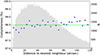 |
Fig. 1. Redshift completeness of the three equatorial GAMA regions G09, G12, and G15 as a function of the distance to the nearest neighbour among main survey targets (blue dots). As in Liske et al. (2015), the horizontal green line and the grey shaded histogram show the overall average redshift completeness and the distribution of all nearest neighbour distances, respectively. |
In the rest of this section, we describe the various GAMA data products that we make use of in our work. These include stellar masses (Sect. 2.1), the group catalogue (Sect. 2.2) and the filament catalogue (Sect. 2.3).
2.1. Stellar masses
For the stellar mass measurements and uncertainties we make use of the table StellarMassesLambdarv24 (Taylor et al. 2011), which provides stellar masses, restframe photometry, and other ancillary stellar population parameters from stellar population fits to multi-band spectral energy distributions for all objects across the five GAMA survey regions. The values in this catalogue were derived using a ‘737’ cosmology and distances that were computed using the flow-corrected redshifts derived from the Tonry et al. (2000) flow model for very low redshifts, and then tapering to a CMB-centric frame for z > 0.03, as described by Baldry et al. (2012). The broadband photometry that was modelled to derive the stellar masses (in the restframe wavelength range of 0.3–1.1 μm) is the 21-band matched aperture photometry presented by Wright et al. (2016, and published in the table LambdarCatv01). We corrected the masses derived from this aperture photometry for the light lying outside of the apertures as described by Taylor et al. (2011). However, following the approach of Vázquez-Mata et al. (2020), we only applied this correction if the correction factor is in the range 0.8–10; otherwise, no correction is applied. We note that we repeated our analyses with different limits for the correction factor and found that our results do not change qualitatively.
We point out that since the inception of the present work, the GAMA collaboration has updated both their preferred multi-band photometry [now derived using the code PROFOUND (Robotham et al. 2018) and published by Bellstedt et al. (2020)] as well as their preferred method of deriving stellar masses [now using the code PROSPECT (Robotham et al. 2020)]. As shown by Robotham et al. (2020), the joint net effect of these changes is a global shift of the stellar masses by +0.1 dex (with a scatter of 0.11 dex), approximately independent of stellar mass. This shift is of course irrelevant when performing purely internal comparisons of the GSMF as a function of different environmental properties (Sect. 6) but should be kept in mind when comparing our GSMF to literature values (Sect. 7).
2.2. Group catalogue
The GAMA galaxy group catalogue (G3C)2 is one of the major data products of the GAMA project (Robotham et al. 2011). The G3C was constructed by employing a modified Friends-of-Friends (FoF) grouping algorithm that considers galaxies to be in a group if they are ‘close’ both along the line of sight and when projected on to the sky; this successfully accounts for redshift space distortions caused by the peculiar velocities of galaxies in groups. This FoF algorithm was first run on mock GAMA light cones in order to tune the grouping parameters and to test the quality of the grouping, before applying it to the real GAMA data.
In particular, we make use of the following tables: (i) G3CGalv083, which lists the 184 081 galaxies on which the FoF algorithm was run. The exact selection of these galaxies is given by: nQ ≥ 2, SURVEY_CLASS ≥ 4, and 0.003 < zCMB < 0.6 (Baldry et al. 2012), as taken from the tables TilingCatv46 and DistancesFramesv14. (ii) G3CFoFGroupv093, which lists the properties of the 23 654 groups comprising 2 or more members that were identified among the galaxy sample above and which contain ∼40% of these galaxies.
2.3. Filament catalogue
The filament catalogue (FC)4 identifies the LSS in the three equatorial survey regions (Alpaslan et al. 2014). Using a volume-limited subsample of the G3C with a redshift cut of z ≤ 0.213 and an absolute magnitude cut of Mr = −19.77 + 5log h100, and discarding all groups with fewer than two members remaining after these cuts, Alpaslan et al. (2014) used the remaining groups as nodes to generate a minimal spanning tree, thus identifying 643 individual filaments spanned by 5152 groups. The 45 468 galaxies of their subsample were then classified as belonging to filaments, tendrils, or voids. However, since we do not want to restrict our analysis to this volume-limited subsample, we do not make use of these classifications here. Instead, we only use the group-defined filaments and make use of our own environmental classification as described in Sect. 4.1.
The filaments identified in this catalogue are composed of an average of eight groups and span up to  Mpc. In particular, groups in filaments are connected through straight lines called links. All groups that are in the same set of unbroken links are considered to be part of the same filament. Additional substructures are defined within a filament. The backbone refers to the combination of the two paths with the most links that begin from the edges of the filament and meet at its centre, defined as the group which is furthest away from all edges. In other words, the backbone is the longest path that travels from one end of a filament to the other through its most central group. All other paths that are connected to the backbone are referred to as branches, and their order determines how close they are to the backbone. A branch of order n always connects to a branch of order n − 1, which connects to a branch of order n − 2, and so on, where the backbone is considered a branch of order 1.
3. Sample selection
In this section we describe the selection defining our parent sample of galaxies. The final selection, which results from the application of the redshift-dependent stellar mass limit, is described in Sect. 5.2.
The spectroscopic GAMA observations targeted objects with dust-corrected Petrosian SDSS Data Release 7 (DR7) r-band magnitudes of r < 19.8 mag (Baldry et al. 2010). The reference table TilingCatv46 defines the class of each survey target (SURVEY_CLASS) as well as various redshift quality parameters (nQ and nQ2_FLAG, which records the result of tests of nQ = 2 redshifts against independent measurements). Our initial sample selection was defined as follows:
-
(i)
Survey regions G09, G12, and G15;
-
(ii)
r < 19.8 mag;
-
(iii)
SURVEY_CLASS ≥ 4 to select only main survey targets, excluding additional filler targets from the sample;
-
(iv)
nQ ≥ 3 or (nQ = 2 and nQ2_FLAG ≥ 1) to select targets with reliable redshifts.
Next, because we make use of the filaments identified by the FC, we applied the same upper redshift cut of z = 0.213. Because the various GAMA data products above used slightly different versions of the redshift data (i.e. TilingCatv46), small inconsistencies arose between these data products. As a result, our sample does not include one FC group because it was left with no members after our selection criteria were applied. Furthermore, 1088 galaxies catalogued in the G3C with nQ = 2 are not included in our sample because of our additional requirement of nQ2FLAG ≥ 1 (see above). We note that the redshift cut applied above is based on different measurements: For ungrouped galaxies, we considered the CMB frame redshift zCMB coming from the table DistanceFramev14; for a grouped galaxy, we just took the median redshift zFOF of the galaxy’s group coming from G3CFoFGroupv09. Therefore, either all or none of the galaxies in a group are considered as being part of our sample.
In Fig. 2 we show the distribution of the absolute r-band magnitude as a function of redshift for all the galaxies in G3CGalv08 (black dots), with the red dots highlighting our parent galaxy sample after our initial selection criteria were applied. To determine the faintest possible galaxy that is visible in GAMA at each redshift (shown as a magenta curve in Fig. 2), we first calculated the distance modulus DM as a function of redshift using the cosmological luminosity distance DL (in units of  Mpc):
Mpc):
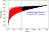 |
Fig. 2. Distribution of the absolute r-band magnitude as a function of redshift for all the galaxies in G3CGalv08 (black points). The magenta curve represents our selection function and gives the faintest possible galaxy that is visible in GAMA at each redshift, given our apparent magnitude limit of r = 19.8 mag. Red points show our parent galaxy sample after our initial selection criteria were applied. The two dashed green lines determine our redshift limits (see Sect. 3.1.2 for a discussion of the lower redshift cut). The dashed blue line shows the absolute magnitude cut applied by Alpaslan et al. (2014). |
 (1)
(1)
with DL = (1 + z)R0Sk(r). Here, R0Sk(r) refers to the radial comoving distance. We then calculated the absolute magnitude of the faintest possible galaxy that can be seen within the GAMA survey given our apparent magnitude limit of r = 19.8 mag and using the k-correction from Robotham et al. (2011) as
 (2)
(2)
This equation describes our initial selection function, that is, a function that precisely bounds our parent sample data. Unlike Alpaslan et al. (2014), we decided not to apply an absolute magnitude cut here in order to be able to probe the GSMFs more deeply. Our parent galaxy sample now contains a total of 89 451 galaxies across G09, G12, and G15 and 11 820 groups, 5151 of which are part of a filament.
We note that some black dots in Fig. 2 are actually still present below the upper redshift cut: these galaxies have nQ = 2 and nQ2_FLAG = 0. Also, some red dots lie above the same cut. These 69 galaxies have higher redshifts than 0.213 but belong to a group with a median redshift below this value. According to our selection process, the reverse is also possible but less clear from the plot. Fifty-two galaxies are not included in our final sample, even though they meet all the other requirements, because the group they belong to has a median redshift higher than 0.213.
In the rest of this section we now describe two small additional restrictions that have to be applied to our sample.
3.1. Additional sample selection
3.1.1. Stellar mass availability
A small mismatch of 45 galaxies between our spectroscopic and the available stellar mass sample described in Sect. 2.1, due to different selection processes, reduces our sample to 89 406 galaxies. Furthermore, the stellar mass catalogue provides the Posterior Predictive P-value (PPP) as a goodness of fit statistic, which can be roughly thought of as a Bayesian analogue to the frequentist reduced χ2. The PPP is a useful tool for checking whether or to what extent the model is consistent with the data. Given the observed data and the posterior probability density function on the properties of the model, the PPP quantifies the fraction of future observations that would be predicted to be as discrepant as the observed data. Here, we impose a lower limit of PPP ≥ 0.01 to discard those galaxies where the data invalidate even the ‘most likely’ model at 99% confidence. After the PPP cut, our galaxy sample consists of 88 581 objects.
3.1.2. Lower redshift limit
The three panels of Fig. 3 show the distribution of our groups in the filaments across the three GAMA equatorial fields. As one can see, no filament is found at redshifts z < 0.02. Below this redshift, the volume is simply not large enough to accommodate a typical filament, and the environment of a galaxy cannot be reliably determined. We thus imposed a lower redshift limit of z = 0.02 on our sample (Fig. 2, left dashed green line), in addition to the upper limit of z = 0.213 already applied above. Our final parent sample thus consists of a total of 88 093 galaxies and 11 725 groups, 5142 of which are part of a filament.
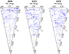 |
Fig. 3. Light cones of the three GAMA equatorial survey regions showing our FC group sample out to z = 0.213 (blue dots). All three cones span the full 5° declination range. |
We summarise the complete selection process of the parent sample in Table 1. The final step of the selection process, that is, the application of the redshift-dependent stellar mass limit, is described in Sect. 5.2.
Our parent sample selection process.
4. Environmental properties
In this section, we present four different environmental properties we make use of in this work. These are the orthogonal distance to the nearest filament D⊥,min (Sect. 4.1), group membership (Sect. 4.2), group halo mass Mhalo (Sect. 4.3), and a combination of the group’s branch order (BO) and the group’s number of connecting links (Nlinks; Sect. 4.4).
4.1. Orthogonal distance to nearest filament
As discussed in Sect. 2.3, from Alpaslan et al. (2014) we only use the filaments identified in the FC but we do not use their galaxy environmental classification. Therefore, we provided our own classification of whether a galaxy is part of a filament or a void, which is simply based on the distance of a galaxy to the nearest filament. In particular, for each galaxy we consider the orthogonal distance to its nearest filament, D⊥,min, as our first environmental measure. Our sample consists of 88 093 galaxies, 39 341 of which are assigned to a group and 48 752 of which are ungrouped (U subsample hereafter); of the grouped galaxies, 23 657 galaxies belong to groups in filaments (G1 subsample hereafter) and the remaining 15 684 galaxies to groups which are not part of a filament (G2 subsample hereafter). All galaxies in G1 were assigned D⊥,min = 0 Mpc by definition. For galaxies in U and G2, we first calculated their 3D Cartesian coordinates and then determined the values of D⊥,min. We note that to diminish the effects of redshift space distortions in this step of the process, the Cartesian coordinates of galaxies in G2 belonging to the same group were derived using the RA and Dec values of the iterative central galaxy as well as the median redshift of the group as stated in Sect. 3; in this way, all galaxies in a given group ended up with the same Cartesian coordinates. In Fig. 4 we show the distribution of D⊥,min for our galaxy sample. As expected, this distribution peaks at  Mpc and then decreases exponentially. The galaxies in G1 are responsible for the bump at D⊥,min = 0 Mpc.
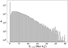 |
Fig. 4. Distribution of the orthogonal distance of a galaxy to its nearest filament. The galaxies in subsample G1 (galaxies in groups that are part of a filament) are responsible for the bump at 0 Mpc since they are assigned a value of D⊥,min = 0 Mpc by definition. |
4.2. Group membership
A galaxy’s membership of a group or not, as defined by the G3C in Sect. 2.2, represents our second environmental property. As described above, this categorical classification comprises 39 341 grouped galaxies (G1 + G2 subsamples) and 48 752 ungrouped galaxies (U subsample).
4.3. Group halo mass
As in Vázquez-Mata et al. (2020), we make use of two different methods for estimating a group’s halo mass Mhalo, which represents our third environmental measure. The first method provides a dynamical mass estimate, Mdyn, based on the virial theorem and the galaxy dynamics within each group; the second provides a luminosity-based mass estimate, Mlum, using the group’s total r-band luminosity and the weak-lensing calibrated M–L relation of Viola et al. (2015, Eq. (37)). As discussed in Robotham et al. (2011), the total group r-band luminosity is not simply the sum of the luminosities of all galaxies belonging to that group, but is instead corrected for the fraction of light in galaxies below the survey magnitude limit using the global GAMA luminosity function. Since most of the luminosity is contributed by galaxies around L⋆, and since most GAMA groups are sampled well beyond L⋆ due to the survey’s depth of r < 19.8 mag, these corrections typically amount to only a few percent.
The G3C provides the dynamical group halo masses, both using a constant calibration factor of A = 10.0 required to get a median unbiased mass estimate (column MassA), as well as using a calibration factor that is a function of group multiplicity and redshift (column MassAfunc). Also listed are the group r-band luminosities integrated down to an absolute magnitude of Mr − 5log h100 = −14, again both considering a constant calibration factor of B = 1.04 for the median unbiased luminosity estimate (LumB), and its functional form (LumBfunc). See Sects. 4.3 and 4.4 of Robotham et al. (2011) for detailed explanations of these different calibration factors.
In Fig. 5 we show the halo mass distribution of our group sample using both the dynamical estimate (black dashed line) and the luminosity-based one (solid line). Our groups mainly reside in halos of  . Moreover, the dynamical mass estimates have a broader distribution towards lower masses compared to the luminosity-based ones, as already noted by Han et al. (2015) and Vázquez-Mata et al. (2020). We also show as blue and red dashed lines the dynamical halo mass distributions of the groups that define the filaments and those that lie outside of the filaments. Although there is an almost complete overlap, these distributions are nevertheless quite different, with the groups in filaments clearly being more massive. In fact, the group sample is dominated by the filament groups at halo masses
  , and by the groups outside of filaments below that value.
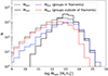 |
Fig. 5. Black solid and dashed lines show the distributions of the luminosity-based and dynamical halo mass estimates for our group sample, respectively. The blue and red dashed lines show the distributions of the dynamical halo mass estimates for those groups that are part of a filament and those that are not, respectively. |
4.4. Group branch order and number of connecting links
In the FC, 656 filaments spanned by 5152 groups were identified across the three equatorial GAMA regions. As explained in Sect. 2.3, a filament is defined as a collection of branches. Each branch (and therefore each group within a branch as well as each galaxy within those groups) can be assigned a branch order (BO). In particular, groups with BO = 1 define the backbone; groups with BO = 2 belong to a second-order branch (connected to the backbone); and so on. The backbone and all the other branches of a filament make up its morphology, with the backbone representing the most central route through the filament, and the other branches being paths that emerge from the backbone.
Apart from the order of its branch, the position of a group within its filament can be further characterised by its total number of links to neighbouring groups, Nlinks. A group at the end of its branch has Nlinks = 1, a group in the middle of a branch has Nlinks = 2, while a group belonging to multiple branches has Nlinks > 2. To obtain a comprehensive picture of how much a group is embedded in a denser (or less dense) part of a filament, we consider both its BO and its Nlinks, the combination of which represent our final environmental property.
5. Method
In this section we describe the methods we used in our work: the Modified Maximum Likelihood estimator for the construction of the GSMFs (Sect. 5.1), the stellar mass completeness limit for the derivation of the selection function (Sect. 5.2) and the random sample generation for the application of volume corrections to the GSMFs (Sect. 5.3).
5.1. Modified maximum likelihood estimator
Massive galaxies are much rarer compared to low-mass ones. In a fixed cosmic volume, the number of galaxies per unit mass decreases with mass according to a power law until reaching a specific cut-off, beyond which the number density falls off exponentially. To characterise this behaviour, it is helpful to define the GSMF ϕ(M) as the density of galaxies per unit volume and per unit stellar mass M. Specifically, in a given cosmic volume dV, the expected number of galaxies within the interval [M, M + dM] is given by dN = ϕ(M)dVdM. Analytical parametric functions intended to match observed GSMFs can be expressed in the form ϕ(M|θ), where θ denotes a vector of P scalar model parameters. The Schechter function (Schechter 1976) represents the most well-known model accurately capturing the truncated power-law behaviour:
 (3)
(3)
Here, ϕ⋆ is the normalisation factor, M⋆ is the mass at the normalisation point (i.e. near the exponential break), and α is the faint-end slope parameter. However, the shape of the GSMF is not always well represented by a single Schechter function due to an often observed steepening below 1010 M⊙, giving rise to a double Schechter function (Baldry et al. 2008):
 (4)
(4)
where  ,
,  and α1, α2 describe the normalisation and slope parameters, respectively, for the two components. Without loss of generality, we can always choose α1 > α2 such that the second term in Eq. (4) dominates at lower masses (Baldry et al. 2012).
The most straightforward and intuitive technique for fitting a GSMF model, as described in Schmidt (1968), is to estimate the observed space densities for different mass intervals of the data. This is achieved by computing for each mass interval the ratio between the number of detected galaxies and the maximum volume Vmax in which galaxies of that mass could have been observed. This procedure is also known as 1/Vmax method. The model function ϕ(M|θ) is then fitted to these values. However, this method has several drawbacks: the fitting process is influenced by the division into arbitrary mass intervals; Poisson errors cannot be assigned to non-detections (i.e. mass intervals with no galaxy); the choice of Vmax is sometimes uncertain due to complex detection limits with source-dependent completeness; and systematic errors can be introduced by the cosmic LSS. Just observing more galaxies will not solve most of these limitations, which indeed remain a pertinent issue for modern spectroscopic redshift surveys.
In this study, we hence employ the modified maximum likelihood (MML) estimation, which was comprehensively documented by Obreschkow et al. (2018). This method bypasses the need for data binning and operates within a Bayesian framework tailored for fitting distribution functions (e.g. GSMFs) to complex multi-dimensional datasets. The MML framework meticulously takes into account the observational measurement errors for individual objects, incorporates complex observational selection functions, and provides the option to internally correct for the underlying LSS detected within the survey volume. The core of the MML approach consists of a fit-and-debias procedure, an iterative fitting algorithm that iteratively solves a standard maximum likelihood estimation, revising the data by accounting for the previous fit and observational uncertainties. The MML framework is accessible via DFTOOLS (Obreschkow et al. 2018), an open-source software package for the R statistical programming language. DFTOOLS gives the most likely solution and full co-variance matrix of the relevant model parameters in order to derive volume-corrected binned mass functions. In our analysis, we fit a double Schechter function (Eq. (4)), which has been demonstrated to effectively address the notable upturn observed at intermediate stellar masses (Baldry et al. 2008).
5.2. Stellar mass completeness limit
One of the most crucial steps in properly estimating the number density ϕ(M) consists in the derivation of Mlim(z), which represents the stellar mass limit above which our sample is complete at a given redshift, and which depends both on redshift and the stellar mass-to-light M/L distribution of the sample, given our flux-limited sample.
The determination of the stellar mass completeness limit is particularly challenging for a flux-limited sample like ours, since a sharp limit in luminosity does not correspond to a sharp limit in stellar mass, as shown in Fig. 6. Taking a narrow redshift range (dashed black lines, left-hand panel) and simply using as a mass limit (solid green line, right-hand panel) the mass that corresponds to the luminosity limit and the average M/L (respectively, solid blue and dashed cyan line, right-hand panel) would result in an incomplete sample, since all the massive yet lower-luminous sources falling below the absolute magnitude cutoff are already missing from the sample. Therefore, it is necessary to move the mass limit sufficiently upwards (dashed green line, right-hand panel) to reduce the incompleteness to an acceptable level.
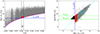 |
Fig. 6. Left-hand panel: Distribution of the total r-band luminosity as a function of redshift for our parent galaxy sample (grey dots). The magenta curve represents our selection function and gives the lowest luminosity of a galaxy for which a redshift could have been collected in GAMA, given our apparent magnitude limit of r = 19.8 mag. The two dashed black lines define a narrow redshift range Δz for illustrative purposes. The solid blue line and the red box correspond to the luminosity limit and the 20% faintest galaxies associated with this redshift range, respectively. Right-hand panel: Stellar mass versus r-band luminosity for the galaxy subsample in the narrow redshift range, Δz, defined in the left-hand panel. The dashed cyan line gives the average correlation between the two galactic properties. Galaxies lying above this line have a higher than average M/Lr and vice versa. The luminosity limit from the left-hand panel is also shown here in blue. The intersection of this limit with the average correlation defines the corresponding mass limit at this redshift shown as a solid green line. However, this mass limit would not in fact result in a complete sample as all galaxies to the left of the blue line, shown in black, would be missed. To be complete, it is necessary to move the mass limit up sufficiently such that (almost) no more galaxies are missed. The dashed green line thus gives the final stellar mass limit, representing the 95% M/Lr completeness limit of the 20% faintest galaxies at this redshift (see text). |
Different strategies for the estimation of Mlim(z) can be found in the literature. For example, the approach presented in Dickinson et al. (2003), Fontana et al. (2006), Pérez-González et al. (2008) and others rely on a single stellar population (SSP) paradigm; the minimum stellar mass of a galaxy with magnitude equal to the magnitude limit rlim can be estimated by scaling the flux of a synthetised spectrum of a passively evolving SSP formed at high redshift. The technique introduced by Marchesini et al. (2009) considers deeper survey data, where the flux and mass of each object are scaled to match rlim; in this context, the most massive sources have the lowest M/L and can therefore be excluded by simply applying rlim as a cut. Quadri et al. (2012) and Tomczak et al. (2014) use a slightly modified version of this approach, by considering the objects above the flux completeness and scaling their masses and fluxes down to rlim; the upper limit of those scaled-mass values defines their mass completeness limit as a function of redshift.
In this work, we followed the approach presented by Pozzetti et al. (2010) and illustrated in Fig. 7. For each galaxy in our sample, we first considered Mlim, i, that is, the mass that source i would have if it had the same M/Lr but a magnitude equal to our spectroscopic magnitude limit of rlim = 19.8 mag. In Fig. 7 we show the resulting distribution in Mlim, i which reflects that of the Mi/Lr, i at each redshift in our sample. In other words, Mlim, i is M/Lr dependent. Under the assumption of a constant M/Lr, Mlim, i is simply given by
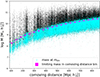 |
Fig. 7. Determination of the stellar mass completeness limit as a function of comoving distance for our galaxy sample (black dots). Due to the range in M/Lr, constraining the mass completeness limit of a flux limited sample is not straightforward. By keeping the M/Lr and the redshift of each source constant, we determined the stellar mass that each object would have if its flux was equal to the flux limit. These limiting mass values are shown in cyan, with higher dots at a given redshift having larger M/Lr values. We then divided our sample into bins of comoving distance, sorted the sources in each bin according to their luminosity, selected the faintest 20%, and determined the stellar mass below which 95% of these faint objects lie (Pozzetti et al. 2010). We repeated this procedure for each bin and thus obtained the limiting mass values that are shown as magenta squares. The mass completeness function Mlim(d), shown as the magenta dashed line, was then estimated by fitting an exponential curve to these limiting mass value in each comoving distance bin. |
 (5)
(5)
Next, we divided our sample into 20 bins of comoving distance d and then, in each bin, sorted all sources by magnitude, selecting the 20% faintest galaxies (shown in red in Fig. 6). For each bin, we defined Mlim as the upper envelope of the Mlim, i distribution, below which 95% of these faint objects lie. The function Mlim(d) was then determined by fitting an exponential curve to the estimated mass limits in each bin defined as
![Mathematical equation: $$ \begin{aligned} \log [M_{\rm lim} / (M_\odot \,h_{70}^{-2})] (d) = a \log [d / (\mathrm{Mpc}\,h_{70}^{-1})] + b, \end{aligned} $$](/articles/aa/full_html/2025/04/aa53570-24/aa53570-24-eq14.gif) (6)
(6)
with a and b being the free parameters. The fit resulted in a = 1.0668 and b = 3.1956. This Mlim(d) therefore corresponds to the 95% completeness limit of the M/Lr distribution of the 20% lowest-luminosity galaxies at each redshift and represents the selection function for our sample (shown as the magenta dashed line in Fig. 7).
Unavoidably, however, the (small) remaining incompleteness of the sample thus selected is not random. Instead, it depends on luminosity and M/Lr, with faint, high-M/Lr galaxies most affected. Since any subsample of galaxies that we might choose to select below may have an Lr-M/Lr distribution that is slightly different from that of the full sample (at a given redshift), the incompleteness of this subsample will also be slightly different from that of the full sample. This could be avoided by re-determining Mlim individually for each subsample. However, this would result in the union of a complete set of subsamples not necessarily being identical to the full sample, and these subsamples covering slightly different volumes, which may in turn result in slightly different LSS corrections. In practice, however, we found that the two methods produce essentially the same results for all of our subsamples. For simplicity, we hence use the same selection function for all subsamples.
Finally, we amended our selection function at the lowest redshifts by requiring ![Mathematical equation: $ \log [M / (M_\odot \, h_{70}^{-1})] > 8.3 $](/articles/aa/full_html/2025/04/aa53570-24/aa53570-24-eq15.gif) (cf. Fig. 7) because we found our mass function measurements below this value to be unreliable for many of the subsamples that we investigate in Sect. 6 below.
(cf. Fig. 7) because we found our mass function measurements below this value to be unreliable for many of the subsamples that we investigate in Sect. 6 below.
At this point, the sample was restricted to the galaxies that lie above this curve. This resulted in our final sample of 52 089 galaxies (59% of the parent sample defined in Sect. 3) and 10 429 groups. We note that when referring to any subsamples below, in particular the samples G1, G2 and U defined in Sect. 4.1 above, these samples should be understood to have had the selection function shown in Fig. 7 applied to them.
To measure a given sample’s GSMF, we input the selected galaxies’ comoving distances, stellar masses, stellar mass errors, selection function, and desired functional form to fit (i.e. double Schechter) into the DFTOOLS routine DFFIT. We note that the code computes both the functional fit as well as the full covariance matrix for the fitted parameters.
5.3. Random sample generation
The general mass function of filament galaxies just considers all the galaxies in filaments, using the total survey volume, and describes the overall average density of galaxies living in filaments. In contrast, the ‘conditional’ GSMF (cGSMF hereafter) represents the local density of galaxies in filaments, given that they are a member of a filament. To see how the local density of galaxies changes as a function of environment, we need to know which fraction of the total survey volume is occupied by filaments (assuming a certain radius) and voids. To this end, we distribute a random sample of points in the total survey volume and then ask which fraction of this sample lies within various environments. The density of this random sample is determined by the requirement to have the volume of a sphere with the minimum filament radius considered in our analysis (i.e. 3 Mpc  ), probed by at least 30 random points. This leads us to a total number of ∼3 billion random points spread across the three equatorial regions.
In Table 2 we provide the fractional volumes of both filaments and voids as a function of filament radius. We note that Alpaslan et al. (2014) used a radius of 4.13 Mpc  to divide galaxies into filament and void galaxies in the FC.
Fraction of the total survey volume occupied by filaments and voids (i.e. everything outside the filaments) as a function of the assumed filament radius.
Best-fit double Schechter function parameters for the mass functions in voids (left) and filaments (right), when considering our entire galaxy sample.
6. Results
In this section we present our results on the variation of the cGSMF as a function of each environmental property described in Sect. 4: orthogonal distance to the nearest filament D⊥,min (Sect. 6.1), group membership (Sect. 6.2), group halo mass Mhalo (in particular, its dynamical estimate Mdyn in Sect. 6.3.1 and its luminosity-based one Mlum in Sect. 6.3.2), and the combination of group branch order BO and group number of connecting links Nlinks (Sect. 6.4).
6.1. How the GSMF differs in filaments and voids
We now investigate the cGSMF in filaments and in voids. As discussed in Sect. 2.3, we use the definition of the quasi one-dimensional filaments identified in the equatorial GAMA regions by Alpaslan et al. (2014), but we do not use their classification of galaxies as belonging to filaments or voids. Instead, we prefer to implement our own classification in order to be able to investigate the effect of assuming different filament radii. Since we do not know a priori how thick a typical filament should be, we used different filament radii, as listed in Table 2. Having calculated, for each galaxy in our sample, its orthogonal distance to the nearest filament, D⊥,min, we consider all galaxies with D⊥,min smaller than the filament radius under consideration as being part of a filament, while all others are considered void galaxies.
In Fig. 8(a) we show the cGSMFs of void and filament galaxies as a function of the filament radius. Their best-fit double Schechter function parameters are tabulated in Table 3 and shown in Fig. 9(a). We note that in these and similar tables and figures throughout this paper, we only present our results regarding M⋆, α1 and α2 since we are more interested in any change of the shape of the mass function and less in its normalisation. From Figs. 8(a) and 9(a) we see that the shape of the void GSMF is essentially unaffected by the filament radius. On the other hand, the filament GSMF does show some small variation in M⋆. However, by far the most striking feature of these figures is the very significant difference in the shapes of the filament and void GSMFs, which is manifested in all three of the Schechter function parameters shown.
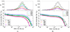 |
Fig. 8. Lower panels: cGSMFs in voids and filaments colour-coded by filament radius (as indicated in the legend). In panel (a), we use our entire galaxy sample, while in panel (b) we discard all the grouped galaxies from our filament samples. Our global GSMF is also shown in black. Upper panels: Raw number of galaxies as a function of stellar mass in each sample, as indicated. |
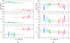 |
Fig. 9. Best-fit double Schechter function parameters of the cGSMFs shown in Fig. 8 using the same colour-coding by filament radius. The differences between filaments and voids found for M⋆, α1, and α2 when using the entire galaxy sample in panel (a) vanish after removing all grouped galaxies from the filament samples in panel (b). We note the different scaling of the y-axes in (a) and (b). |
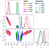 |
Fig. 10. Likelihood contours at the 1σ, 2σ, and 3σ levels of the cGSMFs in voids and filaments colour-coded by filament radius as indicated in the legend. For each distribution, 105 random samples were generated. |
In Fig. 10 we show the 1σ, 2σ and 3σ likelihood contours of the cGSMFs in voids and filaments. Clearly, the differences in the double Schechter function parameters M⋆, α1 and α2 between voids and filaments, already seen in Fig. 9(a), remain significant when taking into account the correlations among the parameters.
So far, we have only considered the cumulative (w.r.t. filament radius) mass functions. In Fig. 11 we now show the Schechter function parameters of the cGSMFs in differential bins of D⊥,min. This clearly demonstrates that the difference between the shapes of the void and filament cGSMFs is entirely driven by the innermost 0–3 Mpc  bin. In fact, as we subsequently demonstrate, it is entirely driven by the galaxies belonging to the groups that define the filaments.
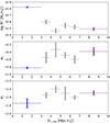 |
Fig. 11. Best-fit double Schechter function parameters for the differential cGSMFs in the range 3–7 Mpc |


In Sect. 4.1 we defined the G1 subsample as all those grouped galaxies for which the groups are part of a filament. These galaxies were assigned D⊥,min = 0 by definition. We now discard the G1 subsample from our filament samples. The new cGSMFs as a function of the filament radius are shown in Fig. 8(b), and their best-fit double Schechter function parameters are tabulated in Table 4 and shown in Fig. 9(b). With the removal of the grouped galaxies from our filament samples, the differences between the shapes of the void and the filament cGSMFs have disappeared almost entirely, as shown in Fig. 8(b). In particular, the new filament cGSMFs now have systematically lower M⋆ and shallower α1 and α2 values, almost indistinguishable from those of the void mass functions. In other words, the galaxies in G1 contribute significantly to higher masses and steeper slopes, leading us to conclude that the shape of the GSMF is not strongly affected by the larger-scale environment (i.e. voids versus filaments), but rather by group membership.
6.2. How the GSMF differs for grouped and ungrouped galaxies
We now demonstrate the effect of group membership on the mass function explicitly by directly comparing the cGSMFs of grouped and ungrouped galaxies.
The volume correction for the group galaxy sample was calculated as follows. First, each group was assigned the median Rad50 of the groups with the same number of members, where Rad50 is the group radius defined by the 50th percentile group member (taken from the G3C). The group’s volume was then calculated assuming a spherical shape, and the final volume correction was then derived by summing up the volumes of all groups. When we divide our sample into bins of a group property, as we do in Sects. 6.3 and 6.4, each volume correction is derived by summing up the volumes of those groups with the property within that bin.
Our resulting cGSMFs are shown in Fig. 12, and the best-fit double Schechter function parameters are tabulated in Table 5 (cf. also Fig. 14). Clearly, the mass functions of the grouped (in yellow) and ungrouped galaxies (in brown) differ substantially: the characteristic mass M⋆ of the grouped cGSMF is larger, its intermediate-mass slope α1 is steeper, while its low-mass slope α2 is essentially the same. As we shall see in the next subsection, these differences are likely due to the ungrouped galaxies being hosted by less massive halos compared to the grouped galaxies.
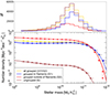 |
Fig. 12. Lower panel: cGSMFs of grouped and ungrouped galaxies, as indicated in the legend. The grouped galaxies have further been subdivided into those that are part of a filament and those that are not. We note that our total group sample occupies a volume of just ∼2.4 × 10² Mpc |

Best-fit double Schechter function parameters for the mass functions of grouped and ungrouped galaxies.
Splitting the group galaxy sample into those that are part of a filament (subsample G1) and those that are not (subsample G2), we also find significant differences. In particular, the cGSMF of the grouped filament galaxies has a larger characteristic mass than that of the grouped galaxies outside of filaments. Again anticipating the results of the next subsection, we attribute this difference to the larger halo masses of the filament groups compared to the groups outside of filaments, as shown in Fig. 5.
We also note the large difference in the normalisation of the grouped and ungrouped cGSMFs by ∼4 orders of magnitude. This is of course due to the cGSMFs effectively measuring the typical local density in groups and of ungrouped galaxies. While the raw numbers of grouped and ungrouped galaxies in our sample are actually quite similar (cf. Sect. 4.2 and upper panel of Fig. 12), the volumes occupied by them are vastly different, generating the large difference in density. We hasten to point out, though, that our method of determining the volume occupied by the groups is only very approximate.
Having established the group environment as an important factor in shaping the GSMF, we now turn to investigating the GSMF as a function of group properties.
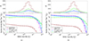 |
Fig. 13. Lower panels: cGSMFs of the group galaxy subsample colour-coded by Mdyn as indicated in the legend. In panel (a), we use the MassA calibration factor, while in panel (b) we use the MassAfunc factor. For comparison, the cGSMF of the ungrouped galaxies is also shown in brown. Upper panels: Raw number of galaxies as a function of stellar mass in each sample, as indicated. |
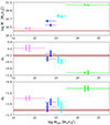 |
Fig. 14. Best-fit double Schechter function parameters of the cGSMFs shown in Fig. 13 using the same colour-coding by Mdyn. For clarity, the vertical error bars corresponding to the MassA estimator have been slightly offset to the left. The brown horizontal bands show the results for the ungrouped galaxy sample. |
6.3. GSMF dependence on group halo mass
In this section, we study the dependence of the GSMF on group halo mass Mhalo. As described in Sect. 4.3, we have two different estimates of Mhalo: the dynamical mass estimate Mdyn and the group r-band luminosity-based mass estimate Mlum. We now describe our GSMF measurements using these two estimates in turn.
6.3.1. GSMF dependence on dynamical group halo mass
To study the dependence of the GSMF on dynamical group halo mass Mdyn, we are forced to discard 879/10 429 (8.4%) of our groups for which the G3C does not report any Mdyn values because the measured velocity dispersion of these groups is smaller than its error. These are overwhelmingly groups with NFOF = 2. Our total sample now consists of 9550 groups containing 25 567 galaxies.
Next, we bin the galaxies into four different bins in ![Mathematical equation: $ \log [M_{\mathrm{dyn}} / (M_{\odot} \, h^{-1}_{70})] $](/articles/aa/full_html/2025/04/aa53570-24/aa53570-24-eq29.gif) according to the mass of the group that they belong to: ≤12.5, 12.5–13, 13–13.5, and > 13.5 (cf. Fig. 5).
according to the mass of the group that they belong to: ≤12.5, 12.5–13, 13–13.5, and > 13.5 (cf. Fig. 5).
As explained in Sect. 4.3, the G3C provides the dynamical group halo mass using two different calibration factors, which we refer to as MassA and MassAfunc, respectively.
Our resulting cGSMFs, colour-coded by Mdyn, are shown in Fig. 13(a) for the MassA calibration factor and in (b) for the MassAfunc factor, respectively. The best-fit double Schechter function parameters are tabulated in Table 6 and shown in Fig. 14. We first point out that the characteristic mass M⋆ clearly increases with Mdyn. In other words, more massive halos tend to host more massive galaxies, a result to be expected in a hierarchical structure formation paradigm, where larger halos form by the merging of smaller ones, accumulating more mass and forming larger central galaxies. Furthermore, the intermediate-mass slope α1 steepens with Mdyn, that is, a more rapid decline with stellar mass in the number of intermediate-mass galaxies is observed in more massive halos. In contrast, there is no evidence for any trend in the low-mass slope α2, except possibly for an increase in the highest halo mass bin, where the cGSMF is nonetheless best represented by a single Schechter function (with α2 = α1). Reassuringly, these results are largely robust against the choice of calibration factor.
Best-fit double Schechter function parameters of the cGSMFs of grouped galaxies for different subsamples, as indicated.
We also find that the results of the previous subsection are broadly consistent with these trends in that the differences between the shapes of the cGSMFs of grouped galaxies in filaments and those outside of filaments can be explained almost entirely by the fact that the halo masses of groups in filaments are systematically higher than those of groups outside of filaments (cf. Fig. 5). The only exception is the very steep low-mass slope of the grouped galaxies in filaments (cf. Table 5).
To investigate whether the shape of the cGSMF of the ungrouped galaxies also fits this picture we show in Fig. 14 (as brown lines) the best-fit double Schechter function parameters of the ungrouped galaxies derived in the previous subsection. Of course, for these galaxies we lack an estimate of their halo masses but it seems reasonable to assume that the halo mass distribution of these galaxies will be skewed towards similar or even lower masses than that of the group halos in our lowest halo mass bin. Under this assumption, at least the M⋆ value of the ungrouped galaxies is entirely consistent with the M⋆-halo mass trend of grouped galaxies.
Overall, we thus conclude that there is clear evidence of a dependence of M⋆ and α1 on halo mass, while there is no clear trend for α2.
6.3.2. GSMF dependence on luminosity-based group halo mass
To study the dependence of the GSMF on luminosity-based group halo mass Mlum, we follow the work of Vázquez-Mata et al. (2020) and only consider high-fidelity groups with multiplicity NFOF > 4 and  , as this is the sample for which the luminosity-halo mass scaling relation of Viola et al. (2015) is well calibrated. We are thus forced to discard 8917/10 429 (85.5%) of our groups, leaving us with 1512 groups containing 11 417 galaxies.
We now bin the remaining galaxies into three different bins in ![Mathematical equation: $ \log [M_{\mathrm{lum}} / (M_{\odot} \, h_{70}^{-1})] $](/articles/aa/full_html/2025/04/aa53570-24/aa53570-24-eq40.gif) according to the mass of the group that they belong to: ≤13.75, 13.75–14.25, and > 14.25 (cf. Fig. 5).
according to the mass of the group that they belong to: ≤13.75, 13.75–14.25, and > 14.25 (cf. Fig. 5).
As explained in Sect. 4.3, the G3C provides the total group luminosity that we use to derive the luminosity-based halo mass using two different calibration factors, which we refer to as (LumB) and (LumBfunc), respectively.
Our resulting cGSMFs, colour-coded by Mlum, are shown in Fig. 15(a) for the LumB calibration factor and in (b) for the LumBfunc factor, respectively. For a direct comparison, panels (c) and (d) show the corresponding cGSMFs for the same mass bins using the dynamical halo mass estimator (i.e. using Mdyn for the bin assignment, and using the same NFOF > 4 selection). The best-fit double Schechter function parameters are tabulated in Table 7 and shown in Fig. 16, where the left panels show the results for Mlum and the right panels those for Mdyn. We see that all four mass estimators provide results that are largely consistent with each other for all three Schechter function parameters. As in the previous subsection, we also find here that the cGSMF is best represented by a single Schechter function at  . However, with the cGSMFs of the intermediate and high halo mass bins being essentially identical, it is not possible to confidently confirm the trends with halo mass observed in the previous subsection with this more limited (albeit higher fidelity) sample. On the other hand, the results are not inconsistent with these trends either.
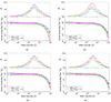 |
Fig. 15. Left column, lower panels: cGSMFs of our high-fidelity group galaxy subsample colour-coded by Mlum, as indicated in the legend. In panel (a) we use the LumB calibration factor, while in panel (b) we use the LumBfunc factor. Right column, lower panels: Same as the left but using the dynamical halo mas estimates with the MassA calibration factor in panel (c) and the MassAfunc factor in panel (d). Upper panels: Raw number of galaxies as a function of stellar mass in each sample, as indicated. |
Best-fit double Schechter function parameters of the cGSMFs of grouped galaxies for different subsamples, as indicated.
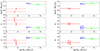 |
Fig. 16. Best-fit double Schechter function parameters of the cGSMFs shown in Fig. 15 using the same colour-coding by Mlum (left) or Mdyn (right). For clarity, the vertical error bars corresponding to the LumB (left) and MassA (right) estimators have been slightly offset to the left. |
6.4. GSMF dependence on group branch order and number of connecting links
In Sect. 6.1 we analysed the change (or lack thereof) of the mass function when moving perpendicularly to the filaments. We now investigate the dependence of the GSMF on the position within the filamentary structure.
From our groups-in-filaments galaxy subsample (G1) defined in Sect. 4.1, we select six different subsamples according to specific combinations of group branch order BO and group number of connecting links Nlinks, as listed in Table 8. In particular, we distinguish between galaxies in groups located in their filaments’ backbone (BO = 1) and in their outskirts (BO > 1), as well as between galaxies inhabiting groups located at the edge (Nlinks = 1), at an intermediate position (Nlinks = 2), and at the centre (Nlinks > 2) of their filament. We note that the full range of both parameters is 1–5.
Selection of 2 × 3 = 6 different subsamples from the FC group galaxy sample (G1) based on the group branch order (BO) and number of connecting links (Nlinks).
The resulting cGSMFs are shown in Fig. 17 as a function of the combination of BO and Nlinks. The best-fit double Schechter function parameters are tabulated in Table 9 and shown in Fig. 18. We first note that, when moving from the backbone (in red) to the outskirts (in blue), none of the three double Schechter parameters seem to vary very significantly, regardless of the value of Nlinks. Both for centres and edges, the backbone and outskirts are in excellent agreement in all three Schechter parameters, while for the intermediate regions some mildly significant differences appear, with higher M⋆ and α2 values and a lower α1 value in the outskirts compared to the backbone. However, this may be affected by the fact that the cGSMF of the intermediate regions in outskirts are best fit with a single Schechter function (where α1 = α2), which also applies to the central regions of both the backbone and the outskirts (cf. Table 9).
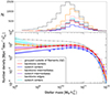 |
Fig. 17. Lower panel: cGSMFs of grouped galaxies in filaments (G1 subsample), colour-coded by a combination of BO and Nlinks as indicated in the legend. For comparison, the cGSMF of grouped galaxies outside of filaments (G2) is also shown in grey. Upper panel: Raw number of galaxies as a function of stellar mass in each sample, as indicated. |
Best-fit double Schechter function parameters for the mass functions of grouped galaxies in filaments for different subsamples and for grouped galaxies outside of filaments, as indicated.
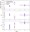 |
Fig. 18. Best-fit double Schechter function parameters of the cGSMFs shown in Fig. 17, as indicated in the legend. The grouped galaxies outside of filaments (in grey) are somewhat arbitrarily shown at Nlinks = 0. |
In addition, we did not find any significant trends as a function of Nlinks for any of the Schechter function parameters for the backbone or the outskirts sample, or their combination. This remains true if we add, somewhat arbitrarily, the Schechter function parameters of grouped galaxies outside of filaments at Nlinks = 0 (shown in grey in Fig. 18). All we observed here is that the M⋆ value of grouped galaxies outside of filaments is significantly lower that that of grouped galaxies in filaments, as we had already noted in Sect. 6.2.
We thus conclude that there is no evidence for any differences in the shape of the GSMF of grouped galaxies in filaments as a function of position within the filamentary structure.
7. Discussion
In this section we first compare our global GSMF with other GAMA and SDSS DR7 GSMFs (Sect. 7.1), and then discuss our results on the dependence of the mass function on different environmental measures in the context of other similar studies (Sect. 7.2).
7.1. Global GAMA and SDSS DR7 GSMFs
Many studies have already been undertaken inside the GAMA project concerning GSMFs. Baldry et al. (2012) selected a flux-limited sample of 5210 galaxies from the earliest phase of the GAMA project, called GAMA I, covering an area of 143 deg2. This sample was complete to r = 19.4 mag in the G09 and G15 regions and to r = 19.8 mag in G12, and covered the redshift range 0.002 < z < 0.06. Kelvin et al. (2014) selected a local volume-limited subsample of 2711 galaxies, also from GAMA I, to a lower stellar mass limit of M = 109 M⊙, covering 0.025 < z < 0.06. Similarly, Alpaslan et al. (2015) defined a local volume-limited subsample of 7195 galaxies to a lower stellar mass limit of M = 109.5 M⊙, up to z = 0.1. Wright et al. (2017) expanded the analysis by Baldry et al. (2012) to the full GAMA II dataset. Their flux-limited sample, covering the same GAMA II equatorial regions of 180 deg2 used in this study, was complete down to r = 19.8 mag and covered the redshift range 0.002 < z < 0.1. Baldry et al. (2012), Kelvin et al. (2014) and Wright et al. (2017) all computed their global GSMFs using a density-corrected 1/Vmax method. Completing the set of GSMF studied with GAMA, Driver et al. (2022) most recently considered a flux-limited sample of 13 957 galaxies from the latest version of GAMA, called GAMA III, adding the G23 region to the equatorial regions for a total area of 250 deg2. The magnitude limit of this sample was r = 19.65 mag, covering a redshift range of 0.0013 < z < 0.1. They computed their GSMF using the same MML estimator as in the present study. Finally, we include in our comparison the GSMF of Weigel et al. (2016), which was measured from a sample of ∼110 000 galaxies selected from the SDSS DR7, covering an area of 7748 deg2, with a magnitude limit of r = 17.77 mag and a redshift range of 0.02 < z < 0.06. Their GSMF was computed using the parametric maximum likelihood method, originally developed by Sandage et al. (1979).
The global GSMF was fit with a double Schechter function in almost all of theses studies. The only exception is Alpaslan et al. (2015) who used a single Schechter function. We list the best-fit Schechter parameters in Table 10 and compare the corresponding functions to our data and best-fit double Schechter function in Fig. 19. Evidently, our global GSMF, shown in black, is in very good agreement with all of the mass functions of the previous studies described above, except that of Alpaslan et al. (2015). The agreement is best with the GSMF of Driver et al. (2022), with the differences being less than a factor of two over the entire range of four orders of magnitude in stellar mass considered here (cf. lower panel of Fig. 19). The overall excellent agreement between these various mass functions is quite remarkable, given the differences in photometry, stellar mass estimation techniques, and GSMF measurement procedures.
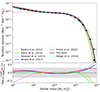 |
Fig. 19. Upper panel: Comparison of our global GSMF with other recent measurements derived from GAMA and SDSS data, as indicated. Lower panel: Logarithmic ratio of the literature GSMFs relative to ours. The grey shaded area indicates agreement within a factor of two. |
Nevertheless, some differences remain. At high stellar masses, the lower M⋆ values of the GAMA I studies by Baldry et al. (2012) and Kelvin et al. (2014) are likely due to the over-fragmentation of bright galaxies relative to fainter and smaller systems in the original GAMA aperture photometry, causing their fluxes to be underestimated and thus leading to an underestimate of their stellar masses as well. This issue was addressed in the photometry presented by Wright et al. (2017), which we have also used in this work. We note that our M⋆ value compares well with that of Driver et al. (2022) despite their use of further improved photometry and the improved stellar mass estimation technique of Robotham et al. (2020). At intermediate masses, where the inter-GSMF agreement is best, our global GSMF confirms a plateau from ∼109.5 to  , which was already noticed by Baldry et al. (2012) in the GAMA I data. This characteristic seems to emerge at lower redshifts (z < 1) and may be caused by mergers (Robotham et al. 2014). Moving towards lower masses, the GSMF rises noticeably, clearly requiring a double Schechter function for an adequate description, as demonstrated by the disagreement with the single Schechter function GSMF of Alpaslan et al. (2015) at low masses. Despite the good agreement of the various double Schechter functions in Fig. 19 in the intermediate- and low-mass regimes, their parameters in this regime (Φ1⋆, α1, Φ2⋆, α2) are actually somewhat different. For example, our α1 and α2 values are significantly steeper than those of Wright et al. (2017) and (Driver et al. 2022, but very similar to those of Weigel et al. 2016), whereas our Φ2⋆ value is significantly lower. Apart from correlations among these parameters and different lower mass limits used, another reason for this variance is presumably the inability even of a double Schechter function to accurately model the intermediate-mass, low-mass, and transition regimes simultaneously.
7.2. Environment-dependent GSMFs
As soon as the environment is a concern in describing any change in the shape of the mass function, it is important to stress that many definitions of environment are found in the literature (e.g. Muldrew et al. 2012). One approach relies on geometry, according to which galaxies are classified into categories such as voids (i.e. three-dimensional structures), sheets (two-dimensional), filaments (one-dimensional), and clusters, groups or knots (zero-dimensional). A second approach considers the distinction between grouped and ungrouped galaxies, where the latter are often referred to as field galaxies. A third approach classifies galaxies based on halo mass. A fourth approach describes the environment through measurements of the local density (averaged over some scale), which can be parametrised in several ways and following different techniques, for example by counting the number of neighbours of a galaxy within a specific aperture or measuring the distance to the nth nearest neighbour. Although these different measures of environment are generally correlated, they cannot be considered equivalent.
Exploiting the capabilities of two surveys in the redshift range 0.03 ≤ z ≤ 0.11, Vulcani et al. (2012) investigated the dependence of the low-z GSMF on density, using a 5th nearest neighbour approach. They found that density regulates the shape of the mass function at any mass above their mass limit, claiming that lower density regions host relatively a larger population of low-mass galaxies than higher density regions. However, when examining clusters in particular, using a 10th nearest neighbour approach, the situation was found to be slightly different: In the highest density regions, the slope of the GSMF flattens out only at very low masses, suggestive of a sort of deficit of low-mass galaxies with respect to intermediate-mass ones compared to lower density regions. Moreover, they found that density determines not only the shape of the mass function, but also the highest mass encountered. The highest density regions host the most massive galaxies, which seem to be absent in the lowest density regions. Using the same surveys, Calvi et al. (2013) studied the dependence of the GSMF as a function of halo mass, finding that the mass functions of galaxies inside and outside clusters look indistinguishable. When comparing grouped, binary and ungrouped galaxies, they found that the GSMF of single galaxies was relatively richer in low-mass galaxies (i.e. showed a steeper slope) than any other subsample.
In another complementary study, making use of two surveys at intermediate redshifts in the range 0.3 ≤ z ≤ 0.8, Vulcani et al. (2013) also analysed the dependence of the GSMF as a function of halo mass, identifying clusters, groups and ungrouped galaxies lying in the field. Except for the brightest cluster galaxies, they found that the GSMF is invariant, i.e. shows comparable values for M⋆ and α, from clusters to the field. Comparing the virialised regions of clusters and their outskirts, they also failed to detect any difference. In their view, this result confirmed that halo mass does not alter the shape of the mass distribution from clusters to ungrouped galaxies, since the outskirts of clusters can be considered as transition regions between the cluster virialised regions and the field. Their conclusions are quite surprising, considering that galaxies in halos with different masses are subject to different physical processes which can suppress SF, resulting in different mass growth rates and timescales. Nevertheless, at the redshifts considered, Vulcani et al. (2013) showed that most of the galaxy mass appears to have already been assembled, and that environment-dependent processes have had no significant influence on galaxy mass.
Guglielmo et al. (2018) also investigated the dependence of the GSMF on halo mass, identifying from the XXL survey a magnitude-complete groups and clusters (G&C) galaxy sample with redshifts z ≤ 0.6, spanning a wide range of X-ray luminosities. Similarly to the results described above, they found no significant overall difference in the shape of the GSMF between galaxies belonging to the G&C sample and those that do not, also when binning in X-ray luminosity.
In a more recent work, O’Kane et al. (2024) investigated the dependence of the GSMF on large-scale environment using a mass-complete sample from the SDSS DR8 Main Galaxy Sample. When matching in local density, using a 3rd nearest neighbour approach, as well as in stellar mass, they found that the differences observed as a function of the position in the cosmic web vanish, concluding that local density can fully explain the environmental effect of filaments.
Our results are inconsistent with the conclusions drawn by Vulcani et al. (2013), Calvi et al. (2013) and Guglielmo et al. (2018). In Sect. 6.3 we showed that the GSMF is clearly shaped by halo mass, since M⋆ clearly increases, and α1 decreases with Mhalo. The only result in agreement with ours is the steep value of α2 observed by Calvi et al. (2013) in their ungrouped galaxy sample, similar to ours (cf. Table 5). It is important to note here that Calvi et al. (2013) and Vulcani et al. (2013) find an excess of galaxies at ![Mathematical equation: $ \log[M/(M_{\odot}\,h^{-2}_{70})] > 11.7 $](/articles/aa/full_html/2025/04/aa53570-24/aa53570-24-eq58.gif) in both cluster and group mass functions, with the Schechter function not able to adequately describe this behaviour.
in both cluster and group mass functions, with the Schechter function not able to adequately describe this behaviour.
On the other hand, the results from Vulcani et al. (2012) and O’Kane et al. (2024) seem to be compatible with ours, despite their use of a different definition of environment. Besides our findings regarding M⋆, as previously discussed, in Sects. 6.3 and 6.4 we also showed that at the highest halo masses, i.e. at ![Mathematical equation: $ \log[M_{\mathrm{halo}}/(M_{\odot}\,h^{-1}_{70})] \gtrsim 13.5 $](/articles/aa/full_html/2025/04/aa53570-24/aa53570-24-eq59.gif) , the GSMF is best described by a single Schechter function, in which α1 = α2. In other words, at these halo masses, the physical processes affecting galaxy formation and evolution seem to have a similar impact at low and intermediate masses. Moreover, we confirm that the most massive halos host the most massive galaxies.
, the GSMF is best described by a single Schechter function, in which α1 = α2. In other words, at these halo masses, the physical processes affecting galaxy formation and evolution seem to have a similar impact at low and intermediate masses. Moreover, we confirm that the most massive halos host the most massive galaxies.
Our clearest result is the evolution of M⋆, going from ungrouped to group environments (Sect. 6.2) as well as inside the groups as a function of halo mass (Sect. 6.3). We refer the reader to Robotham et al. (2006, 2010b) for consistent results on the variation of the luminosity function with group halo mass. The same behaviour was already observed by Baldry et al. (2006). Starting from a z < 0.1 SDSS sample and averaging between a 4th and a 5th nearest neighbour approach, they investigated the dependence of the low-z GSMF on projected density. They found that M⋆ varied from 1010.6 to  with increasing environmental density, with the fractional contribution of galaxies with
 ![Mathematical equation: $ \log[M^{\star}/(M_{\odot}\,h_{70}^{-2})] \approx 11.5 $](/articles/aa/full_html/2025/04/aa53570-24/aa53570-24-eq61.gif) increasing by a factor of ∼50. On the other hand, α did not vary strongly with environment, even if they claim that a standard Schechter function does not fit their entire mass range. When fitting with a double Schechter function with fixed α2 = −1.5, they found an overall steepening of α1. This last result is also compatible with our findings: In Sect. 6.3 we also showed that α1 steepens with increasing Mhalo.
increasing by a factor of ∼50. On the other hand, α did not vary strongly with environment, even if they claim that a standard Schechter function does not fit their entire mass range. When fitting with a double Schechter function with fixed α2 = −1.5, they found an overall steepening of α1. This last result is also compatible with our findings: In Sect. 6.3 we also showed that α1 steepens with increasing Mhalo.
8. Conclusions
We employed the equatorial GAMA II dataset at z ≤ 0.213 to construct multiple GSMFs. For our analysis, we made use of various GAMA data products: stellar masses (Sect. 2.1; Taylor et al. 2011), the G3C for the identification of groups (Sect. 2.2; Robotham et al. 2011), and the FC for the identification of the filaments (Sect. 2.3; Alpaslan et al. 2014). Our magnitude-limited parent galaxy sample (the selection of which is summarised in Table 1) consisted of 88 093 galaxies and 11 725 groups. These numbers were reduced to 50 089 galaxies and 10 429 groups after applying our redshift-dependent stellar mass limit (Sect. 5.2).
Our global GSMF is well described by a double Schechter function with the following parameters: ![Mathematical equation: $ \log[M^{\star}/(M_{\odot}\,h_{70}^{-2})] = 10.76 \pm 0.01 $](/articles/aa/full_html/2025/04/aa53570-24/aa53570-24-eq62.gif) , Φ1⋆ = (3.72 ± 0.09)×10−3 Mpc−3 h703, α1 = −0.86 ± 0.03, Φ2⋆ = (0.13 ± 0.05)×10−3 Mpc−3 h703, and α2 = −1.72 ± 0.06. As shown in Fig. 19, our global GSMF agrees well with the GSMFs of prominent previous GAMA and SDSS studies, with the differences being smaller than a factor of two over the mass range 108 to
, Φ1⋆ = (3.72 ± 0.09)×10−3 Mpc−3 h703, α1 = −0.86 ± 0.03, Φ2⋆ = (0.13 ± 0.05)×10−3 Mpc−3 h703, and α2 = −1.72 ± 0.06. As shown in Fig. 19, our global GSMF agrees well with the GSMFs of prominent previous GAMA and SDSS studies, with the differences being smaller than a factor of two over the mass range 108 to  .
.
We investigated the variation of the low-redshift GSMF as a function of four different environmental properties: orthogonal distance to the nearest filament, D⊥,min (in Sect. 6.1), group membership (Sect. 6.2), group halo mass, Mhalo (Sect. 6.3), and the combination of group branch order, BO, and group number of connecting links, Nlinks (Sect. 6.4). We noted first that the GSMF of filament galaxies shows a small change in M⋆ as the size of the filaments is varied, whereas the void GSMF does not change its shape at all. In other words, the filament and void mass function do not depend strongly on how big or small we assume the filaments to be (see Fig. 8). We did, however, detect a significant difference between the filament and void GSMFs in each double Schechter function parameter. This difference vanished, though, as soon as the grouped galaxies were removed from filament samples, as shown in Fig. 9. On the other hand, in Sect. 6.2 we showed that the shape of the GSMF changes significantly between our total group and ungrouped galaxy samples. We therefore concluded that the mass function is not strongly affected by how close (or distant) a galaxy is to a filament but rather by its membership of a group or not. The apparent difference between the filament and void GSMFs is thus entirely attributable to a much higher fraction of grouped galaxies in filaments compared to voids.
We therefore studied the dependence of the GSMF on group halo mass Mhalo, using both a dynamical and a luminosity-based halo mass estimator. For the dynamical halo mass estimates, we found that the characteristic mass of the GSMF, M⋆, increases with Mhalo, while the intermediate mass slope, α1, decreases (cf. Table 6 and Fig. 14). Furthermore, at the highest halo masses, the intermediate- and low-mass slopes of the GSMF become very similar such that the GSMF is best described by a single Schechter function in this halo mass regime. While the results using the luminosity-based halo mass estimator are less conclusive, they are nevertheless consistent with those derived from the dynamical halo mass estimator.
Combining these results, we hence concluded that the GSMF primarily depends on halo mass, while the larger-scale environment plays a secondary role at best. While this finding is inconsistent with some previous studies (Vulcani et al. 2013; Calvi et al. 2013; Guglielmo et al. 2018), our unambiguous evidence that the most massive halos host the most massive galaxies in particular is clearly consistent with other works (Baldry et al. 2006; Vulcani et al. 2012; O’Kane et al. 2024).
Having said that, it would be incorrect to claim that the GSMF is entirely oblivious to the existence of filaments. After all, it is in the filament environment that the halo mass distribution is, to a large extent, established, which in turn determines the distribution of galaxy stellar masses. In this sense, the influence of filaments on the GSMF is simultaneously fundamental and indirect.
This picture is further corroborated by our observation that the group GSMF is almost entirely independent of the location within the filamentary structure, as measured by the group branch order and the group number of connecting links, except that the GSMF of highly connected groups is best described by a single Schechter function.
Our overall conclusion is that all of our observations are fully explained by the dependence of the GSMF on halo mass. The observed differences between the GSMFs of void and filament galaxies, ungrouped galaxies, grouped galaxies outside of filaments, and grouped galaxies in filaments are all sourced by the different halo mass distributions of these samples. In a future paper we plan to investigate the halo mass dependence of the GSMF separately for star-forming and quiescent galaxies.
We note for completeness that the cosmological parameters used in the construction of the G3C differed somewhat from the model used here: ΩM = 0.25, ΩΛ = 0.75, H0 = 100 km s−1 Mpc−1, corresponding to the cosmology of the Millennium ΛCDM N-body simulations that were used to construct the mock GAMA light cones.
Newer versions of this catalogue are available, but to be more consistent with the filament catalogue (see Sect. 2.3) we use this slightly older version. In any case, the differences between the version used here and the latest version are irrelevant for this paper.
The cosmological parameters used in the construction of this catalogue were the same as those used in the construction of the G3C.
Acknowledgments
GAMA is a joint European-Australasian project based around a spectroscopic campaign using the Anglo-Australian Telescope. The GAMA input catalogue is based on data taken from the SDSS and the UKIRT Infrared Deep Sky Survey. Complementary imaging of the GAMA regions was obtained by a number of independent survey programmes including GALEX MIS, VST KiDS, VISTA VIKING, WISE, Herschel-ATLAS, GMRT and ASKAP providing UV to radio coverage. GAMA is funded by the STFC (UK), the ARC (Australia), the AAO, and the participating institutions. The GAMA website is https://www.gama-survey.org/. AS is funded by, and JL acknowledges support by the Deutsche Forschungsgemeinschaft (DFG, German Research Foundation) under Germany’s Excellence Strategy – EXC 2121 “Quantum Universe” – 390833306.
References
- Alpaslan, M., Robotham, A. S. G., Driver, S., et al. 2014, MNRAS, 438, 177 [Google Scholar]
- Alpaslan, M., Driver, S., Robotham, A. S. G., et al. 2015, MNRAS, 451, 3249 [Google Scholar]
- Baldry, I. K., Balogh, M. L., Bower, R. G., et al. 2006, MNRAS, 373, 469 [Google Scholar]
- Baldry, I. K., Glazebrook, K., & Driver, S. P. 2008, MNRAS, 388, 945 [NASA ADS] [Google Scholar]
- Baldry, I. K., Robotham, A. S. G., Hill, D. T., et al. 2010, MNRAS, 404, 86 [NASA ADS] [Google Scholar]
- Baldry, I. K., Driver, S. P., Loveday, J., et al. 2012, MNRAS, 421, 621 [NASA ADS] [Google Scholar]
- Baldry, I. K., Alpaslan, M., Bauer, A. E., et al. 2014, MNRAS, 441, 2440 [Google Scholar]
- Baldry, I. K., Liske, J., Brown, M. J. I., et al. 2018, MNRAS, 474, 3875 [Google Scholar]
- Balogh, M. L., Christlein, D., Zabludoff, A. I., & Zaritsky, D. 2001, ApJ, 557, 117 [NASA ADS] [CrossRef] [Google Scholar]
- Bell, E. F., & de Jong, R. S. 2001, ApJ, 550, 212 [Google Scholar]
- Bell, E. F., McIntosh, D. H., Katz, N., & Weinberg, M. D. 2003, ApJS, 149, 289 [Google Scholar]
- Bellstedt, S., Driver, S. P., Robotham, A. S. G., et al. 2020, MNRAS, 496, 3235 [NASA ADS] [CrossRef] [Google Scholar]
- Blumenthal, G. R., Faber, S. M., Primack, J. R., & Rees, M. J. 1984, Nature, 311, 517 [Google Scholar]
- Bond, J. R., & Myers, S. T. 1996, ApJS, 103, 1 [NASA ADS] [CrossRef] [Google Scholar]
- Bond, J. R., Kofman, L., & Pogosyan, D. 1996, Nature, 380, 603 [NASA ADS] [CrossRef] [Google Scholar]
- Calvi, R., Poggianti, B. M., Vulcani, B., & Fasano, G. 2013, MNRAS, 432, 3141 [NASA ADS] [CrossRef] [Google Scholar]
- Croton, D. J., Springel, V., White, S. D. M., et al. 2006, MNRAS, 365, 11 [Google Scholar]
- Davis, M., Efstathiou, G., Frenk, C. S., & White, S. D. M. 1985, ApJ, 292, 371 [Google Scholar]
- Dekel, A., & Birnboim, Y. 2006, MNRAS, 368, 2 [NASA ADS] [CrossRef] [Google Scholar]
- Dekel, A., & Silk, J. 1986, ApJ, 303, 39 [Google Scholar]
- Dickinson, M., Papovich, C., Ferguson, H. C., & Budavári, T. 2003, ApJ, 587, 25 [NASA ADS] [CrossRef] [Google Scholar]
- Driver, S. P., Norberg, P., Baldry, I. K., et al. 2009, Astron. Geophys., 50, 5.12 [NASA ADS] [CrossRef] [Google Scholar]
- Driver, S. P., Hill, D. T., Kelvin, L. S., et al. 2011, MNRAS, 413, 971 [Google Scholar]
- Driver, S. P., Wright, A. H., Andrews, S. K., et al. 2016, MNRAS, 455, 3911 [NASA ADS] [CrossRef] [Google Scholar]
- Driver, S. P., Bellstedt, S., Robotham, A. S. G., et al. 2022, MNRAS, 513, 439 [NASA ADS] [CrossRef] [Google Scholar]
- Efstathiou, G., Frenk, C. S., White, S. D. M., & Davis, M. 1988, MNRAS, 235, 715 [NASA ADS] [CrossRef] [Google Scholar]
- Fontana, A., Salimbeni, S., Grazian, A., et al. 2006, A&A, 459, 745 [CrossRef] [EDP Sciences] [Google Scholar]
- Gallazzi, A., Charlot, S., Brinchmann, J., White, S. D. M., & Tremonti, C. A. 2005, MNRAS, 362, 41 [Google Scholar]
- Guglielmo, V., Poggianti, B. M., Vulcani, B., et al. 2018, A&A, 620, A7 [NASA ADS] [CrossRef] [EDP Sciences] [Google Scholar]
- Han, J., Eke, V. R., Frenk, C. S., et al. 2015, MNRAS, 446, 1356 [Google Scholar]
- Hopkins, P. F., Cox, T. J., Hernquist, L., et al. 2013, MNRAS, 430, 1901 [Google Scholar]
- Jablonka, J., & Arimoto, N. 1992, A&A, 255, 63 [NASA ADS] [Google Scholar]
- Jõeveer, M., Einasto, J., & Tago, E. 1978, MNRAS, 185, 357 [Google Scholar]
- Kaiser, N. 1984, ApJ, 284, L9 [NASA ADS] [CrossRef] [Google Scholar]
- Kauffmann, G., Heckman, T. M., White, S. D. M., et al. 2003, MNRAS, 341, 33 [Google Scholar]
- Kelvin, L. S., Driver, S. P., Robotham, A. S. G., et al. 2014, MNRAS, 444, 1647 [Google Scholar]
- Kereš, D., Katz, N., Weinberg, D. H., & Davé, R. 2005, MNRAS, 363, 2 [Google Scholar]
- Larson, R. B. 1974, MNRAS, 169, 229 [NASA ADS] [CrossRef] [Google Scholar]
- Larson, R. B., & Tinsley, B. M. 1978, ApJ, 219, 46 [Google Scholar]
- Liske, J., Baldry, I. K., Driver, S. P., et al. 2015, MNRAS, 452, 2087 [Google Scholar]
- Marchesini, D., van Dokkum, P. G., Förster Schreiber, N. M., et al. 2009, ApJ, 701, 1765 [NASA ADS] [CrossRef] [Google Scholar]
- Moster, B. P., Somerville, R. S., Maulbetsch, C., et al. 2010, ApJ, 710, 903 [Google Scholar]
- Muldrew, S. I., Croton, D. J., Skibba, R. A., et al. 2012, MNRAS, 419, 2670 [NASA ADS] [CrossRef] [Google Scholar]
- Obreschkow, D., Murray, S. G., Robotham, A. S. G., & Westmeier, T. 2018, MNRAS, 474, 5500 [NASA ADS] [CrossRef] [Google Scholar]
- O’Kane, C. J., Kuchner, U., Gray, M. E., & Aragón-Salamanca, A. 2024, MNRAS, 534, 1682 [CrossRef] [Google Scholar]
- Oppenheimer, B. D., Davé, R., Kereš, D., et al. 2010, MNRAS, 406, 2325 [NASA ADS] [CrossRef] [Google Scholar]
- Panter, B., Heavens, A. F., & Jimenez, R. 2004, MNRAS, 355, 764 [NASA ADS] [CrossRef] [Google Scholar]
- Pérez-González, P. G., Rieke, G. H., Villar, V., et al. 2008, ApJ, 675, 234 [Google Scholar]
- Pillepich, A., Springel, V., Nelson, D., et al. 2018, MNRAS, 473, 4077 [Google Scholar]
- Pogosyan, D., Bond, J. R., Kofman, L., & Wadsley, J. 1996, in American Astronomical Society Meeting Abstracts, 189, 13.03 [NASA ADS] [Google Scholar]
- Pozzetti, L., Bolzonella, M., Zucca, E., et al. 2010, A&A, 523, A13 [NASA ADS] [CrossRef] [EDP Sciences] [Google Scholar]
- Press, W. H., & Schechter, P. 1974, ApJ, 187, 425 [Google Scholar]
- Quadri, R. F., Williams, R. J., Franx, M., & Hildebrandt, H. 2012, ApJ, 744, 88 [NASA ADS] [CrossRef] [Google Scholar]
- Robotham, A., Wallace, C., Phillipps, S., & De Propris, R. 2006, ApJ, 652, 1077 [Google Scholar]
- Robotham, A., Driver, S. P., Norberg, P., et al. 2010a, PASA, 27, 76 [NASA ADS] [CrossRef] [Google Scholar]
- Robotham, A., Phillipps, S., & de Propris, R. 2010b, MNRAS, 403, 1812 [NASA ADS] [CrossRef] [Google Scholar]
- Robotham, A. S. G., Norberg, P., Driver, S. P., et al. 2011, MNRAS, 416, 2640 [NASA ADS] [CrossRef] [Google Scholar]
- Robotham, A. S. G., Driver, S. P., Davies, L. J. M., et al. 2014, MNRAS, 444, 3986 [NASA ADS] [CrossRef] [Google Scholar]
- Robotham, A. S. G., Davies, L. J. M., Driver, S. P., et al. 2018, MNRAS, 476, 3137 [NASA ADS] [CrossRef] [Google Scholar]
- Robotham, A. S. G., Bellstedt, S., Lagos, C. d. P., et al. 2020, MNRAS, 495, 905 [NASA ADS] [CrossRef] [Google Scholar]
- Sandage, A., Tammann, G. A., & Yahil, A. 1979, ApJ, 232, 352 [NASA ADS] [CrossRef] [Google Scholar]
- Saunders, W., Bridges, T., Gillingham, P., et al. 2004, in Ground-based Instrumentation for Astronomy, eds. A. F. M. Moorwood, & M. Iye, Society of Photo-Optical Instrumentation Engineers (SPIE) Conference Series, 5492, 389 [NASA ADS] [CrossRef] [Google Scholar]
- Scharré, L., Sorini, D., & Davé, R. 2024, MNRAS, 534, 361 [CrossRef] [Google Scholar]
- Schechter, P. 1976, ApJ, 203, 297 [Google Scholar]
- Schmidt, M. 1968, ApJ, 151, 393 [Google Scholar]
- Sharp, R., Saunders, W., Smith, G., et al. 2006, in Ground-based and Airborne Instrumentation for Astronomy, eds. I. S. McLean, & M. Iye, Society of Photo-Optical Instrumentation Engineers (SPIE) Conference Series, 6269, 62690G [NASA ADS] [CrossRef] [Google Scholar]
- Smith, G. A., Saunders, W., Bridges, T., et al. 2004, in Ground-based Instrumentation for Astronomy, eds. A. F. M. Moorwood, & M. Iye, Society of Photo-Optical Instrumentation Engineers (SPIE) Conference Series, 5492, 410 [NASA ADS] [CrossRef] [Google Scholar]
- Taylor, E. N., Hopkins, A. M., Baldry, I. K., et al. 2011, MNRAS, 418, 1587 [Google Scholar]
- Tomczak, A. R., Quadri, R. F., Tran, K.-V. H., et al. 2014, ApJ, 783, 85 [Google Scholar]
- Tonry, J. L., Blakeslee, J. P., Ajhar, E. A., & Dressler, A. 2000, ApJ, 530, 625 [NASA ADS] [CrossRef] [Google Scholar]
- Vázquez-Mata, J. A., Loveday, J., Riggs, S. D., et al. 2020, MNRAS, 499, 631 [Google Scholar]
- Viola, M., Cacciato, M., Brouwer, M., et al. 2015, MNRAS, 452, 3529 [NASA ADS] [CrossRef] [Google Scholar]
- Vulcani, B., Poggianti, B. M., Fasano, G., et al. 2012, MNRAS, 420, 1481 [NASA ADS] [CrossRef] [Google Scholar]
- Vulcani, B., Poggianti, B. M., Oemler, A., et al. 2013, A&A, 550, A58 [NASA ADS] [CrossRef] [EDP Sciences] [Google Scholar]
- Weigel, A. K., Schawinski, K., & Bruderer, C. 2016, MNRAS, 459, 2150 [NASA ADS] [CrossRef] [Google Scholar]
- White, S. D. M., & Frenk, C. S. 1991, ApJ, 379, 52 [Google Scholar]
- White, S. D. M., & Rees, M. J. 1978, MNRAS, 183, 341 [Google Scholar]
- Wright, A. H., Robotham, A. S. G., Bourne, N., et al. 2016, MNRAS, 460, 765 [Google Scholar]
- Wright, A. H., Robotham, A. S. G., Driver, S. P., et al. 2017, MNRAS, 470, 283 [NASA ADS] [CrossRef] [Google Scholar]
- Yang, X., Mo, H. J., & van den Bosch, F. C. 2009, ApJ, 695, 900 [Google Scholar]
- Zel’dovich, Y. B. 1970, A&A, 5, 84 [NASA ADS] [Google Scholar]
All Tables
Fraction of the total survey volume occupied by filaments and voids (i.e. everything outside the filaments) as a function of the assumed filament radius.
Best-fit double Schechter function parameters for the mass functions in voids (left) and filaments (right), when considering our entire galaxy sample.
Best-fit double Schechter function parameters for the mass functions of grouped and ungrouped galaxies.
Best-fit double Schechter function parameters of the cGSMFs of grouped galaxies for different subsamples, as indicated.
Best-fit double Schechter function parameters of the cGSMFs of grouped galaxies for different subsamples, as indicated.
Selection of 2 × 3 = 6 different subsamples from the FC group galaxy sample (G1) based on the group branch order (BO) and number of connecting links (Nlinks).
Best-fit double Schechter function parameters for the mass functions of grouped galaxies in filaments for different subsamples and for grouped galaxies outside of filaments, as indicated.
All Figures
|
Fig. 1. Redshift completeness of the three equatorial GAMA regions G09, G12, and G15 as a function of the distance to the nearest neighbour among main survey targets (blue dots). As in Liske et al. (2015), the horizontal green line and the grey shaded histogram show the overall average redshift completeness and the distribution of all nearest neighbour distances, respectively. |
| In the text | |
|
Fig. 2. Distribution of the absolute r-band magnitude as a function of redshift for all the galaxies in G3CGalv08 (black points). The magenta curve represents our selection function and gives the faintest possible galaxy that is visible in GAMA at each redshift, given our apparent magnitude limit of r = 19.8 mag. Red points show our parent galaxy sample after our initial selection criteria were applied. The two dashed green lines determine our redshift limits (see Sect. 3.1.2 for a discussion of the lower redshift cut). The dashed blue line shows the absolute magnitude cut applied by Alpaslan et al. (2014). |
| In the text | |
|
Fig. 3. Light cones of the three GAMA equatorial survey regions showing our FC group sample out to z = 0.213 (blue dots). All three cones span the full 5° declination range. |
| In the text | |
|
Fig. 4. Distribution of the orthogonal distance of a galaxy to its nearest filament. The galaxies in subsample G1 (galaxies in groups that are part of a filament) are responsible for the bump at 0 Mpc since they are assigned a value of D⊥,min = 0 Mpc by definition. |
| In the text | |
|
Fig. 5. Black solid and dashed lines show the distributions of the luminosity-based and dynamical halo mass estimates for our group sample, respectively. The blue and red dashed lines show the distributions of the dynamical halo mass estimates for those groups that are part of a filament and those that are not, respectively. |
| In the text | |
|
Fig. 6. Left-hand panel: Distribution of the total r-band luminosity as a function of redshift for our parent galaxy sample (grey dots). The magenta curve represents our selection function and gives the lowest luminosity of a galaxy for which a redshift could have been collected in GAMA, given our apparent magnitude limit of r = 19.8 mag. The two dashed black lines define a narrow redshift range Δz for illustrative purposes. The solid blue line and the red box correspond to the luminosity limit and the 20% faintest galaxies associated with this redshift range, respectively. Right-hand panel: Stellar mass versus r-band luminosity for the galaxy subsample in the narrow redshift range, Δz, defined in the left-hand panel. The dashed cyan line gives the average correlation between the two galactic properties. Galaxies lying above this line have a higher than average M/Lr and vice versa. The luminosity limit from the left-hand panel is also shown here in blue. The intersection of this limit with the average correlation defines the corresponding mass limit at this redshift shown as a solid green line. However, this mass limit would not in fact result in a complete sample as all galaxies to the left of the blue line, shown in black, would be missed. To be complete, it is necessary to move the mass limit up sufficiently such that (almost) no more galaxies are missed. The dashed green line thus gives the final stellar mass limit, representing the 95% M/Lr completeness limit of the 20% faintest galaxies at this redshift (see text). |
| In the text | |
|
Fig. 7. Determination of the stellar mass completeness limit as a function of comoving distance for our galaxy sample (black dots). Due to the range in M/Lr, constraining the mass completeness limit of a flux limited sample is not straightforward. By keeping the M/Lr and the redshift of each source constant, we determined the stellar mass that each object would have if its flux was equal to the flux limit. These limiting mass values are shown in cyan, with higher dots at a given redshift having larger M/Lr values. We then divided our sample into bins of comoving distance, sorted the sources in each bin according to their luminosity, selected the faintest 20%, and determined the stellar mass below which 95% of these faint objects lie (Pozzetti et al. 2010). We repeated this procedure for each bin and thus obtained the limiting mass values that are shown as magenta squares. The mass completeness function Mlim(d), shown as the magenta dashed line, was then estimated by fitting an exponential curve to these limiting mass value in each comoving distance bin. |
| In the text | |
|
Fig. 8. Lower panels: cGSMFs in voids and filaments colour-coded by filament radius (as indicated in the legend). In panel (a), we use our entire galaxy sample, while in panel (b) we discard all the grouped galaxies from our filament samples. Our global GSMF is also shown in black. Upper panels: Raw number of galaxies as a function of stellar mass in each sample, as indicated. |
| In the text | |
|
Fig. 9. Best-fit double Schechter function parameters of the cGSMFs shown in Fig. 8 using the same colour-coding by filament radius. The differences between filaments and voids found for M⋆, α1, and α2 when using the entire galaxy sample in panel (a) vanish after removing all grouped galaxies from the filament samples in panel (b). We note the different scaling of the y-axes in (a) and (b). |
| In the text | |
|
Fig. 10. Likelihood contours at the 1σ, 2σ, and 3σ levels of the cGSMFs in voids and filaments colour-coded by filament radius as indicated in the legend. For each distribution, 105 random samples were generated. |
| In the text | |
|
Fig. 11. Best-fit double Schechter function parameters for the differential cGSMFs in the range 3–7 Mpc |
| In the text | |
|
Fig. 12. Lower panel: cGSMFs of grouped and ungrouped galaxies, as indicated in the legend. The grouped galaxies have further been subdivided into those that are part of a filament and those that are not. We note that our total group sample occupies a volume of just ∼2.4 × 10² Mpc |
| In the text | |
|
Fig. 13. Lower panels: cGSMFs of the group galaxy subsample colour-coded by Mdyn as indicated in the legend. In panel (a), we use the MassA calibration factor, while in panel (b) we use the MassAfunc factor. For comparison, the cGSMF of the ungrouped galaxies is also shown in brown. Upper panels: Raw number of galaxies as a function of stellar mass in each sample, as indicated. |
| In the text | |
|
Fig. 14. Best-fit double Schechter function parameters of the cGSMFs shown in Fig. 13 using the same colour-coding by Mdyn. For clarity, the vertical error bars corresponding to the MassA estimator have been slightly offset to the left. The brown horizontal bands show the results for the ungrouped galaxy sample. |
| In the text | |
|
Fig. 15. Left column, lower panels: cGSMFs of our high-fidelity group galaxy subsample colour-coded by Mlum, as indicated in the legend. In panel (a) we use the LumB calibration factor, while in panel (b) we use the LumBfunc factor. Right column, lower panels: Same as the left but using the dynamical halo mas estimates with the MassA calibration factor in panel (c) and the MassAfunc factor in panel (d). Upper panels: Raw number of galaxies as a function of stellar mass in each sample, as indicated. |
| In the text | |
|
Fig. 16. Best-fit double Schechter function parameters of the cGSMFs shown in Fig. 15 using the same colour-coding by Mlum (left) or Mdyn (right). For clarity, the vertical error bars corresponding to the LumB (left) and MassA (right) estimators have been slightly offset to the left. |
| In the text | |
|
Fig. 17. Lower panel: cGSMFs of grouped galaxies in filaments (G1 subsample), colour-coded by a combination of BO and Nlinks as indicated in the legend. For comparison, the cGSMF of grouped galaxies outside of filaments (G2) is also shown in grey. Upper panel: Raw number of galaxies as a function of stellar mass in each sample, as indicated. |
| In the text | |
|
Fig. 18. Best-fit double Schechter function parameters of the cGSMFs shown in Fig. 17, as indicated in the legend. The grouped galaxies outside of filaments (in grey) are somewhat arbitrarily shown at Nlinks = 0. |
| In the text | |
|
Fig. 19. Upper panel: Comparison of our global GSMF with other recent measurements derived from GAMA and SDSS data, as indicated. Lower panel: Logarithmic ratio of the literature GSMFs relative to ours. The grey shaded area indicates agreement within a factor of two. |
| In the text | |
Current usage metrics show cumulative count of Article Views (full-text article views including HTML views, PDF and ePub downloads, according to the available data) and Abstracts Views on Vision4Press platform.
Data correspond to usage on the plateform after 2015. The current usage metrics is available 48-96 hours after online publication and is updated daily on week days.
Initial download of the metrics may take a while.