| Issue |
A&A
Volume 696, April 2025
|
|
|---|---|---|
| Article Number | A8 | |
| Number of page(s) | 15 | |
| Section | Interstellar and circumstellar matter | |
| DOI | https://doi.org/10.1051/0004-6361/202453541 | |
| Published online | 28 March 2025 | |
Gone with the wind: the outward migration of eccentric giant planets in windy disks
Univ. Grenoble Alpes, CNRS, IPAG,
38000
Grenoble, France
★ Corresponding author; This email address is being protected from spambots. You need JavaScript enabled to view it.
Received:
20
December
2024
Accepted:
6
March
2025
Abstract
Context. Recent studies indicate that circumstellar disks exhibit weak turbulence, with their dynamics and evolution being primarily influenced by magnetic winds. However, most numerical studies have focused on planet-disk interactions in turbulent disk models.
Aims. We aim to explore how wind-driven accretion affects the orbital and eccentricity evolution of a Jovian planet within a magnetized disk. Conversely, we seek to determine to what extent such a planet can modify the accretion behavior and the wind dynamics.
Methods. We performed high-resolution 3D global non-ideal magneto-hydrodynamic (MHD) simulations of a massive gap-carving planet interacting with a wind-launching disk, using the accelerated code IDEFIX. We considered the influence of the gap shape on planet migration by restarting a “fixed-planet” simulation at three different times, from which the planet evolved freely in the disk.
Results. For a strong initial magnetization and a sufficiently deep planet gap, we find that the planet becomes moderately eccentric and its migration is slow, unsteady, and mostly outward. This migration pattern is due to the gap’s radial asymmetry which enhances the inner Lindblad torque while reducing the outer Lindblad torque. We show that eccentricity can grow up to 6–8% and is likely driven by a finite-amplitude instability triggered by first-order external Lindblad resonances. These moderate eccentricity values periodically modulate the gap accretion rate and wind mass loss rate, possibly leading to the formation of discrete structures in CO outflows.
Conclusions. Slow outward migration and eccentricity growth appear to be common outcomes of planet-disk-wind interactions, which may contribute significantly to both the long orbital periods and the moderate eccentricities of warm jupiters. Additionally, eccentric massive protoplanets embedded in circumstellar disks could play a role in generating structured outflows.
Key words: accretion, accretion disks / magnetohydrodynamics (MHD) / methods: numerical / protoplanetary disks / planet-disk interactions / stars: winds, outflows
© The Authors 2025
 Open Access article, published by EDP Sciences, under the terms of the Creative Commons Attribution License (https://creativecommons.org/licenses/by/4.0), which permits unrestricted use, distribution, and reproduction in any medium, provided the original work is properly cited.
This article is published in open access under the Subscribe to Open model. This email address is being protected from spambots. You need JavaScript enabled to view it. to support open access publication.
1 Introduction
About one-third of giant planets detected around evolved stars, with masses between that of Saturn and 5 times that of Jupiter, lie on relatively large orbital radii beyond 1 au. Among them, nearly two-thirds are moderately eccentric in the range [5–40%] (data taken from exoplanet.eu). The orbital properties of these numerous so-called warm jupiters remain elusive and raise the question of their origin. Because these planets must have formed in a gas-rich environment (see, e.g., Drążkowska et al. 2023), they are likely to have experienced gravitational interaction with a massive protoplanetary disk, altering their orbital distance via planetary migration (see, e.g., Paardekooper et al. 2023).
The migration of giant planet has been extensively studied since the trailblazing work by Lin & Papaloizou (1986b). In a nutshell, a giant planet that is massive enough to perturb the gas density profile depletes its co-orbital region (Lin & Papaloizou 1986a). This non-linear mechanism separates the disk in an inner and an outer region. In a viscous disk model, the disk has a finite lifetime and is therefore expected to evolve and lose its material on a viscous timescale. This accretion process refills partially the gap as matter is accreted inwards, carrying the gap-carving planet with it. This is the classical picture of type-II migration in viscous disks, where massive planets are locked within their gaps. Later works have shown that the gap does not completely isolate the outer disk from the inner disk and gas may actually cross the gap region (Duffell et al. 2014), leading to a migration rate different from the viscous accretion rate, but still proportional to the viscosity (Robert et al. 2018). For a simple gas surface density power-law profile ∑ = 89 g cm−1 (r/10 au)−0.5 and a moderate accretion rate Ṁ = 10−8 M⊙ yr−1, a planet located at 10 au will migrate inwards, with a radial speed of ∼16 au Myr−1 . Without gravitational scattering events by one or several companions (Chatterjee et al. 2008), the eccentricity of such single planet is classically expected to be damped by planet-disk interaction processes (Bitsch et al. 2013). Within the viscous accretion framework and for a realistic stellar accretion rate (Venuti et al. 2014), massive planets should therefore migrate inwards on a timescale much shorter than the disk lifetime and eventually pile up on very short-period circular orbits (see, e.g., the review on hot jupiters by Dawson & Johnson 2018), which makes the existence of eccentric warm jupiters puzzling.
One way of alleviating this tension is to question the physical processes that drive accretion. In the viscous scenario, accretion results from a radial transport of angular momentum by the viscous radial stress. This viscosity stands as an effective model for the small scale (i.e., with eddies smaller than the disk scale height) turbulence. The best candidate to explain this turbulence is the magneto-rotational instability (MRI, Balbus & Hawley 1991; Lesur et al. 2023a) However, theoretical analysis and simulations show that the MRI – and thus the resulting turbulence – should be severely quenched by non-ideal MHD effects in the outer regions of the disks (see, e.g., Perez-Becker & Chiang 2011b; Perez-Becker & Chiang 2011a; Bai & Stone 2013; Lesur et al. 2014), where warm jupiters are expected to evolve. In addition, the radio-interferometer ALMA (Atacama Large Millimeter Array) reveals a collection of thin dust substructures in the radio continuum emission (see, e.g., Andrews et al. 2018), which also suggests a very low level of turbulence (Pinte et al. 2016; Villenave et al. 2020). These theoretical and observational constraints, together with the increasing number of detections of CO outflows (see, e.g., Louvet et al. 2018; de Valon et al. 2020, 2022; Pascucci et al. 2023), have revived an alternative scenario for accretion: a magnetic wind extracts the disk’s angular momentum (Blandford & Payne 1982; Bai & Stone 2013), and matter accretion in the radial direction is essentially a laminar process (Wardle & Koenigl 1993).
An important outcome of this magnetized wind scenario is that high accretion can be sustained with a low level of turbulence, which could significantly reduce inward migration of massive planets and therefore help the survival of long-period warm jupiters. Recently, various numerical studies have focused on assessing the impact of these magnetized winds on planetdisk interactions: (i) In low-viscosity disks with prescribed angular momentum removal, Kimmig et al. (2020) and Wu & Chen (2025) find with 2D hydrodynamic simulations that giant planets can undergo episodes of runaway type-III-like outward migration (see, e.g., Masset & Papaloizou 2003; Pepliński et al. 2008c) if the wind mass loss rate is high enough. Lega et al. (2021, 2022) conducted purely hydrodynamic 3D simulations and obtain an inward vortex-driven migration that eventually slows down, or is sometimes reversed and stops as long as the accretion flow is not blocked by the planet gap. Such planet remains on a quasi-circular orbit. (ii) 3D non-ideal MHD simulations treated magnetized winds self-consistently by threading the disk in a large-scale weak vertical magnetic field, focusing on the impact of a giant planet on the structures of the gaseous disk (Aoyama & Bai 2023; Hu et al. 2025; Wafflard-Fernandez & Lesur 2023, hereafter WFL23). In particular, WFL23 show that a massive planet in a highly magnetized disk carves a radially asymmetric gap that eventually erodes the outer disk. This mechanism, which also occurs in magnetized inner cavities (Martel & Lesur 2022), results from a slightly higher accretion rate in the low-density region. Such asymmetry produces a planet gap that is wider than expected, and could be responsible for an outward migration of giant planets (WFL23). However, all these MHD studies have been performed under the assumption of planets in fixed circular orbits.
This is precisely the hypothesis that we relax in the present paper. We carry out 3D global non-ideal MHD simulations, and consider in a self-consistent way the impact of magnetized winds on the evolution of a giant planet’s orbital properties. In particular, we let a Jupiter-mass planet evolve freely in a circumstellar disk to study its orbital migration and eccentricity evolution, focusing on the impact of the planet gap shape. The paper is organized as follows. We first describe in Section 2 the numerical setup of the MHD simulations. The results are then presented in Section 3, with a focus on disk structures in Section 3.1, planet’s orbital properties in Section 3.2, 3.3, 3.4, and 3.6, as well as accretion and wind behavior in Section 3.5. Finally, we summarize and discuss the implications of our results in Section 4.
2 Numerical methods and setups
2.1 Code and grid
We carried out 3D non-ideal MHD simulations using the code IDEFIX (Lesur et al. 2023b), which is accelerated by graphics processing units (GPU) and has already been used for various astrophysical problems (Van den Bossche et al. 2023; Mauxion et al. 2024). For this work, IDEFIX was run both on the Jean Zay cluster (IDRIS) on Nvidia V100 GPUs and on the Ad Astra cluster (CINES) on AMD Mi250X GPUs, using a second order Runge–Kutta scheme, second order spatial reconstruction and the Harten-Lax-van Leer discontinuities (HLLD) Riemann solver. The timestep being limited by the Alfvén velocity, we did not make use of the FARGO orbital advection scheme (Masset 2000). The setup as well as the numerical method that we used are largely described in Section 2 of WFL23. We summarize here briefly some of the main features and how the numerical protocol used in this present study differs from it.
First, we adopted a spherical coordinate system (r, θ, ϕ), with r the radial spherical coordinate, ϕ the azimuthal angle, and θ the colatitude. In the azimuthal direction, the grid is uniform and extends from 0 to 2π with 1024 cells. In the radial direction, the grid is logarithmic between rmin = 0.08 rp,0 and rmax = 5rp,0 with 512 cells, where rp,0 = 1 is also the initial location of the planet. In the latitudinal direction, we used a uniform grid around the midplane with 148 cells between π/2 ± arctan 6h and two stretched grids symmetric around that refined region with 54 cells on both sides and extending up to the axes. The aspect ratio h0 = cs,0/vK = 0.05 is constant, cs,0 being the locally isothermal sound speed, vK = rΩK the local Keplerian velocity, and ΩK the local Keplerian orbital frequency. The total resolution is Nr × Nθ × Nϕ = 512 × 256 × 1024, and corresponds respectively for the radial, latitudinal, and azimuthal directions to ≃14, 13, and 8 points per disk pressure scale height H(r) = h0r around the planet location. To avoid too small cells around the polar axis, we used a “grid coarsening” procedure (also known as ring average) that effectively increases the azimuthal size of cells close to the axis, following the procedure of Zhang et al. (2019).
2.2 Equations of motion, non-ideal effects
IDEFIX solves the non-ideal MHD equations for the density ρ, the velocity field v, and the magnetic field B. We included ambipolar diffusion in the disk bulk (see below) but neglected the Hall effect. Ohmic resistivity was enabled only close to the radial boundaries to create damping buffer. As in Lesur (2021), we prescribed the ambipolar diffusion via the dimensionless ambipolar Elsässer number
![Mathematical equation: ${A_{\rm{m}}} = \max \left\{ {{{\tilde A}_{\rm{m}}}\exp \left[ {{{\left( {{z \over {{_{{\rm{id}}}}H(R)}}} \right)}^4}} \right],{{\left( {{{{\v _A}} \over {{c_{s,0}}}}} \right)}^2}} \right\},$](/articles/aa/full_html/2025/04/aa53541-24/aa53541-24-eq1.png) (1)
(1)
with Ãm = 1 the midplane Elsässer number,  the Alfvén speed, and ϵid = 6.0. This prescription in Eq. (1) helps mimic the ionization by X-rays and far UVs at the disk surfaces expected from complex thermo-chemical models (Thi et al. 2019) while saving computational time. More elaborate models with self-consistent thermochemistry of a wind-launching nonideal MHD disk with gaps show similar results (Hu et al. 2023).
2.3 Initial conditions and cooling
The initial condition is a disk in hydrostatic equilibrium threaded by a large-scale vertical magnetic field set initially to have the plasma parameters β0 = 103 or β0 = 105 in the disk midplane, following a vector potential approach as in Zhu & Stone (2018). For the gas surface density at rp,0 = 1, we chose ∑0 = 10−3 in code units, which corresponds for a solar-mass star to 88 gcm−2 at 10 au, and a radial profile following Σini = ∑0(r/rp,0)−0.5. Regarding the temperature stratification, we divided the simulation domain into a dense cold disk and a low-density hot corona, with a smooth transition between these two regions as in WFL23 (see their Eq. (19)). We chose a fast ℬ-cooling prescription in order for the temperature to quickly relax towards the prescribed profile, using
![Mathematical equation: ${\cal B} = \left[ {{\tau _{{\rm{grain }}}} + \left( {\tau - {\tau _{{\rm{grain }}}}} \right)\exp \left( {4{{r - r_{_{\min }}^{{\rm{WKZ}}}} \over {r - {r_{\min }}}}} \right)} \right]\Omega _K^{ - 1},$](/articles/aa/full_html/2025/04/aa53541-24/aa53541-24-eq3.png) (2)
(2)
with τgrain = 0.01 close to the grid’s inner edge and τ = 0.1 beyond the radius  . This complex ℬ is a good compromise to quench the vertical shear instability (VSI, Nelson et al. 2013; Stoll & Kley 2014; Manger et al. 2021) and avoid a strong decrease of the timestep due to fast heating of gas material close to the inner boundary. The two regions
 ![Mathematical equation: $r \in \left[ {{r_{\min }} - r_{\min }^{{\rm{WKZ}}}} \right]$](/articles/aa/full_html/2025/04/aa53541-24/aa53541-24-eq5.png) and
and ![Mathematical equation: $r \in \left[ {r_{\max }^{{\rm{WKZ}}} - {r_{\max }}} \right]$](/articles/aa/full_html/2025/04/aa53541-24/aa53541-24-eq6.png) , with
, with  , define the wavekilling zones we adopted to prevent reflection of waves near the boundaries. At the inner (outer) radius, we copied most of the fields - the density ρ, the pressure P, the velocity components (vr, vθ, vϕ), and Bθ - from the innermost (outermost) active zones to the ghost zones. We made sure that material did not come out from the ghost zones to the active grid by applying an additional condition on vr. For the other fields, we imposed Bϕ = 0, and Br was reconstructed from the divergence-free condition on B. The boundary conditions are periodic in the azimuthal direction, and we applied a regularization procedure around the axis in the latitudinal direction θ so as to make it transparent to the flow, following the procedure in the appendix of Zhu & Stone (2018). To avoid too small timesteps, we used the thresholds vA < vA,max = vĸ(rmin) and ρ < ρmin = 10−12, as in WFL23.
2.4 Planet properties
For the planet, we adopted a planet-to-primary mass ratio of qp = 10−3, which represents a Jupiter-mass planet orbiting a solar-mass star. Accretion on the planet was neglected. The total gravitational potential in the simulations takes into account the potential of the star, the Plummer potential of the planet, and the indirect term arising from the acceleration of the star by the planet. To compute the planet migration and because gas selfgravity is neglected, we removed the material inside 50% of the Hill sphere when computing the gravitation torque exerted by the gas onto the planet, as suggested in Crida et al. (2009).
2.5 Average conventions
For a given quantity Q, the azimuthal and latitudinal averages are defined in Eqs. (3) and (4) respectively:
 (3)
(3)
 (4)
(4)
with Eq. (4) integrated between angles θ− and θ+ such that
 (5)
(5)
2.6 Numerical protocol
Before introducing the planet, we ran an axisymmetric simulation with β0 = 103 for ≃200 orbits at r = 1. We also ran an axisymmetric simulation with β0 = 105 at lower resolution. Once a magnetic wind was launched and reached a quasi-steady state, we continued the simulations in full 3D and introduced the planet, positioned at rp,0 = 1. This instant marks the t = 0 of the three main simulations presented in this work. The planet mass was then gradually increased to reach its final mass after 10 orbits. We kept the planet on a fixed circular orbit up to t = Trelease when the planet was eventually allowed to migrate freely, dynamically responding to the torques exerted by the surrounding gas. Hence, each simulation we present is divided into three stages:
Planet introduction for 0 < t < 10
Planet on a fixed circular orbit for 10 < t < Trelease
Planet migrating for t > Trelease.
Both the strong accretion variability and the secular evolution of the outer gap make it difficult to determine Trelease . In order to tackle this issue, we identified each simulation ℳ by the instant at which the planet is released: ℳ10 has Trelease = 10, ℳ200 has Trelease = 200, etc. Our aim is therefore to determine how the planet-induced gap shape impacts the migration of a Jupiter-mass planet in a strongly magnetized wind-launching disk. Approximately 400 000 GPU hours have been used for the main simulations presented here, which corresponds to an estimated carbon footprint of the order of 15 tons of CO2 .
3 Results
3.1 Disk structures and variability
We plot in Fig. 1 the space-time diagram of the azimuthally- averaged gas surface density ∑ for the three simulations ℳ300 (top panel), ℳ200 (middle panel), and ℳ10 (bottom panel). We first notice the presence of radial structures everywhere in the disk, with a planet-induced gap around r = 1, but also planet-free gaps with locations that evolve with time (e.g., near r ≃ 2.7 at t = 600 orbits in the top panel). These planet-free structures are reminiscent of wind-induced gaps (Béthune et al. 2017; Suriano et al. 2017; Suriano et al. 2018, 2019; Riols et al. 2020; Cui & Bai 2021). We also see a strong variability inside the gap, with filaments of matter that disturb the planet gap, visible in particular in the top panel of Fig. 1 between 400 and 600 orbits, which suggests episodes of sporadic accretion.
Most importantly, we retrieve the outward drift of the planet’s outer gap, implying that the planet is gradually off-center with respect to its gap. When the planet is released, each simulation thus corresponds to a different gap shape: no clear gap for ℳ10, an episode of gas depletion with a quasi-symmetric gap for ℳ200 , and a strongly asymmetric gap for ℳ300 .
In order to characterize planetary migration, we separate in each panel of Fig. 1 the fixed regime t < Trelease from the migrating regime t > Trelease by a vertical black dashed line. We also add an estimate of the gap edges (see Section 3.3) in black dots and the planet position with semi-transparent white lines.
The planet being initially fixed at rp,0 = 1, the white line is initially horizontal at this location in all three panels. When t > Trelease, the planet in ℳ300 and ℳ200 does not seem to migrate, despite the massive disk that should impart some of its angular momentum to the planet. In addition, the planet eccentricity ep seems to increase for these two runs after a few tens of orbits, such that the planet oscillates across a significant fraction of the gap’s width. For ℳ10 and after 10 orbits, the planet has not carved a gap and seems to first migrate inwards until a deeper gap is formed (around t = 50 orbits) reversing migration. The planet eccentricity remains low in this case.
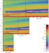 |
Fig. 1 Space-time diagram showing the evolution of the azimuthally-averaged gas surface density ∑, for the three runs ℳ300 (top panel), ℳ200 (middle panel), and ℳ10 (bottom panel). The radial extent of all the diagrams range from 0.08 rp,0 to 3rp,0, with the planet initially at rp,0 = 1. The fixed regime is separated from the migrating regime by the vertical black dashed line, and the instantaneous position of the planet is represented by the semi-transparent white line. The estimated inner and outer gap edges in the migrating regime are indicated by the black dotted lines. |
3.2 Planet migration and eccentricity
In order to better characterize how the planet migration is impacted by the planet gap shape, we plot in Fig. 2 the temporal evolution of the semi-major axis ap (left panel) and the eccentricity ep (right panel) of the planet for our three simulations.
The runs ℳ200 and ℳ300 exhibit a semi-major axis that slowly increases with time, which implies a slow outward migration on average. For a planet initially at 10 au, the migration rate would be on average ≃60 au Myr−1 for ℳ300 and ≃100 au Myr−1 for ℳ200 . In these two cases, the right panel of Fig. 2 shows two main phases for the eccentricity: a short phase of low eccentricity (<1%) for a few tens of orbits followed by an abrupt increase of the eccentricity (≃6–8%). In ℳ300 the eccentricity is globally increasing but quite variable, with an episode of lower eccentricity (≃1–2%) near 500 orbits corresponding to a migration stop in the left panel.
In ℳ10, the migration is activated as soon as the planet has reached its final mass at t = 10 orbits and before the planet has carved a gap. Fig. 2 confirms that the migration is divided in two regimes: a relatively fast inward migration at a rate ≃730 au Myr−1 for a planet initially at 10 au followed by a slow outward migration at a rate ≃60 au Myr−1 after an abrupt migration reversal at t = 50 orbits. In ℳ10, the planet orbit remains quasi-circular during the whole migration. We checked that the planet inclination is negligible compared to the planet eccentricity by at least two orders of magnitude.
We show a radial profile of the surface density ∑ in ℳ300 in Fig. 3, overlaid in purple with the locations of first-order external Lindblad resonances for m = 5 to m = 10. ∑ is here averaged azimuthally and temporally over 50 orbits for two epochs: when the planet migrates outward and is nearly circular at t ∈ [300– 350] orbits (ep ≲ 1.5%, black dashed line), and once the planet stalls and its eccentricity is close to 5% at t ∈ [400 – 4450] orbits (black solid line). At early times, we already detect a clear asymmetry of the gap shape that should participate in the torque imbalance and the outward planet migration, because outer principal resonances are expected to fall in the wide and deep outer gap, while inner principal resonances are expected to be enhanced by material accumulating close to the narrower and shallower inner gap.
By comparing the gap shape between both epochs, we first notice that there is a clear shift outwards of the solid line compared to the dashed line, at the location of the outer density maximum. This drift illustrates the progressive erosion of the outer disk by the gap and is due to the fast accretion driven by the wind in the gap (Martel & Lesur 2022, WFL23). As a result, mass progressively piles up in the inner gap, leading to the strong gap dissymmetry observed at later times. This negative density gradient locally around the planet is expected to negatively reinforce the corotation torque exerted onto the planet (Pepliński et al. 2008a,b), slowing down its migration.
Second, the gap is globally shallower at later times (solid line). This could be due to the increased planet eccentricity since one expects a shallower gap around a massive eccentric planet compared to a circular one (see Fig. 4 in Duffell & Chiang 2015).
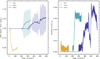 |
Fig. 2 Migration properties at different restart times and therefore for a different gap shape. Left: temporal evolution of the semi-major axis ap (solid lines) and radial position (shaded areas) of the planet. Whatever the initial condition, the planet migration is eventually slow and outward for β0 = 103 once the gap has been carved. Right: temporal evolution of the planet eccentricity ep, initially small (<1.5%) before increasing abruptly (≃7%) for the cases ℳ200 and ℳ300. |
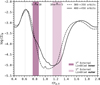 |
Fig. 3 Azimuthal average of the logarithm of the gas surface density ∑ for the run ℳ300 , temporally averaged during a phase of quasi-circular and outward migration (dashed line), and during a phase of stalled and eccentric migration (solid line). The two vertical gray dotted lines show the reconstructed radii where the main sources of high-frequency ΓLi variability are expected to originate from. The purple areas indicate the location of the inner and outer first-order external Lindblad resonances, for the modes m = 5 to m = 10. For the quasi-circular case (dashed line), the wind has already affected the planet gap, with a wider outer gap compared to the inner gap. For the eccentric case (solid line), the gap is globally denser due to the increase of the planet eccentricity. The wind has strongly enhanced the inner gap compared to the outer gap that is even further away from the planet location. The negative density gradient at the planet location could boost a negative corotation torque. |
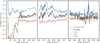 |
Fig. 4 Temporal evolution of various torque components exerted by the gas on the migrating planet and displayed with a moving average of 5 orbits, for the three runs ℳ10 (left panel), ℳ200 (middle panel), and ℳ300 (right panel). The total torque (black solid curves) is decomposed in three components, coming from different regions: the torque from the inner disk associated to the inner Lindblad torque 〈ΓLi 〉5orb (blue curves, 〈ΓLi 〉5orb ≳ 0), the torque from the outer disk associated to the outer Lindblad torque 〈ΓLo 〉5orb (red curves, 〈ΓLo 〉5orb ≲ 0), and the torque in the planet gap associated to the corotation torque 〈ΓC〉5orb (yellow curves, 〈ΓC〉5orb ≲ 0). All these torques are normalized by Γ0 . A proxy for the mass reservoir enclosed in the gap is represented via the black dashed line. |
3.3 Gravitational torques
In all cases, the planet eventually migrates outward once it has carved a deep gap, which seems quite robust for such a high value of the initial magnetization. In order to explain this migration behavior, we can study the gravitational torques1 of the gas onto the planet.
We plot in Fig. 4 the temporal evolution of the dimensionless gravitational torque 〈Γ〉5orb/Γ0 exerted by the disk onto the planet, with a moving average of 5 orbits and Γ0 =  , evaluated initially and at rp,0. We divided Γ in three components: the corotation torque ΓC in yellow, the inner Lindblad torque ΓLi in blue, and the outer Lindblad torque ΓLo in red. We defined the corotation region as the region where the fluid azimuthally-averaged horizontal velocity in the planet’s frame deviates significantly from a purely Keplerian flow. We chose the criterion |〈vr〉ϕ|/|〈vϕ〉ϕ| ≳ 4% in the midplane, smoothing the velocity fields radially and temporally over 1 orbit so as to capture almost the entire planet gap without being too sensitive to the local variability of the velocity fields. As mentioned in Section 3.1, the resulting estimate of the planet gap width is represented with the black lines in Fig. 1. We then computed the gravitational torque exerted by the gas inside the corotation region ⟨ΓC⟩5orb by summing the contribution of all the cells inside that region, excluding the effect of the gas inside the Hill sphere. Note that it is slightly different from what is computed in the simulations, as part of this material participates to the total torque, given a sin2(x) tapering function between 50% and 100% of the Hill sphere. The Lindblad torques are simply the sum of the contribution of the cells inside the planet gap’s inner edge (⟨ΓLi⟩5orb) and outside the planet gap’s outer edge (⟨ΓLo⟩5orb). The black dashed lines give an estimate of the gas mass included inside the corotation region, removing the contribution from the Hill sphere, and normalizing by a proxy of the mass reservoir initially available inside the gap. We therefore expect this quantity to decrease as a gap is carved by the planet, before reaching a quasi-constant value. Looking at the temporal evolution of these various gravitational torques, we see that the inner Lindblad torque is globally positive for all cases, whereas the corotation torque and the outer Lindblad torque tend to be negative.
In ℳ10 , the corotation torque and the outer Lindblad torque are strongly negative and dominate during the first 50 orbits, as a significant mass of gas material is contained inside the corotation region. Beyond 50 orbits, the corotation region has been depleted and reaches a few percents of the initial mass reservoir (see black dashed line), which decreases the amplitude of the corotation torque, whereas the inner Lindblad torque which slowly increases is eventually multiplied by two, and becomes the main driver of migration. This behavior of the torques confirms the migration pattern for this simulation, with a first phase of type-III-like inward migration with a partial gap, followed by a sudden migration stop when the dynamical corotation torque cancels out, and a migration reversal dominated by the behavior of the gas material inside the inner gap edge (see also Fig. 6 in Hu et al. 2025).
For ℳ200, |〈ΓLo〉5orb| is quite variable but globally decreases. This is probably because the outer gap erosion is faster than the outward planet migration rate, which decreases the contribution of the gas material outside the gap’s outer edge to 〈ΓLo〉5orb. For the same period of time, |〈ΓC〉5orb| is globally divided by two as the mass inside the gap is also divided by two. The main driver of migration is therefore ⟨ΓLi〉5orb > 0, with episodes of strong amplification of ⟨ΓLi〉5orb corresponding to phases of faster outward migration.
The behavior of the torques is roughly similar for the run ℳ300. The total torque is globally positive when t < 380 orbits, with a contribution of the torque components similar to that of ℳ200 . However, the behavior of the inner and corotation torques 〈ΓLi〉5orb and 〈ΓC〉5orb departs from what has been described earlier after t ≃ 380 orbits. In particular, there is a stronger variability inside the gap, associated with a doubling of both the mass inside the gap and |〈ΓC〉5orb|. We observe also that the gap’s inner edge slightly shrinks and gets closer to the planet location (black line in the top panel of Fig. 1), as the planet eccentricity exceeds ≃2%. The end result is that 〈ΓLi〉5orb is on average counterbalanced by 〈ΓC〉5orb, leading to a total torque that is nearly zero on average at t ≃ 400 orbits, and therefore a migration stall. In addition, the strong variability of 〈ΓLi〉5orb is sufficient to induce strong fluctuations in the semi-major axis and eccentricity of the planet (e.g., near t = 460 500 orbits).
This discussion highlights the correlation between the variability of 〈ΓLi〉 and the planet stochastic behavior. While a part of this variability might be associated with sporadic episodes of accretion through the gap driven by the wind torque, we find that 〈ΓLi〉 is also subject to rapid quasi-periodic oscillations at two characteristic frequencies: ω = ωp and ω ≃ 2ωp ≡ ωc (see Appendix A). While the first frequency can easily been understood as resulting from the planet’s eccentricity, the second one is more elusive. We can relate these frequencies to two corotation radii that we represent as two vertical gray dotted lines in Fig. 3. We find that ωc corresponds to the peak of the inner density ring lying at the gap edge around r ≃ 0.63rp,0 (see also top panel of Fig. 1). Density rings are known to be subject to the Rossby-Wave Instability (RWI, Lovelace et al. 1999), and we observe that an elongated vortex indeed develops at this location (see left panel of Fig. B.1). Therefore, we associate the quasi periodic oscillation at ωc of the inner Lindblad torque to a transient vortex triggered at the inner gap edge, lasting a few tens of orbits, but regenerated sporadically.
The corotation torque, and more specifically the gravitational torque measured in the gap region, is negative for two reasons. First, the contribution of the gas material accumulated near the outer wake and episodically carried inwards by the accretion flow accounts for a significant fraction of the total 〈ΓC〉5orb (see Appendix B for the shape of the horseshoe region). Second, the gap radial asymmetry leads to a negative density gradient at the planet location. This gradient is sharper at later times for the run ℳ300 (see solid line in Fig. 3), and could be responsible for the enhanced 〈ΓC〉5orb at t > 400 orbits in the right panel of Fig. 4.
3.4 Origin of the eccentricity
The aim of this section is to have a qualitative understanding of the processes behind the evolution of the planet eccentricity. To that end, we focus on the epoch of ep amplification for the run ℳ200 at t ∈ [206–248] orbits (see turquoise curve in the right panel of Fig. 2), and follow the semi-analytical work from Duffell & Chiang (2015). In particular, we make extensive use of their Appendix A and the formulae needed to evaluate the contributions to ėp from various resonances (Goldreich & Tremaine 1980; Papaloizou & Larwood 2000; Ogilvie & Lubow 2003). We focus on the principal Lindblad resonances (LR0), the first-order co-orbital (LR1c) and external (LR1e) Lindblad resonances, and the first-order corotation resonances (CR1). These resonances are called first-order resonances as the perturbing potential of an eccentric planet can be expanded as a principal component and a first-order component in the eccentricity (Masset 2008). Note that we do not write here the full set of equations required to compute ėp for all these resonances but refer the reader to the Appendix A of Duffell & Chiang (2015) for more details.
A general formula to derive the contribution of a first-order resonance ℛ to ėp can be written as a sum over azimuthal wave numbers m:
 (6)
(6)
where  is the planet’s angular momentum and depends on the planet properties (ap, ep, qp), mmax = (2h)−1 is a rough approximation of the torque cut-off for a nonself-gravitating disk (Goldreich & Tremaine 1980; Duffell & Chiang 2015). ℱw(ℛ) is a weakening function that may decrease the contribution to ėp of the m-fold component of the resonancedependent torque Tℛ (m), whether it be because of the increasingly supersonic motion of the epicyclic frequency for the Lindblad torques (Papaloizou & Larwood 2000; Fairbairn & Rafikov 2025) or a saturation function for the corotation torque (Ogilvie & Lubow 2003; Goldreich & Sari 2003).
The methodology that we chose here is semi-analytic as it relies on physical quantities estimated in ℳ200 at the location of the resonances, using the Keplerian frequency Ωp at the planet location. Thus, we measured on the one hand ∑ (r) at the location of the Lindblad resonances (LR0, LR1c, and LR1e), and on the other hand we needed ν(r), ∑ (r), and d∑ (r)/dr for CR1. For all these quantities, we systematically removed the contribution of the material inside the Hill sphere, as this region contains large and highly variable over-densities that analytic perturbative theories do not intend to treat. Because the turbulent viscosity in our simulations is not parametrized via an αν parameter (Shakura & Sunyaev 1973), we first measured for each snapshot in the simulation the radial Reynolds stress, and from this estimate we chose a constant ν = 1.25 × 10⁻⁶, corresponding to αν = 5 × 10⁻⁴ at r = rp,0. Our aim here is mainly to provide a simplified illustration of the behavior of the first-order corotation resonances, especially since we used a viscous formalism that is expected to be far from the real conditions of our simulations.
We plot in Fig. 5 the various contribution to the eccentricity evolution ėp/ep as a function of ep, for the run ℳ200 at t ∈ [206– 248] orbits. Because ep is roughly increasing with time during our epoch of interest, a higher ep in this graph indicates also a later period in the simulation. For a given planet eccentricity, ėp /ep < 0 means that the eccentricity will be damped and the planet will tend to be stabilized on a circular orbit. Conversely, ėp /ep > 0 means that the eccentricity will be excited and the planet will tend to be pushed into an even more eccentric orbit.
We first focus in Fig. 5 on the rainbow curve, which represents a smoothed numerical measure of ėp/ep as a function of ep , the colors indicating the temporal evolution from purple (t = 206 orbits) to red (t = 248 orbits). When ep ≲ 1% (purple to blue), ėp/ep alternates between negative and positive values, indicative of oscillations between phases of ep damping and ep driving. If ep somehow reaches higher values ep ∈ [1% – 7%] (green to orange), ėp/ep is always positive, and ep increases even more. Finally, when ep ≳ 7% (red), ėp/ep switches from positive to slightly negative values, meaning that ep reaches a plateau and slowly decreases. This picture is consistent with the right panel of Fig. 2 and is compatible with a finite-amplitude instability scenario (Goldreich & Sari 2003), which would be activated when  , and would be limited by the increasingly supersonic motion of the planet’s epicyclic frequency κp.
In order to test that scenario, we plot in Fig. 5 the contributions to the eccentricity evolution ėp/ep: LR0, CR1, LR1c, and LR1e as a function of ep . The sum of these contributions is represented by the red circles, to be compared qualitatively with the rainbow curve. We show with these red circles that ėp/ep is negative whenever ep << 2%, is positive and increasing when ep ≥ 2%, and eventually decreases when ep/h0 ≳ 1. The global evolution of ėp /ep is therefore consistent with a finite- amplitude instability: (i) ep is damped as long as the planet orbit is nearly circular. If the eccentricity reaches up to ≃1.5%, the planet is pushed back to a quasi-circular orbit. This behavior can be seen for all simulations in the right panel of Fig. 2, where the planet remains confined in the low-eccentricity regime and oscillates between 0 and 1.5% over a significant period of time (about 140, 20, and 75 orbits for ℳ10, ℳ200, and ℳ300 respectively). (ii) Beyond ep ≃ 2%, the eccentricity is amplified until ep ≃ h0, beyond which ėp/ep is still positive but the slope is negative, meaning that the eccentricity is less and less amplified. To understand this mechanism of saturation when ep/h0 ≃ 1, we define the velocity vϵ of the epicyclic motion as the product of half the epicyclic frequency κp (= Ωp for a Keplerian orbit) and the radial distance the planet crosses between its apastron radius rα = (1 + ep)ap and its periastron radius rπ = (1 − ep)ap:
 (7)
(7)
using the isothermal sound speed cs,0. vϵ is therefore supersonic when ep /h0 > 1, which may explain why the ep eventually stabilizes as it approaches 6–8% (Fairbairn & Rafikov 2025).
Looking at the contributions of the various resonances, we show that principal Lindblad resonances tend to damp the planet eccentricity (ėp(ℛ = LR0) < 0, consistent with an outward migration, see, e.g., Masset 2008, their Section. 5) but are negligible compared to first-order resonances, in agreement with Goldreich & Sari (2003); Duffell & Chiang (2015). First- order external Lindblad resonances LR1e are the only source of ep excitation and dominates the behavior of ėp when ep > 2%. They are counterbalanced at low ep << 2% by first-order co-orbital Lindblad (LR1c) and corotation resonances (CR0). However, these two damping mechanisms vanish as the gap density decreases (LR1c) and the saturation function ℱw(ℛ) decreases (CR0) when increasing ep . It is important to stress that our semi-analytic methodology relies on the estimate of ν, which strongly impacts ℱw(ℛ), and therefore determines precisely how fast the amplitude of ėp(ℛ = CR1)/ep < 0 goes to zero when increasing the eccentricity. Hence, our interpretation in only semi-quantitative.
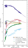 |
Fig. 5 Contribution of various resonances to the eccentricity evolution ėp / ep as a function of ep, for the run ℳ200 and during the episode of ep amplification at t ∈ [206–248] orbits. The semi-analytical decomposition focuses on the principal Lindblad resonances (LR0, yellow +), the first-order corotation resonances (CR1, green ×), the first-order coorbital (LR1c, light blue ◊), and external (LR1e, dark blue ★) Lindblad resonances. The sum of all these contributions are represented with red ◦. The rainbow curve represents a numerical measure of ėp/ep between t = 206 orbits (purple color) and t = 248 orbits (red color). Eccentricity growth is a finite-amplitude instability, with a damping of ep when ep < 1% or ep ≳ 7%, and an excitation of ep when ep ∈ [1.5% – 7%]. |
3.5 Eccentricity-driven accretion/ejection modulation
Now that we have a qualitative explanation of how the planet eccentricity is excited by the disk via first-order external Lindblad resonances, we seek to determine in this section the back- reaction of such a moderate eccentricity on the gaseous disk. To analyze the time-variability of the disk, we zoom on two epochs of 5 orbits in ℳ200: when the planet is quasi-circular at t = 206.4 orbits (epoch Γcirc), thus before the episode of ep amplification, and when the planet reaches a nearly maximum eccentricity at t = 244.85 orbits (epoch Γecc).
The 5-orbit evolution of the planet radius rp is shown in the top panel of Fig. 6 for both Γcirc (thick gray line) and Γecc (thin gray line). We also plot in the top panel of Fig. 6 the 5- orbit evolution of the accretion rate  through the gap. Each dot represents one snapshot of the simulation from which we reconstruct the accretion behavior in the planet gap. Interestingly, Ṁ varies weakly in the circular case (thick purple line), but exhibits a clear periodic modulation in the eccentric case (thin purple line), with a ratio between the maximum and minimum reaching 2.5. Because this modulation of Ṁ is not clearly detectable in the circular case and has a typical frequency close to κp in the eccentric case, we associate it to the planet eccentricity.
In the rest of this section, we focus on the eccentric case. In the bottom left panel of Fig. 6, we plot the space–time diagram of Ṁ. The eccentric orbit of the planet is represented by the white dots. We retrieve the eccentricity-driven modulation of the accretion, particularly visible in the outer gap and partly in the outer disk (r/rp,0 < 3). We notice also the propagation of sonic acoustic waves from the planet position towards the outer disk, due to the epicyclic motion of the planet. The characteristic of these acoustic waves are represented in the bottom left panel of Fig. 6 with green lozenges and match the perturb Ṁ accurately.
In the bottom right panel of Fig. 6, we plot the space-time diagram of the wind mass lass rate  , linked to the vertical mass flux and estimated at Θ+ = arctan(9h), well above the disk upper surface. ℰ+ is negative at θ = Θ+ if the flow locally falls back towards the disk midplane. We show that some material is periodically ejected vertically by the wind at Θ+ from ≃0.6 rp,0 to ≃2rp,0, and especially in the inner part of this wind region. The period of appearance of these ejecta is consistent with the epicyclic frequency of the eccentric planet. In order to apprehend the typical speed of propagation of these ejecta, we represent with blue lozenges the characteristic on an alfvén wave in the bottom right panel of Fig. 6. The relatively good match between the modulation of the wind ejection and the Alfvénic characteristic indicate that the planet eccentricity launches a modulation in the disk magnetosphere that travels along the magnetic field lines, possibly on long distances in the outflow.
We show in Fig. C.1 that the modulation of the wind mass loss rate is top-down asymmetric, with no modulation of ℰ− from the more massive wind estimated at θ = Θ = −Θ+, well below the disk’s lower surface. Due to the slight inclination of poloidal magnetic field lines at the disk surface, we expect the launching point of the modulated ejected material to originate from an upper accretion layer in the inner regions of the disk after an episode of strong Ṁ, but not from a lower accretion layer. This picture is indeed consistent with the fact that the accretion flows are also top-down asymmetric in the inner regions, with material crossing the inner gap and being elevated to a single accretion layer at the upper surface. Although this ℰ+ variability could be a physical process due to a significant fraction of accreted material being ejected from the inner disk after an episode of strong accretion, we cannot rule out the potential influence of the inner boundary conditions. Whatever the origin of its launching mechanism, the modulation of the mass loss rate is related to the forcing of the planet eccentricity.
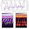 |
Fig. 6 Eccentricity-driven modulation of the accretion and ejection processes. Top: 5-orbit evolution of the planet radius rp (gray lines) and accretion rate in the planet gap 〈Ṁ〉gap (purple lines) during two epochs in the run ℳ200 : when the planet orbit is quasi-circular (thick lines) and once the planet eccentricity is nearly maximum (thin lines). Bottom: space-time diagram of the accretion rate Ṁ (left) and the ejection ℰ+ at arctan(9h) (right) during the 5-orbit evolution of the eccentric giant planet. The instantaneous radial position of the planet is shown with white circles. Some characteristic velocities indicate how planet-driven waves are propagating in the disk: the adiabatic sound speed cs in green and the Alfvén speed vA in blue. The gap location used to compute |

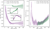 |
Fig. 7 Same as Fig. 2, but for a lower magnetization β0 = 105, and dividing the resolution by two in every direction. Migration is activated after 10 and 200 planet orbits for the violet and green curves respectively. Once a deep gap has been carved, migration is slow and ep slowly increases. |
3.6 Impact of the disk magnetization
The simulations presented above were all performed with a relatively strong large-scale field β = 103, and a natural question is to check the impact of weaker field on the planet’s dynamics. We therefore performed preliminary simulations with a lower magnetization (β0 = 105 ≡ β5) and a lower resolution (Nr/2 × Nθ/2 × Nϕ/2 = 256 × 128 × 512). We show in Fig. 7 the evolution of the semi-major axis (left panel) and the eccentricity (right panel) of the Jovian planet, activating the planet migration after the planet has reached its final mass at Trelease = 10 orbits (violet curve, run ℳ10(β5)) or waiting until a deep gap has been carved at Trelease = 200 orbits (green curve, run ℳ200(β5)). For ℳ10(β5) and before the gap is carved, the migration is fast and inwards for ≃200 orbits. The eccentricity increases for ≃40 orbits, before being quickly damped by first-order co-orbital resonances, probably due to the high density in the co-orbital region. Once the gap is formed (after 200 orbits), we find in both runs that there is almost no migration and the eccentricity slowly increases with a similar growth rate. We find as expected that the gap density is much lower when decreasing the magnetization (as already seen in simulations with fixed planets in WFL23), which suggests that first-order co-orbital resonances should not be able to damp the eccentricity. Moreover, Fig. 7 shows that ep still increases at β0 = 105, but with a much lower growth rate and a smaller variability compared to the case with β0 = 103 in Fig. 2. We suspect that accretion of matter continuously occurs in the gap with a slight gap asymmetry, enhancing first-order Lindblad resonances and therefore the eccentricity. In consequence, a stronger wind-driven accretion seems to favor eccentricity excitation via finite amplitude instability. The influence of the disk magnetization has yet to be confirmed via dedicated simulations, but their computational cost makes the exploration of parameter space prohibitive.
4 Summary and discussion
In this numerical study, we performed with the IDEFIX code three 3D non-ideal MHD simulations of a migrating Jovian planet in a wind-launching magnetized disk, focusing in particular on the impact of the planet gap shape. When t < Trelease, for an initial plasma parameter β0 = 103 and a constant aspect ratio h0 = 0.05, we retrieve the main results of WFL23 regarding a planet with qp = 10−3 on a fixed circular orbit in magnetized disks. In particular, the Jovian planet carves a radially asymmetric gap, which coexists with self-organized structures. Gas material crosses the gap via sporadic episodes of accretion and poloidal magnetic field is efficiently accumulated in this low density region, increasing locally the magnetic wind torque. Such enhanced magnetic wind in a planet-carved gap is compatible with the detection by Galloway-Sprietsma et al. (2023) of coherent upward flows arising from an annular gap in the AS 209 disk, near the location of a circumplanetary disk (CPD) candidate (Bae et al. 2022). Our main findings are:
In all cases, planet migration is slow and mainly outward once a deep gap has been carved. The corresponding migration speed is a few tens of au Myr−1 , for a planet initially in the 5–100 au range. Even if the planet’s semi-major axis increases on average, migration is still variable, with episodes of stalled migration and sometimes inward migration. Without a deep gap, the migration is initially faster and inwards until the amplitude of the corotation torque decreases abruptly, leading to a migration reversal and eventually a slow outward migration;
By delimiting the region enclosing the non-steady gap and examining the 5-orbit averaged gravitational torques, we show that the outer Lindblad torque 〈ΓLo〉5orb is negative with a decreasing amplitude with time, probably related to the typical timescale of the gap’s outward erosion being shorter than the typical timescale of the planet’s outward migration;
The inner Lindblad torque 〈ΓLi〉5orb is a source of outward migration, and both its global evolution and its variability have a strong influence on the total torque exerted on the Jovian planet, and therefore on its direction and amplitude of migration. The spikes of the instantaneous ΓLi are partly due to an episodically denser inner ring leading to sporadic vortex formation through RWI at this location;
The torque in the corotation region 〈ΓC〉5orb is always negative due to (i) the over-density of material captured in the outer planet wake that tends to be carried inwards by the accretion flow; (ii) the negative density gradient at the planet location due to the gap’s radial asymmetry. At later times , this density gradient could enhance negatively 〈ΓC〉5orb and counterbalance the mean positive value of 〈ΓLi〉5orb, leading to episodes of stalled migration;
In most cases, the planet is found to be eccentric, with two main phases: ep is low (≲1.5%) initially, and eventually increases to moderate values (≃7%). Such eccentricity evolution is consistent with a finite-amplitude instability: (i) first-order corotation resonances damp any wind-driven eccentricity perturbation to a circular orbit (ep ≪ 1%), but saturate quickly at slightly higher eccentricities; (ii) first-order coorbital Lindblad resonances take over and stabilize small eccentricities (ep ≲ 1.5%), possibly due to the increase in the gap’s surface density with eccentricity; (iii) first-order external Lindblad resonances dominate and quickly excite moderate eccentricities (ep ≳ 2%), but are limited by the increasingly supersonic planet’s epicyclic motion when ep ≃ 6–8%;
The accretion rate in the gap is modulated by the planet eccentricity, with alternating phases of low and higher accretion, as well as sonic waves propagating from the planet towards the outer disk. The wind mass loss rate at high altitudes also appears to be modulated by the planet eccentricity, and could originate from the upper accretion layer crossing the disk’s inner region, just inside the gap’s inner edge.
These results depart from the classical turbulent disk models. It is therefore necessary to build a new planet migration theory dedicated to the wind-driven accretion paradigm, as the notions developed in the classical viscous migration theory do not apply straightforwardly. An important next step for this 3D non-ideal MHD study would be to develop a simple framework for wind-driven accretion in 2D planet-disk simulations. In such a model, both the wind torque and mass loss rate would depend on the magnetic field strength and, consequently, on the distribution of magnetic flux, as proposed in Lesur (2021). However, gaps – whether formed by planets or self-organization – efficiently accumulate magnetic flux. Therefore, a predictive theory must account for magnetic flux transport and its accumulation in gaps. Currently, no such theory exists, leaving 2D simulations without a proper “effective” model.
4.1 Vortex-driven migration with laminar accretion flows
Lega et al. (2021, 2022) obtained a two-phased migration of Jovian planets in 3D low-viscosity disks with prescribed wind-driven angular momentum removal. In the first phase, a vortex develops at the gap’s outer edge, driving an inward migration, and eventually disappears. In the second phase, inward migration accelerates as accretion is increasingly blocked by the planet, with the fastest migration occurring when gas material piles up at the gap’s outer edge, and slower migration when accretion is unaffected by the planet gap. Our results are similar regarding the underlying mechanisms at play, with both an effect of a vortex and the accretion behavior, but reversed. Wind-driven accretion is actually not blocked by the gap, and is on average slightly decreased (increased) at the inner (outer) edge of the gap, leading to a gas pile-up (depletion) at that location. Such gas depletion impedes any inward migration, whereas the inner gas pile-up drives an outward migration. As the inner ring is enhanced by sporadic episodes of accretion, it eventually becomes unstable to the RWI, episodically forming a decaying vortex for a few tens of orbits.
4.2 Long-term evolution
We have seen through the paper that the radial asymmetry of the planet gap at high magnetization has a strong influence on the planet’s orbital properties. However, the longest migration phase presented here lasted 300 orbits, which corresponds to Tmigration ≃ 10 kyr for a planet initially at 10 au. Such value is a few hundred times smaller than the typical lifetime of a circumstellar disk, and raises the question of the long-term evolution of planet–disk–wind interactions. In particular, the radial drift of the outer gap edge has a typical velocity of ≃160 au Myr−1 for ℳ300 and ≃260 au Myr−1 for ℳ200, which is typically ≃2.5 times faster than the typical migration rate of the planet in both cases (see Section 3.2). Depending on observational constraints and to limit this efficient expansion effect, a lower magnetization could decrease the typical speed of the gap drift. For β0 = 103 and if the gap expansion remains the same after a few million years, we could end up with a single planet that has created a wide cavity of its own. Results from viscous simulations of disk-planet interactions in large inner cavities show that the eccentricity of massive planets is strongly increased (≃0.4) by first-order external Lindblad resonances (see, e.g., Papaloizou et al. 2001; Debras et al. 2021, and Section 3.4). We might therefore expect a similar eccentricity amplification for long-term planet-disk-wind simulations, but with an eccentric outward migration rather than an inward migration, and with observational signatures similar to those studied in Baruteau et al. (2021).
4.3 Eccentric planets and structured winds
de Valon et al. (2022) observed discrete structures (arches, cusps, fingers) in the rotating conical CO outflow of the DG Tau B system. They argue that the morphology and kinematics of this structured outflow is consistent with a steady MHD disk wind perturbed by quasi periodic brightness enhancements. They also show that the typical timescale between these enhancements is Tχ ∈ [190–490] years (see the right panel of Fig. 14 in de Valon et al. 2020). Assuming that this typical period is linked to the epicyclic frequency κp = 2π/Tχ of an eccentric giant planet modulating in a periodic way the ejection rate, we can simply use Kepler’s third law to retrieve the putative location aχ of the eccentric perturber in the disk, which gives aχ ∈ [33–62] au for DG Tau B. We note that de Valon et al. (2020) detected a dark ring in the radio emission of DG Tau B at rdip ≃ 53 ± 5 au, which falls inside our numerical estimate. Note that in order to establish a direct connection between the eccentricity-driven modulation of the mass loss rate and the wind structures in DG Tau B, we need to perform more detailed and precise computations, in particular via radiative transfer calculations that are beyond the scope of this paper. Nonetheless, an extension to this work would be to evaluate the visibility and detectability of the ejecta we observe in our simulations, but also to analyze how they propagate on vertical scales much larger than those considered here.
Acknowledgements
The authors acknowledge support from the European Research Council (ERC) under the European Union Horizon 2020 research and innovation program (Grant agreement No. 815559 (MHDiscs)). This work was granted access to the HPC resources of IDRIS under the allocations A0140402231 and A0160402231 made by GENCI. The 3D simulations were performed with the versions v1.1 and 2.0.04 of IDEFIX. Some of the computations presented in this paper were performed using the GRICAD infrastructure, which is supported by Grenoble research communities. The data presented in this work were processed and plotted with Python via various libraries, in particular numpy, matplotlib, scipy, and cmasher, but also the following personal projects under development: nonos to analyze results from IDEFIX simulations, cblind for most of the colormaps and lick for the visualizations in line integral convolution. IA tools have occasionally been used for debugging and reformulation. G.W.F. wishes to thank Clément Baruteau for fruitful scientific discussions, and Clément Robert for useful insights on code maintenance and development.
Appendix A High-frequency variability of the inner Lindblad torque
In the top panels of Fig. A.1, we present the temporal evolution of the instantaneous inner Lindblad torque ΓLi normalized by Γ0 , for three epochs in the run ℳ200. Using a Fourier analysis, we obtain in the bottom panels of Fig. A.1 the power spectra of ΓLi for the three epochs of interest. Depending on the epoch, we show that the two typical frequencies ωp ≃ 1 and ωc ≃ 2 that appear in the power spectra are consistent with an eccentric forcing of the planet and a strong m = 1 vortex sporadically developing at the location of the inner density ring:
For t ∈ [200 – 210] orbits (left panels of Fig. A.1), the planet is in a quasi-circular orbit and ωp is not clearly visible. On the contrary, ωc is dominant while the 5-orbit averaged ⟨ΓLi ⟩5orb is peaking in the middle panel of Fig. 4.
For t ∈ [220 – 240] orbits (middle panels of Fig. A.1), ωp and ωc are both present in the power spectrum, while both the planet eccentricity and ⟨ΓLi ⟩5orb strongly increase.
For t ∈ [300 – 325] orbits (right panels of Fig. A.1), the planet is eccentric while ⟨ΓLi⟩5orb is small and constant. During this epoch, the power spectrum of ΓLi indicates indeed that ωp is the dominant source of high-frequency variability.
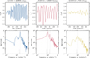 |
Fig. A.1 10-orbit temporal evolution (top panels) and power-spectrum (bottom panels) of the instantaneous inner Lindblad torque ΓLi, for three epochs in the run ℳ200 . Left panels: the planet is in a quasi-circular orbit and the 5-orbit averaged torque ⟨ΓLi⟩5orb is peaking in Fig. 4. Middle panels: the planet orbit becomes eccentric and ⟨ΓLi⟩5orb is peaking. Right panels: the planet orbit is eccentric and ⟨ΓLi⟩5orb does not vary. Depending on the epoch, we retrieve two typical frequencies ωp ≃ 1 and ωc ≃ 2 (vertical dotted lines). |
Appendix B Flow in the horseshoe region
We plot in the left panel Fig. B.1 the structure of the flow around the planet for the run ℳ300 at t = 490.75 orbits, in a cartesian plane (x/xp,0,y/yp,0) with 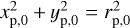 . The planet carves a deep annular gap, and we focus on this region in the right panel of Fig. B.1. We note the presence of the strong elongated vortex near the gap’s inner edge, which is a source of variability of 〈ΓLi〉5orb. Not only is the gap radially asymmetric, it is also azimuthally asymmetric. Let us define the azimuth of the planet ϕp. The horseshoe region on the trailing side (ϕ < ϕp) of the planet is reduced and is on average subject to a mass excess, unlike the region on the leading side (ϕ > ϕp) of the planet which is subject on average to a mass deficit. This imbalance may be responsible for a fraction of the negative corotation torque. This gas dynamics we observe in the gap region is in fact the opposite of the prediction by Kimmig et al. (2020), and can be interpreted the following way. Because the horseshoe orbits are disrupted by the accretion flow, some material is able to perform horseshoe U-turns on the trailing side close to the planet, but along the U-turn the material is progressively pushed inwards by the accretion flow until it reaches the inner gap edge, no further than an azimuth ϕ ≈ ϕp − π/2 on average, and therefore well before reaching the leading side close to the planet at ϕp – 2π. This strong azimuthal asymmetry of the horseshoe region makes the corotation torque unsaturated and negative due to the accumulation of material close to the trailing side of the planet, always replenished by the radial accretion flow . In particular, the over-density of material captured in the outer planet wake tends to be carried away by the accretion flow (see over-dense material at (r, ϕ) ≈ (1.15 rp,0, ϕp − π/2)), crossing the gap beneath the planet in azimuth and reaching the inner gap edge afterwards.
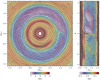 |
Fig. B.1 Gas flows around the planet for the run ℳ300 at t = 490.75 orbits. The background color represents the logarithm of the gas surface density. The black streamlines and the LIC (Line Integral Convolution) correspond to the radial and azimuthal components of the horizontal velocity, in the midplane and in the planet’s reference frame. The white lines indicate the estimated inner and outer gap edge. The right panel focuses on the horseshoe region. |
Appendix C Eccentricity-driven ejection modulation at two opposite surfaces
In Fig. C.1, we plot the temporal evolution over 5 orbits of the wind mass loss rate ℰ+ and ℰ− at two opposite latitudes far from the disk surfaces, respectively at Θ+ = arctan(9h) ≫ θ+ = arctan(3h) and Θ− = −Θ+. The top panel of Fig. C.1 shows ℰ+ (thin red line) and ℰ− (thick red line) integrated on the radial interval [0.6rp,0 − 0.8rp,0], thus coming from the inner disk region. The bottom panels of Fig. C.1 show the spacetime diagrams for ℰ+ (left) and ℰ− (right), obtained by performing a radial average over a moving radial band with a width of 0.2rp,0. We retrieve an eccentricity-driven modulation of ℰ+ which seems to originate from an upper accretion layer also modulated by the planet eccentricity. In contrast, the profile of ℰ− remains relatively flat over time.
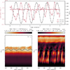 |
Fig. C.1 Eccentricity-driven modulation of the ejection processes at two surfaces θ = Θ+ = arctan(9h) and θ = Θ− = − arctan(9h) for the run ℳ200. Top panel: 5-orbit evolution of the planet radius rp (gray line) and of the wind mass loss rate, averaged over the radial interval [0.6rp,0 − 0.8rp,0], and estimated at Θ+ (thin red line) and Θ− (thick red line). Bottom panels: 5-orbit space-time diagrams of ℰ− (left panel) and ℰ+ (right panel). The instantaneous radial position of the planet is indicated with white circles, and the radial interval used to average ℰ in the top panel is indicated by white dashed rectangles. |
References
- Andrews, S. M., Huang, J., Pérez, L. M., et al. 2018, ApJ, 869, L41 [NASA ADS] [CrossRef] [Google Scholar]
- Aoyama, Y., & Bai, X.-N. 2023, ApJ, 946, 5 [NASA ADS] [CrossRef] [Google Scholar]
- Bai, X.-N., & Stone, J. M. 2013, ApJ, 769, 76 [Google Scholar]
- Bae, J., Teague, R., Andrews, S. M., et al. 2022, ApJ, 934, L20 [NASA ADS] [CrossRef] [Google Scholar]
- Balbus, S. A., & Hawley, J. F. 1991, ApJ, 376, 214 [Google Scholar]
- Baruteau, C., Wafflard-Fernandez, G., Le Gal, R., et al. 2021, MNRAS, 505, 359 [NASA ADS] [CrossRef] [Google Scholar]
- Béthune, W., Lesur, G., & Ferreira, J. 2017, A&A, 600, A75 [NASA ADS] [CrossRef] [EDP Sciences] [Google Scholar]
- Bitsch, B., Crida, A., Libert, A. S., & Lega, E. 2013, A&A, 555, A124 [NASA ADS] [CrossRef] [EDP Sciences] [Google Scholar]
- Blandford, R. D., & Payne, D. G. 1982, MNRAS, 199, 883 [CrossRef] [Google Scholar]
- Chatterjee, S., Ford, E. B., Matsumura, S., & Rasio, F. A. 2008, ApJ, 686, 580 [NASA ADS] [CrossRef] [Google Scholar]
- Crida, A., Baruteau, C., Kley, W., & Masset, F. 2009, A&A, 502, 679 [NASA ADS] [CrossRef] [EDP Sciences] [Google Scholar]
- Cui, C., & Bai, X.-N. 2021, MNRAS, 507, 1106 [NASA ADS] [CrossRef] [Google Scholar]
- Dawson, R. I., & Johnson, J. A. 2018, ARA&A, 56, 175 [Google Scholar]
- de Valon, A., Dougados, C., Cabrit, S., et al. 2020, A&A, 634, L12 [NASA ADS] [CrossRef] [EDP Sciences] [Google Scholar]
- de Valon, A., Dougados, C., Cabrit, S., et al. 2022, A&A, 668, A78 [NASA ADS] [CrossRef] [EDP Sciences] [Google Scholar]
- Debras, F., Baruteau, C., & Donati, J.-F. 2021, MNRAS, 500, 1621 [Google Scholar]
- Drążkowska, J., Bitsch, B., Lambrechts, M., et al. 2023, in Astronomical Society of the Pacific Conference Series, 534, Protostars and Planets VII, eds. S. Inutsuka, Y. Aikawa, T. Muto, K. Tomida, & M. Tamura, 717 [Google Scholar]
- Duffell, P. C., & Chiang, E. 2015, ApJ, 812, 94 [NASA ADS] [CrossRef] [Google Scholar]
- Duffell, P. C., Haiman, Z., MacFadyen, A. I., D’Orazio, D. J., & Farris, B. D. 2014, ApJ, 792, L10 [Google Scholar]
- Fairbairn, C. W., & Rafikov, R. R. 2025, MNRAS, 537, 1779 [NASA ADS] [Google Scholar]
- Galloway-Sprietsma, M., Bae, J., Teague, R., et al. 2023, ApJ, 950, 147 [NASA ADS] [CrossRef] [Google Scholar]
- Goldreich, P., & Tremaine, S. 1980, ApJ, 241, 425 [Google Scholar]
- Goldreich, P., & Sari, R. 2003, ApJ, 585, 1024 [Google Scholar]
- Hu, X., Li, Z.-Y., Wang, L., Zhu, Z., & Bae, J. 2023, MNRAS, 523, 4883 [NASA ADS] [CrossRef] [Google Scholar]
- Hu, X., Li, Z.-Y., Bae, J., & Zhu, Z. 2025, MNRAS, 536, 1374 [NASA ADS] [Google Scholar]
- Kimmig, C. N., Dullemond, C. P., & Kley, W. 2020, A&A, 633, A4 [NASA ADS] [CrossRef] [EDP Sciences] [Google Scholar]
- Lega, E., Nelson, R. P., Morbidelli, A., et al. 2021, A&A, 646, A166 [NASA ADS] [CrossRef] [EDP Sciences] [Google Scholar]
- Lega, E., Morbidelli, A., Nelson, R. P., et al. 2022, A&A, 658, A32 [NASA ADS] [CrossRef] [EDP Sciences] [Google Scholar]
- Lesur, G. R. J. 2021, A&A, 650, A35 [NASA ADS] [CrossRef] [EDP Sciences] [Google Scholar]
- Lesur, G., Kunz, M. W., & Fromang, S. 2014, A&A, 566, A56 [NASA ADS] [CrossRef] [EDP Sciences] [Google Scholar]
- Lesur, G., Flock, M., Ercolano, B., et al. 2023a, in Astronomical Society of the Pacific Conference Series, 534, Protostars and Planets VII, eds. S. Inutsuka, Y. Aikawa, T. Muto, K. Tomida, & M. Tamura, 465 [Google Scholar]
- Lesur, G. R. J., Baghdadi, S., Wafflard-Fernandez, G., et al. 2023b, A&A, 677, A9 [NASA ADS] [CrossRef] [EDP Sciences] [Google Scholar]
- Lin, D. N. C., & Papaloizou, J. 1986a, ApJ, 307, 395 [Google Scholar]
- Lin, D. N. C., & Papaloizou, J. 1986b, ApJ, 309, 846 [Google Scholar]
- Louvet, F., Dougados, C., Cabrit, S., et al. 2018, A&A, 618, A120 [NASA ADS] [CrossRef] [EDP Sciences] [Google Scholar]
- Lovelace, R. V. E., Li, H., Colgate, S. A., & Nelson, A. F. 1999, ApJ, 513, 805 [NASA ADS] [CrossRef] [Google Scholar]
- Manger, N., Pfeil, T., & Klahr, H. 2021, MNRAS, 508, 5402 [NASA ADS] [CrossRef] [Google Scholar]
- Martel, É., & Lesur, G. 2022, A&A, 667, A17 [NASA ADS] [CrossRef] [EDP Sciences] [Google Scholar]
- Masset, F. 2000, A&AS, 141, 165 [NASA ADS] [CrossRef] [EDP Sciences] [Google Scholar]
- Masset, F. S. 2008, in EAS Publications Series, 29, eds. M. J. Goupil & J. P. Zahn, 165 [NASA ADS] [CrossRef] [EDP Sciences] [Google Scholar]
- Masset, F. S., & Papaloizou, J. C. B. 2003, ApJ, 588, 494 [NASA ADS] [CrossRef] [Google Scholar]
- Mauxion, J., Lesur, G., & Maret, S. 2024, A&A, 686, A253 [NASA ADS] [CrossRef] [EDP Sciences] [Google Scholar]
- Nelson, R. P., Gressel, O., & Umurhan, O. M. 2013, MNRAS, 435, 2610 [Google Scholar]
- Ogilvie, G. I., & Lubow, S. H. 2003, ApJ, 587, 398 [NASA ADS] [CrossRef] [Google Scholar]
- Paardekooper, S., Dong, R., Duffell, P., et al. 2023, in Astronomical Society of the Pacific Conference Series, 534, Protostars and Planets VII, eds. S. Inutsuka, Y. Aikawa, T. Muto, K. Tomida, & M. Tamura, 685 [Google Scholar]
- Papaloizou, J. C. B., & Larwood, J. D. 2000, MNRAS, 315, 823 [Google Scholar]
- Papaloizou, J. C. B., Nelson, R. P., & Masset, F. 2001, A&A, 366, 263 [NASA ADS] [CrossRef] [EDP Sciences] [Google Scholar]
- Pascucci, I., Cabrit, S., Edwards, S., et al. 2023, in Astronomical Society of the Pacific Conference Series, 534, Protostars and Planets VII, eds. S. Inutsuka, Y. Aikawa, T. Muto, K. Tomida, & M. Tamura, 567 [Google Scholar]
- Pepliński, A., Artymowicz, P., & Mellema, G. 2008a, MNRAS, 386, 164 [CrossRef] [Google Scholar]
- Pepliński, A., Artymowicz, P., & Mellema, G. 2008b, MNRAS, 386, 179 [CrossRef] [Google Scholar]
- Pepliński, A., Artymowicz, P., & Mellema, G. 2008c, MNRAS, 387, 1063 [CrossRef] [Google Scholar]
- Perez-Becker, D., & Chiang, E. 2011a, ApJ, 735, 8 [Google Scholar]
- Perez-Becker, D., & Chiang, E. 2011b, ApJ, 727, 2 [Google Scholar]
- Pinte, C., Dent, W. R. F., Ménard, F., et al. 2016, ApJ, 816, 25 [Google Scholar]
- Riols, A., Lesur, G., & Menard, F. 2020, A&A, 639, A95 [NASA ADS] [CrossRef] [EDP Sciences] [Google Scholar]
- Robert, C. M. T., Crida, A., Lega, E., Méheut, H., & Morbidelli, A. 2018, A&A, 617, A98 [NASA ADS] [CrossRef] [EDP Sciences] [Google Scholar]
- Shakura, N. I., & Sunyaev, R. A. 1973, A&A, 24, 337 [NASA ADS] [Google Scholar]
- Stoll, M. H. R., & Kley, W. 2014, A&A, 572, A77 [NASA ADS] [CrossRef] [EDP Sciences] [Google Scholar]
- Suriano, S. S., Li, Z.-Y., Krasnopolsky, R., & Shang, H. 2017, MNRAS, 468, 3850 [NASA ADS] [CrossRef] [Google Scholar]
- Suriano, S. S., Li, Z.-Y., Krasnopolsky, R., & Shang, H. 2018, MNRAS, 477, 1239 [NASA ADS] [CrossRef] [Google Scholar]
- Suriano, S. S., Li, Z.-Y., Krasnopolsky, R., Suzuki, T. K., & Shang, H. 2019, MNRAS, 484, 107 [NASA ADS] [CrossRef] [Google Scholar]
- Thi, W. F., Lesur, G., Woitke, P., et al. 2019, A&A, 632, A44 [NASA ADS] [CrossRef] [EDP Sciences] [Google Scholar]
- Van den Bossche, M., Lesur, G., & Dubus, G. 2023, A&A, 677, A10 [NASA ADS] [CrossRef] [EDP Sciences] [Google Scholar]
- Venuti, L., Bouvier, J., Flaccomio, E., et al. 2014, A&A, 570, A82 [NASA ADS] [CrossRef] [EDP Sciences] [Google Scholar]
- Villenave, M., Ménard, F., Dent, W. R. F., et al. 2020, A&A, 642, A164 [EDP Sciences] [Google Scholar]
- Wafflard-Fernandez, G., & Lesur, G. 2023, A&A, 677, A70 [NASA ADS] [CrossRef] [EDP Sciences] [Google Scholar]
- Wardle, M., & Koenigl, A. 1993, ApJ, 410, 218 [Google Scholar]
- Wu, Y., & Chen, Y.-X. 2025, MNRAS, 536, L13 [Google Scholar]
- Zhang, B., Sorathia, K. A., Lyon, J. G., Merkin, V. G., & Wiltberger, M. 2019, J. Computat. Phys., 376, 276 [NASA ADS] [CrossRef] [Google Scholar]
- Zhu, Z., & Stone, J. M. 2018, ApJ, 857, 34 [Google Scholar]
In general we cannot interpret the direction and amplitude of migration of an eccentric planet directly from the temporal evolution of the gravitational torque only, and we need to rather rely on the gravitational power. We checked here that the sign and qualitative behavior of the power and the torque are close to one each other, except for a slightly stronger variability for the power.
All Figures
|
Fig. 1 Space-time diagram showing the evolution of the azimuthally-averaged gas surface density ∑, for the three runs ℳ300 (top panel), ℳ200 (middle panel), and ℳ10 (bottom panel). The radial extent of all the diagrams range from 0.08 rp,0 to 3rp,0, with the planet initially at rp,0 = 1. The fixed regime is separated from the migrating regime by the vertical black dashed line, and the instantaneous position of the planet is represented by the semi-transparent white line. The estimated inner and outer gap edges in the migrating regime are indicated by the black dotted lines. |
| In the text | |
|
Fig. 2 Migration properties at different restart times and therefore for a different gap shape. Left: temporal evolution of the semi-major axis ap (solid lines) and radial position (shaded areas) of the planet. Whatever the initial condition, the planet migration is eventually slow and outward for β0 = 103 once the gap has been carved. Right: temporal evolution of the planet eccentricity ep, initially small (<1.5%) before increasing abruptly (≃7%) for the cases ℳ200 and ℳ300. |
| In the text | |
|
Fig. 3 Azimuthal average of the logarithm of the gas surface density ∑ for the run ℳ300 , temporally averaged during a phase of quasi-circular and outward migration (dashed line), and during a phase of stalled and eccentric migration (solid line). The two vertical gray dotted lines show the reconstructed radii where the main sources of high-frequency ΓLi variability are expected to originate from. The purple areas indicate the location of the inner and outer first-order external Lindblad resonances, for the modes m = 5 to m = 10. For the quasi-circular case (dashed line), the wind has already affected the planet gap, with a wider outer gap compared to the inner gap. For the eccentric case (solid line), the gap is globally denser due to the increase of the planet eccentricity. The wind has strongly enhanced the inner gap compared to the outer gap that is even further away from the planet location. The negative density gradient at the planet location could boost a negative corotation torque. |
| In the text | |
|
Fig. 4 Temporal evolution of various torque components exerted by the gas on the migrating planet and displayed with a moving average of 5 orbits, for the three runs ℳ10 (left panel), ℳ200 (middle panel), and ℳ300 (right panel). The total torque (black solid curves) is decomposed in three components, coming from different regions: the torque from the inner disk associated to the inner Lindblad torque 〈ΓLi 〉5orb (blue curves, 〈ΓLi 〉5orb ≳ 0), the torque from the outer disk associated to the outer Lindblad torque 〈ΓLo 〉5orb (red curves, 〈ΓLo 〉5orb ≲ 0), and the torque in the planet gap associated to the corotation torque 〈ΓC〉5orb (yellow curves, 〈ΓC〉5orb ≲ 0). All these torques are normalized by Γ0 . A proxy for the mass reservoir enclosed in the gap is represented via the black dashed line. |
| In the text | |
|
Fig. 5 Contribution of various resonances to the eccentricity evolution ėp / ep as a function of ep, for the run ℳ200 and during the episode of ep amplification at t ∈ [206–248] orbits. The semi-analytical decomposition focuses on the principal Lindblad resonances (LR0, yellow +), the first-order corotation resonances (CR1, green ×), the first-order coorbital (LR1c, light blue ◊), and external (LR1e, dark blue ★) Lindblad resonances. The sum of all these contributions are represented with red ◦. The rainbow curve represents a numerical measure of ėp/ep between t = 206 orbits (purple color) and t = 248 orbits (red color). Eccentricity growth is a finite-amplitude instability, with a damping of ep when ep < 1% or ep ≳ 7%, and an excitation of ep when ep ∈ [1.5% – 7%]. |
| In the text | |
|
Fig. 6 Eccentricity-driven modulation of the accretion and ejection processes. Top: 5-orbit evolution of the planet radius rp (gray lines) and accretion rate in the planet gap 〈Ṁ〉gap (purple lines) during two epochs in the run ℳ200 : when the planet orbit is quasi-circular (thick lines) and once the planet eccentricity is nearly maximum (thin lines). Bottom: space-time diagram of the accretion rate Ṁ (left) and the ejection ℰ+ at arctan(9h) (right) during the 5-orbit evolution of the eccentric giant planet. The instantaneous radial position of the planet is shown with white circles. Some characteristic velocities indicate how planet-driven waves are propagating in the disk: the adiabatic sound speed cs in green and the Alfvén speed vA in blue. The gap location used to compute |
| In the text | |
|
Fig. 7 Same as Fig. 2, but for a lower magnetization β0 = 105, and dividing the resolution by two in every direction. Migration is activated after 10 and 200 planet orbits for the violet and green curves respectively. Once a deep gap has been carved, migration is slow and ep slowly increases. |
| In the text | |
|
Fig. A.1 10-orbit temporal evolution (top panels) and power-spectrum (bottom panels) of the instantaneous inner Lindblad torque ΓLi, for three epochs in the run ℳ200 . Left panels: the planet is in a quasi-circular orbit and the 5-orbit averaged torque ⟨ΓLi⟩5orb is peaking in Fig. 4. Middle panels: the planet orbit becomes eccentric and ⟨ΓLi⟩5orb is peaking. Right panels: the planet orbit is eccentric and ⟨ΓLi⟩5orb does not vary. Depending on the epoch, we retrieve two typical frequencies ωp ≃ 1 and ωc ≃ 2 (vertical dotted lines). |
| In the text | |
|
Fig. B.1 Gas flows around the planet for the run ℳ300 at t = 490.75 orbits. The background color represents the logarithm of the gas surface density. The black streamlines and the LIC (Line Integral Convolution) correspond to the radial and azimuthal components of the horizontal velocity, in the midplane and in the planet’s reference frame. The white lines indicate the estimated inner and outer gap edge. The right panel focuses on the horseshoe region. |
| In the text | |
|
Fig. C.1 Eccentricity-driven modulation of the ejection processes at two surfaces θ = Θ+ = arctan(9h) and θ = Θ− = − arctan(9h) for the run ℳ200. Top panel: 5-orbit evolution of the planet radius rp (gray line) and of the wind mass loss rate, averaged over the radial interval [0.6rp,0 − 0.8rp,0], and estimated at Θ+ (thin red line) and Θ− (thick red line). Bottom panels: 5-orbit space-time diagrams of ℰ− (left panel) and ℰ+ (right panel). The instantaneous radial position of the planet is indicated with white circles, and the radial interval used to average ℰ in the top panel is indicated by white dashed rectangles. |
| In the text | |
Current usage metrics show cumulative count of Article Views (full-text article views including HTML views, PDF and ePub downloads, according to the available data) and Abstracts Views on Vision4Press platform.
Data correspond to usage on the plateform after 2015. The current usage metrics is available 48-96 hours after online publication and is updated daily on week days.
Initial download of the metrics may take a while.